Chapter 16 Understanding Relationships Numerical Data … · Chapter 16 Understanding ... Numerical Data Part 2 Section 16.1 Exercise Set 1 16.1: (a) deterministic (b) ... ©2014

1

©2014 Cengage Learning. All Rights Reserved. May not be scanned, copied, or duplicated, or posted to a publicly accessible website, in whole or in part.

AP* SOLUTIONS

Chapter 16 Understanding Relationships – Numerical Data Part 2

Section 16.1 Exercise Set 1

16.1: (a) deterministic

(b) probabilistic

(c) probabilistic

(d) deterministic

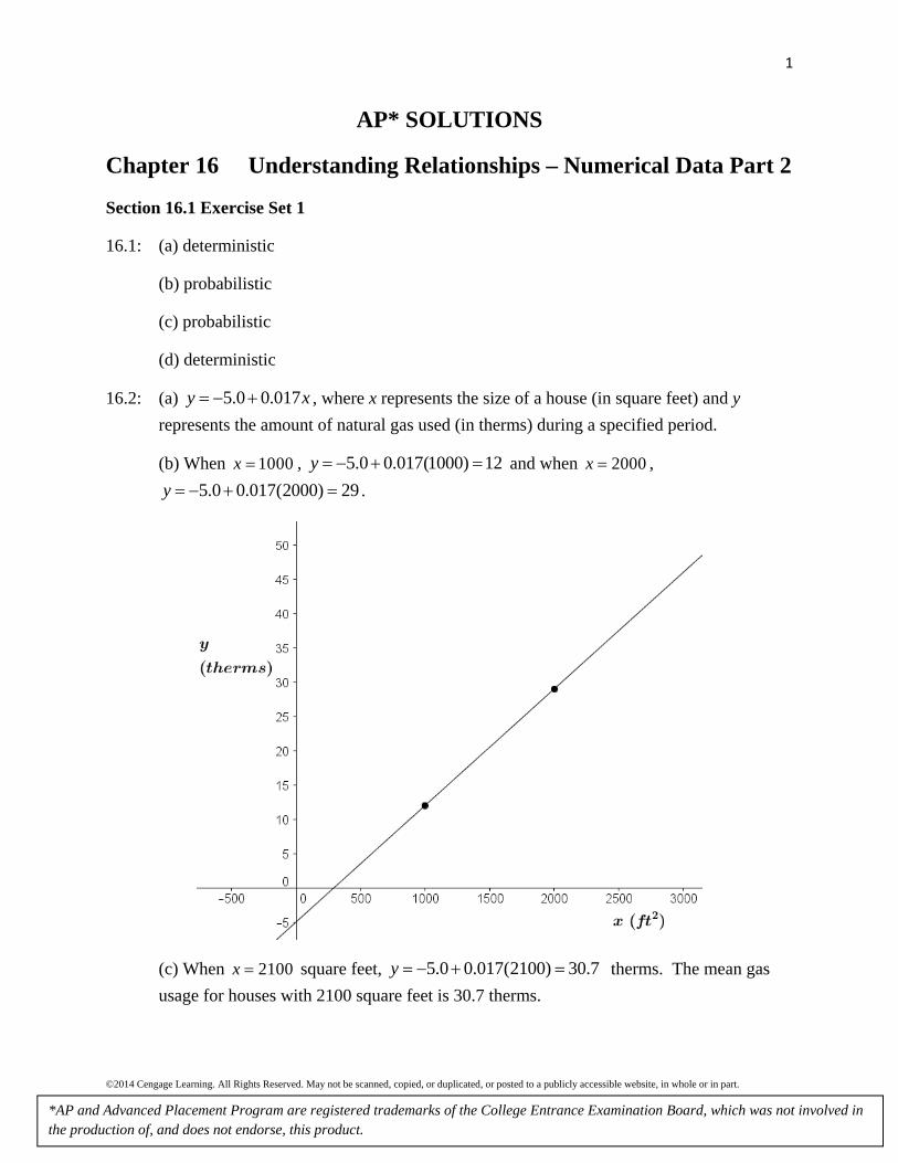
16.2: (a) 5.0 0.017y x , where x represents the size of a house (in square feet) and y

represents the amount of natural gas used (in therms) during a specified period.

(b) When 1000x , 5.0 0.017(1000) 12y and when 2000x ,

5.0 0.017(2000) 29y .

(c) When 2100x square feet, 5.0 0.017(2100) 30.7y therms. The mean gas

usage for houses with 2100 square feet is 30.7 therms.

*AP and Advanced Placement Program are registered trademarks of the College Entrance Examination Board, which was not involved in the production of, and does not endorse, this product.

2


(d) The average change in usage associated with a 1 sq. ft. increase in size is the slope of the population regression line, which is 0.017.

(e) The average change in usage associated with a 100 square foot increase in size is 100(0.017) 1.7 therms.

(f) No, I would not use the model to predict mean usage for a 500 sq. ft. house. The given relationship applies to houses in this community that range between 1000 and 3000 square feet. The house of this size, with 500 square feet lies, outside this range.

16.3: (a) For a 1 square foot increase in house size, the average change in price is $47 (this is the slope of the population regression line). For a 100 square foot increase in house size, the average change in price is $4,700.

(b) When 1,800x square feet, the mean house price (in dollars) is

23,000 47(1,800) 107,600y . The proportion of 1800 square feet homes priced

over $110,000 is 110,000 107,600110,000 ( 0.48) 0.316

5,000P y P z P z

.

The proportion of 1800 square foot homes priced under $100,000 is

100,000 107,600100,000 ( 1.52) 0.064

5,000P y P z P z

.


16.4: (a) probabilistic

(b) deterministic

(c) deterministic

(d) probabilistic

16.5: (a) When 10x inches, the mean flow rate is 0.12 0.095(10) 0.83y . When

15x inches, the mean flow rate is 0.12 0.095(15) 1.305y .

(b) Since the slope of the population regression line is 0.095, the average change in flow rate associated with a 1 inch increase in water pressure drop is 0.095.

16.6: (a) For a 15 mm long quail egg, the mean eggshell thickness is 0.135 0.003(15) 0.18y micrometers. For a 17 mm long quail egg, the mean

eggshell thickness is 0.135 0.003(17) 0.186y micrometers.

3


(b) From part (a), the mean eggshell thickness for a 15 mm long quail egg is 0.18 micrometers. Therefore, the probability that the shell thickness is greater than 0.18 micrometers is ( 0.18) 0.5P y .

(c) The mean eggshell thickness for a 14 mm long quail egg is 0.135 0.003(14) 0.177y micrometers. Therefore, the proportion of quail eggs of

length 14 mm has a shell thickness of greater than 0.175 is

0.175 0.1770.175 ( 0.40) 0.655

0.005P y P z P z

. The proportion of quail

eggs of length 14 mm has a shell thickness of less than 0.178 is

0.178 0.1770.178 ( 0.20) 0.579

0.005P y P z P z

.

Section 16.1 Additional Exercises

16.7: (a) Tom’s pricing model is deterministic because all the customers pay the same amount.

(b) Tom’s pricing strategy is y cx , where y represents the total cost of purchasing x

USB drives at $c each.

(c) Ray’s pricing strategy is y cx e , where y represents the total cost of purchasing x

USB drives at $c each, and e is a random deviation.

(d) The random deviation e will be -2 for about half of the purchases and +1 for about

half of the purchases. The mean of the distribution is 1 1

2 1 0.52 2

and the

standard deviation is 2 21 12 ( 0.5) 1 ( 0.5) 1.5

2 2

.

16.8: (a) probabilistic

(b) deterministic

(c) probabilistic

(d) deterministic

16.9: (a) ˆ 45.573 1.335y x , where y is the predicted breast cancer incidence, and x is the

HRT use.

(b) The slope of the regression line, b = 1.335 cases per 100,000 women, is the estimated average change in breast cancer incidence associated with a 1 percentage point increase in HRT use.

4


(c) The predicted breast cancer incidence when HRT use is 40% is ˆ 45.573 1.335(40) 98.973y , or approximately 99 cases per 100,000 women.

(d) This regression model should not be used to predict breast cancer incidence when HRT use is 20% because that value is outside the range of HRT use values that were used to develop the model. We have no reason to believe that the relationship between HRT use and breast cancer incidence applies outside this range.

(e) 2 0.83r ; This tells us that 83% of the variability in breast cancer incidence can be explained by the linear relationship between breast cancer incidence and HRT use.

(f) 4.154es (obtained using statistical software); The typical amount by which a breast

cancer incidence value deviates from the valued predicted by the least squares regression line is 4.154 cases per 100,000 women.

16.10: (a)

0.110.100.090.080.070.060.050.04

0.14

0.12

0.10

0.08

0.06

0.04

Advertising Share

Mar

ket

Sha

re

Yes, a simple linear regression model is appropriate for describing the relationship between advertising share and market share. The scatterplot shows a linear pattern, and the vertical spread of points does not appear to be changing over the range of x values in the sample. If we assume that the distribution of errors at any given x value is approximately normal, then the simple linear regression model is appropriate.

5


(b) ˆ 0.00227 1.247y x , where y is the predicted market share, and x is the

advertising share. The predicted market share when the advertising share is 0.09 is ˆ 0.00227 1.247(0.09) 0.110y .

(c) 2 0.436r ; This tells us that 43.6% of the variability in market share can be explained by the linear relationship between market share and advertising share.

(d) The point estimate of e is 0.026es (obtained using statistical software). There are

8 degrees of freedom associated with this estimate.

16.11: (a) 2 0.121r

(b) The point estimate of e is 0.155es (this is called the root mean square error in the

JMP computer output). The typical amount by which BMD value deviates from the value in the sample predicted using the least squares regression line is 0.155 g/cm2.

(c) The estimated average change in BMD associated with a 1 kg increase in weight at age 13 is 0.0094363 g/cm2.

(d) The estimated BMD when x = 60 is ˆ 0.5584011 0.0094363(60) 1.1246y g/cm2

16.12: (a) ˆ 3.497 0.1903y x , where y is the predicted embryonic sac diameter (in cm) and

x is the gestational age (in days).

(b) When x = 30, ˆ 3.497 0.1903(30) 2.212y cm

(c) The slope of the least squares regression line, b = 0.1903, is the average change in sac diameter associated with a 1-day increase in gestational age.

(d) Five times the slope of the least squares regression line, 5b = 5(0.1903) = 0.9515, is the average change in sac diameter associated with a 5-day increase in gestational age.

(e) No, the model is not appropriate to make predictions of the mean embryonic sac diameter for all ages from conception to birth because the model was developed using gestational ages of about 24 days to 38 days. There is no guarantee that the observed relationship continues outside that range. This is the danger of extrapolation.

6



16.13: (a) The larger e is, the larger b will be. Because b is in the denominator of the test

statistic, when e is large, the value of the test statistic will tend to be small.

(b) The larger e is, the larger b will be. This means that when e is large the

confidence interval for will tend to be wide.

16.14: (a) The conditions for margin of error are the same as the conditions for a confidence interval, so if a confidence interval was appropriate, no additional conditions are needed.

(b) In order to calculate a margin of error from the reported confidence interval, you would need to know the desired confidence level for the margin of error.

16.15: Both conditions should be rechecked to make sure that they are still reasonable.

16.16: (a) Using the five-step process (HMC3):

Hypotheses:

In the model utility test, the null hypothesis is there is no useful relationship between growth rate from research and development expenditure. The hypotheses are

0 : 0H and : 0aH .

Method:

Because the answers to the four key questions are (Q) hypothesis testing, (S) sample data, (T) two numerical variables in a regression setting, and (N) one sample, a hypothesis test for the slope of a population regression line will be considered. The

test statistic for this test is b

bt

s . A significance level of 0.05 will be used.

Check:

We must check the four basic assumptions. We must assume that the industries sampled are representative of the population of industries, and that they are independent of each other. In addition, the pattern in the scatterplot below looks linear, and the spread does not seem to differ much for different values of x. The boxplot of residuals, also shown below, is not heavily skewed and there are no outliers, so it is reasonable to conclude that the distribution of e is approximately normal.

7


500040003000200010000

4

3

2

1

0

-1

Research and Development Expenditure (thousands of dollars)

Gro

wth

rat

e (%

per

yea

r)

2.01.51.00.50.0-0.5-1.0-1.5Residuals

Calculate:

Computer regression output is shown below:

Predictor Coef SE Coef T P Constant 0.2917 0.5950 0.49 0.641 R&DExp 0.0005751 0.0002518 2.28 0.062

The test statistic is 0.0005751

2.280.0002518b

bt

s . The P-value is twice the area under

the t curve with 6 degrees of freedom, or value 2 ( 2.28) 0.0628P P t . From

the computer output, we also see that the test statistic is 2.28t and the associated P-value is 0.062.

Communicate Results:

Because the P-value of 0.062 is greater than the significance level of 0.05, we fail to reject H0. There is not convincing evidence that the simple linear regression model would provide useful information for predicting growth rate from research and development expenditure.

8


(b) Using the five-step process (EMC3):

Estimate:

The value of , the average change in growth rate associated with a $1000 increase in expenditure will be estimated.

Method:

Because the answers to the four key questions are (Q) estimation, (S) sample data, (T) two numerical variables in a regression setting, and (N) one sample, a confidence interval for b, the slope of the population regression line, will be considered. A 90% confidence level will be used.

Check:

We must check the four basic assumptions. We must assume that the industries sampled are representative of the population of industries, and that they are independent of each other. In addition, the pattern in the scatterplot below looks linear, and the spread does not seem to differ much for different values of x. The boxplot of residuals, also shown below, is not heavily skewed and there are no outliers, so it is reasonable to conclude that the distribution of e is approximately normal.

500040003000200010000

4

3

2

1

0

-1

Research and Development Expenditure (thousands of dollars)

Gro

wth

rat

e (%

per

yea

r)

2.01.51.00.50.0-0.5-1.0-1.5Residuals

9


Calculate:

Computer output is shown below:

Predictor Coef SE Coef T P Constant 0.2917 0.5950 0.49 0.641 R&DExp 0.0005751 0.0002518 2.28 0.062

2 8 2 6df n

The critical t value for a 90% confidence interval and df = 6 is 1.943.

The confidence interval is:

0.0005751 (1.943)(0.0002518)

0.0005751 0.0004892

(critic

(0.0000858,0.00106)

al ) bb t s


Confidence Interval:

You can be 90% confident that the mean change in growth rate associated with a $1000 increase in research and development expenditure is between 0.0000858 and 0.00106.

Confidence Level:

The method used to construct this interval estimate is successful in capturing the actual value of the slope of the population regression line about 90% of the time.


Hypotheses:

In the model utility test, the null hypothesis is there is no useful relationship between

surface angle and typing speed. The hypotheses are 0 : 0H and : 0aH .

Method:

Because the answers to the four key questions are (Q) hypothesis testing, (S) sample data, (T) two numerical variables in a regression setting, and (N) one sample, a

10


hypothesis test for the slope of a population regression line will be considered. The


bt


Check:

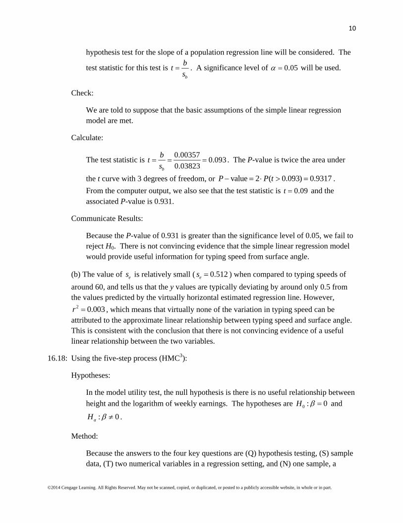
We are told to suppose that the basic assumptions of the simple linear regression model are met.

Calculate:


0.0930.03823b

bt


the t curve with 3 degrees of freedom, or value 2 ( 0.093) 0.9317P P t .

From the computer output, we also see that the test statistic is 0.09t and the associated P-value is 0.931.


Because the P-value of 0.931 is greater than the significance level of 0.05, we fail to reject H0. There is not convincing evidence that the simple linear regression model would provide useful information for typing speed from surface angle.

(b) The value of es is relatively small ( 0.512es ) when compared to typing speeds of

around 60, and tells us that the y values are typically deviating by around only 0.5 from the values predicted by the virtually horizontal estimated regression line. However,

2 0.003r , which means that virtually none of the variation in typing speed can be attributed to the approximate linear relationship between typing speed and surface angle. This is consistent with the conclusion that there is not convincing evidence of a useful linear relationship between the two variables.

16.18: Using the five-step process (HMC3):

Hypotheses:


height and the logarithm of weekly earnings. The hypotheses are 0 : 0H and

: 0aH .

Method:


11




bt


Check:

We are told to suppose that the basic assumptions of the simple linear regression model are met.

Calculate:


5.750.004b

bt

s . Because the sample is very large, we can

use a large number for degrees of freedom. The P-value is twice the area under the t curve, or value 2 ( 5.75) 0P P t .


Because the P-value of approximately 0 is less than the significance level of 0.05, we reject H0. There is convincing evidence of a useful linear relationship between height and the logarithm of weekly earnings.

16.19: (a) By definition, this is the slope of the estimated regression line, or 0.640b g/cm3.

(b) When x = 40, the predicted biomass concentration is ˆ 106.3 0.640(40) 80.7y

g/cm3.

(c) The value of 2r is not very large, indicating that only about 47% of the variability in green biomass concentration can be explained by a linear relationship with elapsed time.


16.20: (a) Rejecting H0 means that there is convincing evidence of a useful linear relationship between x and y.

(b) Failing to reject H0 means that there is not convincing evidence of a useful linear relationship between x and y.

16.21: (a) Using the five-step process (EMC3):

Estimate:

The value of , the mean change in pleasantness rating associated with an increase of 1 impulse per second in firing frequency, will be estimated.

12


Method:


Check:

We must check the four basic assumptions. We must assume that the subjects were either randomly selected or the sample is representative of the population from which they were selected. In addition, the pattern in the scatterplot below looks linear, and the spread does not seem to differ much for different values of x. The boxplot of residuals, also shown below, is not heavily skewed and there are no outliers, so it is reasonable to conclude that the distribution of e is approximately normal.

363432302826242220

3.0

2.5

2.0

1.5

1.0

0.5

0.0

Firing Frequency (impulses per second)

Ple

asan

tnes

s R

atin

g

0.500.250.00-0.25-0.50-0.75Residuals

13


Calculate:


Predictor Coef SE Coef T P Constant -2.3745 0.7454 -3.19 0.013 firing freq 0.14002 0.02568 5.45 0.001

2 10 2 8df n



0.14002 (2.31)(0.02568)

0.14002 0.059

(critic

3

al )

208

(0.081,0.199)

bb t s



You can be 95% confident that the mean change in pleasantness rating associated with an increase of 1 impulse per second in firing frequency is between 0.081 and 0.199.

Confidence Level:


(b) Using the five-step process (HMC3):

Hypotheses:


firing frequency and pleasantness rating. The hypotheses are 0 : 0H and

: 0aH .

Method:


14




bt


Check:

We must check the four basic assumptions. We must assume that the subjects were either randomly selected or the sample is representative of the population from which they were selected. In addition, the pattern in the scatterplot below looks linear, and the spread does not seem to differ much for different values of x. The boxplot of residuals, also shown below, is not heavily skewed and there are no outliers, so it is reasonable to conclude that the distribution of e is approximately normal.

363432302826242220

3.0

2.5

2.0

1.5

1.0

0.5

0.0

Firing Frequency (impulses per second)

Ple

asan

tnes

s R

atin

g

0.500.250.00-0.25-0.50-0.75Residuals

15


Calculate:


Predictor Coef SE Coef T P Constant -2.3745 0.7454 -3.19 0.013 firing freq 0.14002 0.02568 5.45 0.001

2 10 2 8df n


5.450.02568b

bt

s . The P-value is twice the area under the

t curve with 8 degrees of freedom, or value 2 ( 5.45) 0.0006P P t . From the

computer output, we also see that the test statistic is 5.45t and the associated P-value is 0.001.


Because the P-value of 0.001 is less than the significance level of 0.05, we reject H0. There is convincing evidence of a useful linear relationship between firing frequency and pleasantness rating.


Hypotheses:

In the model utility test, the null hypothesis is there is no useful relationship between shrimp catch per tow and oxygen concentration density. The hypotheses are

0 : 0H and : 0aH .

Method:



bt


Check:

We are not given enough information, so we will suppose that the basic assumptions of the simple linear regression model are met.

16


Calculate:


2.8134.63b

bt

s . The P-value is twice the area under the t

curve with 8 degrees of freedom, or value 2 ( 2.81) 0.023P P t . From the



Because the P-value of 0.023 is less than the significance level of 0.05, we reject H0. There is convincing evidence of a useful linear relationship between shrimp catch per tow and oxygen concentration density.

(b) No, the relationship is not strong. The coefficient of determination is 2 0.496r , which indicates that only 49.6% of the variability in catch per tow can be explained by the liner relationship between catch per tow and oxygen concentration density.

(c) Using the five-step process (EMC3):

Estimate:

The value of , the mean change in shrimp catch per tow associated with an increase of 1 unit in oxygen concentration density, will be estimated.

Method:


Check:

We are not given enough information, so we will suppose that the basic assumptions of the simple linear regression model are met.

Calculate:

From the computer output provided, we know that 97.22b and 34.63bs . Given

that the data were collected from 10 sites, we have 8 degrees of freedom. In addition, the critical t value for a 95% confidence interval and df = 8 is 2.31.

17



97.22 (2.31)(34.63)

97.22 79.99

(cr

5

(17.225,177.215

itical

)

) bb t s



You can be 95% confident that the mean change in catch per tow associated with an increase of 1 unit in oxygen concentration density is between 17.225 and 177.215.

Confidence Level:


(d) The margin of error associated with the confidence interval is 79.995.


Hypotheses:


mean childhood blood lead level and brain volume. The hypotheses are 0 : 0H

and : 0aH .

Method:



bt


Check:

We are told to assume that the basic assumptions of the simple linear regression model are met.

18


Calculate:

From the computer output, we see that the test statistic is 3.66t and the associated P-value is 0.000.


Because the P-value of approximately 0 is less than the significance level of 0.05, we reject H0. There is convincing evidence of a useful linear relationship between mean childhood blood lead level and brain volume.


16.24: (a) y x is the equation of the population regression line. y a bx is the

equation of an estimated regression line, which is an estimate of the population regression line based on a sample.

(b) is the slope of the population regression line. b is an estimate of based on a sample.

(c) *x is the mean value of y when *x x . *a bx is an estimate of the mean value

of y (and also a predicted y value) when *x x .

(d) The simple linear regression model assumes that for any fixed value of x, the

distribution of y is normal with mean x and standard deviation . Thus is the

shared standard deviation of these y distributions. The quantity es is an estimate of

obtained from a particular set of (x, y) observations.

16.25: The simple linear regression model assumes that for any fixed value of x, the distribution

of y is normal with mean x and standard deviation . Thus is the shared standard

deviation of these y distributions. The quantity es is an estimate of obtained from a

particular set of (x, y) observations.

16.26: (a) ˆ 96.67 1.59465y x , where y is the predicted mean response time for those

suffering a closed-head injury, and x is the mean response time for individuals with no head injury.

19


(b) Using the five-step process (HMC3):

Hypotheses:

In the model utility test, the null hypothesis is there is no useful relationship between mean response time for individuals with no head injury and the mean response time

for individuals with closed-head injury. The hypotheses are 0 : 0H and

: 0aH .

Method:



bt


Check:

We must check the four basic assumptions. We are told that each observation was based on a different study, and used different subjects, so it is reasonable to assume that the observations are independent. In addition, the pattern in the scatterplot below looks linear, and the spread does not seem to differ much for different values of x. However, the boxplot of residuals, also shown below, is skewed and there are outliers, so it may not be reasonable to conclude that the distribution of e is approximately normal. We shall proceed with caution.

12001000800600400200

2000

1500

1000

500

Mean Response Time - Control

Mea

n R

espo

nse

Tim

e -

CH

I

20


1251007550250-25-50Residuals

Calculate:


Predictor Coef SE Coef T P Constant -96.67 44.30 -2.18 0.061 MRT_control 1.59465 0.05870 27.17 0.000

2 10 2 8df n


27.170.05870b

bt


the t curve with 10 degrees of freedom, or value 2 ( 27.17) 0P P t . From the



Because the P-value of approximately 0 is less than the significance level of 0.05, we reject H0. There is convincing evidence of a useful linear relationship between mean response time for people with no head injury and mean response time for people with a closed-head injury.

16.27: (a) The scatterplot suggests that the simple linear regression model might be appropriate because there is an increasing linear trend in the plot.

(b) ˆ 0.082594 0.0446485y x , where y is the predicted peak photovoltage and x is

the % light absorption.

(c) 2 0.983r

(d) When x = 19.1, ˆ 0.082594 0.0446485(19.1) 0.7702y ;

ˆresidual 0.68 0.770 0.090y y

21


(e) I agree with the author’s assertion of a useful linear relationship between the two variables. Using the five-step process (HMC3):

Hypotheses:


percent light absorption and peak photovoltage. The hypotheses are 0 : 0H and

: 0aH .

Method:



bt


Check:

We must check the four basic assumptions. We are not told how the data were collected or if the observations are independent. We shall proceed as if this is the case. In addition, the pattern in the given scatterplot looks linear, and the spread does not seem to differ much for different values of x. The boxplot of residuals shown below is approximately symmetric and there are outliers, so it is reasonable to conclude that the distribution of e is approximately normal.

0.100.050.00-0.05-0.10Residuals

Calculate:

From the computer output the test statistic is 0.0446485

19.960.002237b

bt

s . The P-

value is twice the area under the t curve with 7 degrees of freedom, or

22


value 2 ( 19.96) 0P P t . From the computer output, we also see that the test

statistic is 19.96t and the associated P-value is < 0.0001.


Because the P-value of approximately 0 is less than the significance level of 0.05, we reject H0. There is convincing evidence of a useful linear relationship between percent light absorption and peak photovoltage.

(f) Using the five-step process (EMC3):

Estimate:

The value of , the average change in peak photovoltage associated with a 1 percentage point increase in light absorption, will be estimated.

Method:

Because the answers to the four key questions are (Q) estimation, (S) sample or experiment data (not directly indicated), (T) two numerical variables in a regression setting, and (N) one sample, a confidence interval for b, the slope of the population regression line, will be considered. A 95% confidence level will be used.

Check:

We must check the four basic assumptions. We are not told how the data were collected or if the observations are independent. We shall proceed as if this is the case. In addition, the pattern in the given scatterplot looks linear, and the spread does not seem to differ much for different values of x. The boxplot of residuals shown below is approximately symmetric and there are outliers, so it is reasonable to conclude that the distribution of e is approximately normal.

0.100.050.00-0.05-0.10Residuals

23


Calculate:

There are 2 9 2 7df n



0.0446485 (2.365)(0.002237)

0.0446485 0.00529

(critic

05

(0.0394,0.0499

l )

)

a bb t s



We are 95% confident that the mean increase in peak photovoltage associated with a 1-percentage point increase in light absorption is between 0.039 and 0.050.

Confidence Level:



Hypotheses:

We want to determine if the new experimental data provide convincing evidence against the prior belief that for each 1-mm increase in chord length, cranial capacity

would be expected to increase by 20 cm3. The hypotheses are 0 : 20H and

: 20aH .

Method:

Because the answers to the four key questions are (Q) hypothesis testing, (S) experiment data, (T) two numerical variables in a regression setting, and (N) one sample, a hypothesis test for the slope of a population regression line will be

considered. The test statistic for this test is 0

b

b bt

s

. A significance level of

0.05 will be used.

24


Check:

We must check the four basic assumptions. We are not told how the data were collected, so we must assume that they were collected appropriately. We must also assume that the observations are independent. In addition, the pattern in the scatterplot below looks linear, and the spread does not seem to differ much for different values of x. The boxplot of residuals, also shown below, is approximately symmetric and there are no outliers, so it may be reasonable to conclude that the distribution of e is approximately normal.

87.585.082.580.077.575.0

1050

1000

950

900

850

800

750

chord length (mm)

cran

ial c

apac

ity

(cub

ic c

enti

met

ers)

100500-50-100Residuals

Calculate:


Predictor Coef SE Coef T P Constant -907.7 407.2 -2.23 0.076 chord length 22.257 5.002 4.45 0.007

2 7 2 5df n

25


The test statistic is 0 22.257 200.451

5.002b

b bt

s

. The P-value is twice the area

under the t curve with 5 degrees of freedom, or -value 2 ( 0.451) 0.671P P t .


Because the P-value of 0.671 is greater than the significance level of 0.05, we fail to reject H0. There is not convincing evidence that the increase in cranial capacity associated with a 1-mm increase in chord length is different from 20 cm3.

16.29: The test statistic for this test is 1

b

bt

s

. From the computer output, b = 0.9797401 and

0.018048bs , so 1 0.9797401 1

1.1230.018048b

bt

s

. The P-value is the area under the t

curve with 44 degrees of freedom, so -value ( 1.123) 0.866P P t . Because the P-

value is greater than any reasonable significance level, the null hypothesis would not be rejected.


16.30: Yes. The pattern in the scatterplot looks linear and the spread around the line does not appear to be changing with x. There is no pattern in the residual plot and the boxplot of the residuals is approximately symmetric and there are no outliers.

16.31: No, it does not appear as if the assumptions of the simple linear regression model are plausible. Although there is an increasing trend in the scatterplot, the relationship is weak and a nonlinear model might fit the data better. This is supported by the curvature shown in the residual plot. Although the normal probability plot is consistent with a normal distribution of the residuals, that alone is not enough to satisfy the assumptions of a simple linear model.

26


16.32: (a)

40035030025020015010050

3

2

1

0

-1

-2

mass

stan

dard

ized

res

idua

l

There is one unusually large standardized residual, 2.52, for the point (164.2, 181). The point (387.8, 310) may be an influential point.

(b) No, the plot seems consistent with the simple linear regression model.

(c) No, it is not reasonable to assume that the variance of y is the same at each x value. The spread of points around the line appears to be different for different values of x.

27


16.33: (a) ˆ 0.9392 0.8731y x , where y is the predicted maximum width in centimeters and x

is the minimum width in centimeters.

(b)

1086420

4

3

2

1

0

-1

Minimum width (cm)

Sta

ndar

dize

d re

sidu

als

The standardized residual plot shows that there is one point that is a clear outlier (the point whose standardized residual is 3.721). This is the point for product 25.

(c) ˆ 0.7029 0.9184y x , where y is the predicted maximum width in centimeters and x

is the minimum width in centimeters. Removal of the point resulted in a reasonably substantial change in the equation of the estimated regression line. Specifically, the y-intercept decreased and the slope increased.

(d) For every 1-cm increase in minimum width, the mean maximum width increases by about 0.9184 cm. It does not make sense to interpret the intercept because it is clearly impossible to have a container whose minimum width is zero.

28


(e) The pattern in the standardized residual plot (shown below) suggests that the variances of the y distributions decrease as x increases, and therefore that the assumption of constant variance is not valid.

1086420

2.0

1.5

1.0

0.5

0.0

-0.5

-1.0

Minimum width (cm)

Sta

ndar

dize

d re

sidu

als

16.34: (a) ˆ 28.516 0.025749y x , where y is the predicted flowering date range, and x is the

elevation. 28.516a , 0.025749b , 2 0.303r , and 4.148es

(b) ˆ 29.371 0.03512y x , where y is the predicted flowering date range, and x is the

elevation. 29.371a , 0.03512b , 2 0.195r , and 4.225es

(c) Deleting the potentially influential data point did not have a big impact on the slope and intercept of the estimated regression line.

(d) I would use the estimated regression equation based on all 19 data points because the regression lines in parts (a) and (b) are not very different from each other (similar slopes and intercepts), and the coefficient of determination (r2) is larger for the regression line in (a) and that line also has a smaller se.


16.35: Yes, the assumptions are plausible. The pattern in the scatterplot looks linear and the spread around the line does not appear to be changing with x. There is no pattern in the residual plot and the normal probability plot of the residuals is reasonably linear

29


16.36: (a) There are no unusual features in the standardized residual plot (plot shown below). The plot supports the assumption that the simple linear regression model applies.

363432302826242220

1.5

1.0

0.5

0.0

-0.5

-1.0

-1.5

-2.0

Firing Frequency

Sta

ndar

dize

d R

esid

ual

(b) Yes, it is reasonable to assume that the error distribution is approximately normal because the normal probability plot shows a roughly linear pattern.

16.37: If the point (20, 33000) is not included, then the slope of the least-squares line would be relatively small and negative. If the point is included then the slope of the least-squares line would still be negative, but much further from zero.

16.38: No, the assumptions of the simple linear regression model are not plausible. The pattern in the scatterplot looks linear, but the spread around the line does not appear to be constant. The histogram of the residuals also appears to be positively skewed.


16.39: (a) There is one point that has a standardized residual of about 2.6. The data point with an x value of about 400 is far away from the rest of the data points in the x direction and might be influential.

(b) No, there is no obvious pattern in the standardized residual plot that would indicate that the simple linear regression model is not appropriate.

(c) No, it is not reasonable to assume that the variance of y is the same at each x value. The spread of points around the line appears to be different for different values of x.

16.40: (a) ˆ 203.85 2.952y x , where y is the predicted mean flowering date range, and x is

the latitude. Therefore, 203.85a and 2.952b . In addition, 2 0.265r and

7.106es .

30


(b) ˆ 436.56 6.861y x , where y is the predicted mean flowering date range, and x is

the latitude. Therefore, 436.56a and 6.861b . In addition, 2 0.543r and

5.803es .

(c) Omitting these two points had a big impact on the values of the intercept and slope of

the least squares regression line, as well as the values of 2r and es . Specifically, the

value of the y-intercept increased from 203.85 to 436.56. The slope also changed dramatically, from -2.952 to -6.861. The value of r 2 increased from 0.265 to 0.543, and the value of se decreased from 7.106 to 5.803.

(d) Using the line for the data that omits the two influential observations would probably be best. Even though you would want to limit predictions to x values in the range 58 to 62, you would expect predictions based on this line to be more accurate due to the increased r 2 value and decreased se.

16.41: Three points that stand out as outliers are those that have residuals of about -30, 30 and 38.

16.42: The approximate coordinates are (38, 2.7).

16.43: (a) The required assumptions are:

(1) The distribution of e at any particular x value has a mean value of 0.

(2) The standard deviation of e is the same for any particular value of x.

(3) The distribution of e at any particular x value is normal.

(4) The random deviations 1 2, , , ne e e associated with different observations are

independent of one another.

31


(b) Yes, the approximately linear pattern in the normal probability plot (shown below) supports the assumption that the distribution of random deviations is normal.

210-1-2

2

1

0

-1

-2

Standardized Residuals

Nor

mal

Sco

re

(c)

22.520.017.515.012.510.07.55.0

2

1

0

-1

-2

Stem Density

Sta

ndar

dize

d R

esid

uals

There are two points with moderately large residuals, specifically, the point (5, 1.20) with a standardized residual of 1.92 and the point (15, 0.00) with a standardized residual of

2.05 .

(d) I have no reason to question the use of the simple linear regression model. Although there are two points with moderately large standardized residuals, the lack of curvature in the residual plot, the approximate constant standard deviation of the residuals, and no apparent influential points all indicate that the simple linear regression model is appropriate.

32


Are You Ready to Move On? Chapter 16 Review Exercises

16.44: A probabilistic model incorporates a random error term; a deterministic model does not.

16.45: and are the intercept and slope, respectively, of the population regression line. a and

b are the least squares estimates of and . e is the standard deviation of e, which is

estimated by se.

16.46: (a) a = 0.5 would be the predicted GPA of a student who scored 0 on the ACT. It is probably not reasonable to interpret the intercept in this model because it is likely that 0 is outside the range of x values used to fit this model.

(b) b = 0.1 represents the change in predicted GPA associated with an increase of 1 in ACT score.

16.47: (a) Yes. The pattern in the scatterplot is approximately linear.

(b) There are no obvious patterns in the residual plot that would indicate that the basic assumptions are not met.

(c) Because the normal probability plot of the residuals is roughly linear, the assumption that the distribution of e is approximately normal is reasonable. However, the boxplot of the residuals contains one outlier, which casts into doubt the assumption of approximate normality.

(d) The large value of r 2 (0.954) combined with the relatively small value for se (0.801) indicate that the linear model fits the data quite well. We know that approximately 95.4% of the variability in body length can be explained by the linear relationship between body length and skull length. In addition, we know that the observations deviate from the least squares regression line by 0.801on average.

16.48: (a) The assumptions are: (1) for any particular value of x, the distribution of e has a mean of 0; (2) the standard deviation of e is the same for each value of x; (3) for any particular value of x, the distribution of e is normal; (4) the e’s are independent of one another.

(b) Assumptions 1, 2, and 3 can be checked using sample data.

(c) Scatterplots and residual plots can be used to check assumptions 1 and 2. Assumption 3 can be checked using a normal probability plot, a boxplot or a histogram.

33



Hypotheses:


brood survival and stem density. The hypotheses are 0 : 0H and : 0aH .

Method:



bt


Check:

We are not given enough information to check the necessary conditions, so we must assume they have all been satisfied.

Calculate:


2.250.011657b

bt

s

. The P-value is twice the area under

the t curve with 21 degrees of freedom, or -value 2 ( 2.25) 0.0353P P t . From

the computer output, we also see that the test statistic is 2.25t and the associated P-value is 0.0355 (slightly different than our computed P-value due to rounding).


Because the P-value of 0.0353 is less than the significance level of 0.05, we reject H0. There is convincing evidence that the simple linear regression model would provide useful information for predicting brood survival from stem density.

(b) The relationship is not strong because 2 0.194r .

(c) Using the five-step process (EMC3):

Estimate:

The value of , the average change in brood survival with an increase of 1000 stems/hectare, will be estimated.

34


Method:


Check:

We are not given enough information to check the necessary conditions, so we must assume they have all been satisfied.

Calculate:

2 23 2 21df n



0.02619 (2.080)(0.011657)

0.02619 0.0242

(

5

critical

( 0.0504, 0.001

9 )

)

4

bb t s



You can be 95% confident that the mean change in brood survival with an increase of 1000 stems/hectare is between -0.0504 and -0.00194.

Confidence Level:


(d) The margin of error associated with the confidence interval in part (c) is 0.02425.

16.50: Two points (the points corresponding to bill overhang values of around 0.35 and 0.40) have large residuals and would be considered outliers. Two other points (the points corresponding to bill overhang values of 0.8 and 1.0) are far removed from the rest of the data set in the x direction and are influential. If these two points were omitted from the data set, the slope of the regression line would be much closer to 0.

35


16.51: The test statistic for this test is 1

b

bt

s

. From the computer output, b = 0.9797401 and

sb = 0.018048, so 1 0.9797401 1

0.01.123

18048b

bt

s

. Regardless of whether the

alternative hypothesis is one-sided or two-sided, the null hypothesis would not be rejected at any reasonable significance level.

Documents

Chapter 16 Understanding Relationships Numerical Data … · Chapter 16 Understanding ... Numerical Data Part 2 Section 16.1 Exercise Set 1 16.1: (a) deterministic (b) ... ©2014