Embed Size (px)
Citation preview

Copyright © 2010, 2007, 2004 Pearson Education, Inc.
Chapter 18
Sampling Distribution
Models

Copyright © 2010, 2007, 2004 Pearson Education, Inc.
Normal Model
When we talk about one data value and the
Normal model we used the notation:
N(μ, σ)
Slide 18 - 3

Copyright © 2010, 2007, 2004 Pearson Education, Inc.
Scenario
Suppose everyone in AP Stats at Geneva High
School took a survey which entailed the question
“Do you believe in ghosts?”
Are the answers received going to be categorical
or quantitative?
Would everyone get the same proportion of
students that said “yes” and “no”?
Why or why not?
Slide 18 - 4

Copyright © 2010, 2007, 2004 Pearson Education, Inc.
Categorical Data
Deals with sample proportions
Slide 18 - 5

Copyright © 2010, 2007, 2004 Pearson Education, Inc. Slide 18 - 6
The Central Limit Theorem for Sample
Proportions
Rather than showing real repeated samples,
imagine what would happen if we were to actually
draw many samples.
Now imagine what would happen if we looked at
the sample proportions for these samples.
The histogram we’d get if we could see all the
proportions from all possible samples is called
the sampling distribution of the proportions.
What would the histogram of all the sample
proportions look like?

Copyright © 2010, 2007, 2004 Pearson Education, Inc. Slide 18 - 7
Modeling the Distribution of
Sample Proportions (cont.)
We would expect the histogram of the sample proportions to center at the true proportion, p, in the population.
As far as the shape of the histogram goes, we can simulate a bunch of random samples that we didn’t really draw.
It turns out that the histogram is unimodal, symmetric, and centered at p.
More specifically, it’s an amazing and fortunate fact that a Normal model is just the right one for the histogram of sample proportions.
Copyright © 2010, 2007, 2004 Pearson Education, Inc. Slide 18 - 8
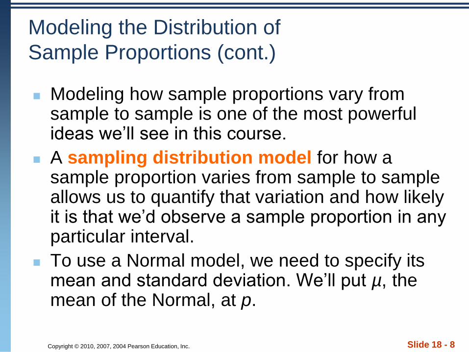
Modeling the Distribution of
Sample Proportions (cont.)
Modeling how sample proportions vary from sample to sample is one of the most powerful ideas we’ll see in this course.
A sampling distribution model for how a sample proportion varies from sample to sample allows us to quantify that variation and how likely it is that we’d observe a sample proportion in any particular interval.
To use a Normal model, we need to specify its mean and standard deviation. We’ll put µ, the mean of the Normal, at p.
Copyright © 2010, 2007, 2004 Pearson Education, Inc. Slide 18 - 9
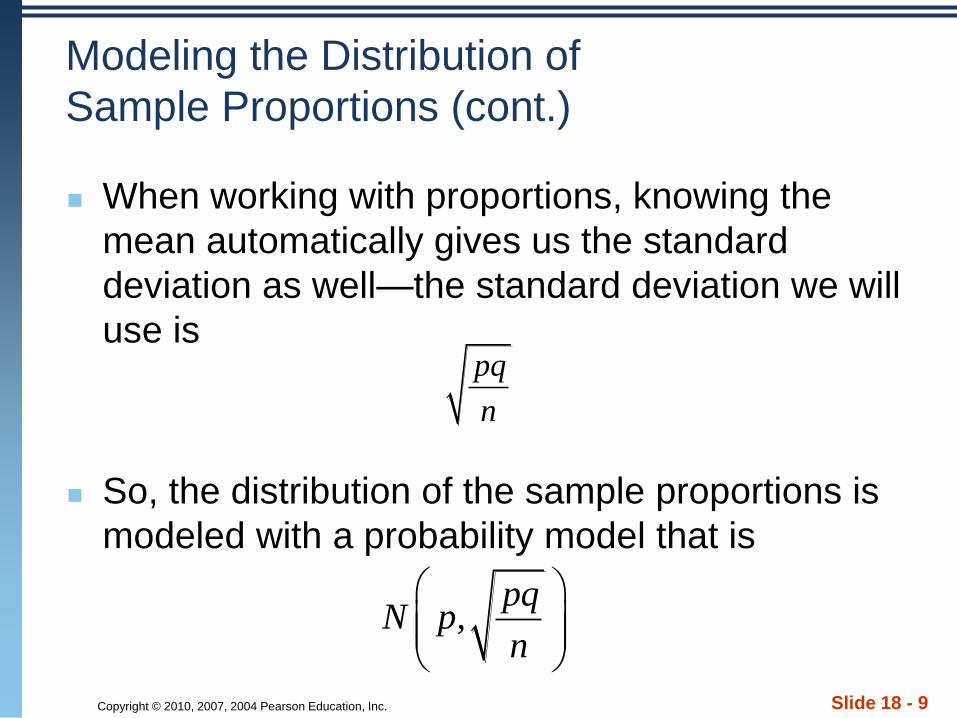
Modeling the Distribution of
Sample Proportions (cont.)
When working with proportions, knowing the
mean automatically gives us the standard
deviation as well—the standard deviation we will
use is
So, the distribution of the sample proportions is
modeled with a probability model that is
,pq
N pn
pq
n

Copyright © 2010, 2007, 2004 Pearson Education, Inc. Slide 18 - 10
Modeling the Distribution of
Sample Proportions (cont.)
A picture of what we just discussed is as follows:

Copyright © 2010, 2007, 2004 Pearson Education, Inc. Slide 18 - 11
Because we have a Normal model, for example, we know that 95% of Normally distributed values are within two standard deviations of the mean.
So we should not be surprised if 95% of various polls gave results that were near the mean but varied above and below that by no more than two standard deviations.
This is what we mean by sampling error. It’s not really an error at all, but just variability you’d expect to see from one sample to another. A better term would be sampling variability.
A reasonable variance/error is ±2σ
The Central Limit Theorem for Sample
Proportions (cont)

Copyright © 2010, 2007, 2004 Pearson Education, Inc. Slide 18 - 12
How Good Is the Normal Model?
The Normal model gets better as a good model
for the distribution of sample proportions as the
sample size gets bigger.
Just how big of a sample do we need? This will
soon be revealed…

Copyright © 2010, 2007, 2004 Pearson Education, Inc. Slide 18 - 13
Assumptions and Conditions
Most models are useful only when specific
assumptions are true.
There are two assumptions in the case of the
model for the distribution of sample proportions:
1. The Independence Assumption: The sampled
values must be independent of each other.
2. The Sample Size Assumption: The sample
size, n, must be large enough.

Copyright © 2010, 2007, 2004 Pearson Education, Inc. Slide 18 - 14
Assumptions and Conditions (cont.)
Assumptions are hard—often impossible—to
check. That’s why we assume them.
Still, we need to check whether the assumptions
are reasonable by checking conditions that
provide information about the assumptions.
The corresponding conditions to check before
using the Normal to model the distribution of
sample proportions are the Randomization
Condition, the 10% Condition and the
Success/Failure Condition.

Copyright © 2010, 2007, 2004 Pearson Education, Inc. Slide 18 - 15
Assumptions and Conditions (cont.)
1. Randomization Condition: The sample should
be a simple random sample of the population.
2. 10% Condition: the sample size, n, must be no
larger than 10% of the population.
3. Success/Failure Condition: The sample size
has to be big enough so that both np (number of
successes) and nq (number of failures) are at
least 10.
…So, we need a large enough sample that is not
too large.

Copyright © 2010, 2007, 2004 Pearson Education, Inc. Slide 18 - 16
A Sampling Distribution Model
for a Proportion A proportion is no longer just a computation from
a set of data.
It is now a random variable quantity that has a probability distribution.
This distribution is called the sampling distribution model for proportions.
Even though we depend on sampling distribution models, we never actually get to see them.
We never actually take repeated samples from the same population and make a histogram. We only imagine or simulate them.

Copyright © 2010, 2007, 2004 Pearson Education, Inc. Slide 18 - 17
A Sampling Distribution Model
for a Proportion (cont.)
Still, sampling distribution models are important
because
they act as a bridge from the real world of data
to the imaginary world of the statistic and
enable us to say something about the
population when all we have is data from the
real world.

Copyright © 2010, 2007, 2004 Pearson Education, Inc. Slide 18 - 18
The Sampling Distribution Model
for a Proportion (cont.)
Provided that the sampled values are
independent and the sample size is large
enough, the sampling distribution of
(sample proportion of success) is modeled
by a Normal model with
Mean:
Standard deviation:
p̂
SD( p̂) pq
n
( p̂) p

Copyright © 2010, 2007, 2004 Pearson Education, Inc.
Example p. 434 #15
Based on past experience, a bank
believes that 7% of the people
who receive loans will not make
payments on time The bank has
recently approved 200 loans.
a) What are the mean and
standard deviation of the
proportion of clients in this
group who may not make timely
payments?
b) What assumptions underlie
you model? Are the conditions
met? Explain.
c) What’s the probability that
over 10% of these clients will
not make timely payments?
Slide 18 - 19

Copyright © 2010, 2007, 2004 Pearson Education, Inc.
Ch 18 Homework
p. 432 #3, 5, 7, 9, 16, 22
Slide 18 - 20

Copyright © 2010, 2007, 2004 Pearson Education, Inc. Slide 18 - 21
What About Quantitative Data?
Proportions summarize categorical variables.
The Normal sampling distribution model looks like
it will be very useful.
Can we do something similar with quantitative
data?
We can indeed. Even more remarkable, not only
can we use all of the same concepts, but almost
the same model.

Copyright © 2010, 2007, 2004 Pearson Education, Inc.
Quantitative Data
Deals with sample means
Slide 18 - 22

Copyright © 2010, 2007, 2004 Pearson Education, Inc. Slide 18 - 23
Simulating the Sampling Distribution of a Mean
Like any statistic computed from a random sample, a sample mean also has a sampling distribution.
We can use simulation to get a sense as to what the sampling distribution of the sample mean might look like…

Copyright © 2010, 2007, 2004 Pearson Education, Inc. Slide 18 - 24
Means – The “Average” of One Die
Let’s start with a simulation of 10,000 tosses of a
die. A histogram of the results is:

Copyright © 2010, 2007, 2004 Pearson Education, Inc. Slide 18 - 25
Means – Averaging More Dice
Looking at the average of
two dice after a simulation
of 10,000 tosses:
The average of three dice
after a simulation of
10,000 tosses looks like:

Copyright © 2010, 2007, 2004 Pearson Education, Inc. Slide 18 - 26
Means – Averaging Still More Dice
The average of 5 dice
after a simulation of
10,000 tosses looks like:
The average of 20 dice
after a simulation of
10,000 tosses looks like:

Copyright © 2010, 2007, 2004 Pearson Education, Inc. Slide 18 - 27
Means – What the Simulations Show
As the sample size (number of dice) gets larger,
each sample average is more likely to be closer
to the population mean.
So, we see the shape continuing to tighten
around 3.5
And, it probably does not shock you that the
sampling distribution of a mean becomes Normal.

Copyright © 2010, 2007, 2004 Pearson Education, Inc. Slide 18 - 28
The Fundamental Theorem of Statistics
The sampling distribution of any mean becomes
more nearly Normal as the sample size grows.
All we need is for the observations to be
independent and collected with randomization.
We don’t even care about the shape of the
population distribution!
The Fundamental Theorem of Statistics is called
the Central Limit Theorem (CLT).
Copyright © 2010, 2007, 2004 Pearson Education, Inc. Slide 18 - 29
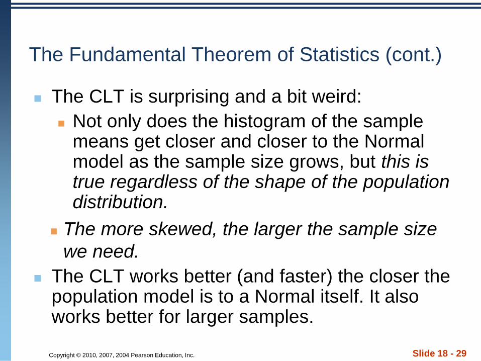
The Fundamental Theorem of Statistics (cont.)
The CLT is surprising and a bit weird:
Not only does the histogram of the sample means get closer and closer to the Normal model as the sample size grows, but this is true regardless of the shape of the population distribution.
The more skewed, the larger the sample size
we need.
The CLT works better (and faster) the closer the population model is to a Normal itself. It also works better for larger samples.

Copyright © 2010, 2007, 2004 Pearson Education, Inc. Slide 18 - 31
Assumptions and Conditions
The CLT requires essentially the same assumptions we saw for modeling proportions:
Independence Assumption: The sampled values must be independent of each other.
Sample Size Assumption: The sample size must be sufficiently large.

Copyright © 2010, 2007, 2004 Pearson Education, Inc. Slide 18 - 32
Assumptions and Conditions (cont.)
We can’t check these directly, but we can think about whether the Independence Assumption is plausible. We can also check some related conditions:
Randomization Condition: The data values must be sampled randomly.
10% Condition: When the sample is drawn without replacement, the sample size, n, should be no more than 10% of the population.
Large Enough Sample Condition: The CLT doesn’t tell us how large a sample we need. For now, you need to think about your sample size in the context of what you know about the population.
Copyright © 2010, 2007, 2004 Pearson Education, Inc. Slide 18 - 33
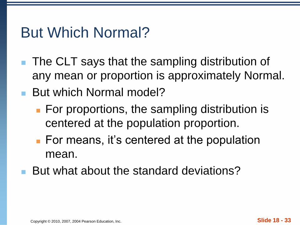
But Which Normal?
The CLT says that the sampling distribution of
any mean or proportion is approximately Normal.
But which Normal model?
For proportions, the sampling distribution is
centered at the population proportion.
For means, it’s centered at the population
mean.
But what about the standard deviations?
Copyright © 2010, 2007, 2004 Pearson Education, Inc. Slide 18 - 34
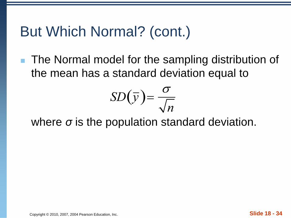
But Which Normal? (cont.)
The Normal model for the sampling distribution of
the mean has a standard deviation equal to
where σ is the population standard deviation.
SD y
n

Copyright © 2010, 2007, 2004 Pearson Education, Inc.
Central Limit Theorem
So the normal model dealing with sample means
is written like…
Slide 18 - 36
),(n
N

Copyright © 2010, 2007, 2004 Pearson Education, Inc. Slide 18 - 37
About Variation
The standard deviation of the sampling
distribution declines only with the square root of
the sample size (the denominator contains the
square root of n).
Therefore, the variability decreases as the sample
size increases.
While we’d always like a larger sample, the
square root limits how much we can make a
sample tell about the population. (This is an
example of the Law of Diminishing Returns.)

Copyright © 2010, 2007, 2004 Pearson Education, Inc.
Example p. 437 #49
A waiter believes the distribution of his tips has a
model that is slightly skewed to the right, with a
mean of $9.60 and a standard deviation of $5.40.
a) Explain why you cannot determine the
probability that a given party will tip him at least
$20.
b) Can you estimate the probability that the
next 4 parties will tip an average of at least $15?
Explain.
c) Is it likely that his 10 parties today will tip an
average of at least $15? Explain.Slide 18 - 38

Copyright © 2010, 2007, 2004 Pearson Education, Inc.
k
Slide 18 - 39

Copyright © 2010, 2007, 2004 Pearson Education, Inc.
Homework
Chapter 18 Homework: p. 432 #31, 33, 37, 50,
Slide 18 - 40

Copyright © 2010, 2007, 2004 Pearson Education, Inc. Slide 18 - 41
The Real World and the Model World
Be careful! Now we have two distributions to deal with.
The first is the real world distribution of the sample, which we might display with a histogram.
The second is the math world sampling distributionof the statistic, which we model with a Normal model based on the Central Limit Theorem.
Don’t confuse the two!

Copyright © 2010, 2007, 2004 Pearson Education, Inc. Slide 18 - 42
Sampling Distribution Models
Always remember that the statistic itself is a
random quantity.
We can’t know what our statistic will be
because it comes from a random sample.
Fortunately, for the mean and proportion, the CLT
tells us that we can model their sampling
distribution directly with a Normal model.

Copyright © 2010, 2007, 2004 Pearson Education, Inc. Slide 18 - 43
Sampling Distribution Models (cont.)
There are two basic truths about sampling distributions:
1. Sampling distributions arise because samples vary. Each random sample will have different cases and, so, a different value of the statistic.
2. Although we can always simulate a sampling distribution, the Central Limit Theorem saves us the trouble for means and proportions.

Copyright © 2010, 2007, 2004 Pearson Education, Inc. Slide 18 - 45
What Can Go Wrong?
Don’t confuse the sampling distribution with the
distribution of the sample.
When you take a sample, you look at the
distribution of the values, usually with a
histogram, and you may calculate summary
statistics.
The sampling distribution is an imaginary
collection of the values that a statistic might
have taken for all random samples—the one
you got and the ones you didn’t get.

Copyright © 2010, 2007, 2004 Pearson Education, Inc. Slide 18 - 46
What Can Go Wrong? (cont.)
Beware of observations that are not independent.
The CLT depends crucially on the assumption
of independence.
You can’t check this with your data—you have
to think about how the data were gathered.
Watch out for small samples from skewed
populations.
The more skewed the distribution, the larger
the sample size we need for the CLT to work.
Copyright © 2010, 2007, 2004 Pearson Education, Inc. Slide 18 - 47
What have we learned?
Sample proportions and means will vary from
sample to sample—that’s sampling error
(sampling variability).
Sampling variability may be unavoidable, but it is
also predictable!

Copyright © 2010, 2007, 2004 Pearson Education, Inc. Slide 18 - 48
What have we learned? (cont.)
We’ve learned to describe the behavior of sample
proportions when our sample is random and large
enough to expect at least 10 successes and
failures.
We’ve also learned to describe the behavior of
sample means (thanks to the CLT!) when our
sample is random (and larger if our data come
from a population that’s not roughly unimodal and
symmetric).

Copyright © 2010, 2007, 2004 Pearson Education, Inc.
Homework
Chapter 18 Homework: p. 432 #2(1), 4(3), 6(5),
8(7), 10(9), 16, 22, 30(29), 34, 38, 50, 52
Slide 18 - 49

Copyright © 2010, 2007, 2004 Pearson Education, Inc.
Example p. 432 #1
See book
Slide 18 - 50

Copyright © 2010, 2007, 2004 Pearson Education, Inc.
Example p. 432 #3
The philanthropic organization in Exercise 1 expects
about a 5% success rate when they send fundraising
letters to the people on their mailing list. In Exercise
1 you looked at the histograms showing distributions
of sample proportions from 1000 simulated mailings
for samples of size 20, 50, 100, and 200. The sample
statistics from each simulation were as follows:
a) According to the CLT,
what should the theoretical
mean and standard
deviation be for these
sample sizes?Slide 18 - 51
n Mean St. Dev
20 0.0497 0.0479
50 0.0516 0.0309
100 0.0497 0.0215
200 0.0501 0.0152

Copyright © 2010, 2007, 2004 Pearson Education, Inc.
Example p. 432 #3
The philanthropic organization in Exercise 1 expects about a 5% success rate when they send fundraising letters to the people on their mailing list. In Exercise 1 you looked at the histograms showing distributions of sample proportions from 1000 simulated mailings for samples of size 20, 50, 100, and 200. The sample statistics from each simulation were as follows:
b) How close are thosetheoretical values to whatwas observed in thesesimulations?
Slide 18 - 52
n Mean St. Dev
20 0.0497 0.0479
50 0.0516 0.0309
100 0.0497 0.0215
200 0.0501 0.0152

Copyright © 2010, 2007, 2004 Pearson Education, Inc.
Example p. 432 #3
The philanthropic organization in Exercise 1 expects about a 5% success rate when they send fundraising letters to the people on their mailing list. In Exercise 1 you looked at the histograms showing distributions of sample proportions from 1000 simulated mailings for samples of size 20, 50, 100, and 200. The sample statistics from each simulation were as follows:
c) Looking at the histogramsin Exercise 1, at what samplesize would you be comfortableusing the Normal modelas an approximation for thesampling distribution?
Slide 18 - 53
n Mean St. Dev
20 0.0497 0.0479
50 0.0516 0.0309
100 0.0497 0.0215
200 0.0501 0.0152

Copyright © 2010, 2007, 2004 Pearson Education, Inc.
Example p. 432 #3
The philanthropic organization in Exercise 1 expects about a 5% success rate when they send fundraising letters to the people on their mailing list. In Exercise 1 you looked at the histograms showing distributions of sample proportions from 1000 simulated mailings for samples of size 20, 50, 100, and 200. The sample statistics from each simulation were as follows:
d) What does theSuccess/Failure Conditionsay about the choice you made in part c?
Slide 18 - 54
n Mean St. Dev
20 0.0497 0.0479
50 0.0516 0.0309
100 0.0497 0.0215
200 0.0501 0.0152

Copyright © 2010, 2007, 2004 Pearson Education, Inc.
Example p. 433 #5
In a large class of introductory Statistics students,
the professor has each person toss a coin 16
times and calculate the proportion of his or her
tosses that were heads. The students then report
their results, and the professor plots a histogram
of these several proportions.
d) Explain why a Normal model should not be
used here.
a) What shape would you expect this histogram
to be? Why?
Slide 18 - 55
Copyright © 2010, 2007, 2004 Pearson Education, Inc.
Example p. 433 #5
In a large class of introductory Statistics students,
the professor has each person toss a coin 16
times and calculate the proportion of his or her
tosses that were heads. The students then report
their results, and the professor plots a histogram
of these several proportions.
b) Where do you expect the histogram to be
centered?
c) How much variability would you expect
among these proportions?
Slide 18 - 56

Copyright © 2010, 2007, 2004 Pearson Education, Inc.
Example p. 433 #7
Suppose the class in Exercise 5 repeats the coin-tossing experiment.
a) The students toss the coins 25 times each. Use the 68-95-99.7 Rule to describe the sampling distribution.
b) Confirm that you can use the Normal model here.
c) They increase the number of tosses to 64 each. Draw and label the appropriate sampling distribution model. Check the appropriate conditions to justify your model.
d) Explain how the sampling distribution model changes as the number of tosses increases.
Slide 18 - 57

Copyright © 2010, 2007, 2004 Pearson Education, Inc.
Example p. 433 #9
One of the students in the introductory Statistics
class in Exercise 7 claims to have tossed her coin
200 times and found only 42% heads. What do
you think of this claim? Explain.
Slide 18 - 58

Copyright © 2010, 2007, 2004 Pearson Education, Inc.
Example p. 434 #21
Just before a referendum on a school budget, a
local newspaper polls 400 random voters in an
attempt to predict whether the budget will pass.
Suppose that the budget actually has the support
of 52% of the voters. What’s the probability the
newspaper’s sample will lead them to predict
defeat (less than 50%)? Be sure to verify that the
assumptions and conditions necessary for our
analysis are met.
Slide 18 - 59

Copyright © 2010, 2007, 2004 Pearson Education, Inc.
Example p. 434 #29
See book
Slide 18 - 60

Copyright © 2010, 2007, 2004 Pearson Education, Inc.
Example p. 432 #31
Researchers measured the Waist Sizes of 250 men in a study on body fat. The true mean and standard deviation of the Waist Sizes for the 250 men are 36.33 in and 4.019 in, respectively. In Exercise 29 you looked at the histograms of simulations that drew samples of sizes 2, 5, 10, and 20 (with replacement). The summary statistics for these simulations were as follows:
a) According to the CLT, what should the theoretical mean and standard deviation be for each ofthese sample sizes?
Slide 18 - 61
n Mean St. Dev
2 36.314 2.855
5 36.314 1.805
10 36.341 1.276
20 36.339 0.895

Copyright © 2010, 2007, 2004 Pearson Education, Inc.
Example p. 432 #31
Researchers measured the Waist Sizes of 250 men in a study on body fat. The true mean and standard deviation of the Waist Sizes for the 250 men are 36.33 in and 4.019 in, respectively. In Exercise 29 you looked at the histograms of simulations that drew samples of sizes 2, 5, 10, and 20 (with replacement). The summary statistics for these simulations were as follows:
b) How close are thosetheoretical values to whatwas observed in thesesimulations?
Slide 18 - 62
n Mean St. Dev
2 36.314 2.855
5 36.314 1.805
10 36.341 1.276
20 36.339 0.895

Copyright © 2010, 2007, 2004 Pearson Education, Inc.
Example p. 432 #31
Researchers measured the Waist Sizes of 250 men in a study on body fat. The true mean and standard deviation of the Waist Sizes for the 250 men are 36.33 in and 4.019 in, respectively. In Exercise 29 you looked at the histograms of simulations that drew samples of sizes 2, 5, 10, and 20 (with replacement). The summary statistics for these simulations were as follows:
c) Looking at the histogramsin Exercise 29, at what sample size would you be comfortable using the Normalmodel as an approximation for the sampling distribution?
Slide 18 - 63
n Mean St. Dev
2 36.314 2.855
5 36.314 1.805
10 36.341 1.276
20 36.339 0.895

Copyright © 2010, 2007, 2004 Pearson Education, Inc.
Example p. 432 #31
Researchers measured the Waist Sizes of 250 men in a study on body fat. The true mean and standard deviation of the Waist Sizes for the 250 men are 36.33 in and 4.019 in, respectively. In Exercise 29 you looked at the histograms of simulations that drew samples of sizes 2, 5, 10, and 20 (with replacement). The summary statistics for these simulations were as follows:
d) What about the shape ofthe distribution of Waist Sizeexplains your choice of sample size in part c?
Slide 18 - 64
n Mean St. Dev
2 36.314 2.855
5 36.314 1.805
10 36.341 1.276
20 36.339 0.895

Copyright © 2010, 2007, 2004 Pearson Education, Inc.
Example p. 436 #33
A college’s data about the incoming freshman
indicates that the mean of their high school GPAs
was 3.4, with a standard deviation of 0.35; the
distribution was roughly mound-shaped and only
slightly skewed. The students are randomly
assigned to freshman writing seminars in groups
of 25. What might the mean GPA of one of these
seminar groups be? Describe the appropriate
sampling distribution model—shape, center,
spread—with attention to assumptions and
conditions. Make a sketch using the 68-95-99.7
Rule.Slide 18 - 65

Copyright © 2010, 2007, 2004 Pearson Education, Inc.
Example p. 437 #49
A waiter believes the distribution of his tips has a
model that is slightly skewed to the right, with a
mean of $9.60 and a standard deviation of $5.40.
a) Explain why you cannot determine the
probability that a given party will tip him at least
$20.
b) Can you estimate the probability that the
next 4 parties will tip an average of at least $15?
Explain.
c) Is it likely that his 10 parties today will tip an
average of at least $15? Explain.Slide 18 - 66

Copyright © 2010, 2007, 2004 Pearson Education, Inc.
k
Slide 18 - 67

Copyright © 2010, 2007, 2004 Pearson Education, Inc.
Example p. 438 #51
A waiter believes the distribution of his tips has a
model that is slightly skewed to the right, with a
mean of $9.60 and a standard deviation of $5.40.
The waiter usually waits on about 40 parties over
a weekend of work.
a) Estimate the probability that he will earn at
least $500 in tips.
b) How much does he earn on the best 10% of
such weekends?
Slide 18 - 68

Copyright © 2010, 2007, 2004 Pearson Education, Inc.
Homework
Chapter 18 Homework: p. 432 #2(1), 4(3), 6(5),
8(7), 10(9), 16, 22, 30(29), 32(31), 34, 38, 50(49),
52(51)
Slide 18 - 69

Copyright © 2010, 2007, 2004 Pearson Education, Inc.
Practice 1
“Groovy” M&M’s are supposed to make up 30% of
the candies sold. In a large bag of 250 M&M’s,
what is the probability that we get at least 25%
groovy candies?
Slide 18 - 70

Copyright © 2010, 2007, 2004 Pearson Education, Inc.
Practice 2
At birth, babies average 7.8 pounds, with a
standard deviation of 2.1 pounds. A random
sample of 34 babies born to mothers living near a
large factory that may be polluting the air and
water shows a mean birth weight of only 7.2
pounds. Is that unusually low? Explain.
Slide 18 - 71