Embed Size (px)
Citation preview

Chapter 2
An Overview of Isotope Geochemistry in EnvironmentalStudies
D. Porcelli and M. Baskaran
Abstract Isotopes of many elements have been used
in terrestrial, atmospheric, and aqueous environmental
studies, providing powerful tracers and rate monitors.
Short-lived nuclides that can be used to measure time
are continuously produced from nuclear reactions
involving cosmic rays, both within the atmosphere
and exposed surfaces, and from decay of long-lived
isotopes. Nuclear activities have produced various iso-
topes that can be used as atmospheric and ocean circu-
lation tracers. Production of radiogenic nuclides from
decay of long-lived nuclides generates widespread
distinctive isotopic compositions in rocks and soils
that can be used to identify the sources of ores and
trace water circulation patterns. Variations in isotope
ratios are also generated as isotopes are fractionated
between chemical species, and the extent of fraction-
ation can be used to identify the specific chemical
processes involved. A number of different techniques
are used to separate and measure isotopes of interest
depending upon the half-life of the isotopes, the ratios
of the stable isotopes of the element, and the overall
abundance of the isotopes available for analysis.
Future progress in the field will follow developments
in analytical instrumentation and in the creative
exploitation of isotopic tools to new applications.
2.1 Introduction
Isotope geochemistry is a discipline central to envi-
ronmental studies, providing dating methods, tracers,
rate information, and fingerprints for chemical pro-
cesses in almost every setting. There are 75 elements
that have useful isotopes in this respect, and so there is
a large array of isotopic methods potentially available.
The field has grown dramatically as the technological
means have been developed for measuring small var-
iations in the abundance of specific isotopes, and the
ratios of isotopes with increasing precision.
Most elements have several naturally occurring
isotopes, as the number of neutrons that can form a
stable or long-lived nucleus can vary, and the relative
abundances of these isotopes can be very different.
Every element also has isotopes that contain neutrons
in a quantity that render them unstable. While most
have exceedingly short half-lives and are only seen
under artificial conditions (>80% of the 2,500 nuclides),
there are many that are produced by naturally-occurring
processes and have sufficiently long half-lives to be
present in the environment in measurable quantities.
Such production involves nuclear reactions, either the
decay of parent isotopes, the interactions of stable
nuclides with natural fluxes of subatomic particles in
the environment, or the reactions occurring in nuclear
reactors or nuclear detonations. The isotopes thus
produced provide the basis for most methods for
obtaining absolute ages and information on the rates
of environmental processes. Their decay follows the
well-known radioactive decay law (first-order kinet-
ics), where the fraction of atoms, l (the decay con-
stant), that decay over a period of time is fixed and an
intrinsic characteristic of the isotope:
D. Porcelli (*)
Department of Earth Sciences, Oxford University, South Parks
Road, Oxford OX1 3AN, UK
e‐mail: [email protected]
M. Baskaran
Department of Geology, Wayne State University, Detroit, MI
48202, USA
e‐mail: [email protected]
M. Baskaran (ed.), Handbook of Environmental Isotope Geochemistry, Advances in Isotope Geochemistry,
DOI 10.1007/978-3-642-10637-8_2, # Springer-Verlag Berlin Heidelberg 2011
11

dN
dt¼ � lN: (2.1)
When an isotope is incorporated and subsequently
isolated in an environmental material with no
exchange with surroundings and no additional produc-
tion, the abundance changes only due to radioactive
decay, and (2.1) can be integrated to describe the
resulting isotope abundance with time;
N ¼ N0e�lt: (2.2)
The decay constant is related to the well-known
half-life (t1=2) by the relationship:
l ¼ ln 2
t1=2¼ 0:693
t1=2: (2.3)
This equation provides the basis for all absolute
dating methodologies. However, individual methods
may involve considering further factors, such as
continuing production within the material, open system
behaviour, or the accumulation of daughter isotopes.
The radionuclides undergo radioactive decay by alpha,
beta (negatron and positron) or electron capture. The
elements that have radioactive isotopes, or isotopic var-
iations due to radioactive decay, are shown in Fig. 2.1.
Variations in stable isotopes also occur, as the
slight differences in mass between the different iso-
topes lead to slightly different bond strengths that
affect the partitioning between different chemical spe-
cies and the adsorption of ions. Isotope variations
therefore provide a fingerprint of the processes that
have affected an element. While the isotope variations
of H, O, and C have been widely used to understand
the cycles of water and carbon, relatively recent
advances in instrumentation has made it possible to
precisely measure the variations in other elements, and
the potential information that can be obtained has yet
to be fully exploited. The full range of elements with
multiple isotopes is shown in Fig. 2.2.
One consideration for assessing the feasibility of
obtaining isotopic measurements is the amount of an
element available. Note that it is not necessarily the
concentrations that are a limitation, but the absolute
amount, since elements can be concentrated from
whatever mass is necessary- although of course there
are considerations of difficulty of separation, sample
availability and blanks. For example, it is not difficult
to filter very large volumes of air, or to concentrate
constituents from relatively large amounts of water,
but the dissolution of large silicate rock samples is
more involved. In response to difficulties in present
methods or the challenges of new applications, new
methods for the separation of the elements of interest
from different materials are being constantly devel-
oped. Overall, analyses can be performed not only on
major elements, but even elements that are trace con-
stituents; e.g. very pure materials (99.999% pure) still
contain constituents in concentrations of micrograms
Fig. 2.1 Elements with isotopes that can be used in environ-
mental studies and are anthropogenic, cosmogenic (produced
either in the atmosphere or within exposedmaterials), radiogenic
(from production of long-lived isotopes), or that are part of the
U- or Th-decay series
12 D. Porcelli and M. Baskaran

per gram (ppm) and so are amenable to analysis.
Further considerations of the abundances that can be
measured are discussed below.
The following sections provide a general guide to
the range of isotopes available, and the most wide-
spread uses in the terrestrial environment. It is not
meant to be exhaustive, as there are many innovative
uses of isotopes, but rather indicative of the sorts of
problems can be approached, and what isotopic tools
are available for particular question. More details
about the most commonly used methods, as well as
the most innovative new applications, are reported
elsewhere in this volume. Section 2.3 provides a
brief survey of the analytical methods available.
2.2 Applications of Isotopesin the Environment
In the following sections, applications of isotopes to
environmental problems are presented according to
the different sources of radioactive isotopes and
causes of variations in stable isotopes.
2.2.1 Atmospheric Short-Lived Nuclides
A range of isotopes is produced from reactions involv-
ing cosmic rays, largely protons, which bombard the
Earth from space. The interactions between these cos-
mic rays and atmospheric gases produce a suite of
radionuclides with half-lives ranging from less than a
second to more than a million years (see list in Lal and
Baskaran 2011). There are a number of nuclides that
have sufficiently long half-lives to then enter into
environmental cycles in various ways (see Table 2.1).
The best-known nuclide is 14C, which forms CO2 after
its production and then is incorporated into organic
matter or dissolves into the oceans. With a half-life of
5730a, it can be used to date material that incorporates
this 14CO2, from plant material, calcium carbonate
(including corals), to circulating ocean waters. Infor-
mation can also be obtained regarding rates of
exchange between reservoirs with different 14C/12C
ratios, and biogeochemical cycling of C and associated
elements. Other nuclides are removed from the atmo-
sphere by scavenging onto aerosols and removed by
precipitation, and can provide information on the rates
of atmospheric removal. By entering into surface
waters and sediments, these nuclides also serve as
environmental tracers. For example, there are two
isotopes produced of the particle-reactive element
Be, 7Be (t1/2 ¼ 53.3 days) and 10Be (1.4Ma). The
distribution of 7Be/10Be ratios, combined with data
on the spatial variations in the flux of Be isotopes to
the Earth’s surface, can be used to quantify processes
such as stratospheric-tropospheric exchange of air
masses, atmospheric circulation, and the removal rate
Fig. 2.2 The elements that have stable isotope variations useful
for environmental studies. The shaded elements do not have
more than one isotope that is stable and not radiogenic. While
all others potentially can display stable isotope variations, sig-
nificant isotopic variations in the environment have been docu-
mented for the circled elements
2 An Overview of Isotope Geochemistry in Environmental Studies 13

of aerosols (see Lal and Baskaran 2011). The record of
Be in ice cores and sediments on the continents can be
used to determine past Be fluxes as well as to quantify
sources of sediments, rates of sediment accumulation
and mixing (see Du et al. 2011; Kaste and Baskaran
2011). Other isotopes, with different half-lives or dif-
ferent scavenging characteristics, provide comple-
mentary constraints on atmospheric and sedimentary
processes (Table 2.1).
A number of isotopes are produced in the atmo-
sphere from the decay of 222Rn, which is produced
within rocks and soils from decay of 226Ra, and then
released into the atmosphere. The daughter products of222Rn (mainly 210Pb (22.3a) and 210Po (138 days)) that
are produced in the atmosphere have been used as
tracers to identify the sources of aerosols and their
residence times in the atmosphere (Kim et al. 2011;
Baskaran 2011). Furthermore, 210Pb adheres to parti-
cles that are delivered to the Earth’s surface at a
relatively constant rate and are deposited in sediments,
and its subsequent decay provides a widely used
method for determining the age of sediments and so
the rates of sedimentation.
A number of isotopes are incorporated into the hydro-
logic cycle and so providemeans for dating groundwaters.
This includes the noble gases 39Ar (t1/2 ¼ 268a), 81Kr
(230ka) and 3H (Kulongoski and Hilton 2011)
which dissolve into waters and then provide ideal
tracers that do not interact with aquifer rocks and so
travel conservatively with groundwater, but are pres-
ent in such low concentrations that their measurement
has proven to be difficult. The isotope 129I (16Ma)
readily dissolves and also behaves conservatively:
with such a long half-life, however, it is only useful
for very old groundwater systems. The readily ana-
lyzed 14C also has been used for dating groundwater,
but the 14C/12C ratio changes not only because of
decay of 14C, but also through a number of other
processes such as interaction with C-bearing minerals
such as calcium carbonate; therefore, more detailed
modelling is required to obtain a reliable age.
General reviews on the use of isotopes produced
in the atmosphere for determining soil erosion and
sedimentation rates, and for providing constraints in
hydrological studies, are provided by Lal (1991, 1999)
and Phillips and Castro (2003).
2.2.2 Cosmogenic Nuclides in Solids
Cosmogenic nuclides are formed not just within the
atmosphere, but also in solids at the Earth’s surface,
and so can be used to date materials based only upon
exposure history, rather than reflecting the time of
formation or of specific chemical interactions. The
cosmic particles that have escaped interaction within
the atmosphere penetrate into rocks for up to a few
meters, and interact with a range of target elements to
generate nuclear reactions through neutron capture,
muon capture, and spallation (emission of various
fragments). From the present concentration and the
production rate, an age for the exposure of that surface
to cosmic rays can be readily calculated (Lal 1991).
A wide range of nuclides is produced, although only
a few are produced in detectable amounts, are
sufficiently long-lived, and are not naturally present
in concentrations that overwhelm additions from cos-
mic ray interactions. An additional complexity in
Table 2.1 Atmospheric radionuclides
Isotope Half-life Common applications3H 12.32a Dating of groundwater, mixing of water
masses, diffusion rates7Be 53.3 day Atmospheric scavenging, atmospheric
circulation, vertical mixing of water,
soil erosion studies10Be 1.4 � 106a Dating of sediments, growth rates of Mn
nodules, soil erosion study,
stratosphere-troposphere exchange,
residence time of aerosols14C 5730a Atmospheric circulation, dating of
sediments, tracing of C cycling in
reservoirs, dating groundwater32Si 140a Atmospheric circulation, Si cycling in the
ocean32P 25.3 day Atmospheric circulation, tracing oceanic
P pool33P 14.3 day35S 87 day Cycling of S in the atmosphere39Ar 268a Atmospheric circulation and air-sea
exchange81Kr 2.3 � 105a Dating of groundwater129I 1.6 � 107a Dating of groundwater210Pb 22.3a Dating, deposition velocity of aerosols,
sources of air masses, soil erosion,
sediment focusing
Selected isotopes generated within the atmosphere that have
been used for environmental studies, along with some common
applications. All isotopes are produced by nuclear reactions in
the atmosphere induced by cosmic radiation, with the exception
of 210Pb, which is produced by decay of 222Rn released from
the surface
14 D. Porcelli and M. Baskaran

obtaining ages from this method is that production
rates must be well known, and considerable research
has been devoted to their determination. These are
dependent upon target characteristics, including the
concentration of target isotopes, the depth of burial,
and the angle of exposure, as well as factors affecting
the intensity of the incident cosmic radiation, including
altitude and geomagnetic latitude. Also, development
of these methods has been coupled to advances in
analytical capabilities that have made it possible to
measure the small number of atoms involved. It is
the high resolution available from accelerator mass
spectrometry (see Sect. 2.3.2) that has made it possible
to do this in the presence of other isotopes of the same
element that are present in quantities that are many
orders of magnitude greater.
The most commonly used cosmogenic nuclides are
listed in Table 2.2 (see also Fig. 2.3). These include
several stable isotopes, 3He and 21Ne, which accumu-
late continuously within materials. In contrast, the
radioactive isotopes 10Be, 14C, 26Al, and 36Cl will
continue to increase until a steady state concentration
is reached in which the constant production rate is
matched by the decay rate (which is proportional to
the concentration). While this state is approached
asymptotically, in practice within ~5 half-lives con-
centration changes are no longer resolvable. At this
Table 2.2 Widely used cosmogenic nuclides in solids
Isotope Primary targets Half-life Commonly dated
materials10Be O, Mg, Fe 1.4Ma Quartz, olivine,
magnetite26Al Si, Al, Fe 705ka Quartz, olivine36Cl Ca, K, Cl 301ka Quartz3He O, Mg, Si, Ca, Fe, Al Stable Olivine, pyroxene21Ne Mg, Na, Al, Fe, Si Stable Quartz, olivine,
pyroxene
The most commonly used isotopes that are produced by interac-
tion of cosmic rays the primary target elements listed
Fig. 2.3 The 238U, 235U, and 232Th decay series. The presence of the series of short-lived nuclides throughout the environment is
due to their continuous production by long-lived parents
2 An Overview of Isotope Geochemistry in Environmental Studies 15

point, no further time information is gained; such
samples can then be assigned only a minimum age.
There have been a considerable number of applica-
tions of these methods, which have proven invaluable
to the understanding of recent surface events. There are
a number of reviews available, including those by
Niedermann (2002), which focuses on 3He and 21Ne,
and Gosse and Phillips (2001). A full description of the
methods and applications is given by Dunai (2010).
Some of the obvious targets for obtaining simple expo-
sure ages are lava flows, material exposed by land-
slides, and archaeological surfaces. Meteorite impacts
have been dated by obtaining exposure ages of exca-
vated material, and the timing of glacial retreats has
been constrained by dating boulders in glacial mor-
aines and glacial erratics. The ages of the oldest sur-
faces in dry environments where little erosion occurs
have also been obtained. Movement on faults has been
studied by measuring samples along fault scarps to
obtain the rate at which the fault face was exposed.
Cosmogenic nuclides have also been used for under-
standing landscape evolution (see review by Cockburn
and Summerfield 2004) and erosion rates (Lal 1991). In
this case, the production rate with depth must be known
and coupled with an erosion history, usually assumed to
occur at a constant rate. The concentrations of samples
at the surface (or any depth) are then the result of the
production rate over the time that the sample has
approached the surface due to erosion andwas subjected
to progressively increasing production. The calculations
are somewhat involved, since production rates due to
neutron capture, muon reactions, and spallation have
different depth dependencies, and the use of several
different cosmogenic nuclides can provide better con-
straints (Lal 2011). Overall, plausible rates have been
obtained for erosion, which had hitherto been very
difficult to constrain. The same principle has been
applied to studies of regional rates of erosion by mea-
suring 10Be in surface material that has been gathered
in rivers (Schaller et al. 2001), and this has provided
key data for regional landscape evolution studies
(Willenbring and von Blanckenburg 2010).
2.2.3 Decay Series Nuclides
The very long-lived nuclides 238U, 235U, and 232Th
decay to sequences of short-lived nuclides that
eventually lead to stable Pb isotopes (see Fig. 2.3
and Table 2.3). The decay of these parents thus sup-
ports a continuous definable supply of short-lived
nuclides in the environment that can be exploited for
environmental studies, especially for determining ages
and rates over a range of timescales from days to
hundreds of thousands of years. The abundance of
each isotope is controlled by that of its parent, and
since this dependence continues up the chain, the
connections between the isotopes can lead to consid-
erable complexity in calculating the evolution of some
daughters. However, since the isotopes represent a
wide range of elements with very different geochemi-
cal behaviours, such connections also present a wealth
of opportunities for short-term geochronology and
Table 2.3 Decay series nuclides used in environmental studies
Isotope Half-life Common applications238U 4.468 � 109a Dating, tracing sources of U234U 2.445 � 104a Dating of carbonates, tracing sources
of water232Th 1.405 � 1010a Quantifying lithogenic component in
aqueous system, atmosphere230Th 7.538 � 104a Dating, scavenging, ventilation of
water mass234Th 24.1 day Particle cycling, POC export, rates of
sediment mixing228Th 1.913a Particle scavenging and tracer for
other particulate pollutants227Th 18.72 day Particle tracer231Pa 3.276 � 104a Dating, sedimentation rates,
scavenging228Ra 5.75a Tracing water masses, vertical and
horizontal mixing rates226Ra 1600a Dating, water mass tracing, rates of
mixing224Ra 3.66 day Residence time of coastal waters,
mixing of shallow waters223Ra 11.435 day Residence time of coastal waters,
mixing of shallow waters227Ac 21.773a Dating, scavenging222Rn 3.82 day Gas exchange, vertical and horizontal
diffusion210Pb 22.3a Dating (e.g. carbonates, sediments, ice
cores, aerosols, artwork); sediment
mixing, focusing and erosion;
scavenging; resuspension210Po 138 day Carbon export, remineralization,
particle cycling in marine
environment
Radioactive isotopes within the 238U, 235U, and 232Th decay
series that have been directly applied to environmental studies.
The remaining isotopes within the decay series are generally too
short-lived to provide useful environmental information and are
simply present in activities equal to those of their parents
16 D. Porcelli and M. Baskaran

environmental rate studies (see several papers in Iva-
novich and Harmon 1992; Baskaran 2011).
The abundance of a short-lived nuclide is conve-
niently reported as an activity (¼ Nl, i.e. the abun-
dance times the decay constant), which is equal to the
decay rate (dN/dt). In any sample that has been undis-
turbed for a long period (>~1.5 Ma), the activities of
all of the isotopes in each decay chain are equal to that
of the long-lived parent element, in what is referred to
as secular equilibrium. In this case, the ratios of the
abundances of all the daughter isotopes are clearly
defined, and the distribution of all the isotopes in a
decay chain is controlled by the distribution of the
long-lived parent. Unweathered bedrock provides an
example where secular equilibrium could be expected
to occur. However, the different isotopes can be sepa-
rated by a number of processes. The different chemical
properties of the elements can lead to different mobi-
lities under different environmental conditions. Ura-
nium is relatively soluble under oxidizing conditions,
and so is readily transported in groundwaters and
surface waters. Thorium, Pa and Pb are insoluble and
highly reactive with surfaces of soil grains and aquifer
rocks, and adsorb onto particles in the water column.
Radium is also readily adsorbed in freshwaters, but not
in highly saline waters where it is displaced by com-
peting ions. Radon is a noble gas, and so is not surface-
reactive and is the most mobile.
Isotopes in the decay series can also be separated
from one another by the physical process of recoil.
During alpha decay, a sufficient amount of energy
is released to propel alpha particles a considerable
distance, while the daughter isotope is recoiled in
the opposite direction several hundred Angstroms
(depending upon the decay energy and the matrix).
When this recoil sends an atom across a material’s
surface, it leads to the release of the atom. This is the
dominant process releasing short-lived nuclides into
groundwater, as well as releasing Rn from source
rocks. This mechanism therefore can separate short-
lived daughter nuclides from the long-lived parent of
the decay series. It can also separate the products of
alpha decay from those of beta decay, which is not
sufficiently energetic to result in substantial recoil. For
example, waters typically have (234U/238U) activity
ratios that are greater than the secular equilibrium
ratio of that found in crustal rocks, due to the prefer-
ential release of 234U by recoil.
A more detailed discussion of the equations
describing the production and decay of the intermedi-
ate daughters of the decay series is included in Appen-
dix 2. In general, where an intermediate isotope is
isolated from its parent, it decays according to (2.2).
Where the activity ratio of daughter to parent is shifted
from the secular equilibrium value of 1, the ratio will
evolve back to the same activity as its parent through
either decay of the excess daughter, or grow-in of the
daughter back to secular equilibrium (Baskaran 2011).
These features form the basis for dating recently pro-
duced materials. In addition, U- and Th- series system-
atics can be used to understand dynamic processes,
where the isotopes are continuously supplied and
removed by physical or chemical processes as well
as by decay (e.g. Vigier and Bourdon 2011).
The U-Th series radionuclides have a wide range of
applications throughout the environmental sciences.
Recent reviews cover those related to nuclides in the
atmosphere (Church and Sarin 2008; Baskaran 2010;
Hirose 2011), in weathering profiles and surface
waters (Chabaux et al. 2003; Cochran and Masque
2003; Swarzenski et al. 2003), and in groundwater
(Porcelli and Swarzenski 2003; Porcelli 2008). Recent
materials that incorporate nuclides in ratios that do not
reflect secular equilibrium (due either to discrimina-
tion during uptake or availability of the nuclides) can
be dated, including biogenic and inorganic carbonates
from marine and terrestrial environments that readily
take up U and Ra but not Th or Pb, and sediments from
marine and lacustrine systems that accumulate sinking
sediments enriched in particle-reactive elements like
Th and Pb (Baskaran 2011). The migration rates of U-
Th-series radionuclides can be constrained where
continuing fractionation between parent and daughter
isotopes occurs. These rates can then be related to
broader processes, such as physical and chemical ero-
sion rates as well as water-rock interaction in ground-
water systems, where soluble from insoluble nuclides
are separated (Vigier and Bourdon 2011). Also,
the effects of particles in the atmosphere and water
column can be assessed from the removal rates of
particle-reactive nuclides (Kim et al. 2011).
2.2.4 Anthropogenic Isotopes
Anthropogenic isotopes are generated through nuclear
reactions created under the unusual circumstances of
high energies and high atomic particle fluxes, either
within nuclear reactors or during nuclear weapons
2 An Overview of Isotope Geochemistry in Environmental Studies 17

explosions. These are certainly of concern as contami-
nants in the environment, but also provide tools for
environmental studies, often representing clear signals
from defined sources. These include radionuclides not
otherwise present in the environment that can there-
fore be clearly traced at low concentrations (e.g. 137Cs,239,240Pu; Hong et al. 2011; Ketterer et al. 2011), as
well as distinct pulses of otherwise naturally-occurring
species (e.g. 14C). There is a very wide range of iso-
topes that have been produced by such sources, but
many of these are too short-lived or do not provide a
sufficiently large signal over natural background con-
centrations to be of widespread use in environmental
studies. Those that have found broader application are
listed in Table 2.4.
The release of radioactive nuclides into the envi-
ronment from reactors, as well as from nuclear waste
reprocessing and storage facilities, can occur in a
number of ways. Discharges through airborne efflu-
ents can widely disperse the isotopes over a large area
and enter soils and the hydrological cycle through
fallout, as observed for the Chernobyl release in
1986. Discharges of water effluents, including cooling
and process waters, can be followed from these point
sources in circulating waters, such as from the Sella-
field nuclear processing and power plant, which
released radionuclides (e.g. 137Cs, 134Cs, 129I) from
the western coast of England into the Irish Sea and
which can be traced high into the Arctic Ocean (dis-
cussed in Hong et al. 2011). Leaks into the ground
from storage and processing facilities can also release
radionuclides that are transported in groundwater, at
locations such as the Hanford nuclear production facil-
ity in Washington State. At the Nevada Test Site, Pu
was found to have migrated >1 km, facilitated by
transport on colloids. Releases by all of these mechan-
isms at lower levels have been documented around
many reactor facilities. Even where levels are too
low to pose a health concern, the isotopes can be
readily measured and their sources identified. Trans-
uranics are also utilized as tracers for investigating soil
erosion, transport and deposition in the environment
(Ketterer et al. 2011; Matisoff and Whiting 2011).
As discussed above, cosmic rays entering the atmo-
sphere cause nuclear reactions that produce a number
of radioisotopes. Atmospheric bomb testing, which
peaked in the late 1950s and diminished dramatically
after 1963, produced a spike in the production of some
of these radionuclides (e.g. 14C), and high atmospheric
concentrations have persisted due to long atmospheric
residence times or continuing fluxes from nuclear
activities. These higher concentrations can then be
used as markers to identify younger materials. The
most widely used isotopes in this category are 3H
and 14C. There are a number of others, including85Kr (10.72a), 129I (15.7Ma), and 36Cl (3.0 � 105a)
Table 2.4 Anthropogenic isotopes most commonly used in environmental studies
Isotope Half-life Main sources Examples of major uses Notes3H 12.32a Bomb testing Tracing rainwater from time of bomb peak
in ground waters and seawater
Background cosmogenic 3H
Reactors Ages determined using 3H-3He14C 5730a Bomb testing Identifying organic and inorganic carbonate
materials produced in last 60 years
Background cosmogenic 14C
54Mn 312 day Bomb testing Trophic transfer in organisms No background137Cs,134Cs
30.14a bomb testing, reactors,
reprocessing plants
Tracing seawater, soil erosion, sediment
dating and mixing, sources of aerosols
No background
90Sr 28.6a Reactors, bomb testing Tracing seawater, sources of dust No background239Pu 24100a Reactors, bomb testing Tracing seawater, identifying sources of Pu,
sediment dating, soil erosion, tracing
atmospheric dust
No naturally-occurring Pu240Pu 6560a241Pu 14.4a131I 8.02 day129I 1.57 � 107a Bomb testing, reactors Dating groundwater, water mass movements Background cosmogenic 129I85Kr 10.72a Bomb testing Dating groundwater36Cl 3.0 � 105a Bomb testing Dating groundwater Background cosmogenic 36Cl241Am 432.2a Reactors Tracing sources of Am No naturally-occurring Am
The anthropogenic isotopes that can be used as point source tracers, or provide global markers of the time of formation of
environmental materials
18 D. Porcelli and M. Baskaran

that have not been as widely applied, partly because
they require difficult analyses. For a discussion of a
number of applications, see Phillips and Castro (2003).
For the anthropogenic radionuclides that have half-
lives that are long compared to the times since their
release, time information can be derived from know-
ing the time of nuclide production, e.g. the present
distribution of an isotope provides information on the
rate of transport since production or discharge. An
exception to this is 3H, which has a half-life of only
12.3 years and decays to the rare stable isotope 3He.
By measuring both of these isotopes, time information
can be obtained, e.g. 3H-3He ages for groundwaters,
which measure the time since rainwater incorporating
atmospheric 3H has entered the aquifer (Kulongoski
and Hilton 2011).
2.2.5 Radiogenic Isotopes
There are a number of radioactive isotopes with half-
lives that are useful for understanding geological time-
scales, but do not change significantly over periods of
interest in environmental studies. However, these iso-
topes have produced substantial variations in the iso-
topes of the elements that have daughter isotopes. The
resulting isotopic signatures in rocks, sediments, and
ores have been exploited in environmental studies. An
example is the Rb-Sr system, which is the most com-
monly used. The long-term decay of 87Rb produces87Sr, and so the abundance of this isotope, relative to a
stable isotope of Sr such as 86Sr, varies according to
the equation:
87Sr86Sr
¼87Sr86Sr
� �0
þ87Rb86Sr
el87t � 1� �
; (2.4)
where the (87Sr/86Sr)0 ratio is the initial isotope ratio
and l87 is the decay constant of 87Rb. Clearly, the
present 87Sr/86Sr ratio is greater for samples that have
greater ages, t, and samples with larger Rb/Sr ratios.
The 87Sr/86Sr ratio therefore varies between different
rock types and formations. Since Rb is an alkali metal
and Sr is an alkaline earth, these elements behave
differently in geological processes, creating large var-
iations in Rb/Sr, and so large variations in 87Sr/86Sr.
The 87Sr/86Sr ratio has been shown to vary widely in
surface rocks, and so any Sr released into soils, rivers,
and groundwaters has an isotopic signature that reflects
its source. Changes in local sources can also be identi-
fied; for example, Keller et al. (2010) identified thaw-
ing of permafrost from the changes in stream water87Sr/86Sr ratio as tills with greater amounts of carbon-
ate deeper in soil profiles were weathered. Strontium
isotopes have been used as tracers for identifying
populations of migratory birds and fish in streams and
rivers (Kennedy et al. 1997; Chamberlain et al. 1997)
as well as in archaeology (Slovak and Paytan 2011). Sr
isotopes have also been used to trace agricultural pro-
ducts, which have incorporated Sr, along with Ca, from
soils incorporating Sr isotope ratios of the underlying
rocks. The sources and transport of dust across the
globe have been traced using the isotopic compositions
of Sr, Nd, and Pb (Grousset and Biscaye 2005). Varia-
tions in the Pb isotopic ratios between environmental
samples (soil, aerosols, household paint, household
dust, and water samples in house) and children’s
blood have been utilized to identify and quantify the
sources of blood Pb in children (Gulson 2011).
Other isotope systems that can be used for similar
purposes are listed in Table 2.5. In each case, chemical
differences between the chemical behaviour of the
parent and daughter isotopes have led to variations in
their ratio over geological timescales, and so identifi-
able variations in the environment can be exploited for
tracing. The most obvious differences are often
regional, as reflected in the isotopic compositions in
rivers, especially for Sr and Nd. More local studies can
identify different rocks, or even separate minerals,
involved in weathering or contributing to waters
(Tripathy et al. 2011). Using this information, ground-
water flow paths and the sources of inorganic consti-
tuents can be deduced.
2.2.6 Stable Isotopes
In addition to variations in isotope ratios produced by
the production or decay of nuclides due to nuclear
processes, there are variations in the distribution of
other isotopes between different phases or chemical
species. These are subtle, as isotopes of an element
still behave in fundamentally the same way, but the
slight variations in atomic mass result in differences in
bonding and kinetics. This is due to differences in
vibrational energies reflecting differences in the
masses of atoms, since the vibrational frequency of a
2 An Overview of Isotope Geochemistry in Environmental Studies 19
molecule is directly proportional to the forces that
hold atoms together, such as electron arrangements,
nuclear charges and the positions of the atoms in the
molecule, and inversely proportional to the masses of
the atoms. The result is stable isotope fractionation,
which is generally considered only for isotopes that
are neither radioactive nor radiogenic, since variations
in these isotopes often cannot be readily separated
from decay effects. While studies of such fractiona-
tions were originally confined to light elements (e.g.
H, O, N, S), isotopic variations have now been found
even in the heavy stable elements Tl (Rehkamper and
Halliday 1999) and U (Stirling et al. 2007), and so
across the entire periodic table.
The difference in the ratio of two isotopes of the
same element in species or phases A (RA) and B (RB)
can be described by a fractionation factor a
a ¼ RA
RB
: (2.5)
Fractionation between isotopes of the same element
generally appear to be linear; e.g. the ratio of isotopes
two mass units apart will be fractionated twice as
much as the ratio of elements one mass unit apart
(mass dependent fractionation). Since the changes in
isotopic values are generally very small, values are
typically given as parts per thousand (permil) devia-
tions from a standard; e.g. for example, for O,
d18Osample¼18O 16O
�� �sample
� 18O 16O�� �
standard
18O 16O=ð Þstandard�103:
(2.6)
Therefore, results are reported relative to a standard.
In some cases, however, several standards are in use,
especially when analytical procedures are being devel-
oped, making comparisons between datasets difficult.
In those caseswhere smaller variations can bemeasured
precisely, values are given in parts per 104 (as e values).When the isotopic composition of two phases in equi-
librium are measured, the difference between them can
be related to the fractionation factor by
d18OA � d18OB � a� 1ð Þ � 103: (2.7)
Therefore, the fractionation factor between two
phases can be obtained by measuring the differ-
ence in isotopic composition between phases in
equilibrium.
Schauble (2004) provides a summary of the general
patterns seen in equilibrium isotope fractionation.
Fractionation effects are largest for low mass ele-
ments, and scale according to the difference in atomic
masses of two isotopes relative to the average mass of
the element squared, i.e. Dm/m2. Heavy isotopes will
favour species in which the element has the stiffest
bonds. In environmental systems, this includes bonds
of metals with the highest oxidation state, those with a
bond partner with a high oxidation state, and bonds
with anions with low atomic number (including
organic ligands).
Fractionation can occur not only by equilibrium
partitioning, but also due to kinetic processes. This
includes transport phenomena such as diffusion,
where lighter isotopes have higher velocities
(inversely proportional to the square root of atomic/
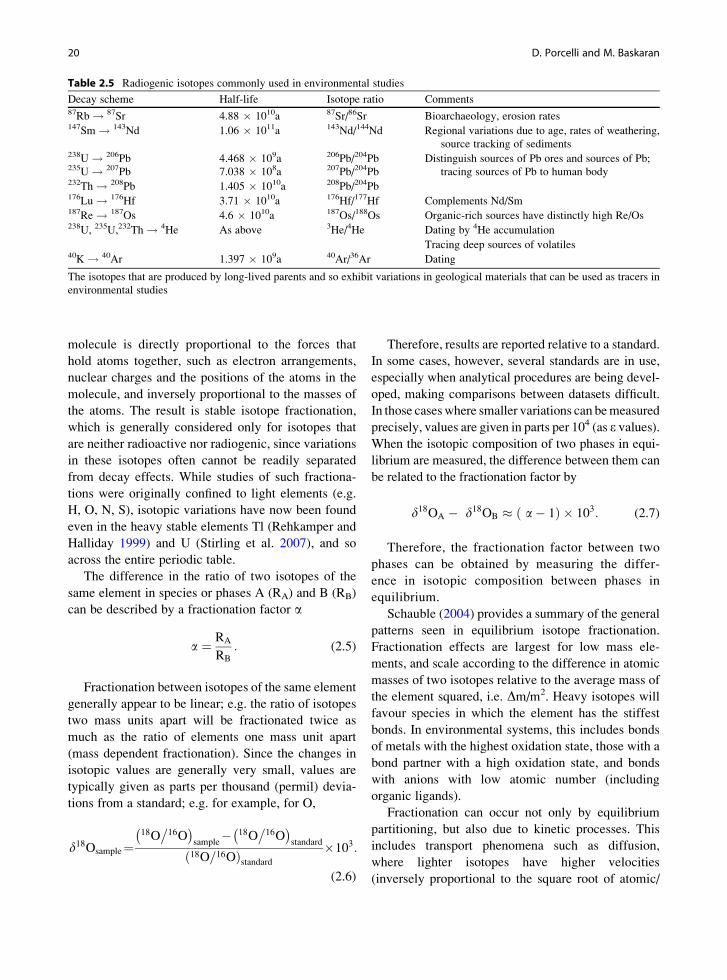
Table 2.5 Radiogenic isotopes commonly used in environmental studies
Decay scheme Half-life Isotope ratio Comments87Rb ! 87Sr 4.88 � 1010a 87Sr/86Sr Bioarchaeology, erosion rates147Sm ! 143Nd 1.06 � 1011a 143Nd/144Nd Regional variations due to age, rates of weathering,
source tracking of sediments238U ! 206Pb 4.468 � 109a 206Pb/204Pb Distinguish sources of Pb ores and sources of Pb;
tracing sources of Pb to human body235U ! 207Pb 7.038 � 108a 207Pb/204Pb232Th ! 208Pb 1.405 � 1010a 208Pb/204Pb176Lu ! 176Hf 3.71 � 1010a 176Hf/177Hf Complements Nd/Sm187Re ! 187Os 4.6 � 1010a 187Os/188Os Organic-rich sources have distinctly high Re/Os238U, 235U,232Th ! 4He As above 3He/4He Dating by 4He accumulation
Tracing deep sources of volatiles40K ! 40Ar 1.397 � 109a 40Ar/36Ar Dating
The isotopes that are produced by long-lived parents and so exhibit variations in geological materials that can be used as tracers in
environmental studies
20 D. Porcelli and M. Baskaran

molecular weight) that generate fractionation over dif-
fusive gradients. This can also be due to reaction
kinetics related to the strength of bonding, where ligh-
ter isotopes have bonds that can be broken more read-
ily and so can be enriched in reactants. This can be
seen in many biological processes, where uptake of
elements can involve pathways involving multiple
reactions and so considerable fractionation. It is
important to note that it is not always possible to
determine if equilibrium or kinetic fractionation is
occurring; while laboratory experiments often endeav-
our to ensure equilibrium is reached, it is not always
clear in the natural environment. Also, where kinetic
fractionation is produced in a regular fashion, for
example due to microbial reduction, it may not be
easily distinguished from inorganic equilibrium frac-
tionation processes
When the isotopes of an element are distributed
between two separate phases or species in equilibrium,
then the difference in isotope ratio is determined by
(2.7). However, the absolute ratio of each is deter-
mined by mass balance according to the simple mixing
equation
RTotal ¼ RAfA þ RBð1� fAÞ: (2.8)
For example, as shown in Fig. 2.4, if an element is
partitioned between two phases, and the mixture is
almost entirely composed of phase A, then that phase
will have the ratio close to that of the total mixture,
while the ratio of phase B will be offset by the frac-
tionation factor. If the mixture is almost entirely com-
posed of phase B, it is the composition of phase A that
will be offset from the bulk. Intermediate values of
R for each phase will reflect the balance between the
two phases according to (2.8). Such batch partitioning
is more likely to apply where both forms are entirely
open to chemical exchange, e.g. two different species
in solution.
Often equilibrium is not maintained between a
chemical species or phase and the source reservoir. In
this case, the isotopic composition of the source evolves
according to Rayleigh distillation, in which a small
increment of a phase or species is formed in equilibrium
with the source, but is immediately removed from fur-
ther interaction, and so does not remain in equilibrium
with the changing source. For example, crystals preci-
pitating from solution are unlikely to continue reacting
with the solution. If the source originally had an isotope
ratio R0, and the isotopes of an element of interest are
fractionated with material being removed according to
Fig. 2.4 An example of stable isotope fractionation. (a) When
Hg is partitioned between two phases, isotopic fractionation can
occur; the heavier isotopes are preferentially incorporated into
phase B, so that a(198Hg/202Hg)A ¼ (198Hg/202Hg)B. Fraction-
ation between all the isotopes is generally linear, i.e. the extent
of fractionation between any two isotopes is proportional to the
mass difference between them. (b) If there is equilibrium batch
partitioning between A and B, then there is a difference of a
between both phases, and the specific composition of each
depends upon mass balance; e.g. if there is very little of phases
A, then the ratio of phase B is about equal to the bulk value,
while phase A has a value that is a times higher. (c) If there iscontinuous removal of phase B, so that only each increment
being removed is in equilibrium with phase A, then this process
of Rayleigh distillation will drive the isotopic composition of A
to more extreme compositions than a batch process
2 An Overview of Isotope Geochemistry in Environmental Studies 21

a fractionation factor a, then when in total a fraction f ofthe element has been removed, the integrated effect will
be to generate a ratio RA in the source according to the
equation:
RA
R0
¼ f a�1ð Þ: (2.9)
This is illustrated in Fig. 2.4; once a significant
amount of an element has been removed, the ratio of
the source has changed to a greater degree than by
batch partitioning, and more extreme ratios can be
obtained when f approaches 1 (most of the element
has been removed). As long as the same fractionation
factor affects each increment, (2.9) will describe the
evolution of the solution, whether the fractionation is
due to equilibrium or kinetic fractionation. Such evo-
lution is likely to apply where solid phases are formed
from solution, where water-rock interaction occurs,
and where biological uptake occurs.
While fractionation between isotopes of an element
is generally mass dependent, i.e. proportional to the
mass deference between any two isotopes, there are a
few circumstances where mass-independent fraction-
ation is observed and a number of theories have been
proposed to explain this phenomenon. Examples
include O isotopes in stratospheric and tropospheric
ozone (due to rotational energies of asymmetric mole-
cules; Gao and Marcus 2001), S in Archean sediments
(possibly from S photo-dissociated in the early atmo-
sphere; Farquhar et al. 2000), and Hg isotopes involved
in photochemical reactions in the environment (due to
nuclear volume and magnetic isotope effects; see
Blum 2011). These provide an added dimension for
diagnosing the processes affecting these elements.
A wide range of applications has been explored for
stable isotope fractionations. Oxygen isotopes vary in
precipitation, and have been used as a hydrological
tracer, while C, S, and N have been used to trace
biogeochemical cycles (see e.g. reviews in Kendall
and McDonnell 1998) and tracers of human diet
(Chesson et al. 2011; Schwarcz and Schoeninger
2011). Isotopic variations in Li, Mg, and Sr have been
related to adsorption and incorporation in clays, and so
can be used to understand weathering and trace element
migration (Burton and Vigier 2011; Reynolds 2011).
Various metals with multiple redox states, including Fe,
Cr, U,Mo, Ni, Cu, Zn, Cd, Hg, Se, and Tl, have isotopic
variations that have been used to understand redox
processes in present and past environments (see the
four papers by Bullen 2011; Johnson 2011; Nielsen
and Rehk€amper 2011; Rehk€amper et al. 2011).
Stable isotopes can also be used in understanding
environmental contamination. Chemical processing can
generate isotopic differences in industrial products that
provide a means for identifying sources. For example,
C and Cl isotope differences have been found between
different manufacturers of chlorinated solvents (van
Warmerdam et al. 1995) and this can be used to trace
contaminant migration. It has also been shown that
degradation of these compounds can fractionate Cl iso-
topes, so that the extent of degradation can be deter-
mined (Sturchio et al. 1998, 2011). As another example,
Cr isotopes are fractionated in groundwaters when Cr is
reduced to a less soluble species, and so decreases in
concentrations due to dilution can be distinguished
from decreases due to precipitation (Ellis et al. 2002).
Other examples of documented isotope variations
that have been used to understand environmental pro-
cesses are listed in Table 2.6. Measurements are all
made using mass spectrometry. Samples are corrected
for instrumental fractionation using either comparison
with standards in gas-source mass spectrometry and
ICPMS, or using a double spike and TIMS and ICPMS
(see below).
2.3 Measurement Techniques
There are two fundamental approaches to measuring
the abundance of isotopes. Radioactive isotopes can be
measured by quantifying the radiation resulting from
decay, and then relating the decay rate to the abun-
dance using (2.1). A number of these counting meth-
ods are widely used, especially for short-lived
nuclides. Alternatively, atoms of any isotope can be
directly measured by mass spectrometry, which sepa-
rates ions according to mass followed by direct count-
ing. These methods typically involve greater
investment in instrumentation, but can often detect
more subtle variations. The techniques are discussed
further in the following sections.
2.3.1 Counting Methods
There are a number of techniques available for the
detection of alpha, beta, and gamma radiation that
22 D. Porcelli and M. Baskaran

can be applied depending upon the mode and energy
of decay, as well as the emission spectrum that is
produced. In some circumstances, an isotope will
decay to another short-lived isotope that can be more
readily measured and then related to the abundance of
the parent (e.g. 210Pb using 210Po measured by alpha
spectrometry or 226Ra using 214Pb or 214Bi measured
by gamma spectrometry).
Following is a brief description of the different
analytical methods available. For many isotopes,
there are several measurement options, and the best
method is determined by the type of sample, the abun-
dance of the isotope of interest, and the precision
required. A more extensive review is given by Hou
and Roos (2008).
2.3.1.1 Alpha Spectrometry
Isotopes that are subject to alpha decay can be
measured by detecting and counting the emitted
alpha particles. Contributions from the decay of other
Table 2.6 Commonly used stable isotopes
Element Typical reported
ratio
Examples of applications
H 2H/1H (D/H) Tracing both production and
origin of food, groundwater
sources
Li 6Li/7Li Weathering processes,
adsorption of Li in aquifers
B 10B/9B
C 13C/12C Tracing both production and
origin of food, paleodiet
reconstruction, hydrocarbon
exploration, environmental
forensics
N 15N/14N N cycling, tracing both
production and origin of
food
O 18O/16O Tracing both production and
origin of food, sulphate and
nitrate cycle in the
atmosphere and aqueous
system, oxidation pathways
of compounds, paleo-
climate (air temperature,
humidity and amounts of
precipitation), sources of
groundwater
Mg 26Mg/24Mg Lithological studies, adsorption
of Mg in aquifers
Si 30Si/28Si Global Si cycle, weathering
rates, biogeochemical
cycling of Si
S 34S/32S Sulfur cycling in the
atmosphere, sources of S in
the environment
Cl 37Cl/35Cl Forensics, source tracking of
organochlorine and
inorganic chlorate,
fractionation in deep brines
Ca 44Ca/40Ca Vertebrate paleodiet tracer,
biogeochemical pathways
of Ca
Cr 53Cr/52Cr Source tracking of Cr
contamination, Cr reduction
Fe 56Fe/54Fe Fe redox cycling, Fe
incorporation in aquifers
Ni 60Ni/58Ni Sources and transport of Ni;
methanogenesis
Cu 65Cu/63Cu Sources and transport of Cu;
partitioning of Cu between
ligand-bound dissolved and
particulate phases
Zn 66Zn/64Zn Transport of Zn along cell walls
of xylem; micronutrient
transport in plants; pathways
of anthropogenic Zn
Se 80Se/76Se Redox reactions
Sr 88Sr/86Sr Sr adsorption in aquifers
(continued)
Table 2.6 (continued)
Element Typical reported
ratio
Examples of applications
Mo 97Mo/94Mo Sources, transport of Mo, paleo-
redox changes in aqueous
system
Cd 114Cd/110Cd,112Cd/110Cd
Paleo-ocenography,
reconstruction of past
nutrient levels in seawater
Os 187Os/188Os Tracking anthropogenic and
weathering sources of Os
Mo 97Mo/95Mo Redox reactions
Hg 202Hg/198Hg,199Hg/198Hg,201Hg/198Hg
Forensics, sources tracking,
reaction pathways of Hg
using both mass-dependent
and mass-independent
fractionation
Tl 205Tl/203Tl Paleoinput of Fe and Mn,
hydrothermal fluid flux
Pb 206Pb/204Pb,207Pb/204Pb,208Pb/204Pb
Source identification of Pb in
metals, tracing pathways
of Pb to human system,
tracing dust
Po 210Po POC export, reminerlization of
particles, biogenic particle
cycling
U 238U/235U Depleted/enriched uranium
identification, redox
2 An Overview of Isotope Geochemistry in Environmental Studies 23

isotopes can be distinguished by alpha particle
energy, although there is overlap between alpha ener-
gies emitted by some of the nuclides. However,
practical difficulties arise due to the interaction of
alpha particles with atoms of other species that are
loaded in the source along with the sample. This can
cause a spread in particle energies and so reduce the
energy resolution of the alpha spectrum, making the
data often unusable. Therefore, good chemical sepa-
ration and purification from other elements is critical,
and the isotope of interest must be then deposited
as a thin layer to minimize adsorption by the
element of interest iteself (self-shielding). This is
done by electroplating onto metal discs or by sorbing
onto thin MnO2 layers. Accurate determination of
the concentration of these isotopes requires careful
control of chemical yields during processing as well
as of counter efficiency. A detailed review of the
chemical procedures adopted for measuring alpha-
emitting radionuclides in the U-Th-series is given
in Lally (1992).
A number of detectors have been utilized for
alpha measurements that include ionization cham-
bers, proportional counters, scintillation detectors
(plastic and liquid), and semiconductor detectors.
Of these, the semiconductors (in particular, surface
barrier and ion-implanted silicon detectors) have
been the most widely used detectors due to their
superior energy resolution and relatively high count-
ing efficiency (typically 30% for a 450-mm2 surface-
barrier detector). More detailed comparison of the
various types of detector material is given in Hou
and Roos (2008).
The very low background of alpha detectors
(0.8–2 counts for a particular isotope per day), rela-
tively high efficiency (~30% for 450 mm2 surface
area detectors) and very good energy resolution
(about 17–20 keV for 5.1 MeV) lead to detection
limits of 0.010–0.025 mBq (where Bq, a Becquerel,
is a decay per second); this can be related to an
abundance using (2.1), so that, e.g. for a 1 � 105
year half-life radionuclide this corresponds to as
little as 0.08 femtomoles. While the long preparation
times associated with chemical separation, purifica-
tion, electroplating and counting impose a practical
constraint on sample throughput, the relatively low-
cost of alpha spectrometers and their maintenance
is an advantage.
2.3.1.2 Beta Spectrometry
For isotopes that are subject to beta decay, abundances
can be measured by detecting and counting the beta
particles (electrons) that are emitted. The most com-
mon detector is a Geiger-M€uller (GM) counter, which
employs a gas-filled tube where atoms are ionized
by each intercepted beta particle, and this is converted
into an electrical pulse. Background signals from cos-
mic rays are reduced through shielding and anti-
coincidence counters, which subtract counts that
correspond to detections of high-energy particles
entering the counting chamber.
Although adsorption by surrounding atoms is not as
efficient as for alpha particles, it is still significant, and
so samples are often deposited as thin sources onto a
metal disc to increase counting efficiencies. Also, fil-
ters that contain particles collected from air and water
samples can be measured directly. Dissolved species
of particle-reactive elements (e.g. Th) can be concen-
trated from large water volumes by scavenging onto
precipitated Fe or Mn oxides that are then collected
onto filters. These filters can be analyzed directly
(Rutgers van der Loeff and Moore 1999).
It should be noted that GM counters do not distin-
guish between beta particles by energy, and so cannot
separate contributions from different isotopes through
the energy spectrum. While isotopes can often be
isolated by chemical separation, some elements have
several isotopes and some isotopes have short-lived
beta-emitting daughter isotopes that are continuously
produced. In these cases, multiple counting can be
done to identify and quantify different isotopes based
upon their different half-lives. Also, selective absor-
bers of various thicknesses between the source and
counter can be used to suppress interference from
isotopes that produce lower energy beta particles.
The counting efficiency of a GM counter varies
depending on the thickness of the source and on
counter properties. One of the commonly used GM
counters, the Risø Counter (Risø National Laboratory,
Roskilde, Denmark), has a typical efficiency of ~40%
for most commonly occurring beta–emitting radionu-
clides. A typical background of this anti-coincidence
counter, with 10 cm of lead shielding, is 0.15–0.20
counts per minute, corresponding to ~0.8 mBq. This
can be compared to the detection limit for an alpha-
emitting radionuclide; the background of a new
24 D. Porcelli and M. Baskaran

alpha detector is 0.03–0.09 counts per hour, which
corresponds to 0.03–0.08 mBq (at ~30% counting
efficiency). Thus, the detection limit in alpha spec-
trometry is more than an order of magnitude higher
than that of beta spectrometry.
The GM counter is not suitable for analyzing iso-
topes such as 3H and 14C that emit low-energy
(~200 keV) electrons, which are adsorbed in the detec-
tor window. For these nuclides, a liquid scintillation
counter (LSC) is used, in which a sample is dissolved
in a solvent solution containing compounds that con-
vert energy received from each beta particle into light,
and the resulting pulses are counted. This method has
minimal self-adsorption and relatively easy sample
preparation, and can be used for all beta-emitters.
However, background count rates are substantially
higher than in GM counters.
2.3.1.3 Gamma Spectrometry
Alpha and beta-emitting radionuclides often decay to
atoms in excited energy states, which then reach the
ground state by emitting gamma radiation at discrete
characteristic energies. Gamma rays can be detected
when they ionize target atoms, so that the resulting
charge can be measured. Gamma rays can penetrate a
considerable distance in solid material, so that isotopes
of interest do not need to be separated from sample
material before counting, unless preconcentration from
large volumes is required. Therefore, the method has
the advantage of being non-destructive and easy to use.
A number of detectors have been used for the
detection and quantification of gamma rays emitted
from radionuclides of interest. Lithium-doped Ge
(Ge(Li)) and Si (Si(Li)) semiconductor detectors
have been widely used due to their high-energy reso-
lution. For example, using large-volume Ge crystals
with relatively high efficiencies, absolute efficiencies
of ~70% have been achieved in Ge-well detectors for
small samples (1–2 mL volume) at energies of
46.5 keV (210Pb) and 63 keV (234Th). This efficiency
decreases to about 24–30% for 10 mL geometries due
to the wider solid angle between the counting vial and
Ge-crystal (Jweda 2007). However, the counting effi-
ciency of gamma spectrometry with planar or co-axial
detectors is generally quite low (<10%), and is depen-
dent upon detector geometry and gamma energy. An
advantage of the gamma counting method is that
energy spectra are obtained, so that a number of
gamma-emitting radionuclides can be measured
simultaneously. The typical energy resolution for the
Ge-well detector is high, ~1.3 keV at 46 keV and
~2.2 keV at 1.33 MeV.
The backgrounds in gamma-ray detectors are high
compared to alpha and beta detectors, mainly due to
cosmic-ray muons and Earth’s natural radioactivity.
Graded shields (of Cu, Cd, Perspex, etc) have consid-
erably reduced the background mainly arising from
environmental radioactivity surrounding the detector,
and anti-coincidence techniques have helped to cut
down background from muons. Ultra-low background
cryostats have also helped to reduce the overall back-
ground of the gamma-ray detector. Nonetheless, the
detection limit is typically several orders of magnitude
higher than for beta and alpha counting.
2.3.2 Mass Spectrometry
For measuring stable isotopes, or as an alternative to
counting decays of atoms, it is possible to count the
atoms directly. This requires a separation of atoms and
this can be achieved by utilizing the fact that the path
of charged particles travelling through a magnetic field
is diverted along a radius of curvature r that is depen-
dent upon mass and energy:
r ¼ 2V
e H2
� �1=2
m z=ð Þ1=2; (2.10)
where V is accelerating potential, z is charge of the ion,
e is the magnitude of electronic charge, and H is the
intensity of the magnetic field. The accelerated ions
will traverse a semi-circular path of radius r while
within the magnetic field. When all ions of an element
have the same charge and subject to the same magnetic
field, they are accelerated to the same velocity, so that
the path radii are only a function of mass. Ions will
therefore exit the magnetic field sorted in beams
according to mass. This property therefore dictates the
basic features of a mass spectrometer: a source where
the element of interest is ionized to the same degree and
the atoms are accelerated with as little spread in energy
as possible; a magnet with a field that is homogeneous
throughout the ion paths; detectors located where each
beam can be collected separately; and a flight tube that
2 An Overview of Isotope Geochemistry in Environmental Studies 25

maintains a vacuum along the ion paths, reducing
energy-scattering collisions. These methods generally
require separation of the element of interest from other
constituents that may produce isobaric interferences
(either as separate ions or as molecular species) or
interfere with the generation of ions. More sophisti-
cated instruments are equipped with further filters,
including energy filters that discriminate between ions
based on their energy and so separate ions that other-
wise interfere due to scattering.
Mass spectrometers can provide high sensitivity
measurements of element concentrations as well.
While comparisons with standards to calibrate the
instrument are needed, these measurements can be
limited by variations between sample and standard
analysis. In this case, higher precisions can be
obtained using isotope dilution, in which a spike that
has the relative abundance of at least one isotope
artificially enhanced is mixed with the sample once
the sample is dissolved. The resulting isotope compo-
sition reflects the ratio of spike to sample, and if the
amount of spike that is added is known, then the
amount of sample can be calculated with high preci-
sion directly from measurement of the isotope compo-
sition. A further advantage of this approach is that this
isotope composition is not affected by losses during
chemical separation or analysis. Spikes can also be
used to correct for isotope fractionation that occurs
within the instrument. In this case, a double spike,
which is enriched in two isotopes, is added. The
measured ratio of these two isotopes can then be
used to calculate the instrument fractionation, and
this correction can be applied to the ratios of other
measured stable isotopes to obtain corrected sample
values.
There are many designs of magnet geometries, as
well as electric fields, in order to improve focusing and
resolution. However, for isotope geochemistry there are
a number of basic, widely used approaches, as discussed
below and in the review articles by Goldstein and
Stirling (2003) and Albarede and Beard (2004).
2.3.2.1 Thermal Ionization Mass Spectrometry
(TIMS)
In this design, samples are manually loaded onto metal
filaments installed within the source. Under vacuum, the
metal is resistance-heated, and atoms are evaporated.
Some atoms are ionized, and are then accelerated down
the flight tube and into the magnetic field. The propor-
tion of atoms that are ionized can be very low depending
upon the element, but can be enhanced using various
techniques, including the use of different filament
metals, loading the sample in a mixture that raises the
evaporation temperature, and using a second filament
held at much higher temperature to ionize atoms vapor-
ized from the evaporation filament. While TIMS can
produce ion beams with a narrow range of energies and
generate high precision data, it is time-consuming and
the proportion of vaporizing atoms that ionize can be
low for elements with high ionization potentials. How-
ever, it is the analytical tool of choice for high precision
data for some elements. Due to signal variability
between samples, concentration data must be obtained
using isotope dilution. Also, variable isotope fraction-
ation during analysis is usually corrected for by assum-
ing that the ratio of stable, nonradiogenic isotopes is
equal to a standard value and so that there is no natural
isotope fractionation. Therefore, detection of natural
stable isotope fractionation in the samples requires the
use of a double spike.
2.3.2.2 Inductively-Coupled Plasma Source
Mass Spectrometry (ICP-MS)
In ICP-MS, samples in solution are introduced into an
Ar plasma where ions are efficiently ionized. An ion
extraction system then transfers ions from the high-
pressure plasma source to the vacuum system of the
mass analyzer. However, ions exit the source with a
much greater energy spread than in TIMS sources, and
precise measurements require additional correction of
ion beams. The most recent generation of instruments,
with electrostatic fields and additional magnets to
focus beams, and techniques such as collision cells to
decrease interferences, have achieved high sensitivity
and high precision data. These instruments have been
found to be versatile and have been used for a wide
range of elements. Isotopic fractionation within the
instrument can be quite consistent and so corrected
for by alternating analyses of samples with those of
standards. Corrections can also be made using other
elements within the sample with similar masses, which
exhibit comparable fractionations. Therefore, it is this
26 D. Porcelli and M. Baskaran

method that has been used to document stable isotope
variations in many elements. Also, sample throughput
is considerably greater than for the TIMS method.
Methods for high spatial resolution analyses are
advancing using laser ablation for in situ sampling,
which is coupled to an ICPMS for on-line analysis. For
further information, see Albarede and Beard (2004).
2.3.2.3 Gas Source Mass Spectrometry
Volatile elements, including H, O, S, and the noble
gases, are measured using a mass spectrometer that
has a gas source, where samples are introduced as a
gas phase and are then ionized by bombardment of
electrons emitted from a heated metal filament. Frac-
tionation of the sample during introduction, ionization,
and analysis is corrected for by monitoring a standard,
which is introduced and analyzed under identical con-
ditions and run between samples.
2.3.2.4 Accelerator Mass Spectrometry (AMS)
There are a number of isotopes that have such low
concentrations that they are difficult to measure pre-
cisely by mass spectrometry. C has a 14C/12C ratio of
<1 � 1012, and measurement precision is limited by
isobaric interferences. The problem is similar for other
cosmogenic nuclides such as 10Be, 26Al, 36Cl, and 129I.
The development of accelerator mass spectrometry
has made it possible to precisely measure as few as
104 atoms of 14C, and so has extended the time scale of
high precision 14C age dating on substantially smaller
samples than by counting methods, as well as making
it possible to obtain accurate measurements on the
longer-lived cosmogenic nuclides. In accelerator
mass spectrometry, negative ions are accelerated to
extremely high energies using a tandem accelerator
and then passed through a stripper of low pressure
gas or a foil, where several electrons are stripped off
to produce highly charged positive ions and where
molecules are dissociated, thereby eliminating molec-
ular interferences. Subsequent mass discrimination
involves the use of an analyzing magnet, with further
separation of interfering ions made possible using an
electrostatic analyzer (which separates ions by kinetic
energy per charge) and a velocity filter. Detection is
made by counters that allow determination of the rate
of energy loss of the ion, which is dependent upon the
element, and so allows further separation of interfering
ions. There are a number of AMS facilities worldwide,
and each is generally optimally configured for a par-
ticular set of isotopes. A more extended review is
provided by Muzikar et al. (2003).
Comparison Between Alpha Spectrometry and Mass
Spectrometry
Techniques for decay counting as well as for mass
spectrometry have been continuously evolving over
more than 60 years, with progressively improving
precision and sensitivity. For measuring radioactive
isotopes, both approaches can be used, although
often to different levels of precision. For measuring
the abundance of any radioactive isotope, the precision
possible by mass spectrometry can be compared to that
achievable by decay counting. Considering only the
uncertainty, or relative standard deviation, due to
counting (Poisson) statistics, then for a total number
of atoms N of a nuclide with a decay constant of l that
are counted by a mass spectrometer with an ionization
efficiency of Zi and where there is a fraction F of ions
counted, the uncertainty is
Pms ¼ N F �ið Þ�1=2: (2.11)
A reasonable value for F is 20%; the ionization can
differ by orders of magnitude between elements.
Alternatively, if the decay rate of these atoms is
measured in a counting system of counting efficiency
Zc and over a time t, then
Pc ¼ N l t �cð Þ�1=2: (2.12)
A reasonable maximum value for t is 5 days, and
a typical counting efficiency for alpha counting is
30%. The precision for counting is better as the
decay constant increases, and so as the half-life
decreases. For an ionization efficiency during mass
spectrometry of Zc ¼ 1 � 10�3, counting is equally
precise for nuclides with l ¼ 0.02 year�1 (t1/2 ¼ 30
years). Nuclides with longer half-lives would be more
precisely measured by mass spectrometry. While
the values of the other parameters may vary, and
precisions are often somewhat worse due to factors
other than counting statistics, in general isotopes with
half-lives of less than ~102 years are more effectively
2 An Overview of Isotope Geochemistry in Environmental Studies 27

measured by decay counting methods (Chen et al.
1992; Baskaran et al. 2009).
2.4 The Future of Isotope Geochemistryin the Environmental Sciences
Isotope geochemistry has become an essential tool
for the environmental sciences, providing clearly
defined tracers of sources, quantitative information
on mixing, identification of physical and chemical
processes, and information on the rates of environ-
mental processes. Clearly, this tool will continue to be
important in all aspects of the field, including studies
of contamination, resource management, climate
change, biogeochemistry, exploration geochemistry,
archaeology, and ecology. In addition to further utili-
zation of established methods, new applications will
continue to be developed. These will likely include
discovering new isotope and trace element character-
istics of materials, and defining isotope variations that
are diagnostic of different processes. One particular
area of great potential is in understanding the role
of microbial activity in geochemical cycles and
transport.
There will certainly be further development of
new isotope systems as isotopic variations in ele-
ments other than those now widely studied are dis-
covered. Advances in instrumentation and analytical
techniques will continue to improve precision and
sensitivity, so that it will be possible to identify and
interpret more subtle variations. Methods for greater
spatial resolution will also improve with better sam-
ple preparation and probe techniques, so that time-
dependent variations could be resolved in sequen-
tially-deposited precipitate layers and biological
growth bands in corals and plants. New applications
will follow the development of new methods for
extraction of target elements, greater understanding
of controls on particular isotopes, and certainly new
ideas for isotope tracers. Isotope variations of new
elements, in particular stable isotope variations, will
be explored, further widening the scope of isotope
geochemistry.
Overall, it is inevitable that there will be increas-
ing integration of isotopic tools in environmental
studies.
Appendix 1: Decay Energies of DecaySeries Isotopes
Table 2.8 Commonly measured isotopes of the 235U decay
series data taken from Firestone and Shirley (1999)
Isotope Half-life Decay Emission
energy
(MeV)a
Yield
(%)
235U 7.038 � 108a a 4.215–4.4596 93.4
g 0.1857 57.3
g 0.1438 10.96
(continued)
Table 2.7 Commonly measured isotopes of the 238U decay
series data taken from Firestone and Shirley (1999)
Isotope Half-life Decay Emission energy
(MeV)aYield
(%)238U 4.468 � 109a a 4.198 (a0) 77
4.151 (a1) 23
4.038 (a2) 0.23234Th 24.1 day b� 0.199 70.3
b� 0.104 19
g 0.093 5.58
g 0.063 4.85234Pa 1.17 m b� 2.290 98.2
b� 1.500 1.8234U 2.445 � 105a a 4.775 (a0) 72.5
4.722 (a1) 27.5
g 0.014 10.4230Th 7.538 � 104a a 4.687 (a0) 76.3
4.621 (a1) 23.4226Ra 1.6 � 103a a 4.784 (a0) 94.55
4.601 (a1) 5.45
g 0.186 3.51222Rn 3.82 day a 5.489 (a0) ~100218Po 3.10 min a 6.002 (a0) ~100214Pb 26.8 min b� 1.023 (b0) ~100
g 0.3519 35.9
g 0.2952 18.5
g 0.2420 7.5214Bi 19.7 min a 5.621 (a0) 0.021
b� 3.272 ~100
g ~100 0.609
g 1.120 15.0
1.764 15.9214Po 164 ms a 7.687 (a0) ~100210Pb 22.3 year b� 0.0635 (b0) 16
g 0.0465 4.25210Bi 5.013 day b� 1.163 (b0) 100210Po 138.38 day a 5.304 (a0) 100
Stable – – –206Pb 138.38 day a 5.304 (a0) 100aEnergies of beta decay are maxima
28 D. Porcelli and M. Baskaran

Appendix 2: Decay Series Systematics
Within a decay series, the evolution of the abundance
of a daughter radioactive isotope is dependent upon its
decay rate as well as production from its radioactive
parent. Since the abundance of the parent is in turn
dependent upon that of its parent, and so on up the
decay chain, the systematics can become complicated,
although for most applications simplifying circum-
stances can be found. The evolution of the abundances
of isotopes within a decay series is described by the
Bateman equations (see Bourdon et al. 2003 for deri-
vations). For a decay series starting from the long-
lived parent N1 and ending with a stable isotope S,
N1 ! N2 ! N3 ! N4 ! ::::S: (2.13)
The long-lived parent evolves according to the
basic decay equation:
N1ð Þ ¼ N1ð Þ0e�l1t: (2.14)
(N1) is the activity, so that
N1ð Þ ¼ dN1
dt¼ l1N1: (2.15)
The next two nuclides in the decay series evolves
according to the equations
N2ð Þ ¼ l2l2 � l1
N1ð Þ0 e�l1t � e�l2t� �þ N2ð Þ0e�l2t
(2.16)
Table 2.8 (continued)
Isotope Half-life Decay Emission
energy
(MeV)a
Yield
(%)
231Th 25.52 h b� 0.3895 100
g 0.0256 14.5
g 0.0842 6.6231Pa 3.276 � 104a a 4.934–5.059 86.5
a 4.681–4.853 12.3
g 0.0274 10.3
g 0.300–0.303 4.7227Ac 21.773a a (1.38%) 4.941–4.953 87.3
b (98.62%) 0.0449 ~100227Th 18.72 day a 5.960–6.038 50.6
5.701–5.757 37.2
g 0.236 12.3
0.256 7.0223Ra 11.435 day a 5.539–5.747 96.8
g 0.2695 13.7219Rn 3.96 s a 6.819 (a0) 79.4
6.553 (a1) 12.9
6.425 (a2) 7.6215Po 1.78 ms a 7.386 (a0) 100211Pb 36.1 min b� 1.373 100211Bi 2.14 min a (99.72%) 6.623 83.8
6.278 16.2
b� (0.28%) 0.579 100
g 0.351 13.0207Tl 4.77 min b� 1.423 100207Pb Stable – – –aEnergies of beta decay are maxima
Table 2.9 Commonly measured isotopes of the 232Th decay
series data taken from Firestone and Shirley (1999)
Isotope Half-life Decay Emission
energy (MeV)aYield
(%)232Th 1.405 � 1010a a 4.013 77.9
3.954 22.1228Ra 5.75a b� 0.046 100228Ac 6.15 h b� 2.127 100
g 0.9112 26.6
0.9690 16.2
0.3383 11.3228Th 1.913a a 5.423 71.1
5.340 28.2224Ra 3.66 day a 5.685 (a0) 94.9
5.449 (a1) 5.1
g 0.2410 3.97220Rn 55.6 s a 6.288 (a0) 99.89
5.747 (a1) 0.11216Po 0.145 s a 6.778 (a0) ~100212Pb 10.64 h b� 0.574 100
g 0.2386 43.3
0.3001 3.28
(continued)
Table 2.9 (continued)
Isotope Half-life Decay Emission
energy (MeV)aYield
(%)212Bi 60.55 a (35.94%) 6.051 69.9
6.090 27.1
b� 2.254 100
g212Po 0.299 ms a 8.784 (a0) 100208T1 3.05 min b� 1.372 100
g 0.405 3
0.832 2.8207Pb Stable – – –aEnergies of beta decay are maxima
2 An Overview of Isotope Geochemistry in Environmental Studies 29

N3ð Þ¼ N1ð Þ0l2l3l2� l1
e�l1t
l2� l1ð Þ l3� l1ð Þ�
þ e�l2t
l1� l2ð Þ l3� l2ð Þþe�l3t
l1� l3ð Þ l2� l3ð Þ�:
þ N2ð Þ0l3l3� l2ð Þ e�l2t� e�l3t
� �þ N3ð Þ0e�l3t:
(2.17)
The equations become increasingly complex, but
are rarely necessary for environmental applications.
Further, these equations can be greatly simplified
under most circumstances.
• For all environmental timescales, the abundance of
the long-lived parent (N1) of the chain is constant,
and e�l1t � 1. Further, l2 � l1 � l2 and
l3 � l1 � l3.• When a system has been closed for a long time, i.e.
when e�l2t � e�l3t � 0, the above equations reduce
to N1 l1ð Þ ¼ N2 l2ð Þ ¼ N3 l3ð Þ, so that all the
nuclides have the same activity as their parents, i.e.
are in secular equilibrium, and the entire chain has
the same activity as that of the long-lived parent.
This is the state within very long-lived materials,
such as unweathered rocks, and is the state all
systems evolve towards when nuclides are redis-
tributed.
• The activity of the daughter evolves towards secu-
lar equilibrium with its parent according to its half-
life (and not that of the half life of its parent). This
could be grow-in, where the daughter starts with a
lower activity, or decay when the daughter starts
with a higher activity; in either case it is the differ-
ence in the activities that declines at a rate deter-
mined by the half-life of the daughter. Therefore,
the half-life of the daughter dictates the time-scale
for which it is useful.
The linking of all the isotopes in the chain can lead
to considerable complexity, since the parent concen-
tration of each nuclide is changing, and so potentially
the concentrations of the entire chain must be consid-
ered. However, for most applications, this can be
greatly simplified by the following considerations:
• When a nuclide is isolated from its parent, then it
becomes the head of the decay chain and simply
decays away according to the decay equation (2.1);
that is, it becomes the top of the chain. An example
is 210Pb, which is generated in the atmosphere from222Rn and then transferred to sediments in fallout,
where its activity simply diminishes according to
(2.14) with a 22.3a half-life.
• Where the time scale of interest is short compared
to the half-life of an isotope, the abundance of that
isotope can be considered to be constant. In this
case, this nuclide can be considered the head of the
decay chain, and the influence of all nuclides higher
in the decay series, can be ignored. For example,
over periods of several 1,000 years, 230Th
(t1/2 ¼ 75ka) remains essentially constant, while226Ra (t1/2 ¼ 1.6ka) will grow into secular equilib-
rium according to (2.16).
• Where the time scale of interest is long compared to
the half-life of an isotope, the activity of that iso-
tope can be considered to be equal to that of the
parent. For example, in a closed mineral, the 222Rn
activity will be equal to that of parent 226Ra after
several weeks, and so while the activity of 210Pb
will grow-in towards that of its parent 222Rn, this
can be represented by measurements of 226Ra.
Therefore, shorter-lived intermediate isotopes can
be ignored.
• The most common circumstance when (2.17) is
required is dating materials that have incorporated
U from waters. Since the (234U/238U) ratio of waters
is often above that of secular equilibrium, obtaining
an age from the grow-in of 230Th requires consid-
ering the chain 238U ! 234U ! 230Th ! .
References
Albarede F, Beard B (2004) Analytical methods for non-
traditional isotopes. Rev Mineral Geochem 55:113–152
Baskaran M (2011) Po-210 and Pb-210 as atmospheric tracers
and global atmospheric Pb-210 fallout: a Review. J Environ
Radioact 102:500–513
Baskaran M (2011) Dating of biogenic and inorganic carbonates
using 210Pb-226Ra disequilibrium method – a review. In:
Baskaran M (ed) Handbook of environmental isotope geo-
chemistry. Springer, Berlin
Baskaran M, Hong G.-H, Santschi PH (2009) Radionuclide
analysis in seawater. In: Oliver Wurl (ed) Practical guide-
lines for the analysis of seawater. CRC Press, Boca Raton,
FL, pp 259–304
Blum J (2011) Applications of stable mercury isotopes to bio-
geochemistry. In: Baskaran M (ed) Handbook of environ-
mental isotope geochemistry. Springer, Berlin
Bourdon B, Turner S, Henderson GM, Lundstrom CC (2003)
Introduction to U-series geochemistry. Rev Mineral Geo-
chem 52:1–21
30 D. Porcelli and M. Baskaran

Bullen TD (2011) Stable isotopes of transition and post-transition
metals as tracers in environmental studies. In: BaskaranM (ed)
Handbook of environmental isotope geochemistry. Springer,
Berlin
Burton KW, Vigier N (2011) Lithium isotopes as tracers in
marine and terrestrial environment. In: Baskaran M (ed)
Handbook of environmental isotope geochemistry. Springer,
Berlin
Chabaux F, Riotte J, Dequincey O (2003) U-Th-Ra fractionation
during weathering and river transport. Rev Mineral Geo-
chem 52:533–576
Chamberlain CP, Blum JD, Holmes RT, Feng X et al (1997) The
use of isotope tracers for identifying populations of migra-
tory birds. Oecologia 109:132–141
Chen JM, Edwards RL, Wasserburg GJ (1992) Mass spectro-
metry and application to uranium-series disequilibrium. In:
IvanovichM,HarmonRS (eds)Uranium-series disequilibrium.
Applications to Earth, Marine, and Environmental Sciences.
2nd Ed. Clarendon Press, Oxford, pp. 174–206
Chesson LA, Ehleringer JR, Cerling TE (2011) Light-element
isotopes (H, C, N, and O) as tracers of human diet: a case
study on fast food meals. In: Baskaran M (ed) Handbook of
environmental isotope geochemistry. Springer, Berlin
Church T, Sarin MM (2008) U and Th series nuclides in the
atmosphere: supply, exchange, scavenging, and applications
to aquatic processes. In: Krishnaswami S, Cochran JK (eds)
U/Th series radionuclides in aquatic systems. Elsevier,
Amsterdam, pp 105–153
Cochran JK, Masque P (2003) Short-lived U/Th series radio-
nuclides in the ocean: tracers for scavenging rates, export
fluxes and particle dynamics. Rev Mineral Geochem
52:461–492
Cockburn HAP, Summerfield MA (2004) Geomorphological
applications of cosmogenic isotope analysis. Prog Phys
Geogr 28:1–42
Du JZ, Zhang J, Baskaran M (2011) Applications of short-lived
radionuclides (7Be, 210Pb, 210Po, 137Cs and 234Th) to trace
the sources, transport pathways and deposition of particles/
sediments in rivers, estuaries and coasts. In: Baskaran M (ed)
Handbook of environmental isotope geochemistry. Springer,
Berlin
Dunai TJ (2010) Cosmogenic nuclides: principles, concepts, and
applications in the earth surface sciences. Cambridge Uni-
versity Press, Cambridge
Ellis AS, Johnson TM, Bullen TD (2002) Chromium isotopes
and the fate of hexavalent chromium in the environment.
Science 295:2060–2062
Farquhar JB, Bao H, Thiemens M (2000) Atmospheric influence
of Earth’s earliest sulfur cycle. Science 289:756–758
Firestone RB, Shirley VS (1999) Table of isotopes, 8th edn.
Update with CD-ROM, Wiley-Interscience
Gao YQ, Marcus RA (2001) Srange and unconventional isotope
effects in ozone formation. Science 293:259–263
Goldstein SJ, Stirling CH (2003) Techniques for measuring
uranium-series nuclides: 1992–2002. Rev Mineral Geochem
52:23–57
Gosse JC, Phillips FM (2001) Terrestrial in situ cosmogenic
nuclides: theory and application. Quatern Sci Rev 20:
1475–1560
Grousset FE, Biscaye PE (2005) Tracing dust sources and trans-
port patterns using Sr, Nd, and Pb isotopes. Chem Geol
222:149–167
Gulson B (2011) Sources of lead and its mobility in the human
body using lead isotopes. In: Baskaran M (ed) Handbook of
environmental isotope geochemistry. Springer, Berlin
Hirose K (2011) Uranium, thorium and anthropogenic radio-
nuclides as atmospheric tracer. In: Baskaran M (ed) Hand-
book of environmental isotope geochemistry. Springer, Berlin
Hong G-H, Hamilton TF, Baskaran M, Kenna TC (2011) Appli-
cations of anthropogenic radionuclides as tracers to investi-
gate marine environmental processes. In: Baskaran M (ed)
Handbook of environmental isotope geochemistry. Springer,
Berlin
Hou X, Roos P (2008) Critical comparison of radiometric and
mass spectrometric methods for the determination of radio-
nuclides in environmental, biological and nuclear waste
samples. Anal Chim Acta 608:105–139
Ivanovich M, Harmon RS (1992) Uranium-series disequilib-
rium. In: Ivanovich M, Harmon RS (eds) Applications to
Earth, Marine, and Environmental Sciences. 2nd Ed.
Clarendon Press, Oxford, pp. 909
Johnson TM (2011) Stable isotopes of Cr and Se as tracers of
redox processes in Earth surface environments. In: Baskaran
M (ed) Handbook of environmental isotope geochemistry.
Springer, Berlin
Jweda J (2007) Short-lived radionuclides (210Pb and 7Be) as
tracers of particle dynamics and chronometers for sediment
accumulation and mixing rates in a river system in Southeast
Michigan. M.S. Thesis, Department of Geology, Wayne
State University, Detroit, Michigan, pp. 167
Kaste JM, Baskaran M (2011) Meteoric 7Be and 10Be as process
tracers in the environment. In: Baskaran M (ed) Handbook of
environmental isotope geochemistry. Springer, Berlin
Keller K, Blum JD, Kling GW (2010) Stream geochemistry as
an indicator of increasing permafrost thaw depth in an arctic
watershed. Chem Geol 273:76–81
Kendall C, McDonnell JJ (1998) Isotope tracers in catchment
hydrology (edited volume), Elsevier Science B.V.,
Amsterdam, pp. 839
Kennedy BP, Folt CL, Blum JD, Chamberlain CP (1997) Natu-
ral isotope markers in salmon. Nature 387:766–767
Ketterer ME, Zheng J, Yamada M (2011) Source tracing
of transuranics using their isotopes. In: Baskaran M (ed)
Handbook of environmental isotope geochemistry. Springer,
Berlin
Kim G, Kim T-H, Church TM (2011) Po-210 in the environ-
ment: biogeochemical cycling and bioavailability. In:
Baskaran M (ed) Handbook of environmental isotope geo-
chemistry. Springer, Berlin
Kulongoski JT, Hilton DR (2011) Helium isotope studies of
ground waters. In: Baskaran M (ed) Handbook of environ-
mental isotope geochemistry. Springer, Berlin
Lal D (1991) Cosmic ray tagging of erosion surfaces: in situ
production rates and erosion models. Earth Planet Sci Lett
104:424–439
Lal D (1999) An overview of five decades of studies of cosmic
ray produced nuclides in oceans. Sci Total Environ 237/
238:3–13
2 An Overview of Isotope Geochemistry in Environmental Studies 31
Lal D (2011) Using cosmogenic radionuclides for the determi-
nation of effective surface exposure age and time-averaged
erosion rates. In: Baskaran M (ed) Handbook of environmen-
tal isotope geochemistry. Springer, Berlin
Lal D, Baskaran M (2011) Applications of cosmogenic isotopes
as atmospheric tracers. In: Baskaran M (ed) Handbook of
environmental isotope geochemistry. Springer, Berlin
Lally AE (1992) Chemical procedures. In: Ivanovich M,
Harmon RS (eds) Uranium-series disequilibrium. Applica-
tions to Earth, Marine, and Environmental Sciences. 2nd Ed.
Clarendon Press, Oxford, pp. 95–126
Matisoff G, Whiting PJ (2011) Measuring soil erosion rates
using natural (7Be, 210Pb) and anthropogenic (137Cs,239,240Pu) radionuclides. In: Baskaran M (ed) Handbook of
environmental isotope geochemistry. Springer, Berlin
Muzikar P, Elmore D, Granger DE (2003) Accelerator mass spec-
trometry in geologic research. Geol Soc AmBull 115:643–654
Niedermann S (2002) Cosmic-ray-produced noble gases in ter-
restrial rocks: dating tools for surface processes. Rev Min-
eral Geochem 47:731–784
Nielsen SG, Rehk€amper M (2011) Thallium isotopes and their
application to problems in earth and environmental science.
In: Baskaran M (ed) Handbook of environmental isotope
geochemistry. Springer, Berlin
Phillips FM, Castro MC (2003) Groundwater dating and resi-
dence time measurements: in Treatise on Geochemistry
(Holland, H.D., and Turekian, K.K., eds.), Vol. 5, Surface
and Ground Water, Weathering, and Soils (Drever, J.I., ed.),
Oxford University Press, Oxford, p. 451–497
Porcelli D (2008) Investigating groundwater processes using U-
and Th-series nuclides. In: Krishnaswami S, Cochran JK
(eds) U-Th series nuclides in aquatic systems, Elsevier,
London, pp 105–154
Porcelli D, Swarzenski PW (2003) The behavior of U- and Th-
series nuclides in groundwater. Rev Mineral Geochem
52:317–362
Rehkamper M, Halliday A (1999) The precise measurement of
Tl isotopic compositions by MC-ICPMS: application to the
analysis of geological materials and meteorites- reading the
isotopic code. Geochim Cosmochim Acta 63(63):935–944
Rehk€amper M, Wombacher F, Horner TJ, Xue Z (2011) Natural
and anthropogenic Cd isotope variations. In: Baskaran M
(ed) Handbook of environmental isotope geochemistry.
Springer, Berlin
Reynolds B (2011) Silicon isotopes as tracers of terrestrial
process. In: Baskaran M (ed) Handbook of environmental
isotope geochemistry. Springer, Berlin
Rutgers van der Loeff M, Moore WS (1999) Determination of
natural radioactive tracers. In: Grasshoff K, Ehrardt M,
Kremling K (eds), Weinheim, Germany: Wiley-VCH,
pp. 365–397
Schaller M, von Blanckenburg F, Hovius N, Kubik PW (2001)
Large-scale erosion rates from in situ-produced cosmogenic
nuclides in European river sediments. Earth Planet Sci Lett
188:441–458
Schauble EA (2004) Applying stable isotope fractionation the-
ory to new systems. Rev Mineral Geochem 55:65–111
Schwarcz HP, Schoeninger MJ (2011) Stable isotopes of carbon
and nitrogen as tracers for paleo-diet reconstruction.
In: Baskaran M (ed) Handbook of environmental isotope
geochemistry. Springer, Berlin
Slovak NM, Paytan A (2011) Applications of Sr isotopes in
archaeology. In: Baskaran M (ed) Handbook of environmen-
tal isotope geochemistry. Springer, Berlin
Stirling CH, Andersen MB, Potter E-K, Halliday AN (2007)
Low-temperature isotopic fractionation of uranium. Earth
Planet Sci Lett 264:208–225
Sturchio NC, Clausen JL, Heraty LJ, Huang L, Holt BD, Abrajano
A Jr (1998) Chlorine isotope investigation of natural attenua-
tion of trichloroethene in an aerobic aquifer. Environ Sci Tech
32:3037–3042
Sturchio NC, Bohlke JK, Gu B, Hatzinger PB, Jackson WA
(2011) Isotopic tracing of perchlorate in the environment.
In: Baskaran M (ed) Handbook of environmental isotope
geochemistry. Springer, Berlin
Swarzenski PW, Porcelli D, Andersson PS, Smoak JM (2003)
The behavior of U- and Th-series nuclides in the estuarine
environment. Rev Mineral Geochem 52:577–606
Tripathy GR, Singh SK, Krishnaswami S (2011) Sr and Nd
isotopes as tracers of chemical and physical erosion. In:
Baskaran M (ed) Handbook of environmental isotope geo-
chemistry. Springer, Berlin
van Warmerdam EM, Frape SK, Aravena R, Drimmie RJ, Flatt
H, Cherry JA (1995) Stable chlorine and carbon isotope
measurements of selected chlorinated organic solvents.
Appl Geochem 10:547–552
Vigier N, Bourdon B (2011) Constraining rates of chemical and
physical erosion using U-series radionuclides. In: Baskaran
M (ed) Handbook of environmental isotope geochemistry.
Springer, Berlin
Willenbring JK, von Blanckenburg F (2010) Meteoric cosmo-
genic beryllium-10 adsorbed to river sediment and soil:
applications for Earth-surface dynamics. Earth Sci Rev
98:105–122
32 D. Porcelli and M. Baskaran

http://www.springer.com/978-3-642-10636-1