Chapter 2 - Characterization of the Utilization of

2 – 1

CHAPTER 2

Characterization of the Utilization of Agricultural

Waterways by Salmonid Fishes

2.1 Introduction to Salmonid Density Hypothesis (Goal 1)

Although there is little published information on salmonid use of small watercourses associated

with agricultural areas in King County's riverine floodplains and on the Enumclaw Plateau,

waterways within these areas are used by various salmonid species (Berge 2002). As was

presented in Chapter 1, the overall objective of this entire study was to determine effective and

economical means to maintain agricultural watercourses, while protecting fish habitat as

described in the Sampling and Analysis Plan developed by Washington State University and the

University of Washington (2006) and approved by KCDNRP. In support of that mission, the

goal of this Chapter is to determine if the County‟s agricultural watercourses serve as habitat for

Chinook (Oncorhynchus tshawytscha) and other salmonids and, if so, to determine what habitat

functions are provided in these watercourses. With the assistance of KCDNRP staff, the

following research hypothesis was posed in relation to this study component:

Salmonid density (as indexed by catch rate) within agricultural waterways does

not vary temporally, spatially, or in relation to physical factors (specifically water

source or surrounding vegetation).

Broad characterization of all species encountered are included in this report however, this study

component was intended to focus on use of agricultural waterways by salmonid species,

particularly Chinook salmon (Oncorhynchus tshawytscha) listed as Threatened under the

Endangered Species Act (Federal Register 56, March 24, 1999: 14308-14328). Multiple races of

Chinook salmon (spring, summer, and fall) occur within the research area. Although the majority

exhibit an ocean-type life history with subyearling outmigration (Myers et al. 1998),

approximately one third of the White River spring run (Myers et al. 1998) and the Snoqualmie

River fall run (Williams et al. 1975; Washington Department of Fish and Wildlife 1995; 1997)

exhibit stream-type life histories with yearling outmigrants. The proportion of yearling

outmigrants in these populations varies substantially from year to year and may be

environmentally rather than genetically determined (Myers et al. 1998).

Although juvenile Chinook salmon had previously been collected within the study area,

insufficient data existed to adequately determine spatial and temporal distributions (Ken

Carrasco, KCDNRP, personal communication with Tom Cichosz, September 28, 2001). Permit

restrictions on the handling/collection of Chinook salmon (up to eight individuals per year)

prohibited any direct assessment of their use of agricultural waterways during the early stages of

this study (2002-2003). Subsequent permit modifications helped to address this constraint for

the 2004-2006 sampling periods although numbers of Chinook salmon encountered remained

relatively low and inconsistent through subsequent sampling events.

2 – 2

Coho salmon (O. kisutch) were commonly collected from the agricultural waterways studied, and

coho and Chinook salmon share many general life history characteristics and habitat preferences.

Juveniles of both species illustrate similar preferences in temperature (Bell 1991; Bjornn and

Reiser 1991) and other habitat characteristics including use of depth, cover, and velocity (Bjornn

and Reiser 1991; Raleigh et al. 1986; Thompson 1972). Seasonal variations in rearing habitat

use are also expected to be relatively similar between the two species (Meehan and Bjornn 1991;

Hillman et al. 1987; Tschaplinski and Hartman 1983).

However, differences do exist between life histories and habitat preferences of juvenile Chinook

and coho salmon. Chinook salmon do not use off-channel areas to the same extent as coho, and

particularly not off-channel ponds that are similar in function to agricultural watercourses (Hans

Berge, KCDNRP, personal communication with Tom Cichosz, June 20, 2005) having very

limited water velocity, soft substrates, and common occurrence of rooted vegetation. Emergence

of juvenile Chinook salmon from spawning gravels in Puget Sound streams is generally earlier

than that of coho salmon (February versus March/early April; Williams et al. 1975; Grette and

Salo 1986). Additionally, as a single race, coho salmon throughout the study area exhibit a more

consistent life history than the multiple races of Chinook salmon. Juvenile coho salmon

typically spend 18 months in freshwater before outmigrating as yearlings with peak outmigration

occurring between late April and mid May (Weitkamp et al. 1995). This report discusses

findings within the context of both similarities and differences in life histories of these two

salmonid species, and makes recommendations applicable to both species while maintaining an

emphasis toward listed Chinook salmon.

Bull trout use of mainstream rivers in King County which are receiving waters of some certain

agricultural watercourses is thought to occur, making their occurrence in agricultural waterways

a possibility. Such use of agricultural waterways by bull trout however had not been

documented prior to this study, and no bull trout were encountered during this study. Bull trout

are therefore not addressed in this report.

Definitive statements about the relationship between land use activities in the agricultural

lowlands and fish habitat were not previously available due to a lack of data, and this report

represents a significant increase in the knowledge about salmonid habitat utilization in low-

gradient agricultural watercourses (Berge 2002). Knowledge gained from this study has the

potential to be incorporated into a Habitat Conservation Plan (HCP) submitted by King County

under the authority of Section 10(a)(1)(B) of the federal Endangered Species Act (ESA) for

agricultural practices in water bodies that constitute critical habitat for listed species as defined

by the Act. Additionally, the information garnered from this study will enable King County

staff, to make decisions relating to allocation of resources as well as to establish work priorities

in the county‟s agricultural areas. Furthermore, the study findings can be shared with other

government partners in the region in order to develop and implement programs that address

salmonid use of floodplain habitats, and aid in their understanding of effective BMPs for routine

maintenance of agricultural drainage channels.

2 – 3

2.2 Study Area

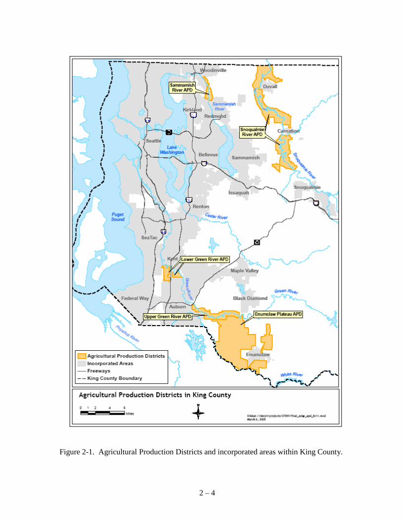
This study was conducted in waterways in or near King County's Agricultural Production

Districts (APDs), which are composed of approximately 40,600 acres (16,430 hectares) zoned

for agricultural use (Figure 2-1). Approximately 483 kilometers (300 miles) of watercourses,

excluding the mainstems (and braids) of the major rivers, flow through King County‟s five APDs

(Lower Green River, Upper Green River, Enumclaw, Sammamish, and Snoqualmie). The APDs

are located almost exclusively on the floodplains of major rivers, with the exception of the

Enumclaw Plateau APD. However, agricultural activities in the Enumclaw Plateau APD occur

on similar extremely flat land, and often affect channels and riparian zones with similar

characteristics to those on the valley floors surrounding large rivers. Sampling for this study

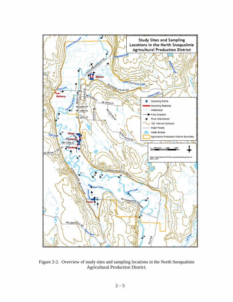
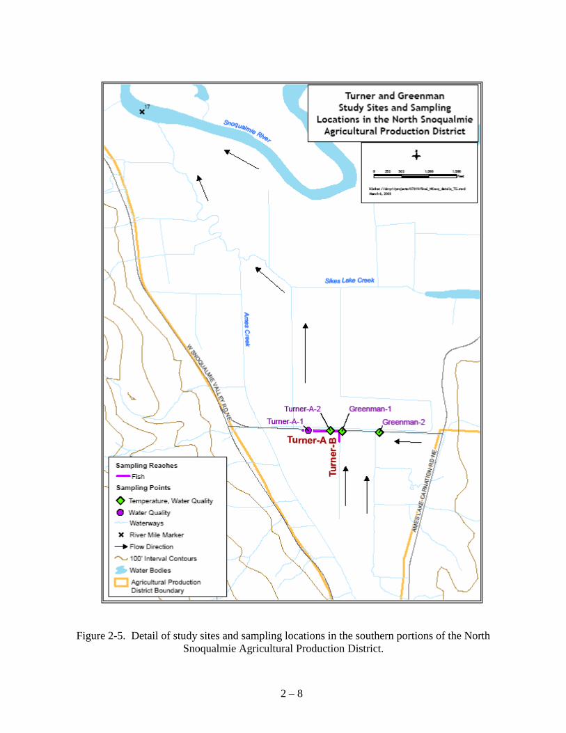
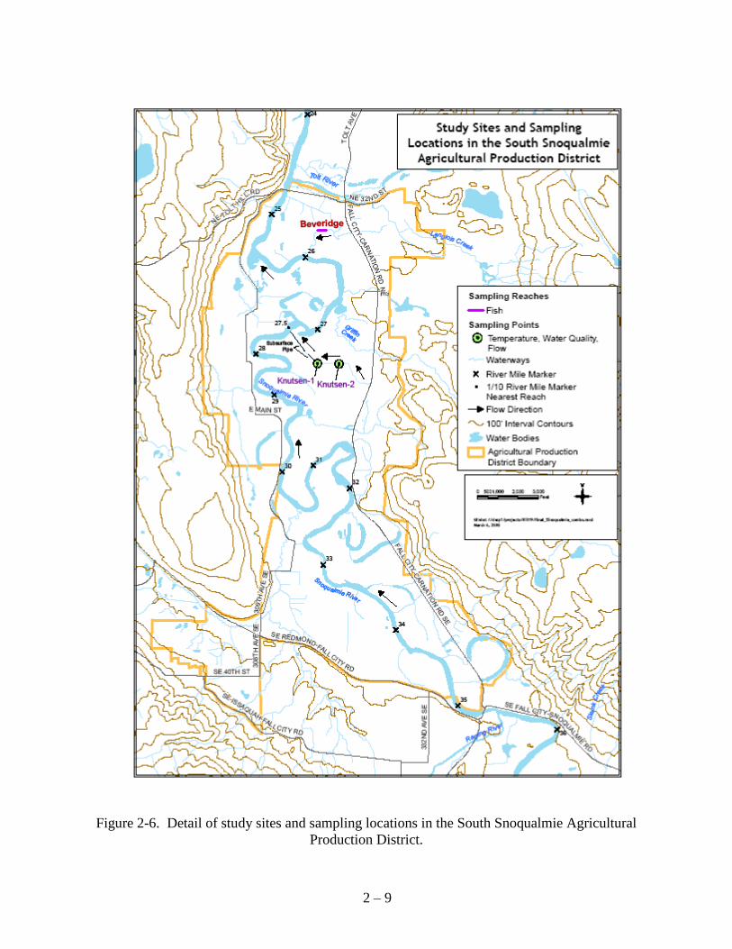
took place in waterways throughout the Snoqualmie (Figure 2-2, Figure 2-3, Figure 2-4, Figure

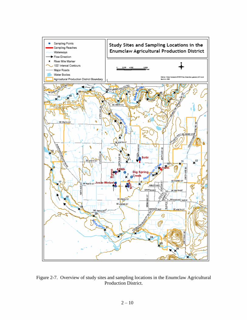
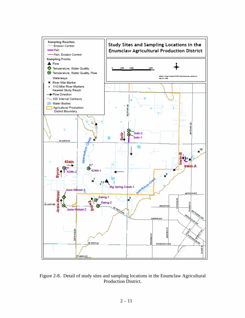
2-5 and Figure 2-6), Enumclaw (Figure 2-7 and Figure 2-8) and Lower Green River (Figure 2-9)

APDs at locations believed to be representative of those found throughout the county‟s five

APDs.

Over time, many floodplain areas within these APDs have become subject to more frequent and

prolonged flooding and as a result extended conditions of saturated soils. Accumulation of fine

sediments and invasive grasses such as reed canarygrass (Phalaris aundinaceae, RCG) in

agricultural drainage networks has added to this dilemma, and leads to repeated flooding. These

recurrent and persistent conditions are of greater concern to agricultural landowners than are

major floods that occasionally inundate extensive valley floor areas. Both the livestock and the

horticultural sectors of the agricultural industry have routinely removed sediment and vegetation

from agricultural watercourses to alleviate chronic flooding of their lands over the last 150 years.

Even crops normally thought of as needing wet soil, such as blueberries, do not thrive in such

highly saturated soils. Yet, the customary method of maintaining watercourses by dredging is

contrary to some of the current fish habitat protection, mitigation, and in some instances

restoration requirements. Anecdotal reports from various areas within King County indicate that

the need for regular maintenance of agricultural drainage channels has increased in recent

decades due to increased runoff from urban and suburban development on the slopes above many

of the farming areas.

In 1979, the voters of King County passed an initiative protecting farmland through the purchase

of development rights. This initiative provided for a bond to establish the King County Farmland

Preservation Program (FPP), which purchases the development rights associated with livestock

and horticultural farmlands to protect them from development. Many of the properties in this

study are enrolled in the FPP. The interest of King County to preserve farmlands within it‟s

boundaries requires development of policies and procedures to facilitate economically viable

agriculture while at the same time complying with requirements of the Endangered Species Act

(ESA). One aim of this study is to enhance the amount of information available regarding use of

agricultural waterways by salmonid listed under the ESA (as well as those not listed) to better

allow farming and fisheries to co-exist on these properties.

http://dnr.metrokc.gov/wlr/lands/farmpp.htm

http://dnr.metrokc.gov/wlr/lands/farmpp.htm

2 – 4

Figure 2-1. Agricultural Production Districts and incorporated areas within King County.

2 – 5

Figure 2-2. Overview of study sites and sampling locations in the North Snoqualmie

Agricultural Production District.

2 – 6

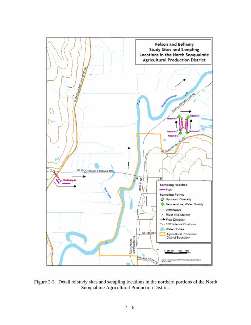
Figure 2-3. Detail of study sites and sampling locations in the northern portions of the North

Snoqualmie Agricultural Production District.

2 – 7

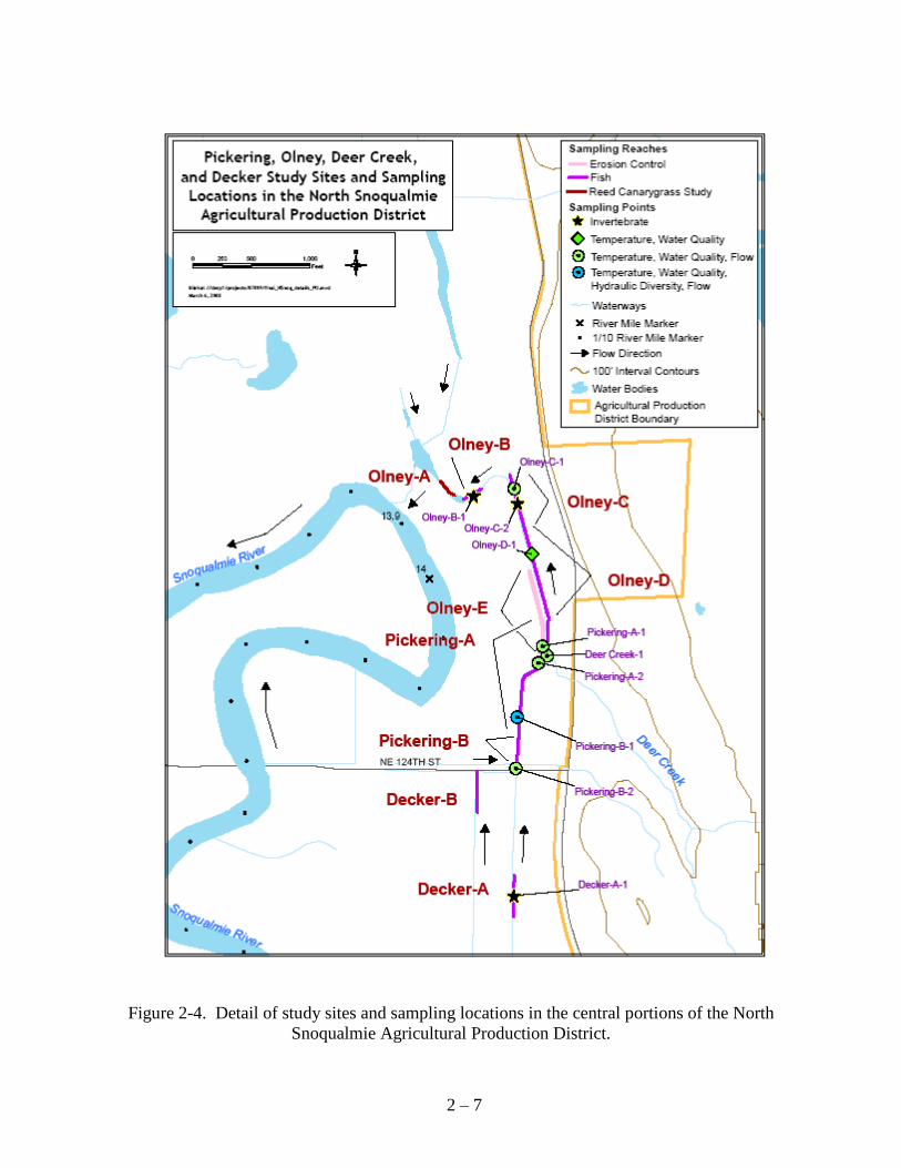
Figure 2-4. Detail of study sites and sampling locations in the central portions of the North


2 – 8

Figure 2-5. Detail of study sites and sampling locations in the southern portions of the North


2 – 9

Figure 2-6. Detail of study sites and sampling locations in the South Snoqualmie Agricultural

Production District.

2 – 10

Figure 2-7. Overview of study sites and sampling locations in the Enumclaw Agricultural


2 – 11

Figure 2-8. Detail of study sites and sampling locations in the Enumclaw Agricultural


2 – 12

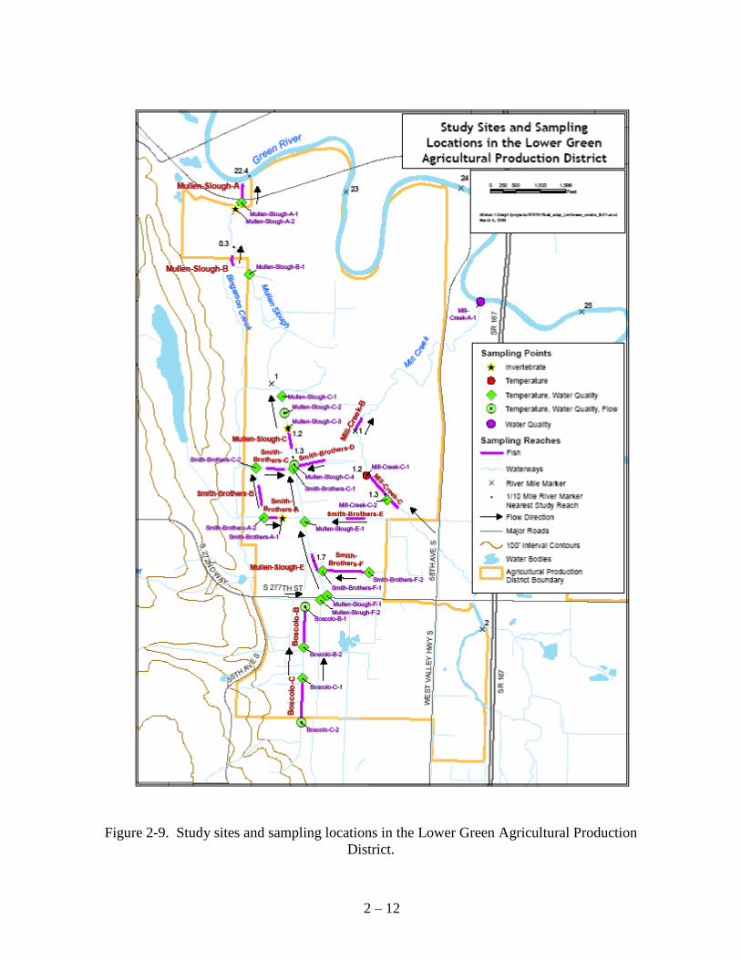
Figure 2-9. Study sites and sampling locations in the Lower Green Agricultural Production

District.

2 – 13

2.3 Methods

2.3.1 Site Selection

Initial site selections were conducted in consultation with King County staff, willing landowners,

and site visits. Vegetative condition and flow source were both considered during site selection.

Vegetative condition was defined by the dominant vegetation surrounding the sampling reach

and was classified as:

1. Reed Canarygrass (RCG).

2. Natural (a mixture of herbaceous vegetation including trees with no or limited RCG

influence).

3. Mixed Vegetation (includes both herbaceous vegetation and a moderate to abundant RCG

influence).

Flow categories were defined as:

1. Natural Flow – Typically found within natural waterway systems (may be channelized)

where flows originate from hillsides, springs, or other natural sources of water.

2. Drainage Flow – Typically found within constructed channels with their origin in the

agricultural area itself (originating from that site or another farm) and conveying

primarily groundwater seepage (including that from drain tiles) and seasonal flood waters

that would otherwise have moved as overland flow.

3. Mixed Flow – A mixture of natural and drainage flow. This is the most common

classification observed within the King County APDs.

Although it was impossible to define and categorize the complete network of all watercourses

throughout the APDs, it is believed that the selected study sites represent a stratified sample of

watercourses with various flow and vegetative conditions represented in proportion to their

occurrence. This assumption is based on examination of existing data and aerial photos,

consultation with KCDNRP staff, and extensive site visits.

2.3.2 Fish Collection

Fish data collected seasonally (January/February, April, July and October) from the fall of 2002

through the spring of 2006 were analyzed for this study component. Fish were collected by

electrofishing according to endangered species protocols defined by the National Marine

Fisheries Service (2000). Fish were anesthetized using MS-222 prior to handling, and allowed to

recover prior to their subsequent release. Length (mm) and wet weight (to nearest 0.5g) were

recorded for the majority of individuals collected. In most cases, length and weight data were

obtained from all fish collected. However, in cases when the numbers of fish collected were

substantial enough to result in fish being retained for extended periods during data recording

(e.g. resulting in undue stress to fish), length and weight information were collected only from a

representative sample of each fish species captured.

2 – 14

Assessment of salmonid origin (hatchery or natural) was made upon the time of capture and

noted on field sheets. Fish origin was determined according to the presence (natural) or absence

(hatchery) of the adipose fin.

2.3.3 Fish Biology

For the most commonly collected salmonid species, definition of life stages was done using

professional judgment of fisheries experts in conjunction with length frequency histograms. For

anadromous coho and Chinook salmon, sub-adult and adult life stages were easily distinguished

from juveniles due to the size of individuals observed. No aging of fish based upon hard body

parts was conducted during this study however, the assigning of ages based on length frequency

histograms is a common alternative to the much more time consuming process of direct aging by

scales or other hard structures (Ney 1993). This methodology allowed for general

characterization of the utilization of agricultural waterways by various juvenile age classes,

however, without age verification using hard structures, this approach did not allow for reliable

statistical analysis of age-specific data.

For rarely collected salmonid species (e.g. chum salmon (O. keta) and rainbow trout (O. mykiss))

assessment of age or life history stages based on length frequency histograms was not possible.

Any discussion of life stages for these species is therefore based solely on professional judgment.

Life history characteristics of coastal cutthroat trout (O. clarki) were not evaluated during this

study. The life history of coastal cutthroat trout may be the most diverse of any Pacific

salmonid, with populations showing great diversity in size and age at maturity as well as a

mixture of anadromous and resident population components (Johnson et al. 1999). Assessment

of life history types and stages of coastal cutthroat trout would have required extensive and

detailed assessment of hard body parts which was not conducted during this study.

Weekly instantaneous growth rate of salmonid species was estimated based on the change in

average length of fish observed between quarterly sampling events and the number of weeks

between sampling events. Since quarterly sampling events typically occurred across a period of

3-4 days, an intermediate sampling date for each event was used in calculation of instantaneous

growth rates. The number of weeks was defined using these intermediate sampling dates and

instantaneous growth rate (G) was estimated as:

t

LLG

)ln()ln( 12 (2.1)

where ln is the symbol for natural logarithm, L1 and L2 are the average length (mm) of fish at

sample time 1 and sample time 2 respectively, and t is the time in weeks between sampling times

1 and 2.

2 – 15

2.3.4 Data Analysis

Collected data included many observations of zero catch which could not be statistically assessed

in conjunction with non-zero catch data. Consequently the data was divided into two subsets

(zero and non-zero data), and processing and data analysis steps were unique for each subset.

Comparison of zero and non-zero catch data across various conditions allowed us to evaluate the

likelihood that salmonids would be found in or associated with various habitat conditions.

Statistical analysis of non-zero catch data allowed us to assess differences in the expected

abundance within habitat conditions where salmonids were found. Similar but separate data

analysis was performed for Chinook salmon, coho salmon, and all salmonids combined. All

statistical analyses were conducted using SAS software (SAS Institute 2006) with a selected

alpha level of 0.10.

Zero and non-zero catch per unit of effort (CPUE) data were summarized across treatment

effects as the percent of observations within each treatment being evaluated (e.g. flow or habitat

category). A chi-square test of homogeneity was conducted to evaluate if zero and non-zero

values were similarly distributed across treatment groups. If the percentage of zero data within

any treatment group was found to be particularly high or low, an avoidance or association

(respectively) with that treatment by salmonids could be inferred.

For non-zero catch data, the CPUE observed at each site during each sampling event (season)

was used for statistical analyses. Doing so removed any effects of variable length of sampling

reaches and/or variable sampling time spent within a given reach. For the purpose of analyses,

100 seconds of shocking time was considered a standard unit of effort.

Analysis of variance (ANOVA) was used to evaluate differences in mean catch rates across

factors or treatments of interest (season, surrounding habitat type, flow type, and distance from

mouth of watercourse system; Table 2-1). Due to the unbalanced design1 of the study, the

General Linear Model procedure (PROC GLM command in SAS) was used to perform all

analysis of variance tests. Evaluation of differences in mean catch rates relied upon test statistics

derived using the Type III sums of squares, also due to the unbalanced nature of the study

design. The ANOVA model evaluated was:

Log (CPUE) = SN + FT + HT + DWM (2.2)

where SN represents season [winter, spring, summer, fall], FT is flow type [natural, drainage,

mixed], HT is habitat type [natural, RCG, mixed], and DWM is the distance from waterway

mouth.

Distance of each site from the mouth of the waterway was not included in the original

contractual study design, but was thought to be potentially important in explaining catch rates

based on professional judgment and observations made during sampling. Distances were

1 The term „unbalanced design‟ refers to the fact that unequal numbers of samples were obtained in the various

treatment groups across sampling events. This is due to a variety of factors such as sites being added or deleted

from the study, high water levels precluding sampling some sites in some seasons, etc. This situation does not

negatively impact the study, but does require additional consideration during data analyses.

2 – 16

estimated using available GIS layers of the drainage networks, and then classified into half-mile

groups (Table 2-1).

Interaction terms (e.g. Season x Habitat) were intentionally excluded from the statistical model.

The high incidence of zero catch data observed during this study, and the resultant need to

separate zero from non-zero catch data for analysis, led to sample sizes being insufficient to

statistically evaluate interaction terms.

The assumption of normality of treatment means was evaluated via a post-ANOVA assessment

using „PROC Univariate Normal‟ commands in SAS. Since only one mean existed for each

treatment, normality of model residuals was examined rather than the raw data. Residuals of

untransformed CPUE data were found to be non-normally distributed (Shapiro Wilk statistic,

p<0.00012). Logarithmic transformation of CPUE data resulted in normalized means for

Chinook salmon, coho salmon and for all salmonids combined (Shapiro Wilk statistic, p>0.6)

and this transformation was therefore used for all analyses of non-zero catch data.

The raw data supporting these analyses are extensive and therefore could not be included with

this document. All data has been supplied to KCDNRP in electronic format.

Table 2-1. Factor levels evaluated for their influence on salmonid catch rates using ANOVA.

Factor Options

Season

Winter (Jan. or Feb.)

Spring (April)

Summer (July)

Fall (October)

Surrounding Habitat Type

Reed Canarygrass (RCG)

Natural Vegetation

Mixed Vegetation

Flow Type

Natural

Drainage

Mixed

Distance Class (from mouth of agricultural waterway)

<0.5 miles

0.5-1.0 miles

1.0-1.5 miles

1.5-2.0 miles

2 Shapiro Wilk statistic tests the hypothesis that the data is normally distributed. If the resultant p-value is small

(e.g. <0.05) the hypothesis is rejected and the data are considered to be non-normally distributed. If the resultant p-

value is relatively large (e.g. >0.25), the hypothesis is not rejected and the data are considered to be normally

distributed. As the p-value increases, so does the relative certainty of data normality.

2 – 17

2.4 Results

2.4.1 Species Characterizations

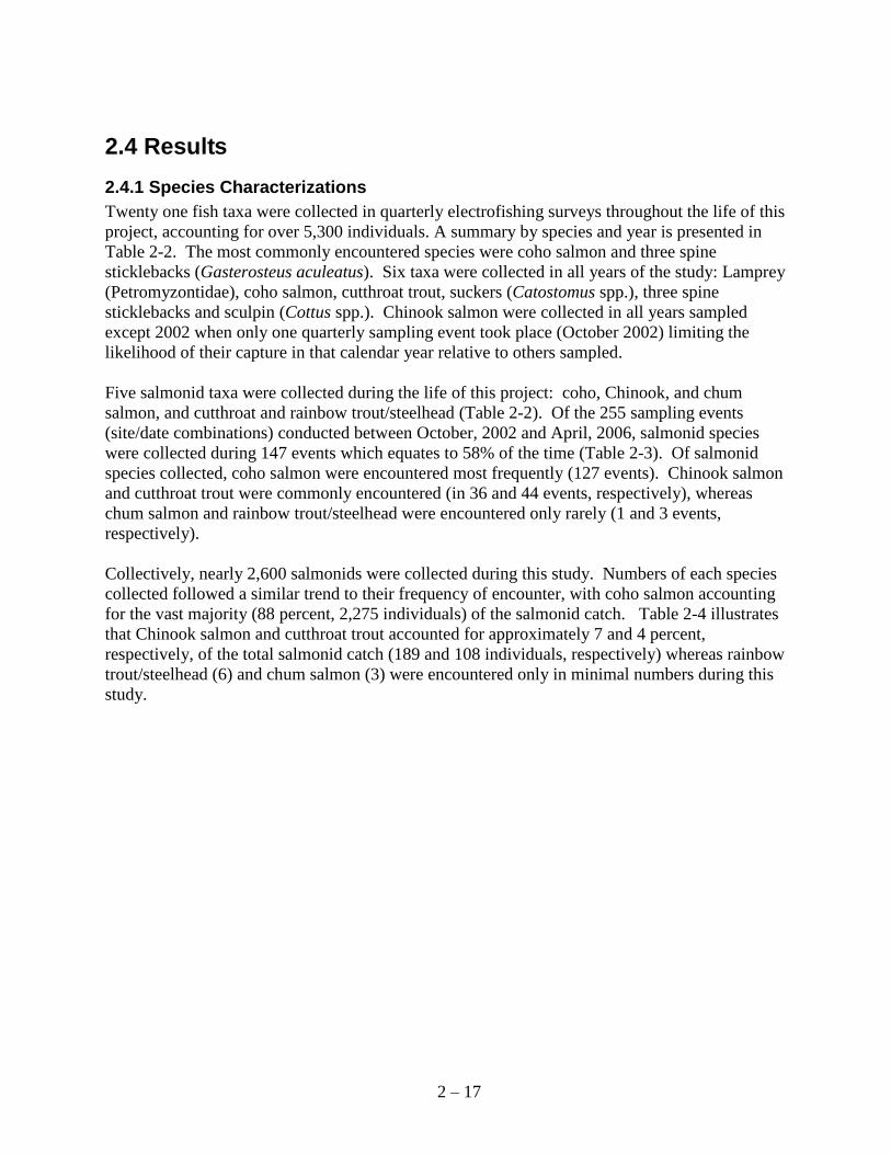
Twenty one fish taxa were collected in quarterly electrofishing surveys throughout the life of this

project, accounting for over 5,300 individuals. A summary by species and year is presented in

Table 2-2. The most commonly encountered species were coho salmon and three spine

sticklebacks (Gasterosteus aculeatus). Six taxa were collected in all years of the study: Lamprey

(Petromyzontidae), coho salmon, cutthroat trout, suckers (Catostomus spp.), three spine

sticklebacks and sculpin (Cottus spp.). Chinook salmon were collected in all years sampled

except 2002 when only one quarterly sampling event took place (October 2002) limiting the

likelihood of their capture in that calendar year relative to others sampled.

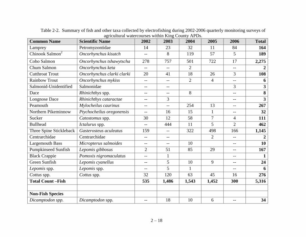
Five salmonid taxa were collected during the life of this project: coho, Chinook, and chum

salmon, and cutthroat and rainbow trout/steelhead (Table 2-2). Of the 255 sampling events

(site/date combinations) conducted between October, 2002 and April, 2006, salmonid species

were collected during 147 events which equates to 58% of the time (Table 2-3). Of salmonid

species collected, coho salmon were encountered most frequently (127 events). Chinook salmon

and cutthroat trout were commonly encountered (in 36 and 44 events, respectively), whereas

chum salmon and rainbow trout/steelhead were encountered only rarely (1 and 3 events,

respectively).

Collectively, nearly 2,600 salmonids were collected during this study. Numbers of each species

collected followed a similar trend to their frequency of encounter, with coho salmon accounting

for the vast majority (88 percent, 2,275 individuals) of the salmonid catch. Table 2-4 illustrates

that Chinook salmon and cutthroat trout accounted for approximately 7 and 4 percent,

respectively, of the total salmonid catch (189 and 108 individuals, respectively) whereas rainbow

trout/steelhead (6) and chum salmon (3) were encountered only in minimal numbers during this

study.

2 – 18

Table 2-2. Summary of fish and other taxa collected by electrofishing during 2002-2006 quarterly monitoring surveys of

agricultural watercourses within King County APDs.

Common Name Scientific Name 2002 2003 2004 2005 2006 Total

Lamprey Petromyzontidae 14 23 32 11 84 164

Chinook Salmon2 Oncorhynchus kisutch -- 8 119 57 5 189

Coho Salmon Oncorhynchus tshawytscha 278 757 501 722 17 2,275

Chum Salmon Oncorhynchus keta -- -- 2 -- 2

Cutthroat Trout Oncorhynchus clarki clarki 20 41 18 26 3 108

Rainbow Trout Oncorhynchus mykiss -- -- 2 4 -- 6

Salmonid-Unidentified Salmonidae -- -- 3 3

Dace Rhinichthys spp. -- -- 8 -- 8

Longnose Dace Rhinichthys cataractae -- 3 -- 3

Peamouth Mylocheilus caurinus -- -- 254 13 -- 267

Northern Pikeminnow Ptychocheilus oregonensis -- 16 15 1 -- 32

Sucker Catostomus spp. 30 12 58 7 4 111

Bullhead Ictalurus spp. -- 444 11 5 2 462

Three Spine Stickleback Gasterosteus aculeatus 159 -- 322 498 166 1,145

Centrarchidae Centrarchidae -- -- 2 -- 2

Largemouth Bass Micropterus salmoides -- -- 10 -- 10

Pumpkinseed Sunfish Lepomis gibbosus 2 51 85 29 -- 167

Black Crappie Pomoxis nigromaculatus -- 1 -- 1

Green Sunfish Lepomis cyanellus -- 5 10 9 -- 24

Lepomis spp. Lepomis spp. -- 5 1 -- 6

Cottus spp. Cottus spp. 32 120 63 45 16 276

Total Count –Fish 535 1,486 1,543 1,452 300 5,316

Non-Fish Species

Dicamptodon spp. Dicamptodon spp. -- 18 10 6 -- 34

2 – 19

Table 2-3. Summary of seasonal fish collections between October, 2002 and April, 2006. Shading represents that sampling occurred;

„S‟ indicate salmonids were collected; „x‟ indicates that only non-salmonid fishes were collected. Site Name APD Vegetative Class Flow Class ‟02 2003 2004 2005 2006

Oct Feb Apr Jul Oct Jan Apr Jul Oct Jan Apr Jul Oct Feb Apr

424th1 Enum Cleaned Mixed -- -- -- -- -- -- -- -- -- -- -- -- S -- --

Byron Enum Natural Mixed -- -- S -- S S x x x -- -- --

Irwin-A Enum Mixed Natural S S S -- -- -- -- -- -- -- -- -- -- -- --

Irwin-B Enum Mixed Drainage S S S S S x S S S S S S -- -- --

Josie-Wetzel2 Enum Cleaned Mix -- -- -- -- -- -- -- -- -- --

Sotir Enum Natural Mixed S S S S x S x S S S S S -- -- --

Boscolo-B3 Lgreen Mixed Mixed x -- -- -- -- -- -- -- -- -- -- -- -- -- --

Boscolo-C3 Lgreen Mixed Mixed x -- -- -- -- -- -- -- -- -- -- -- -- -- --

Mill-Ck-B Lgreen Mixed Natural S -- S S S -- S S -- -- -- -- -- -- --

Mill-Ck-C Lgreen Grass Natural S -- S S S -- S S -- -- -- -- -- -- --

Mullen-Slough-A Lgreen Natural Mixed S S S S S S S S S S S S -- -- --

Mullen-Slough-B Lgreen

Mixed /

Cleaned5 Mixed

x S -- x S S S x S S x

Mullen-Slough-C Lgreen Grass / Cleaned5 Mixed S S S x x x x x x

Mullen-Slough-E Lgreen Grass / Cleaned5 Mixed S x x x x x x x x x

Smith-Bros-A Lgreen

Mixed /

Cleaned5 Natural

S S S x x S S S S S S x x x x

Smith-Bros-B Lgreen Grass / Cleaned5 Natural S S S x x x x x x x x

Smith-Bros-C Lgreen Grass / Cleaned5 Mixed S S S -- -- -- -- -- x x x x

Smith-Bros-E Lgreen Grass / Cleaned5 Drainage x -- -- -- -- -- -- -- --

Smith-Bros-F Lgreen Natural Drainage -- -- -- -- -- -- -- -- -- -- -- -- -- --

Bellamy-C Nsnoq Mixed Mixed -- -- -- -- -- -- -- -- -- -- -- -- S -- --

Bellamy-A Nsnoq Mixed Natural -- -- -- -- -- -- -- -- -- -- -- -- S -- --

Beveridge Nsnoq Grass Natural -- -- -- -- -- -- -- -- -- S S -- -- -- --

Decker-A Nsnoq Mixed Natural S S S S x S S S S S S S S -- x

Decker-B Nsnoq Grass Drainage -- x x x x -- -- --

Nelson-A Nsnoq Grass Drainage -- -- x -- -- S x -- -- -- -- -- -- -- --

Nelson-B Nsnoq Grass Natural -- -- S S S S S S S S S S S -- --

Olney-C Nsnoq Natural Mixed S S S S S S S S S S S S S S S

Olney-D Nsnoq Cleaned Mixed -- -- -- -- -- -- -- -- S S -- S S x S

Pickering5 Nsnoq Grass Mixed S S S x x S S x -- -- -- -- -- -- --

Pickering-A5 Nsnoq Cleaned Mixed -- -- -- -- -- -- -- -- S S S x x S

Pickering-B5 Nsnoq Cleaned Mixed -- -- -- -- -- -- -- -- S S S x S S

Turner A/B Nsnoq Mixed Mixed -- S S S S S S S S S S S -- -- --

2 – 20

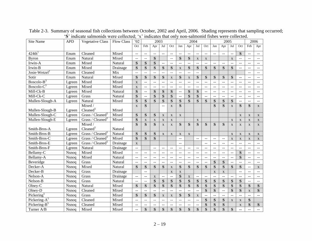
1 Site was surveyed at the request of KCDNRP after maintenance activities occurred. Since no pre-maintenance data was collected at this site, it has been

excluded from data analyses.

2 Site was incorporated at the request of KCDNRP after maintenance activities occurred. Since no fish were collected, it has been excluded from data analyses.

3 Sites on Boscolo property were sampled at the project outset only to validate past findings that salmonids were not present at these sites; All sites have been

excluded from data analyses.

4 Reach had a probable blockage (culvert) at the mouth; following multiple sampling events without fish collection, the site was removed from further study

(including data analyses).

5 Vegetative designations changed following cleaning activities conducted in 2005 between the spring and summer sampling events. At the Pickering site, two

sub-reaches were created following maintenance activities, one of which had LWD installed (Pickering-B) and one of which did not (Pickering-A).

2 – 21

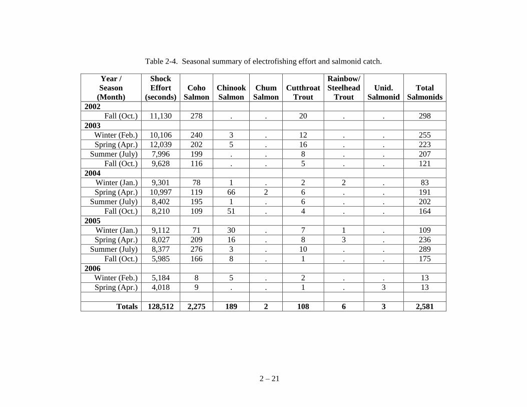
Table 2-4. Seasonal summary of electrofishing effort and salmonid catch.

Year /

Season

(Month)

Shock

Effort

(seconds)

Coho

Salmon

Chinook

Salmon

Chum

Salmon

Cutthroat

Trout

Rainbow/

Steelhead

Trout

Unid.

Salmonid

Total

Salmonids

2002

Fall (Oct.) 11,130 278 . . 20 . . 298

2003

Winter (Feb.) 10,106 240 3 . 12 . . 255

Spring (Apr.) 12,039 202 5 . 16 . . 223

Summer (July) 7,996 199 . . 8 . . 207

Fall (Oct.) 9,628 116 . . 5 . . 121

2004

Winter (Jan.) 9,301 78 1 . 2 2 . 83

Spring (Apr.) 10,997 119 66 2 6 . . 191

Summer (July) 8,402 195 1 . 6 . . 202

Fall (Oct.) 8,210 109 51 . 4 . . 164

2005

Winter (Jan.) 9,112 71 30 . 7 1 . 109

Spring (Apr.) 8,027 209 16 . 8 3 . 236

Summer (July) 8,377 276 3 . 10 . . 289

Fall (Oct.) 5,985 166 8 . 1 . . 175

2006

Winter (Feb.) 5,184 8 5 . 2 . . 13

Spring (Apr.) 4,018 9 . . 1 . 3 13

Totals 128,512 2,275 189 2 108 6 3 2,581

2 – 22

0.00

1.00

2.00

3.00

4.00

Oct.

2002

Feb.

2003

Apr.

2003

July

2003

Oct.

2003

Jan.

2004

Apr.

2004

July

2004

Oct.

2004

Jan.

2005

Apr.

2005

July

2005

Oct.

2005

Feb.

2006

Apr.

2006

Catc

h /

100 s

econds

Coho

Chinook

Cutthroat

Total

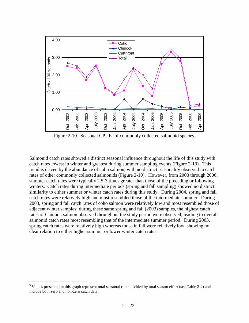
Figure 2-10. Seasonal CPUE

3 of commonly collected salmonid species.

Salmonid catch rates showed a distinct seasonal influence throughout the life of this study with

catch rates lowest in winter and greatest during summer sampling events (Figure 2-10). This

trend is driven by the abundance of coho salmon, with no distinct seasonality observed in catch

rates of other commonly collected salmonids (Figure 2-10). However, from 2003 through 2006,

summer catch rates were typically 2.5-3 times greater than those of the preceding or following

winters. Catch rates during intermediate periods (spring and fall sampling) showed no distinct

similarity to either summer or winter catch rates during this study. During 2004, spring and fall

catch rates were relatively high and most resembled those of the intermediate summer. During

2003, spring and fall catch rates of coho salmon were relatively low and most resembled those of

adjacent winter samples; during these same spring and fall (2003) samples, the highest catch

rates of Chinook salmon observed throughout the study period were observed, leading to overall

salmonid catch rates most resembling that of the intermediate summer period. During 2003,

spring catch rates were relatively high whereas those in fall were relatively low, showing no

clear relation to either higher summer or lower winter catch rates.

3 Values presented in this graph represent total seasonal catch divided by total season effort (see Table 2-4) and

include both zero and non-zero catch data.

2 – 23

2.4.2 Age and Growth of Key Salmonids

2.4.2.1 Coho Salmon

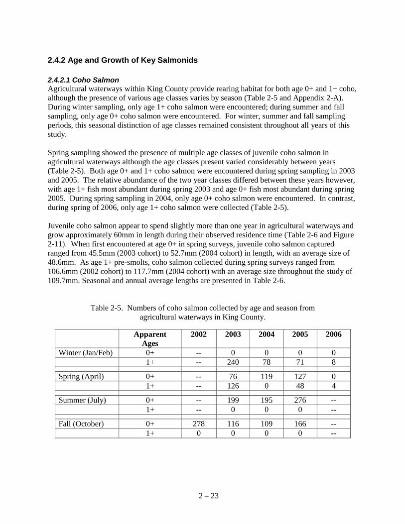
Agricultural waterways within King County provide rearing habitat for both age 0+ and 1+ coho,

although the presence of various age classes varies by season (Table 2-5 and Appendix 2-A).

During winter sampling, only age 1+ coho salmon were encountered; during summer and fall

sampling, only age 0+ coho salmon were encountered. For winter, summer and fall sampling

periods, this seasonal distinction of age classes remained consistent throughout all years of this

study.

Spring sampling showed the presence of multiple age classes of juvenile coho salmon in

agricultural waterways although the age classes present varied considerably between years

(Table 2-5). Both age 0+ and 1+ coho salmon were encountered during spring sampling in 2003

and 2005. The relative abundance of the two year classes differed between these years however,

with age 1+ fish most abundant during spring 2003 and age 0+ fish most abundant during spring

2005. During spring sampling in 2004, only age 0+ coho salmon were encountered. In contrast,

during spring of 2006, only age 1+ coho salmon were collected (Table 2-5).

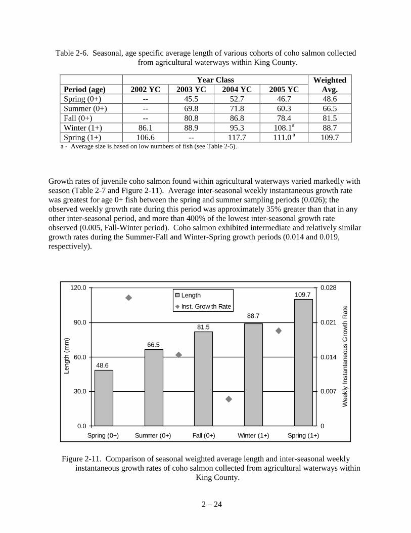
Juvenile coho salmon appear to spend slightly more than one year in agricultural waterways and

grow approximately 60mm in length during their observed residence time (Table 2-6 and Figure

2-11). When first encountered at age 0+ in spring surveys, juvenile coho salmon captured

ranged from 45.5mm (2003 cohort) to 52.7mm (2004 cohort) in length, with an average size of

48.6mm. As age 1+ pre-smolts, coho salmon collected during spring surveys ranged from

106.6mm (2002 cohort) to 117.7mm (2004 cohort) with an average size throughout the study of

109.7mm. Seasonal and annual average lengths are presented in Table 2-6.

Table 2-5. Numbers of coho salmon collected by age and season from

agricultural waterways in King County.

Apparent

Ages

2002 2003 2004 2005 2006

Winter (Jan/Feb) 0+ -- 0 0 0 0

1+ -- 240 78 71 8

Spring (April) 0+ -- 76 119 127 0

1+ -- 126 0 48 4

Summer (July) 0+ -- 199 195 276 --

1+ -- 0 0 0 --

Fall (October) 0+ 278 116 109 166 --

1+ 0 0 0 0 --

2 – 24

Table 2-6. Seasonal, age specific average length of various cohorts of coho salmon collected

from agricultural waterways within King County.

Year Class Weighted

Avg. Period (age) 2002 YC 2003 YC 2004 YC 2005 YC

Spring (0+) -- 45.5 52.7 46.7 48.6

Summer (0+) -- 69.8 71.8 60.3 66.5

Fall (0+) -- 80.8 86.8 78.4 81.5

Winter (1+) 86.1 88.9 95.3 108.1a 88.7

Spring (1+) 106.6 -- 117.7 111.0 a 109.7

a - Average size is based on low numbers of fish (see Table 2-5).

Growth rates of juvenile coho salmon found within agricultural waterways varied markedly with

season (Table 2-7 and Figure 2-11). Average inter-seasonal weekly instantaneous growth rate

was greatest for age 0+ fish between the spring and summer sampling periods (0.026); the

observed weekly growth rate during this period was approximately 35% greater than that in any

other inter-seasonal period, and more than 400% of the lowest inter-seasonal growth rate

observed (0.005, Fall-Winter period). Coho salmon exhibited intermediate and relatively similar

growth rates during the Summer-Fall and Winter-Spring growth periods (0.014 and 0.019,

respectively).

88.7

48.6

66.5

109.7

81.5

0.0

30.0

60.0

90.0

120.0

Spring (0+) Summer (0+) Fall (0+) Winter (1+) Spring (1+)

Length

(m

m)

0

0.007

0.014

0.021

0.028

Weekly

Insta

nta

neous G

row

th R

ate

Length

Inst. Grow th Rate

Figure 2-11. Comparison of seasonal weighted average length and inter-seasonal weekly

instantaneous growth rates of coho salmon collected from agricultural waterways within

King County.

2 – 25

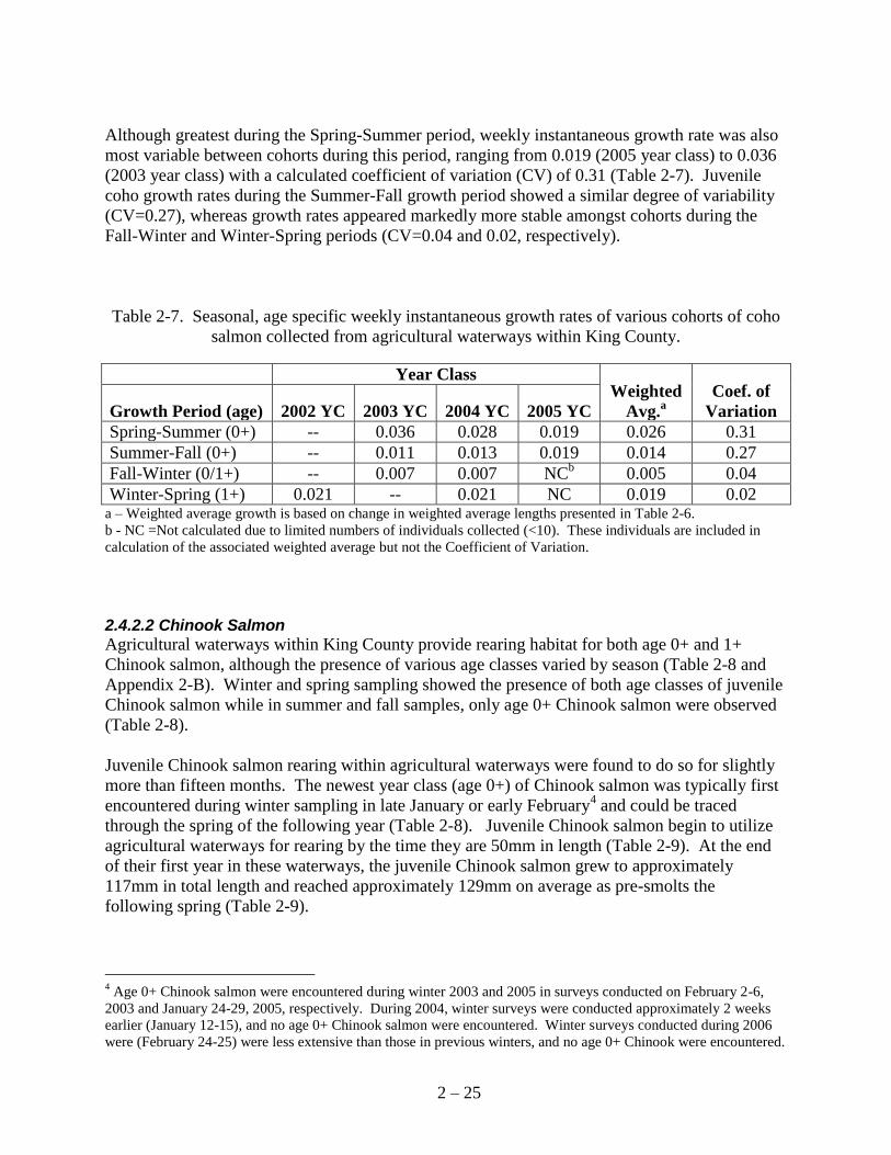
Although greatest during the Spring-Summer period, weekly instantaneous growth rate was also

most variable between cohorts during this period, ranging from 0.019 (2005 year class) to 0.036

(2003 year class) with a calculated coefficient of variation (CV) of 0.31 (Table 2-7). Juvenile

coho growth rates during the Summer-Fall growth period showed a similar degree of variability

(CV=0.27), whereas growth rates appeared markedly more stable amongst cohorts during the

Fall-Winter and Winter-Spring periods (CV=0.04 and 0.02, respectively).

Table 2-7. Seasonal, age specific weekly instantaneous growth rates of various cohorts of coho

salmon collected from agricultural waterways within King County.

Year Class Weighted

Avg.a

Coef. of

Variation Growth Period (age) 2002 YC 2003 YC 2004 YC 2005 YC

Spring-Summer (0+) -- 0.036 0.028 0.019 0.026 0.31

Summer-Fall (0+) -- 0.011 0.013 0.019 0.014 0.27

Fall-Winter (0/1+) -- 0.007 0.007 NCb 0.005 0.04

Winter-Spring (1+) 0.021 -- 0.021 NC 0.019 0.02 a – Weighted average growth is based on change in weighted average lengths presented in Table 2-6.

b - NC =Not calculated due to limited numbers of individuals collected (<10). These individuals are included in

calculation of the associated weighted average but not the Coefficient of Variation.

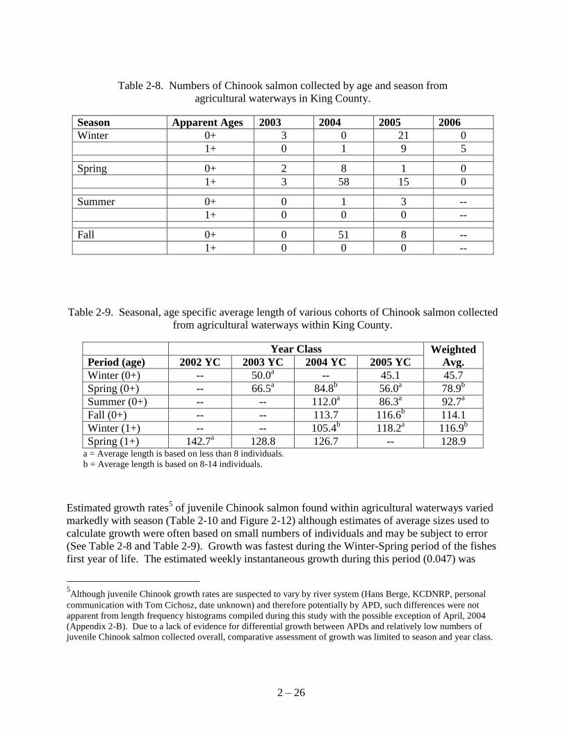
2.4.2.2 Chinook Salmon

Agricultural waterways within King County provide rearing habitat for both age 0+ and 1+

Chinook salmon, although the presence of various age classes varied by season (Table 2-8 and

Appendix 2-B). Winter and spring sampling showed the presence of both age classes of juvenile

Chinook salmon while in summer and fall samples, only age 0+ Chinook salmon were observed

(Table 2-8).

Juvenile Chinook salmon rearing within agricultural waterways were found to do so for slightly

more than fifteen months. The newest year class (age 0+) of Chinook salmon was typically first

encountered during winter sampling in late January or early February4 and could be traced

through the spring of the following year (Table 2-8). Juvenile Chinook salmon begin to utilize

agricultural waterways for rearing by the time they are 50mm in length (Table 2-9). At the end

of their first year in these waterways, the juvenile Chinook salmon grew to approximately

117mm in total length and reached approximately 129mm on average as pre-smolts the

following spring (Table 2-9).

4 Age 0+ Chinook salmon were encountered during winter 2003 and 2005 in surveys conducted on February 2-6,

2003 and January 24-29, 2005, respectively. During 2004, winter surveys were conducted approximately 2 weeks

earlier (January 12-15), and no age 0+ Chinook salmon were encountered. Winter surveys conducted during 2006

were (February 24-25) were less extensive than those in previous winters, and no age 0+ Chinook were encountered.

2 – 26

Table 2-8. Numbers of Chinook salmon collected by age and season from

agricultural waterways in King County.

Season Apparent Ages 2003 2004 2005 2006

Winter 0+ 3 0 21 0

1+ 0 1 9 5

Spring 0+ 2 8 1 0

1+ 3 58 15 0

Summer 0+ 0 1 3 --

1+ 0 0 0 --

Fall 0+ 0 51 8 --

1+ 0 0 0 --

Table 2-9. Seasonal, age specific average length of various cohorts of Chinook salmon collected

from agricultural waterways within King County.

Year Class Weighted

Avg. Period (age) 2002 YC 2003 YC 2004 YC 2005 YC

Winter (0+) -- 50.0a -- 45.1 45.7

Spring (0+) -- 66.5a 84.8

b 56.0

a 78.9

b

Summer (0+) -- -- 112.0a 86.3

a 92.7

a

Fall (0+) -- -- 113.7 116.6b 114.1

Winter (1+) -- -- 105.4b 118.2

a 116.9

b

Spring (1+) 142.7a 128.8 126.7 -- 128.9

a = Average length is based on less than 8 individuals.

b = Average length is based on 8-14 individuals.

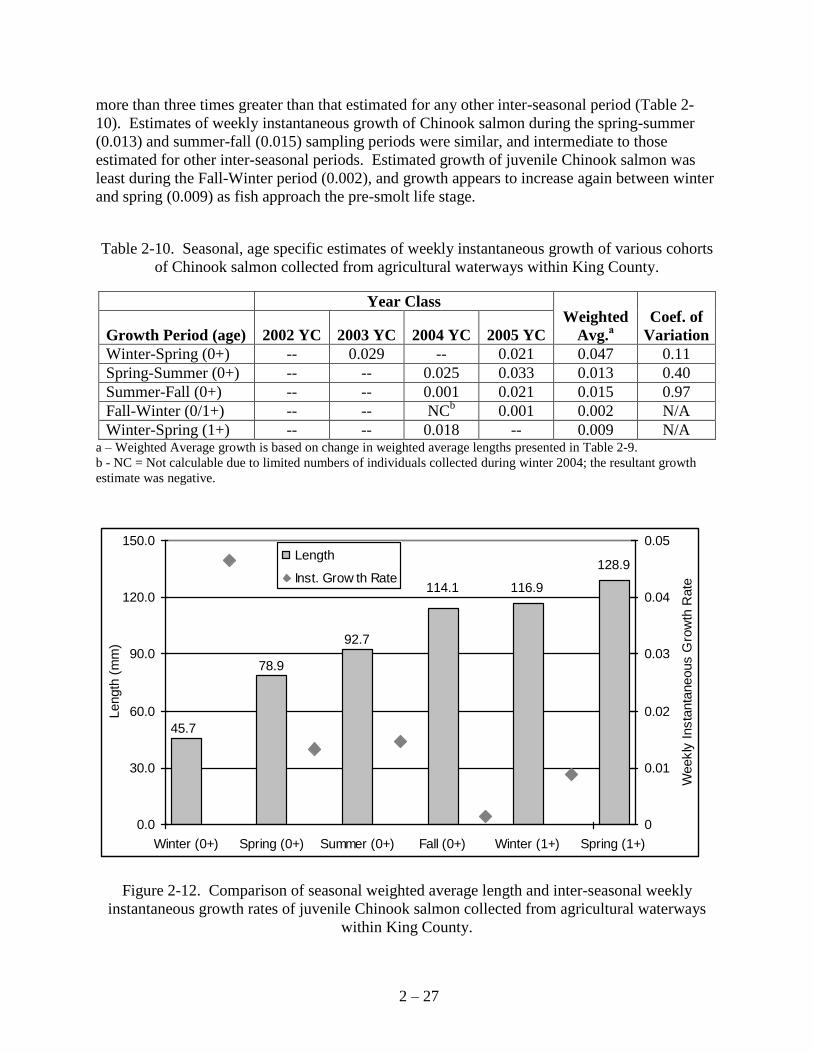
Estimated growth rates5 of juvenile Chinook salmon found within agricultural waterways varied

markedly with season (Table 2-10 and Figure 2-12) although estimates of average sizes used to

calculate growth were often based on small numbers of individuals and may be subject to error

(See Table 2-8 and Table 2-9). Growth was fastest during the Winter-Spring period of the fishes

first year of life. The estimated weekly instantaneous growth during this period (0.047) was

5Although juvenile Chinook growth rates are suspected to vary by river system (Hans Berge, KCDNRP, personal

communication with Tom Cichosz, date unknown) and therefore potentially by APD, such differences were not

apparent from length frequency histograms compiled during this study with the possible exception of April, 2004

(Appendix 2-B). Due to a lack of evidence for differential growth between APDs and relatively low numbers of

juvenile Chinook salmon collected overall, comparative assessment of growth was limited to season and year class.

2 – 27

more than three times greater than that estimated for any other inter-seasonal period (Table 2-

10). Estimates of weekly instantaneous growth of Chinook salmon during the spring-summer

(0.013) and summer-fall (0.015) sampling periods were similar, and intermediate to those

estimated for other inter-seasonal periods. Estimated growth of juvenile Chinook salmon was

least during the Fall-Winter period (0.002), and growth appears to increase again between winter

and spring (0.009) as fish approach the pre-smolt life stage.

Table 2-10. Seasonal, age specific estimates of weekly instantaneous growth of various cohorts

of Chinook salmon collected from agricultural waterways within King County.

Year Class Weighted

Avg.a

Coef. of

Variation Growth Period (age) 2002 YC 2003 YC 2004 YC 2005 YC

Winter-Spring (0+) -- 0.029 -- 0.021 0.047 0.11

Spring-Summer (0+) -- -- 0.025 0.033 0.013 0.40

Summer-Fall (0+) -- -- 0.001 0.021 0.015 0.97

Fall-Winter (0/1+) -- -- NCb 0.001 0.002 N/A

Winter-Spring (1+) -- -- 0.018 -- 0.009 N/A a – Weighted Average growth is based on change in weighted average lengths presented in Table 2-9.

b - NC = Not calculable due to limited numbers of individuals collected during winter 2004; the resultant growth

estimate was negative.

128.9

114.1

92.7

116.9

78.9

45.7

0.0

30.0

60.0

90.0

120.0

150.0

Winter (0+) Spring (0+) Summer (0+) Fall (0+) Winter (1+) Spring (1+)

Length

(m

m)

0

0.01

0.02

0.03

0.04

0.05

Weekly

Insta

nta

neous G

row

th R

ate

Length

Inst. Grow th Rate

Figure 2-12. Comparison of seasonal weighted average length and inter-seasonal weekly

instantaneous growth rates of juvenile Chinook salmon collected from agricultural waterways

within King County.

2 – 28

2.4.3 Temporal, Spatial, and Habitat Distribution of Key Salmonids

2.4.3.1 General Characterization

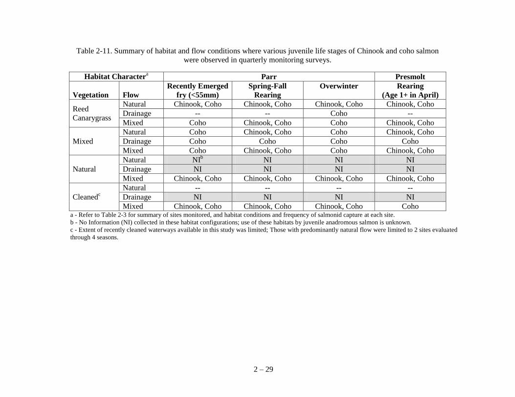
Most habitats available within agricultural waterways are commonly utilized by all juvenile life

history stages of coho salmon. Juvenile coho salmon utilize agricultural waterways as parr

shortly after their emergence from spawning gravels (total length <55mm), as well as for spring,

summer, fall and overwinter rearing (Table 2-11). Coho salmon continued to rear within the

agricultural waterways until shortly before their expected outmigration to the ocean, as

evidenced by their broad distribution across available habitats in the pre-smolt stage as age 1+

fish collected during spring monitoring.

Illustrating the importance of agricultural waterways to juvenile coho salmon, all juvenile life

stages were collected from each of the habitat configurations evaluated with only two exceptions

(Table 2-11). Juvenile coho salmon were not found in a limited sample6 of recently cleaned (of

vegetation) waterways with predominantly natural flows. Additionally, juvenile coho salmon

were found to utilize waterways with predominantly RCG vegetation coupled with drainage

flows only on a single occasion in which a number of individuals (14) were found overwintering

in a waterway with those conditions (Nelson-A, January 2004; refer to Table 2-3).

Juvenile Chinook salmon utilize agricultural waterways as parr shortly after their emergence

from spawning gravels (total length <55mm), as well as for spring, summer, fall and overwinter

rearing (Table 2-11). Most habitats available within agricultural waterways were utilized by 2-3

juvenile life history stages of Chinook salmon, although few habitat conditions had observed

utilization by all four life history stages evaluated. Recently emergent and overwintering

juveniles however were observed in fewer habitat configurations than those rearing from spring

through fall or as age 1+ pre-smolts.

No juvenile Chinook salmon were collected from waterways dominated by drainage flows

during this study (Table 2-11). In RCG dominated vegetation, more life history stages of

juvenile Chinook salmon were found in waterways dominated by natural flows (all four life

stages) than those dominated by mixed flow conditions (spring-fall and pre-smolt rearing only).

The same was not true of mixed vegetation sites in which both mixed and natural flow conditions

had only spring-fall rearing (including pre-smolt rearing). Under a natural vegetative regime

only mixed flow conditions were evaluated and all juvenile life history stages of Chinook salmon

were encountered under these conditions. In waterways with banks/channels recently cleaned of

vegetation, juvenile Chinook salmon were not encountered during limited sampling; more

extensive sampling was conducted in recently cleaned waterways with mixed flow conditions

and juvenile Chinook salmon were collected as recent emergent fry and during spring, summer,

fall and overwinter rearing stages.

6 Evaluation of this habitat configuration involved only two sites (Smith-Bros-A and Smith-Bros-B) located on

adjacent and connected waterways. Each site was sampled during 4 seasonal sampling events following cleaning of

vegetation from the channels.

2 – 29

Table 2-11. Summary of habitat and flow conditions where various juvenile life stages of Chinook and coho salmon

were observed in quarterly monitoring surveys.

Habitat Charactera Parr Presmolt

Vegetation Flow

Recently Emerged

fry (<55mm)

Spring-Fall

Rearing

Overwinter Rearing

(Age 1+ in April)

Reed

Canarygrass

Natural Chinook, Coho Chinook, Coho Chinook, Coho Chinook, Coho

Drainage -- -- Coho --

Mixed Coho Chinook, Coho Coho Chinook, Coho

Mixed

Natural Coho Chinook, Coho Coho Chinook, Coho

Drainage Coho Coho Coho Coho

Mixed Coho Chinook, Coho Coho Chinook, Coho

Natural

Natural NIb NI NI NI

Drainage NI NI NI NI

Mixed Chinook, Coho Chinook, Coho Chinook, Coho Chinook, Coho

Cleanedc

Natural -- -- -- --

Drainage NI NI NI NI

Mixed Chinook, Coho Chinook, Coho Chinook, Coho Coho a - Refer to Table 2-3 for summary of sites monitored, and habitat conditions and frequency of salmonid capture at each site.

b - No Information (NI) collected in these habitat configurations; use of these habitats by juvenile anadromous salmon is unknown.

c - Extent of recently cleaned waterways available in this study was limited; Those with predominantly natural flow were limited to 2 sites evaluated

through 4 seasons.

2 – 30

2.4.3.2 Statistical Characterization

Zero Versus Non-Zero Catch Data

Salmonids, as indicated by total catch, were encountered in all seasons, distance classes, and

habitat and flow conditions evaluated during this study. However, differences in their likelihood

of encounter were observed across all of these factors. Moreover, the distribution of non-zero

catch data differed significantly from that of zero catch data across season, distance class,

vegetative habitat type and flow type (Chi square test, p<0.10; Figure 2-13). Chi square

evaluation allows for evaluation of differences in distributions across all classes of a variable

(e.g. season or habitat type) but does not allow for pairwise comparisons within classes (e.g. zero

versus non-zero catch during summer). Consequently, interpretation of intra-class differences is

subjective.

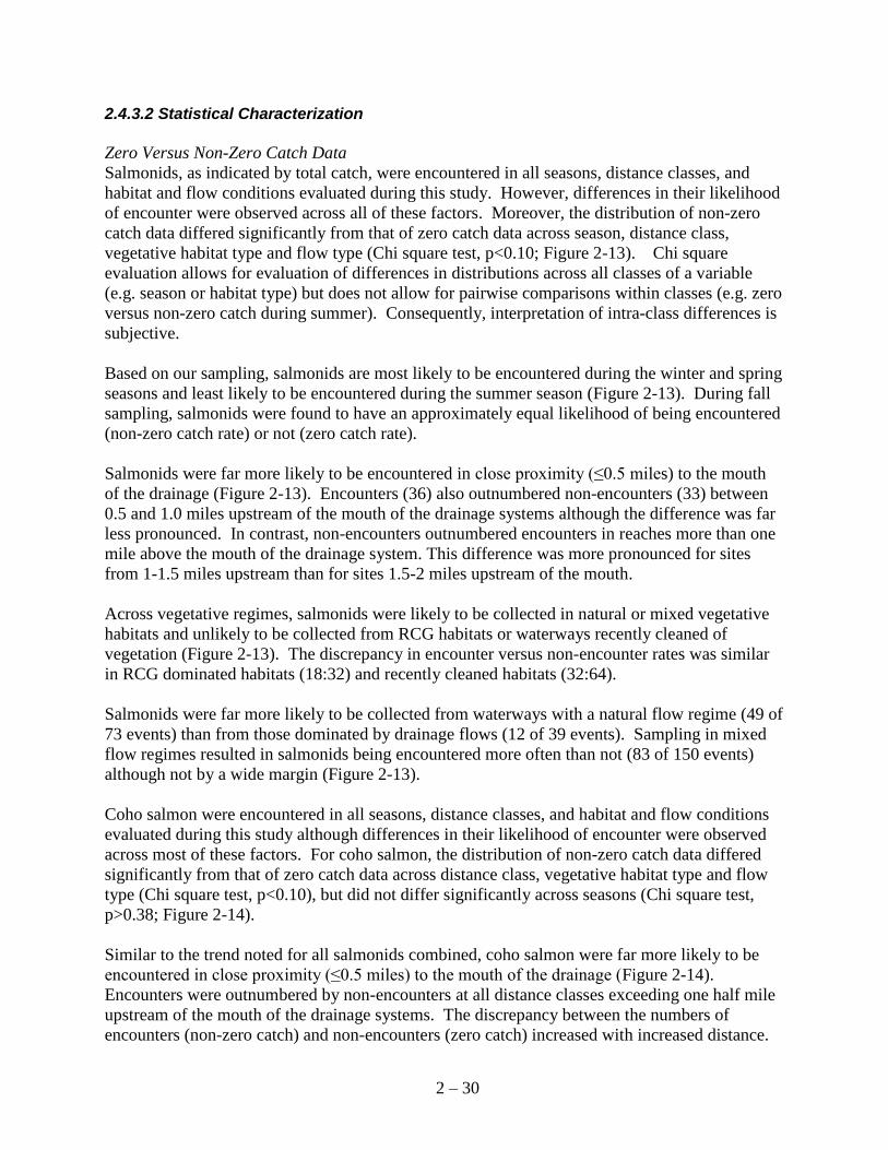
Based on our sampling, salmonids are most likely to be encountered during the winter and spring

seasons and least likely to be encountered during the summer season (Figure 2-13). During fall

sampling, salmonids were found to have an approximately equal likelihood of being encountered

(non-zero catch rate) or not (zero catch rate).

Salmonids were far more likely to be encountered in close proximity (≤0.5 miles) to the mouth

of the drainage (Figure 2-13). Encounters (36) also outnumbered non-encounters (33) between

0.5 and 1.0 miles upstream of the mouth of the drainage systems although the difference was far

less pronounced. In contrast, non-encounters outnumbered encounters in reaches more than one

mile above the mouth of the drainage system. This difference was more pronounced for sites

from 1-1.5 miles upstream than for sites 1.5-2 miles upstream of the mouth.

Across vegetative regimes, salmonids were likely to be collected in natural or mixed vegetative

habitats and unlikely to be collected from RCG habitats or waterways recently cleaned of

vegetation (Figure 2-13). The discrepancy in encounter versus non-encounter rates was similar

in RCG dominated habitats (18:32) and recently cleaned habitats (32:64).

Salmonids were far more likely to be collected from waterways with a natural flow regime (49 of

73 events) than from those dominated by drainage flows (12 of 39 events). Sampling in mixed

flow regimes resulted in salmonids being encountered more often than not (83 of 150 events)

although not by a wide margin (Figure 2-13).

Coho salmon were encountered in all seasons, distance classes, and habitat and flow conditions

evaluated during this study although differences in their likelihood of encounter were observed

across most of these factors. For coho salmon, the distribution of non-zero catch data differed

significantly from that of zero catch data across distance class, vegetative habitat type and flow

type (Chi square test, p<0.10), but did not differ significantly across seasons (Chi square test,

p>0.38; Figure 2-14).

Similar to the trend noted for all salmonids combined, coho salmon were far more likely to be

encountered in close proximity (≤0.5 miles) to the mouth of the drainage (Figure 2-14).

Encounters were outnumbered by non-encounters at all distance classes exceeding one half mile

upstream of the mouth of the drainage systems. The discrepancy between the numbers of

encounters (non-zero catch) and non-encounters (zero catch) increased with increased distance.

2 – 31

Count By Season

0

10

20

30

40

50

60

70

80

90

Winter Spring Summer Fall

Zero

Non-zero

Count By Distance

0

10

20

30

40

50

60

70

80

90

0-0.5 mile 0.5-1 mile 1-1.5 mile 1.5-2 mile

Zero

Non-zero

Count By Habitat Type

0

10

20

30

40

50

60

70

80

90

Cleaned Grass Mixed Natural

Zero

Non-zero

Count By Flow Type

0

10

20

30

40

50

60

70

80

90

Drainage Mixed Natural

Zero

Non-zero

Figure 2-13. Count of total salmonid zero and non-zero catch observations by season, distance,

habitat, and flow type.

Chi Square p=0.0011

Chi Square p<0.0001

Chi Square p=0.0627

Chi Square p<0.0001

2 – 32

Count by Season

0

10

20

30

40

50

60

70

80


Zero

Non-zero

Count by Distance

0

10

20

30

40

50

60

70

80


Zero

Non-zero

Count by Habitat Type

0

10

20

30

40

50

60

70

80


Zero

Non-zero

Count by Flow Type

0

10

20

30

40

50

60

70

80


Zero

Non-zero

Figure 2-14. Count of coho salmon zero and non-zero catch observations by season, distance,

habitat, and flow type.

Chi Square p=0.0001

Chi Square p=.3844

Chi Square p<0.0001

Chi Square p=0.0520

2 – 33

Coho salmon were very likely to be collected in natural or mixed vegetative habitats and unlikely

to be collected from RCG habitats or waterways recently cleaned of vegetation (Figure 2-14).

This is similar to the trend noted for all salmonids combined.

With respect to flow type, coho salmon were least likely to be collected from waterways

dominated by drainage flow, where the number of non-encounters (27) outnumbered encounters

(12) substantially (Figure 2-14). In channels with predominantly mixed flow, coho salmon were

encountered less often than not (71 of 150 events) although by only a narrow margin. Natural

flow was the only flow condition in which coho salmon encounters (40) outnumbered non-

encounters (33) although this did not appear to be a substantial difference.

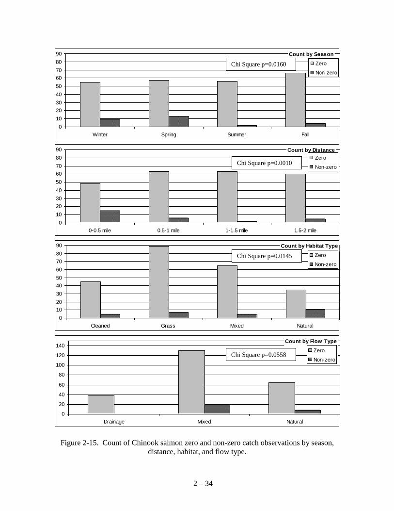
Chinook salmon were encountered in all seasons, distance classes, and habitat conditions

evaluated during this study; they were encountered from only two of three flow regimes sampled

during this study (mixed and natural, not drainage flow; Figure 2-15). Chinook salmon zero and

non-zero catch distributions varied significantly across season, distance class, vegetative habitat

type and flow type (Chi square test, p<0.10; Figure 2-15). In general, Chinook salmon were less

likely to be encountered than either coho salmon or salmonids (as evidenced by lower number of

non-zero catch observations) across all seasons, distance classes and habitat or flow regimes

(Figure 2-15, Figure 2-13 and Figure 2-14, respectively).

Although uncommonly collected throughout the study, Chinook salmon were most frequently

encountered during spring and winter samples, and least frequently encountered during summer

sampling (Figure 2-15). Chinook salmon were most commonly encountered in reaches nearer

the mouth of the drainage system in which they were located, and appeared to exhibit an affinity

for natural vegetative habitats and an avoidance of RCG dominated habitats. Chinook salmon

were not collected from waterways dominated by drainage flows, and showed no apparent

affinity nor avoidance of those sites dominated by either mixed or natural flow regimes. These

patterns are similar to those observed for both coho salmon and total salmonid catch statistics.

2 – 34

Count by Season

0

10

20

30

40

50

60

70

80

90


Zero

Non-zero

Count by Distance

0

10

20

30

40

50

60

70

80

90


Zero

Non-zero

Count by Habitat Type

0

10

20

30

40

50

60

70

80

90


Zero

Non-zero

Count by Flow Type

0

20

40

60

80

100

120

140


Zero

Non-zero

Figure 2-15. Count of Chinook salmon zero and non-zero catch observations by season,

distance, habitat, and flow type.

Chi Square p=0.0558

Chi Square p=0.0010

Chi Square p=0.0145

Chi Square p=0.0160

2 – 35

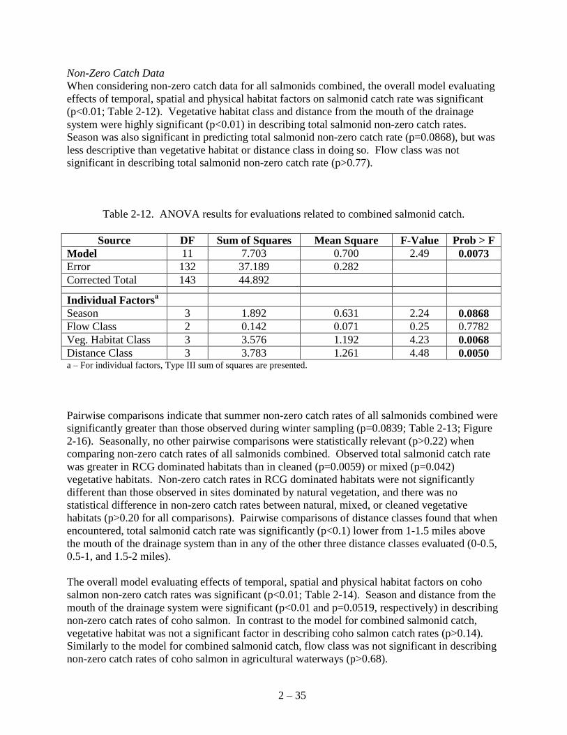
Non-Zero Catch Data

When considering non-zero catch data for all salmonids combined, the overall model evaluating

effects of temporal, spatial and physical habitat factors on salmonid catch rate was significant

(p<0.01; Table 2-12). Vegetative habitat class and distance from the mouth of the drainage

system were highly significant (p<0.01) in describing total salmonid non-zero catch rates.

Season was also significant in predicting total salmonid non-zero catch rate (p=0.0868), but was

less descriptive than vegetative habitat or distance class in doing so. Flow class was not

significant in describing total salmonid non-zero catch rate (p>0.77).

Table 2-12. ANOVA results for evaluations related to combined salmonid catch.

Source DF Sum of Squares Mean Square F-Value Prob > F

Model 11 7.703 0.700 2.49 0.0073

Error 132 37.189 0.282

Corrected Total 143 44.892

Individual Factors

a

Season 3 1.892 0.631 2.24 0.0868

Flow Class 2 0.142 0.071 0.25 0.7782

Veg. Habitat Class 3 3.576 1.192 4.23 0.0068

Distance Class 3 3.783 1.261 4.48 0.0050 a – For individual factors, Type III sum of squares are presented.

Pairwise comparisons indicate that summer non-zero catch rates of all salmonids combined were

significantly greater than those observed during winter sampling (p=0.0839; Table 2-13; Figure

2-16). Seasonally, no other pairwise comparisons were statistically relevant (p>0.22) when

comparing non-zero catch rates of all salmonids combined. Observed total salmonid catch rate

was greater in RCG dominated habitats than in cleaned (p=0.0059) or mixed (p=0.042)

vegetative habitats. Non-zero catch rates in RCG dominated habitats were not significantly

different than those observed in sites dominated by natural vegetation, and there was no

statistical difference in non-zero catch rates between natural, mixed, or cleaned vegetative

habitats (p>0.20 for all comparisons). Pairwise comparisons of distance classes found that when

encountered, total salmonid catch rate was significantly (p<0.1) lower from 1-1.5 miles above

the mouth of the drainage system than in any of the other three distance classes evaluated (0-0.5,

0.5-1, and 1.5-2 miles).

The overall model evaluating effects of temporal, spatial and physical habitat factors on coho

salmon non-zero catch rates was significant (p<0.01; Table 2-14). Season and distance from the

mouth of the drainage system were significant (p<0.01 and p=0.0519, respectively) in describing

non-zero catch rates of coho salmon. In contrast to the model for combined salmonid catch,

vegetative habitat was not a significant factor in describing coho salmon catch rates (p>0.14).

Similarly to the model for combined salmonid catch, flow class was not significant in describing

non-zero catch rates of coho salmon in agricultural waterways (p>0.68).

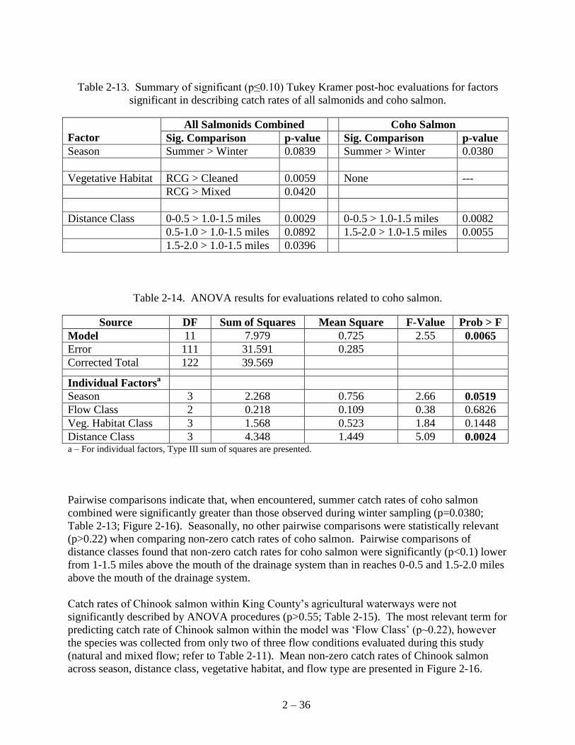
2 – 36

Table 2-13. Summary of significant (p≤0.10) Tukey Kramer post-hoc evaluations for factors

significant in describing catch rates of all salmonids and coho salmon.

Factor

All Salmonids Combined Coho Salmon

Sig. Comparison p-value Sig. Comparison p-value

Season Summer > Winter 0.0839 Summer > Winter 0.0380

Vegetative Habitat RCG > Cleaned 0.0059 None ---

RCG > Mixed 0.0420

Distance Class 0-0.5 > 1.0-1.5 miles 0.0029 0-0.5 > 1.0-1.5 miles 0.0082

0.5-1.0 > 1.0-1.5 miles 0.0892 1.5-2.0 > 1.0-1.5 miles 0.0055

1.5-2.0 > 1.0-1.5 miles 0.0396

Table 2-14. ANOVA results for evaluations related to coho salmon.


Model 11 7.979 0.725 2.55 0.0065

Error 111 31.591 0.285


Individual Factors

a

Season 3 2.268 0.756 2.66 0.0519

Flow Class 2 0.218 0.109 0.38 0.6826



Pairwise comparisons indicate that, when encountered, summer catch rates of coho salmon

combined were significantly greater than those observed during winter sampling (p=0.0380;

Table 2-13; Figure 2-16). Seasonally, no other pairwise comparisons were statistically relevant

(p>0.22) when comparing non-zero catch rates of coho salmon. Pairwise comparisons of

distance classes found that non-zero catch rates for coho salmon were significantly (p<0.1) lower

from 1-1.5 miles above the mouth of the drainage system than in reaches 0-0.5 and 1.5-2.0 miles

above the mouth of the drainage system.

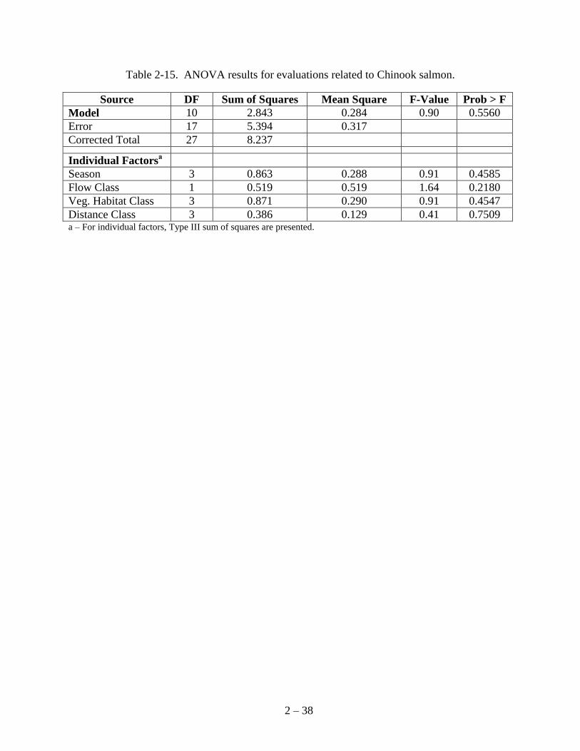
Catch rates of Chinook salmon within King County‟s agricultural waterways were not

significantly described by ANOVA procedures (p>0.55; Table 2-15). The most relevant term for

predicting catch rate of Chinook salmon within the model was „Flow Class‟ (p~0.22), however

the species was collected from only two of three flow conditions evaluated during this study

(natural and mixed flow; refer to Table 2-11). Mean non-zero catch rates of Chinook salmon

across season, distance class, vegetative habitat, and flow type are presented in Figure 2-16.

2 – 37

By Season

0

2

4

6

8

10

12

14

16


Fis

h/1

00 s

econds

Total Salmonid CPUE

Coho Salmon CPUE

Chinook Salmon CPUE

By Distance

0

2

4

6

8

10

12

14

16


Fis

h/1

00 s

econds

Total Salmonid CPUE

Coho Salmon CPUE

Chinook Salmon CPUE

By Habitat

0

2

4

6

8

10

12

14

16


Fis

h/1

00 s

econds

Total Salmonid CPUE

Coho Salmon CPUE

Chinook Salmon CPUE

By Flow

0

2

4

6

8

10

12

14

16


Fis

h/1

00 s

econds

Total Salmonid CPUE

Coho Salmon CPUE

Chinook Salmon CPUE

Figure 2-16. Depiction of mean non-zero CPUE for combined salmonids, coho salmon and Chinook salmon across seasons, distance

classes, vegetative habitats and flow classes. Error bars are ± one standard deviation.

2 – 38

Table 2-15. ANOVA results for evaluations related to Chinook salmon.


Model 10 2.843 0.284 0.90 0.5560

Error 17 5.394 0.317


Individual Factors

a

Season 3 0.863 0.288 0.91 0.4585

Flow Class 1 0.519 0.519 1.64 0.2180



2 – 39

2.5 Discussion

2.5.1 Life History Characteristics

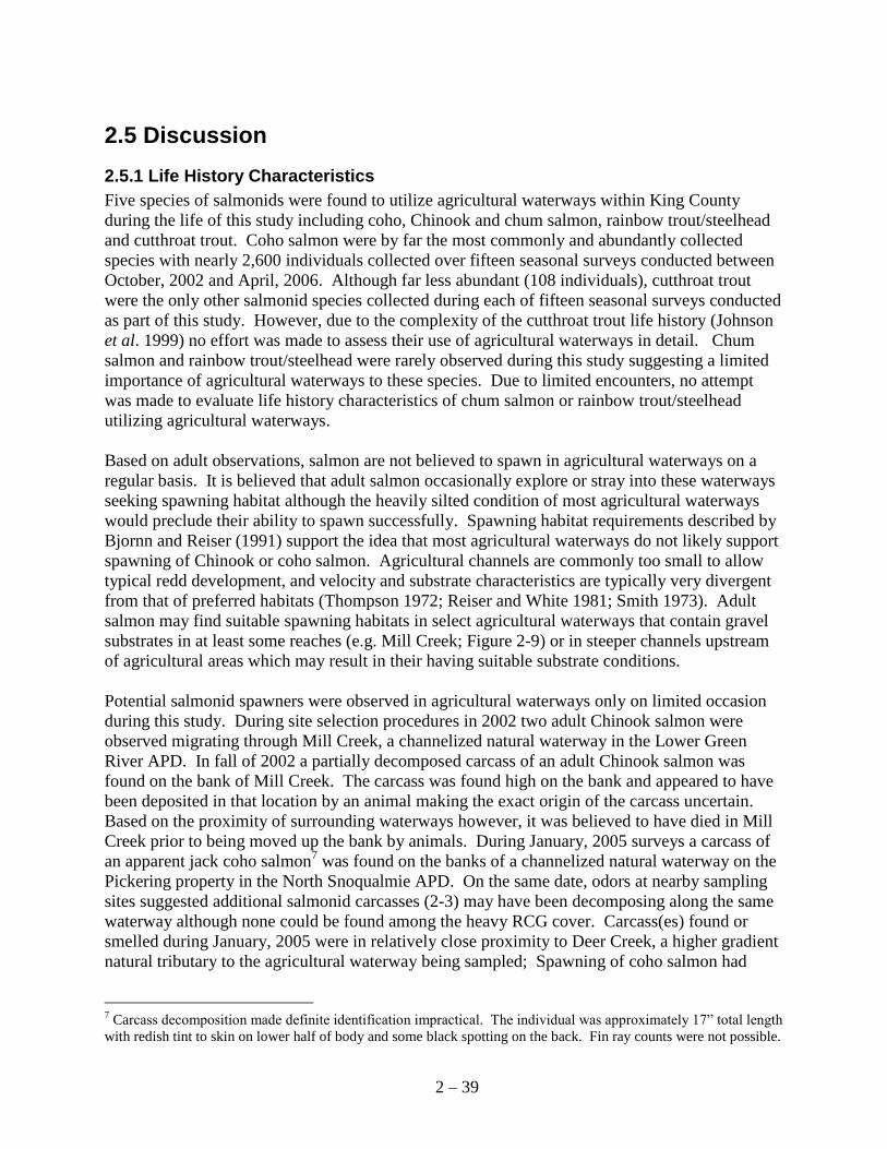
Five species of salmonids were found to utilize agricultural waterways within King County

during the life of this study including coho, Chinook and chum salmon, rainbow trout/steelhead

and cutthroat trout. Coho salmon were by far the most commonly and abundantly collected

species with nearly 2,600 individuals collected over fifteen seasonal surveys conducted between

October, 2002 and April, 2006. Although far less abundant (108 individuals), cutthroat trout

were the only other salmonid species collected during each of fifteen seasonal surveys conducted

as part of this study. However, due to the complexity of the cutthroat trout life history (Johnson

et al. 1999) no effort was made to assess their use of agricultural waterways in detail. Chum

salmon and rainbow trout/steelhead were rarely observed during this study suggesting a limited

importance of agricultural waterways to these species. Due to limited encounters, no attempt

was made to evaluate life history characteristics of chum salmon or rainbow trout/steelhead

utilizing agricultural waterways.

Based on adult observations, salmon are not believed to spawn in agricultural waterways on a

regular basis. It is believed that adult salmon occasionally explore or stray into these waterways

seeking spawning habitat although the heavily silted condition of most agricultural waterways

would preclude their ability to spawn successfully. Spawning habitat requirements described by

Bjornn and Reiser (1991) support the idea that most agricultural waterways do not likely support

spawning of Chinook or coho salmon. Agricultural channels are commonly too small to allow

typical redd development, and velocity and substrate characteristics are typically very divergent

from that of preferred habitats (Thompson 1972; Reiser and White 1981; Smith 1973). Adult

salmon may find suitable spawning habitats in select agricultural waterways that contain gravel

substrates in at least some reaches (e.g. Mill Creek; Figure 2-9) or in steeper channels upstream

of agricultural areas which may result in their having suitable substrate conditions.

Potential salmonid spawners were observed in agricultural waterways only on limited occasion

during this study. During site selection procedures in 2002 two adult Chinook salmon were

observed migrating through Mill Creek, a channelized natural waterway in the Lower Green

River APD. In fall of 2002 a partially decomposed carcass of an adult Chinook salmon was

found on the bank of Mill Creek. The carcass was found high on the bank and appeared to have

been deposited in that location by an animal making the exact origin of the carcass uncertain.

Based on the proximity of surrounding waterways however, it was believed to have died in Mill

Creek prior to being moved up the bank by animals. During January, 2005 surveys a carcass of

an apparent jack coho salmon7 was found on the banks of a channelized natural waterway on the

Pickering property in the North Snoqualmie APD. On the same date, odors at nearby sampling

sites suggested additional salmonid carcasses (2-3) may have been decomposing along the same

waterway although none could be found among the heavy RCG cover. Carcass(es) found or

smelled during January, 2005 were in relatively close proximity to Deer Creek, a higher gradient

natural tributary to the agricultural waterway being sampled; Spawning of coho salmon had

7 Carcass decomposition made definite identification impractical. The individual was approximately 17” total length

with redish tint to skin on lower half of body and some black spotting on the back. Fin ray counts were not possible.

2 – 40

previously been observed in Deer Creek (Hans Berge, KCDNRP personal communication with

Tom Cichosz, February 2005).

It is important to note that cutthroat trout have very different spawning requirements than salmon

with regard to preferred depth, velocity and substrate size (Bjornn and Reiser 1991). These

differences suggest that regular or relatively widespread spawning of cutthroat trout is more

likely than that of other salmonid species in agricultural waterways. However, observations of

habitat conditions during this study (particularly the heavy siltation of channels and lack of

underlying gravel in most cases) suggest that suitable spawning areas for cutthroat trout are also

likely limited to select reaches in agricultural waterways and/or steeper channels upstream of

agricultural areas which have higher velocity and presence of suitable spawning substrates.

Cutthroat trout were commonly collected during this study and found to be relatively widely

distributed in agricultural waterways. The fact that the species was commonly collected and

widely distributed illustrates that agricultural waterways do provide important habitats for

cutthroat trout. However, due to relatively limited numbers collected, detailed evaluation of their

use of agricultural waterways was impractical.

Of species and life stages closely evaluated during this study, agricultural waterways within King

County are most important to juvenile coho and Chinook salmon. Agricultural waterways

provide important habitat for rearing of age 0+ and 1+ Chinook and coho salmon and are utilized

by both species throughout their juvenile life histories from shortly after emergence to the pre-

smolt stage prior to their outmigration to salt water. Juvenile coho and Chinook salmon were

both encountered in all four seasons monitored, and multiple age classes (0+ and 1+) of both

species were encountered.

Our findings indicate that Chinook salmon enter the agricultural waterways at age 0+ earlier (late

January/early February) than coho salmon, and utilize these waterways for a longer period of

time than coho salmon (15 versus 12+ months, respectively). Emergence of juvenile Chinook

salmon from spawning gravels in Puget Sound streams is generally completed earlier than that of

coho salmon (February versus March/early April; Williams et al. 1975; Grette and Salo 1986).

Age 0+ Chinook salmon appeared to enter the agricultural waterways in late January/early

February based on surveys conducted during that period; Surveys conducted in mid January in

some years did not find age 0+ Chinook salmon to be present. In contrast, age 0+ coho salmon

were first encountered during April sampling in all years (except 2006 when sampling was

limited and no age 0+ coho were collected).

The entry timing of both coho and Chinook salmon and their mean size at first encounter

suggests that both species entered agricultural waterways and were first captured very shortly

after emergence. The average size of age 0+ Chinook salmon encountered in King County‟s

agricultural waterways during late January/early February was 45.7 mm total length. Chinook

typically emerge from the gravels approximately 42-44mm total length (Connor 1998; Triton

Environmental Consultants Ltd. 2001; Ramseyer 1995). Cramer and Martin (1978 cited in Brun

2003) considered the date after which Chinook fry fork length exceeded 45mm (51mm TL;

Ramseyer 1995) to indicate the completion of emergence. The average size of age 0+ coho

salmon encountered in King County‟s agricultural waterways during April was 48.6 mm total

2 – 41

length. Koski (1966) found coho emergence to occur at 38-39 mm fork length in a coastal

Oregon stream (equivalent to 41-42mm total length; Ramseyer 1995).

Trends of length and weight of a fish cohort throughout life usually show an early period of rapid

growth and a subsequent period of more gradual increase (Van Den Avyle 1993). Although only

juvenile fish were considered during this study, this trend was generally observed for both

Chinook and coho salmon collected from agricultural waterways.

Instantaneous growth of juvenile coho and Chinook salmon in agricultural waterways followed a

similar pattern across seasons. Estimated instantaneous growth of both species were greatest

during their first season in the agricultural waterways (winter-spring for Chinook; spring-

summer for coho), and both species exhibited minimum growth rates between fall and winter

sampling periods. Instantaneous growth of both species increased again for age 1+ fish between

winter and spring sampling beginning their second year of residence in the agricultural

waterways.

Estimates of instantaneous growth for Chinook salmon should be utilized with some caution.

The number of individuals utilized to estimate growth for individual cohorts between seasons

was commonly less than ten, and resultant estimates may be skewed based on the occurrence of

even one or two fish being particularly „large‟ or „small‟ within the sample.

The size of coho and Chinook pre-smolts (age 1+ in spring) observed rearing in agricultural

waterways is consistent with published reports for pre-smolts throughout the Puget Sound area,

suggesting that growth of juvenile salmon rearing in agricultural waterways is consistent with

that observed in other rearing habitats throughout the Puget Sound area. According to Weitkamp

et al. (1995), peak outmigration of juvenile coho salmon from Puget Sound waterways typically

occurs between late April and mid May, with smolts ranging from approximately 90-124mm

fork length (97-134mm total length; Ramseyer 1995). Our study results found an average total

length of approximately 110mm for age 1+ coho salmon collected during April sampling. Myers

et al. (1998) reported that yearling Chinook salmon from the area typically outmigrated at 73-

134mm fork length (83-152mm total length; Ramseyer 1995). Chinook salmon observed in

agricultural waterways during this study had an average total length of approximately 129mm.

2.5.2 Temporal, Spatial, Habitat and Flow Distribution of Key Salmonids

Data analysis techniques used to evaluate temporal, spatial and habitat related distributions of

salmonids in agricultural waterways allowed for both evaluation of changes in the frequency of

encounter as well as changes in the relative abundance (as CPUE) of salmonids when they are

encountered. The Chi-square analyses used to compare zero and non-zero catch data provide

information about the likelihood that salmonids will be found to utilize agricultural waterways of

a given character; ANOVA results provide information about differences in the relative

abundance of salmonids if and when they are found to be present in the agricultural waterways.

This two-pronged statistical analysis approach is important to understanding the significance of

agricultural waterways to salmonids since a habitat area that is seldom used but, when used,

supports large numbers of fish could potentially be considered of equal importance to another

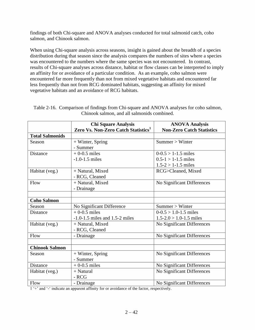
site which is frequently used but by small numbers of salmonids. Table 2-16 summarizes

2 – 42

findings of both Chi-square and ANOVA analyses conducted for total salmonid catch, coho

salmon, and Chinook salmon.

When using Chi-square analysis across seasons, insight is gained about the breadth of a species

distribution during that season since the analysis compares the numbers of sites where a species

was encountered to the numbers where the same species was not encountered. In contrast,

results of Chi-square analyses across distance, habitat or flow classes can be interpreted to imply

an affinity for or avoidance of a particular condition. As an example, coho salmon were

encountered far more frequently than not from mixed vegetative habitats and encountered far

less frequently than not from RCG dominated habitats, suggesting an affinity for mixed

vegetative habitats and an avoidance of RCG habitats.

Table 2-16. Comparison of findings from Chi-square and ANOVA analyses for coho salmon,

Chinook salmon, and all salmonids combined.

Chi Square Analysis

Zero Vs. Non-Zero Catch Statistics1

ANOVA Analysis

Non-Zero Catch Statistics

Total Salmonids

Season + Winter, Spring

- Summer

Summer > Winter

Distance + 0-0.5 miles

-1.0-1.5 miles

0-0.5 > 1-1.5 miles

0.5-1 > 1-1.5 miles

1.5-2 > 1-1.5 miles

Habitat (veg.) + Natural, Mixed

- RCG, Cleaned

RCG>Cleaned, Mixed

Flow + Natural, Mixed

- Drainage

No Significant Differences

Coho Salmon

Season No Significant Difference Summer > Winter

Distance + 0-0.5 miles

-1.0-1.5 miles and 1.5-2 miles

0-0.5 > 1.0-1.5 miles

1.5-2.0 > 1.0-1.5 miles

Habitat (veg.) + Natural, Mixed

- RCG, Cleaned


Flow - Drainage No Significant Differences

Chinook Salmon

Season + Winter, Spring

- Summer


Distance + 0-0.5 miles No Significant Differences

Habitat (veg.) + Natural

- RCG


Flow - Drainage No Significant Differences 1 „+‟ and „-„ indicate an apparent affinity for or avoidance of the factor, respectively.

2 – 43

Coho salmon at all juvenile life history stages were found to utilize agricultural waterways across

a wider range of seasons and habitat conditions (vegetation and flow classes) than juvenile

Chinook salmon. The abundant presence of coho salmon in virtually all habitat conditions

sampled during all seasons suggests a life history strategy that relies on agricultural waterways as

rearing habitat for extended periods.

In contrast, Chinook salmon appeared most likely to utilize agricultural waterways for spring-fall

rearing; Juvenile Chinook salmon were uncommonly encountered in agricultural waterways

during winter sampling, suggesting that they may utilize agricultural waterways much more

selectively than coho salmon. It has been shown that if non-winter rearing habitats are not

suitable for winter rearing, juvenile salmon may migrate to larger river systems to overwinter

(Bjornn 1978; Bjornn and Mallet 1964).

2.5.2.1 Temporal

Based on Chi-square analysis, salmonids in general (total salmonid catch) are most widely

distributed throughout agricultural waterways during winter and spring seasons and most

narrowly distributed during summer. When encountered however, the relative abundance of

salmonids followed an inverse trend, with summer catch rates being significantly greater than

winter catch rates (Table 2-16). Similar seasonal observations were made for coho salmon.

Although not statistically significant, coho salmon were most narrowly distributed during

summer sampling; when encountered however, catch rates of coho salmon were significantly

greater during summer than during winter.

Temporal variations in total salmonid and coho distributions and abundance are probably tied to

seasonal variations in water quality throughout the agricultural waterways, although immigration

and emigration timing of anadromous species from the agricultural waterways may partially

explain seasonal trends in salmonid distribution. Coho salmon make up the majority of the total

salmonid catch and therefore have a strong influence on trends observed for total salmonids. For

coho salmon, winter and spring samples include age 1+ fish which have been in the agricultural

waterways for as much as 9-10 months and, as such, have had substantial time to migrate

throughout the drainage system. In addition, observations made at the time of fish collection

indicated that water temperature is generally reduced and dissolved oxygen levels generally

increased during winter, potentially making agricultural waterways more suitable for widespread

salmonid rearing. Summer samples represent only age 0+ fish which would have been in the

drainage system for approximately 3 months (presumably ample time to migrate throughout the

drainage systems), but which are subject to reduced water quality conditions including probable

increased temperature and decreased dissolved oxygen. The limited distribution of coho during

summer is probably tied to reduced water quality, with fish localizing to areas of suitable

conditions for summer rearing. To the degree that localized habitat conditions impact water

quality (e.g. potentially increased BOD in areas heavily dominated by RCG or other in channel

vegetation), they may also impact the seasonal distribution of salmonids in agricultural

waterways.

Like other salmonids, Chinook salmon utilizing agricultural waterways were most widely

distributed during winter and spring and most narrowly distributed during summer. In contrast

to what was observed for other salmonids, catch rates of Chinook salmon where encountered

2 – 44

were notably lower in summer sampling events than in other seasons (although this was not

statistically significant; refer to Figure 2-16).

Based on these data continued adherence to King County public rule 21A-24 sub-sections 374

and 375 regarding the timing of maintenance activities and fish removal prior to such activity

(King County DDES 2001) is warranted. Although present within agricultural waterways during

the timelines delineated in that rule, salmonids are less widely distributed than at other times of

the year thereby minimizing the likelihood of encountering or disturbing salmonids during

maintenance activities. However, when found during this same timeframe, salmonids appear to

be more densely grouped indicating the need to conduct pre-maintenance fish removal activities

to ensure that impacts to salmonids, when present, are minimized.

2.5.2.2 Spatial

For coho salmon and total salmonid evaluations the distance that a sampling site was upstream

from the mouth of the drainage system which contained it was a significant factor in describing

both the likelihood of encountering salmonids as well as the abundance of salmonids which were

encountered. For Chinook salmon, distance was significant in defining the likelihood of

encountering the species, but was not significant in determining the abundance encountered if

present. Logically and in all cases, the likelihood of encountering salmonids was greatest for

sites nearest to the mouth of the drainage system (0-0.5 miles) and for coho salmon the

likelihood of encounter decreased directly with increased distance upstream. The likelihood of

encountering salmonids however did not appear to decrease directly with increased distance

upstream for either Chinook salmon or total salmonid evaluations.

Evaluation of catch rates of both combined salmonids and coho salmon across distance classes

also showed an unexpected pattern, with catch rates typically lowest within one of the

intermediate distance classes evaluated (1-1.5 miles upstream). Catch rates for both combined

salmonid and coho salmon were significantly greater in the furthest upstream distance class (1.5-

2.0 miles) than in the aforementioned distance class.

The unexpected and somewhat anomalous results for evaluations of the impacts of distance on

salmonid encounter and catch rates suggests that there is an interaction of distance with other

variables which is driving the statistical relevance of this factor in our analyses. Since the study

design did not allow for evaluation of interactions amongst variables of interest, further study is

warranted to better delineate the impact of upstream distance on salmonid distribution and catch

rates in agricultural waterways.

When considering all salmonids combined, the inclusion of cutthroat trout probably contributed

to this irregularity since cutthroat trout (either anadromous or resident) are likely associated to

some degree with higher gradient tributaries to agricultural waterways which are typically found

further upstream in the drainage systems. For Chinook salmon this irregularity suggests a

possible interaction between distance and habitat factors which could not be assessed during this

study.

2 – 45

2.5.2.3 Habitat Characteristics

In terms of frequency of use, salmonids (Chinook, coho and all combined) show a preference for

natural vegetative regimes and an apparent avoidance of RCG dominated habitats within

agricultural waterways. For coho and combined salmonids, a preference for mixed vegetative

habitats and avoidance of habitats recently cleaned of vegetation were also noted.

When considering only those sites where fish were encountered, combined salmonid densities

(catch rates) in RCG dominated habitats were significantly greater than in recently cleaned or

mixed vegetative habitats. Although not statistically significant, this same pattern of catch rates

was observed for coho salmon. When encountered, Chinook salmon catch rates exhibited a

slightly different pattern with highest catch rates observed in areas dominated by a natural

vegetative regime, and lowest catch rates observed in recently cleaned habitats; however, the

observed differences in catch rates of Chinook salmon across habitat types was not statistically

significant.

These demonstrated patterns of habitat use or avoidance by salmonids are important when

considering in-channel activities that may impact salmonids if and when they are present.

Encroachment by RCG into agricultural waterways which inhibits flow and may increase the

frequency and/or duration of flooding events is one of the primary reasons why landowners seek

to perform maintenance activities within King County‟s agricultural areas. Based on the

apparent avoidance of RCG dominated habitats by salmonids, maintenance activities aimed at

RCG removal, coupled with appropriate mitigation activities, may result in more preferred

habitats being made available to salmonids in these areas. It is important to note that there is an

apparent avoidance of „cleaned‟ (recently maintained) habitats by some salmonids suggesting

that maintenance activities may have a negative impact on habitat conditions in agricultural

waterways. However, the researchers believe that, given the apparent negative impact of

maintenance activities to salmonids, removal of RCG from agricultural waterways remains the

preferred alternative for long term benefits to salmonid populations in these systems for the

following reasons:

1. Effects of RCG encroachment into agricultural channels may have broader scale impacts

than maintenance activities. Very high RCG densities may inhibit immigration and

emigration to/from upstream areas as well as the area directly impacted by RCG. In

contrast, any negative habitat effects of maintenance activities are believed to remain

localized to the project area itself.

2. The potential negative impacts of „cleaned‟ habitats can be mitigated for through

vegetation plantings and introduction of temporary cover into channels to shorten and/or

minimize any negative impacts to salmonids.

3. The potential negative impacts of „cleaned‟ habitats are relatively short-lived, lasting only

until surrounding and/or in-channel vegetation can be re-established. In contrast, once

established, the negative impact of RCG encroachment is a relatively permanent impact

affecting salmonid populations.

4. Based on the relatively small extent of most maintenance projects (<0.5 waterway miles)

conducted in King County, the researchers believe that the mobility of salmonids will

allow them to easily access other more preferred habitat areas within the same drainage

system until positive impacts of mitigation measures are realized.

2 – 46

Based on these data continued adherence to King County public rule 21A-24 sub-section 383

(King County DDES 2001) regarding habitat mitigation following maintenance activities is

warranted. Mitigation measures should attempt to minimize re-establishment of RCG, resulting

in establishment of mixed or natural vegetative regimes preferred by salmonids. This would

likely be most effectively accomplished with measures described in subsections 383(b) and

383(c).

With regard to in channel habitat and cover, King County should consider the cost effectiveness

of measures described in subsection 383(a) regarding installation of in-channel structures (King

County DDES 2001). Subsection 383(b) calls for plantings to provide cover and shade to the

ditch or stream “during the first planting season after maintenance or at another time no later

than one year after completion of maintenance” thereby implying a very short term function of

any installed structures intended to do the same. Based on the apparent short term function and

relatively high cost of structures to be installed, King County might consider various alternatives

to this strategy including evaluation of more temporary and less costly alternatives to provide

short term cover following maintenance, or installation of structures only to waterways where

those measures described in subsection 383(b) would not be expected to provide substantive

shade or cover within the proposed timeframe.

Also based on these data, continued adherence to King County public rule 21A-24 sub-section

375 regarding fish removal prior to such activity (King County DDES 2001) is warranted. This

practice should continue to occur in all habitat configurations prior to scheduled maintenance

activities. Although less likely to be found in RCG dominated habitats than other habitats,

salmonids appear to be more densely grouped in RCG habitats when found. This indicates that

even though difficult, fish removal activities are necessary to ensure that impacts to salmonids,

when present, are minimized.

2.5.2.4 Flow Characteristics

Flow regime was not found to significantly influence the catch rates of Chinook or coho salmon

or all salmonids combined within agricultural waterways. The importance of flow regimes to

salmonids in agricultural waterways appears to be reflected in their frequency of use of various

flow regimes rather than the density of fish encountered.

In terms of frequency of use, salmonids (all combined) appear to prefer waterways with natural

or mixed flow regimes while avoiding those dominated by drainage flows. For individual

species (Chinook or coho salmon) the avoidance of channels dominated by drainage flow was

evident although no notable preference for other flow types was evident. Cutthroat trout are the

primary species encountered other than Chinook or coho salmon and probably drive the

differences in apparent preference or avoidance of various flow regimes between all salmonids

combined and individual species. Field observations suggest that channels dominated by

drainage flows tend to be smaller in size and have lower velocities than channels with different

flow regimes. Cutthroat trout found in agricultural waterways are frequently larger than other

species observed, and size of fish is often directly related to the size of channel (Bjornn and

Reiser 1991; Allen 1969) and focal velocity (Smith and Li 1983) preferred by salmonids,

potentially explaining the apparent affinity of mixed or natural flow regimes for all salmonids

combined.

2 – 47

2.6 Conclusions and Recommendations

Results of this study suggest that in relation to the tested hypothesis, salmonid density (as

indexed by capture frequency and/or catch rates) does vary temporally, spatially, and in relation

to physical factors such as surrounding vegetative regime and flow type in King County‟s

agricultural waterways. Specifics of that variation differ by species considered and have

previously been described in detail. However, general trends can be summarized as follows:

1. Temporally, salmonids tend to be least widely distributed but more concentrated during the

summer period, and most widely (but less densely) distributed during the winter and/or

spring periods.

2. Spatially, salmonids tend to be found more frequently and in greater abundance in close

proximity to the mouth of the drainage system in which they are collected. However, catch

frequency and catch rates do not appear to decline directly with increased distance from the

mouth. Findings suggest that there is an interaction of distance with other variables which is

driving the statistical relevance of this factor in our analyses.

3. Salmonids in agricultural waterways appear to avoid both habitats dominated by RCG and

those which have been recently cleaned/maintained, and appear to prefer habitats with a

mixed or natural vegetative regime.

4. Salmonids appear to avoid channels in which flows are dominated by drainage flow and lack

at least some component of natural flow. It remains somewhat unclear however if such

apparent avoidance is driven solely by flow source(s) or if variations in physical factors such

as channel size and flow velocity are responsible for this finding.

5. Findings of this study directly support the continued application of King County public rule

21A-24 sub-sections 374, 375, and 383(b) regarding maintenance timing, fish removal prior

to, and mitigation planting activities following maintenance activity (King County DDES

2001). Additionally, installation of short term cover following maintenance activities

(consistent with subsection 383(a) of the public rule) appears warranted based on findings of

this study although the cost effectiveness of measures currently described in that subsection

is unclear.

Based on the findings of this study component, recommendations for future work can be

summarized as follows:

1. Comparison of growth characteristics of salmonids in agricultural waterways relative to those

in natal or other types of rearing waters should be considered. Inquiry for salmonid growth

data from other areas in the Puget Sound area during this study did not locate any such data

for comparison. These comparisons would be valuable to help further define the relative

importance of agricultural waterways as salmonid habitat in King County.

2 – 48

2. King County should evaluate their desire or need to assess variations in salmonid use

and life history characteristics between APDs. This study was designed to assess

salmonid use and life history characteristics in agricultural areas as a whole and did

not consider potential differences between individual APDs. Data from this study

does provide baseline data suitable to aide in determining the need for such a study,

and/or clarifying design considerations of any such future study.

3. Further study should be considered to more clearly define the importance of distance

(above the waterway mouth) on salmonid use of agricultural waterways, including the

potential interaction of distance with other habitat variables (e.g. surrounding

vegetative regime, distance of waterway mouth to known spawning areas). Since the

current study design did not allow for evaluation of such interactions, and because

interpretation of significant findings regarding distance as it relates to salmonid

distribution and use of agricultural waterways was unclear, further study is warranted

to more clearly define the importance of distance on salmonid distribution and catch

rates in agricultural waterways.

4. It is recommended that King County independently assess the cost effectiveness of

measures currently described in public rule 21A-24, sub-section 383(a), as less

permanent and costly structures may meet the intended needs until such time as the

benefits of activities undertaken as part of subsection 383(b) are realized.

2 – 49

2.7 References

Allen, K.R. 1969. Limitations on production in salmonid populations in streams. Pages 1-18 in

Northcote, T.G. Editor. Symposium on salmon and trout in streams. H.R. MacMillan

Lectures in Fisheries. University of British Columbia, Institute of Fisheries. Vancouver.

Bell, M. C. 1991. Fisheries Handbook of Engineering Requirements and Biological Criteria.

Portland: U.S. Army Corps of Engineers.

Berge, H. B. 2002. 2001 Annual Monitoring Report. King County Agricultural Drainage

Assistance Program. King County Department of Natural Resources and Parks.

Available at: ftp://dnr.metrokc.gov/dnr/library/2002/kcr763.pdf

Berge, Hans, KCDNRP, personal communication with Tom Cichosz, June 20, 2005.

Berge, Hans, KCDNRP personal communication with Tom Cichosz, February, 2005.

Berge, Hans, KCDNRP, personal communication with Tom Cichosz. Date unknown.

Bjornn, T.C. 1978. Survival, production and yield of trout and Chinook salmon in the Lemhi

River, Idaho. University of Idaho, College of Forestry, Wildlife and Range Sciences

Bulletin 27. Moscow, Idaho.

Bjornn, T.C. and J. Mallet. 1964. Movements of planted and wild trout in an Idaho river system.

Transactions of the American Fisheries Society 93:70-76.

Bjornn, T. C. and D. W. Reiser. 1991. Habitat Requirements of Salmonids in Streams. In:

Influences of Forest and Rangeland Management on Salmonid Fishes and Their Habitats.

M. R. Meehan, Ed. Bethesda, MD: American Fisheries Society Special Publications, pp.

83-138.

Brun, C. 2003. Juvenile fall Chinook salmon coded wire tagging feasibility study in the

Deschutes River, Oregon. Confederated Tribes of the Warm Springs Reservation,

Oregon.

Carrasco, Ken, KCDNRP, personal communication with Tom Cichosz, September 28, 2001.

Connor, W.P. 1998. Emergence, Rearing, and Seaward Migration Timing of Natural

Subyearling Fall Chinook Salmon in the Snake River in 1998. United States Fish And

Wildlife Service, Idaho Fishery Resource Office. Ahsahka, Idaho.

Cramer, S.P. and J.T. Martin. 1978. Rogue basin evaluation program, juvenile progress report.

Oregon Department of Fish and Wildlife. Fish Research Project DACW-57-75-C-0109.

Annual Progress Report. Portland.

2 – 50

Grette, G.B. and C.D. Salo. 1986. The status of anadromous fishes of the Green/Duwamish

River system. Submitted to U.S. Army Corp of Engineers, Seattle District, Seattle,

Washington. 413 p.

Hillman, T.W., J.S. Griffith, and W.S. Platts. 1987. The effects of sediment on summer and

winter habitat selection by juvenile Chinook salmon in an Idaho stream. Transactions of

the American Fisheries Society 116:185-195.

Johnson, O.W., M.H. Ruckelshaus, W.S. Grant, F.W. Waknitz, A.M. Garrett, G.J. Bryant, K.

Neely, and J.J. Hard. 1999. Status review of coastal cutthroat trout from Washington,

Oregon, and California. U.S. Dept. Commer., NOAA Tech. Memo. NMFS-NWFSC-37,

292 p.

King County Department of Development and Environmental Services (DDES). 2001. Public

Rules Chapter 21A-24. Sensitive areas: Maintenance of agricultural ditches and streams

used by salmonids.

Koski, K.V. 1966. The survival of coho salmon (Oncorhynchus kisutch) from egg deposition to

emergence in three Oregon coastal streams. M.S. Thesis. Oregon State University.

Meehan, W. R. and T. C. Bjornn. 1991. Salmonid Distributions and Life Histories. In: Influences

of Forest and Rangeland Management on Salmonid Fishes and Their Habitats. W. R.

Meehan, Ed. Bethesda, MD: American Fisheries Society Special Publication, pp. 47-82.

Myers, J. M., Kope, R. G., Bryant, G. J., Teel, D., Lierheimer, L. J., Wainright, T. C., Grant, W.

S., Waknitz, F. W., Neely, K.; Lindley, S. T. 1998. Status Review of Chinook Salmon

from Washington, Idaho, Oregon, and California. Seattle: National Marine Fisheries

Service. Technical Memorandum NMFS-NWFSC-35.

National Marine Fisheries Service. 2000. Guidelines for Electrofishing Waters Containing

Salmonids Listed Under the Endangered Species Act. 5pp.

Ney, J.J. 1993. Practical use of biological statistics. Pages 137-158 in Kohler, C.C. and Hubert,

W.A., Editors. Inland fisheries management in North America. Bethesda, MD: American

Fisheries Society.

Raleigh, R. F., W. J. Miller, and P. C. Nelson. 1986. Habitat Suitability Index Models and

Instream Flow Suitability Curves: Chinook Salmon. Fish and Wildlife Service, U. S.

Department of the Interior.

Ramseyer, L.J. 1995. Total length to fork length relationships of juvenile hatchery-reared coho

and Chinook salmon. The Progressive Fish-Culturist 57:250-251.

2 – 51

Reiser, D.W. and R.G. White. 1981. Effects of flow fluctuation and redd dewatering on

salmonid embryo development and fry quality. Idaho Water and Energy Resources

Research Institute. Technical research completion report, contract DE-AC79-

79BP10848.

SAS Institute. 2006. SAS/STAT® Software. Providing the foundation for SAS’ analytics.

Website accessed November 17, 2006.

<http://www.sas.com/technologies/analytics/statistics/stat/index.html>.

Smith, A.K. 1973. Development and application of spawning velocity and depth criteria for

Oregon salmonids. Transactions of the American Fisheries Society 102:312-316.

Smith, J.J. and H.W. Li. 1983. Energetic factors influencing foraging tactics of juvenile

steelhead trout, Salmo gairdneri. Pages 173-180 in L.L.G. Noakes, D.G. Lindquist, G.S.

Helfman, and J.A. Ward, editors. Predators and prey in fishes. Dr. W. Junk, The Hague,

Netherlands.

Thompson, K. 1972. Determining Stream Flows for Fish Life. Proceedings, Instream Flow

Requirements Workshop. Vancouver, WA: Pacific Northwest River Basins Commission.

Triton Environmental Consultants Ltd. 2001. Fry emergence project 1999, Nechako fisheries

conservation program. Technical Report No. M98-6.

Tschaplinski, P.J. and G.F. Hartman. 1983. Winter distribution of juvenile coho salmon

(Oncorhynchus kisutch) before and after logging in Carnation Creek, British Columbia,

and some implications for overwinter survival. Canadian Journal of Fisheries and

Aquatic Sciences 40:452-461.

Van Den Avyle, M.J. 1993. Dynamics of exploited fish populations. Pages 105-136 in C.C.

Kohler and S.A. Hubert, editors. Inland fisheries management in North America.

American Fisheries Society, Bethesda, Maryland.

Washington Department of Fish and Wildlife. 1995. Documents submitted to the ESA

Administrative Record for west coast Chinook salmon by B. Tweit. (Available from the

Environmental and Technical Services Division, NMFS, Portland, OR).

Washington Department of Fish and Wildlife. 1997. Policy of Washington Department of Fish

and Wildlife and the Western Washington Treaty Tribes concerning wild salmonids.

Washington State Department of Fish and Wildlife, Olympia, WA. 43p.

Washington State University and University of Washington. 2006. A Study of Agricultural

Drainage in the Puget Sound Lowlands to Determine Practices which Minimize

Detrimental Effects on Salmonids: Sampling and Analysis Plan. Prepared for the King

County Department of Natural Resources and Parks, Water and Land Resources

Division.

2 – 52

Weitkamp, L.A., T.C. Wainwright, G.J. Bryant, G.B. Milner, D.J. Teel, R.G. Kope and R.S.

Waples. 1995. Status Review of Coho Salmon from Washington, Oregon, and California.

Seattle: National Marine Fisheries Service. Technical Memorandum NMFS-NWFSC-24.

Williams, R.W., R.M. Laramie, and J.J. Ames. 1975. A Catalog of Washington Streams and

Salmon Utilization. Volume 1. Puget Sound Region. Washington Department of

Fisheries.

2 – 53

Appendix 2-A: Coho Salmon Seasonal Length Frequency Graphs

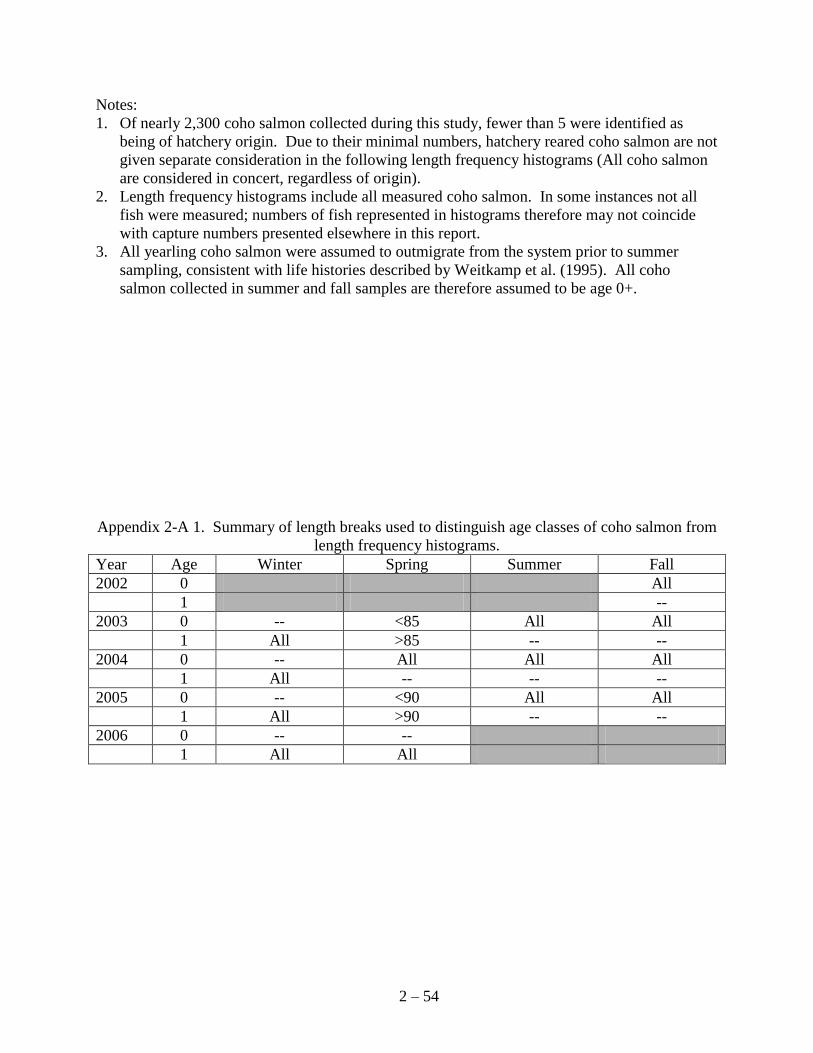
2 – 54

Notes:

1. Of nearly 2,300 coho salmon collected during this study, fewer than 5 were identified as

being of hatchery origin. Due to their minimal numbers, hatchery reared coho salmon are not

given separate consideration in the following length frequency histograms (All coho salmon

are considered in concert, regardless of origin).

2. Length frequency histograms include all measured coho salmon. In some instances not all

fish were measured; numbers of fish represented in histograms therefore may not coincide

with capture numbers presented elsewhere in this report.

3. All yearling coho salmon were assumed to outmigrate from the system prior to summer

sampling, consistent with life histories described by Weitkamp et al. (1995). All coho

salmon collected in summer and fall samples are therefore assumed to be age 0+.

Appendix 2-A 1. Summary of length breaks used to distinguish age classes of coho salmon from

length frequency histograms.

Year Age Winter Spring Summer Fall

2002 0 All

1 --

2003 0 -- <85 All All

1 All >85 -- --

2004 0 -- All All All

1 All -- -- --

2005 0 -- <90 All All

1 All >90 -- --

2006 0 -- --

1 All All

2 – 55

October 2002

0

5

10

15

20

25

30

35

40

45

30

35

40

45

50

55

60

65

70

75

80

85

90

95

100

105

110

115

120

125

130

135

140

145

>145

Max. Length (mm)

Count

Coho

Appendix 2-A 2. Length frequency histogram of coho salmon collected during October, 2002.

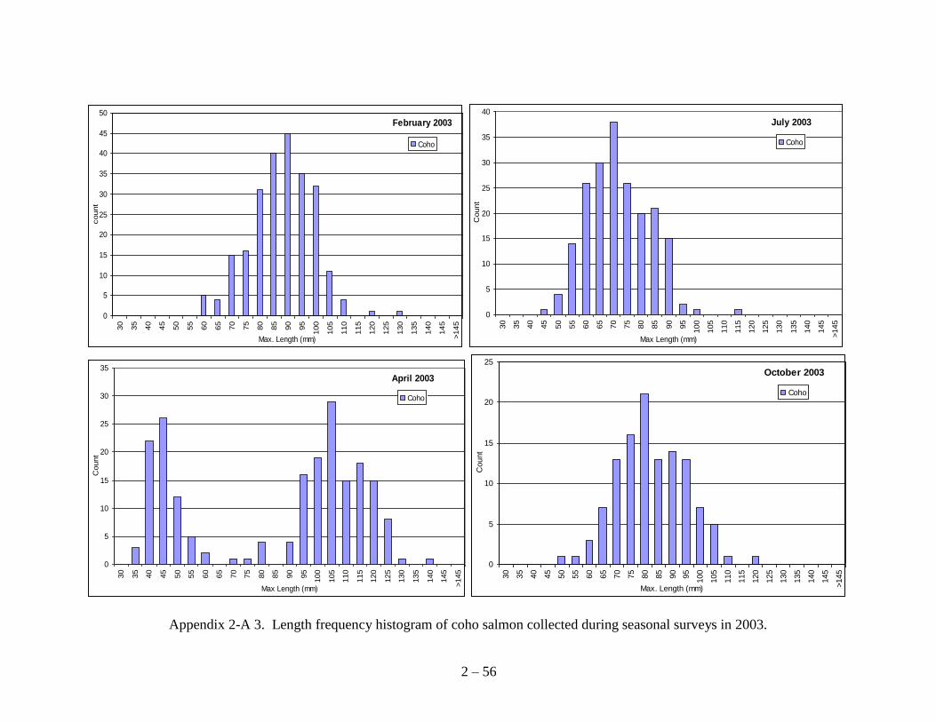
2 – 56

February 2003

0

5

10

15

20

25

30

35

40

45

5030

35

40

45

50

55

60

65

70

75

80

85

90

95

100

105

110

115

120

125

130

135

140

145

>145

Max. Length (mm)

count

Coho

July 2003

0

5

10

15

20

25

30

35

40

30

35

40

45

50

55

60

65

70

75

80

85

90

95

100

105

110

115

120

125

130

135

140

145

>145

Max Length (mm)

Count

Coho

April 2003

0

5

10

15

20

25

30

35

30

35

40

45

50

55

60

65

70

75

80

85

90

95

100

105

110

115

120

125

130

135

140

145

>145

Max Length (mm)

Count

Coho

October 2003

0

5

10

15

20

25

30

35

40

45

50

55

60

65

70

75

80

85

90

95

100

105

110

115

120

125

130

135

140

145

>145

Max. Length (mm)

Count

Coho

Appendix 2-A 3. Length frequency histogram of coho salmon collected during seasonal surveys in 2003.

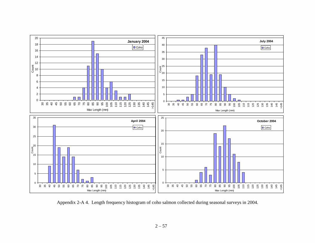
2 – 57

January 2004

0

2

4

6

8

10

12

14

16

18

20

30

35

40

45

50

55

60

65

70

75

80

85

90

95

100

105

110

115

120

125

130

135

140

145

>145

Max Length (mm)

Count

Coho

July 2004

0

5

10

15

20

25

30

35

40

45

30

35

40

45

50

55

60

65

70

75

80

85

90

95

100

105

110

115

120

125

130

135

140

145

>145

Max Length (mm)

Count

Coho

April 2004

0

5

10

15

20

25

30

35

30

35

40

45

50

55

60

65

70

75

80

85

90

95

100

105

110

115

120

125

130

135

140

145

>145

Max Length (mm)

Count

Coho

October 2004

0

5

10

15

20

25

30

35

40

45

50

55

60

65

70

75

80

85

90

95

100

105

110

115

120

125

130

135

140

145

>145

Max Length (mm)

Count

Coho


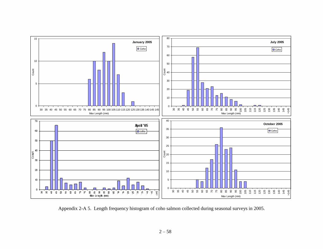
2 – 58

January 2005

0

5

10

15

30 35 40 45 50 55 60 65 70 75 80 85 90 95 100 105 110 115 120 125 130 135 140 145 145

Max Length (mm)

Count

Coho

July 2005

0

10

20

30

40

50

60

70

80

30

35

40

45

50

55

60

65

70

75

80

85

90

95

100

105

110

115

120

125

130

135

140

145

>145

Max Length (mm)

Count

Coho

October 2005

0

5

10

15

20

25

30

35

40

30

35

40

45

50

55

60

65

70

75

80

85

90

95

100

105

110

115

120

125

130

135

140

145

>145

Max Length (mm)

Count

Coho


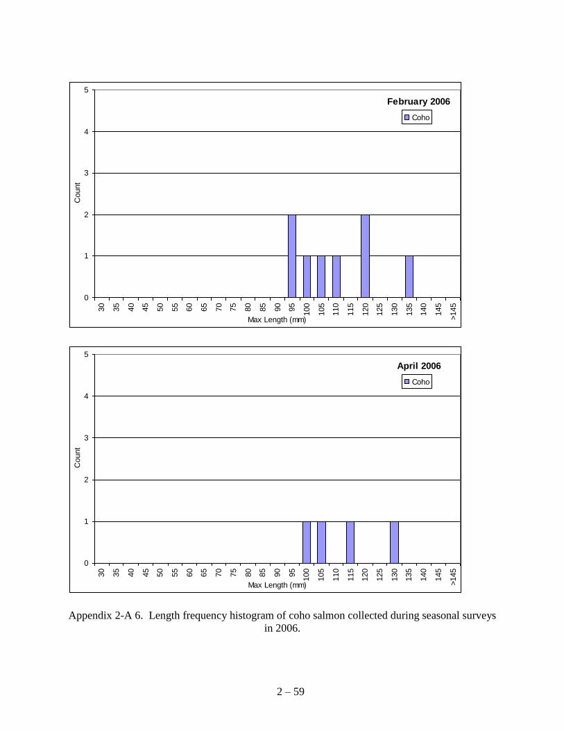
2 – 59

February 2006

0

1

2

3

4

5

30

35

40

45

50

55

60

65

70

75

80

85

90

95

100

105

110

115

120

125

130

135

140

145

>145

Max Length (mm)

Count

Coho

April 2006

0

1

2

3

4

5

30

35

40

45

50

55

60

65

70

75

80

85

90

95

100

105

110

115

120

125

130

135

140

145

>145

Max Length (mm)

Count

Coho

Appendix 2-A 6. Length frequency histogram of coho salmon collected during seasonal surveys

in 2006.

2 – 60

Appendix 2-B: Chinook Salmon Seasonal Length Frequency Graphs.

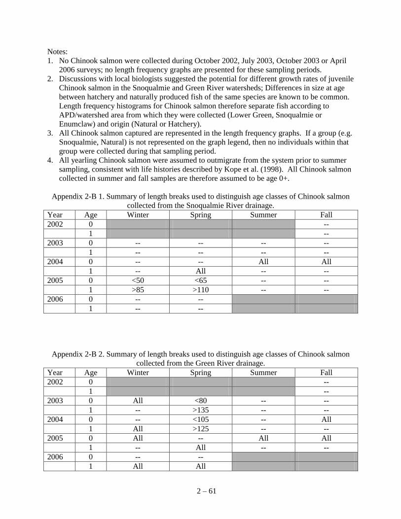
2 – 61

Notes:

1. No Chinook salmon were collected during October 2002, July 2003, October 2003 or April

2006 surveys; no length frequency graphs are presented for these sampling periods.

2. Discussions with local biologists suggested the potential for different growth rates of juvenile

Chinook salmon in the Snoqualmie and Green River watersheds; Differences in size at age

between hatchery and naturally produced fish of the same species are known to be common.

Length frequency histograms for Chinook salmon therefore separate fish according to

APD/watershed area from which they were collected (Lower Green, Snoqualmie or

Enumclaw) and origin (Natural or Hatchery).

3. All Chinook salmon captured are represented in the length frequency graphs. If a group (e.g.

Snoqualmie, Natural) is not represented on the graph legend, then no individuals within that

group were collected during that sampling period.

4. All yearling Chinook salmon were assumed to outmigrate from the system prior to summer

sampling, consistent with life histories described by Kope et al. (1998). All Chinook salmon

collected in summer and fall samples are therefore assumed to be age 0+.

Appendix 2-B 1. Summary of length breaks used to distinguish age classes of Chinook salmon

collected from the Snoqualmie River drainage.


2002 0 --

1 --

2003 0 -- -- -- --

1 -- -- -- --

2004 0 -- -- All All

1 -- All -- --

2005 0 <50 <65 -- --

1 >85 >110 -- --

2006 0 -- --

1 -- --

Appendix 2-B 2. Summary of length breaks used to distinguish age classes of Chinook salmon

collected from the Green River drainage.


2002 0 --

1 --

2003 0 All <80 -- --

1 -- >135 -- --

2004 0 -- <105 -- All

1 All >125 -- --

2005 0 All -- All All

1 -- All -- --

2006 0 -- --

1 All All

2 – 62

Chinook

February 2003

0

1

2

3

4

5

30 35 40 45 50 55 60 65 70 75 80 85 90 95 100 105 110 115 120 125 130 135 140 145 >145

Max Length (mm)

Count

Green River, Natural

Chinook

April 2003

0

1

2

3

4

5

30 35 40 45 50 55 60 65 70 75 80 85 90 95 100 105 110 115 120 125 130 135 140 145 >145

Max Length (mm)

Count


Green River, Hatchery

Appendix 2-B 3. Length frequency histogram of Chinook salmon collected during seasonal

surveys in 2003.

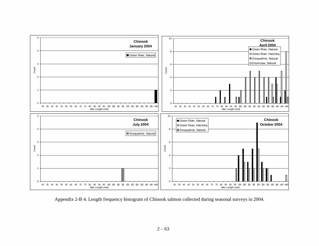
2 – 63

Chinook

January 2004

0

1

2

3

4

5

30 35 40 45 50 55 60 65 70 75 80 85 90 95 100 105 110 115 120 125 130 135 140 145 >145

Max Length (mm)

Count


Chinook

April 2004

0

2

4

6

8

10

30 35 40 45 50 55 60 65 70 75 80 85 90 95 100 105 110 115 120 125 130 135 140 145 >145

Max Length (mm)

Count



Snoqualmie, Natural

Enumclaw, Natural

Chinook

July 2004

0

1

2

3

4

5

30 35 40 45 50 55 60 65 70 75 80 85 90 95 100 105 110 115 120 125 130 135 140 145 >145

Max Length (mm)

Count

Snoqualmie, Natural

Chinook

October 2004

0

2

4

6

8

10

30 35 40 45 50 55 60 65 70 75 80 85 90 95 100 105 110 115 120 125 130 135 140 145 >145

Max Length (mm)

Count



Snoqualmie, Natural

Appendix 2-B 4. Length frequency histogram of Chinook salmon collected during seasonal surveys in 2004.

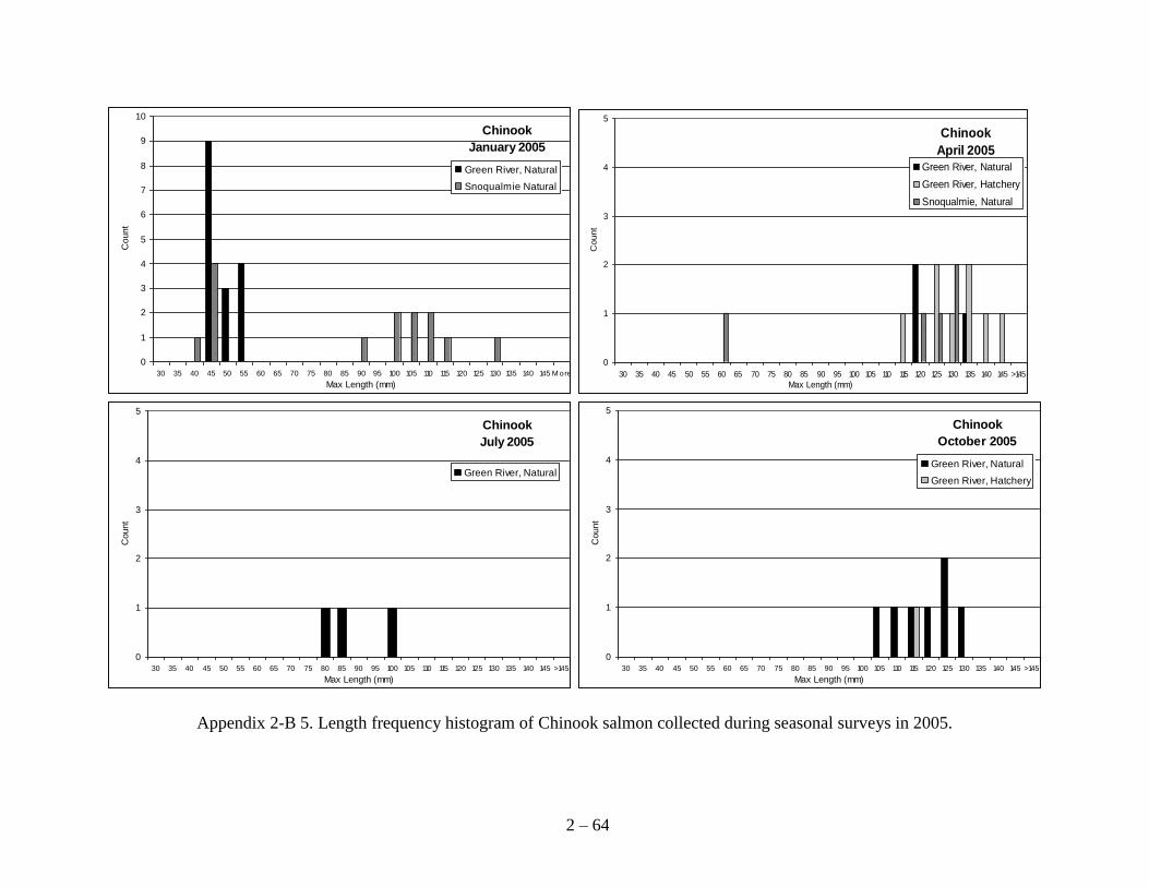
2 – 64

Chinook

January 2005

0

1

2

3

4

5

6

7

8

9

10

30 35 40 45 50 55 60 65 70 75 80 85 90 95 100 105 110 115 120 125 130 135 140 145 M ore

Max Length (mm)

Count


Snoqualmie Natural

Chinook

April 2005

0

1

2

3

4

5

30 35 40 45 50 55 60 65 70 75 80 85 90 95 100 105 110 115 120 125 130 135 140 145 >145

Max Length (mm)

Count



Snoqualmie, Natural

Chinook

July 2005

0

1

2

3

4

5

30 35 40 45 50 55 60 65 70 75 80 85 90 95 100 105 110 115 120 125 130 135 140 145 >145

Max Length (mm)

Count


Chinook

October 2005

0

1

2

3

4

5

30 35 40 45 50 55 60 65 70 75 80 85 90 95 100 105 110 115 120 125 130 135 140 145 >145

Max Length (mm)

Count



Appendix 2-B 5. Length frequency histogram of Chinook salmon collected during seasonal surveys in 2005.

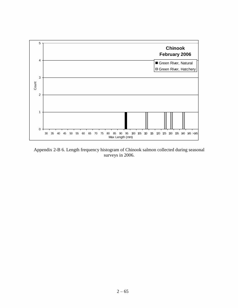
2 – 65

Chinook

February 2006

0

1

2

3

4

5

30 35 40 45 50 55 60 65 70 75 80 85 90 95 100 105 110 115 120 125 130 135 140 145 >145

Max Length (mm)

Count



Appendix 2-B 6. Length frequency histogram of Chinook salmon collected during seasonal

surveys in 2006.