Chapter 2: Data - Mrs. Krummelmrskrummel.com/documents/BVD_chapter_notes.pdf · Stats: Modeling the World – Chapter 2 ... Chapter 2 Chapter 2: Data What are data? ... B 45 for 151

Stats: Modeling the World – Chapter 2

Chapter 2: Data

What are data?

In order to determine the context of data, consider the “W’s” Who –

What (and in what units) –

When –

Where –

Why –

How –

There are two major ways to treat data: A _______________ _______________ is used to answer questions about how cases fall into

categories. A categorical variable may be comprised of word labels, or it may use numbers as labels.

Examples:

A _______________ _______________ is used to answer questions about the quantity of what is being measured. A quantitative variable is comprised of numeric values.

Examples:

What is a statistic?

Are the numbers 17, 21, 44, 76 data?

Data must have ______ to be meaningful. The numbers listed above could be test scores, ages of agroup of golfers, or the uniform numbers of the starting backfield on the football team. Without ______data cannot be interpreted.


Suppose a Consumer Reports article (published in June 2005) on energy bars gave the brand name, flavor, price, number of calories, and grams of protein and fat. Identify the following:

Who:

What:

When:

Where:

How:

Why:

Categorical variables:

Quantitative variables (with units):

A report on the Boston Marathon listed each runner’s gender, county, age, and time. Identify the following:

Who:

What:

When:

Where:

How:

Why:

Categorical variables:

Quantitative variables (with units):


Chapter 2: Data

What are data?Data are values along with their context. Data can be numbers or labels.

In order to determine the context of data, consider the “W’s” Who – the cases (about whom the data was collected). People are referred to as respondents,

subjects, or participants, while objects are referred to as experimental units.

What (and in what units) – the variables recorded about each individual.

When – when the data was collected.

Where – where the data was collected.

Why – why the data was collected. This can determine whether a variable is treated as categorical or quantitative.

How – how the data was collected.

There are two major ways to treat data: categorical and quantitative. A categorical variable names categories and is used to answer questions about how cases fall

into those categories. A categorical variable may be comprised of word labels, or it may use numbers as labels.

A quantitative variable is used to answer questions about the quantity of what is being measured. A quantitative variable is comprised of numeric values.

What is a statistic? A statistic is a numerical summary of data.

17, 21, 44, 76

Are the numbers listed above data? Data must have context to be meaningful. The numbers listed above could be test scores, ages of a group of golfers, or the uniform numbers of the starting backfield on the football team. Without context, data cannot be interpreted.

Suppose a Consumer Reports article (published in June 2005) on energy bars gave the brand name, flavor, price, number of calories, and grams of protein and fat. Identify the following:

Who: energy bars

What: brand, flavor, price, calories, protein, fat

When: not specified

Where: not specified

How: not specified (nutrition label? laboratory testing?)

Why: to inform potential consumers

Categorical variables: brand, flavor


Quantitative variables (with units): price (US$), number of calories (calories), protein (grams), fat (grams)

A report on the Boston Marathon listed each runner’s gender, county, age, and time. Identify the following:

Who: Boston Marathon runners

What: gender, county, age, time

When: not specified

Where: Boston

How: not specified (registration information?)

Why: race result reporting

Categorical variables: gender, county

Quantitative variables (with units): age (years), time (hours, minutes, seconds)


Chapter 3 – Displaying and Describing Categorical Data

_______________ _______________ are often used to organize categorical data. Frequency tables display the category names and the _______________ of the number of data values in each category._ _______________________ also display the category names, but they give the

_______________ rather than the counts for each category.

Color Freq. Rel. Freq. PercentBlue 13Red 7

Orange 11Green 9Yellow 8Brown 7TOTAL 55 1.000 100%

A _______________ is often used to display categorical data. The height of each bar represents the _______________ for each category. Bars are displayed next to each other for easy comparison. When constructing a bar chart, note that the bars do not _______________ one another. Categorical variables usually cannot be ordered in a meaningful way; therefore the order in which the bars are displayed is often meaningless.

A _________ bar chart displays the proportion of counts for each category.

The sum of the relative frequencies is _____.

A _______________ _______________ is another type of display used to show categorical data. Pie charts show parts of a whole. Pie charts are often difficult to construct by hand.

A _______________ _______________ shows two categorical variables together. The margins give the frequency distributions for each of the variables, also called the ________ ___ .

M&M Color Distribution

13

7

11

98

7

0

2

4

6

8

10

12

14

Blue Red Orange Green Yellow Brown

Fre

qu

enc

y


24%

13%

20%

16%14% 13%

0%

5%

10%

15%

20%

25%

30%


Fre

qu

enc

y


Examine the class data about gender and political view – liberal, moderate, conservative.

Liberal Moderate Conservative TOTAL

Male

Female

TOTAL

What percent of the class are girls with liberal political views?

What percent of the liberals are girls?

What percent of the girls are liberals?

What is the marginal distribution of gender?

What is the marginal distribution of political views?

A conditional distribution shows the distribution of one variable for only the individuals who satisfy some condition on another variable.

The conditional distribution of political preference, conditional on being male:Liberal Moderate Conservative TOTAL

Male

The conditional distribution of political preference, conditional on being female:Liberal Moderate Conservative TOTAL

Female

What is the conditional relative frequency distribution of gender among conservatives?

If the conditional distributions are the same, we can conclude that the variables are not associated. Therefore, they are _______________ of one another.

If the conditional distributions differ, we can conclude that the variables are somehow associated. Therefore, they are _______________ of one another.

Are gender and political view independent?


A segmented bar chart displays the same information as a pie chart, but in the form of bars instead of circles. Comparing segmented bar charts is a good way to tell if two variables are independent of one another or not.

Gender vs. Political Preference

0%

10%

20%

30%

40%

50%

60%

70%

80%

90%

100%

Male Female

Per

cen

t

Explain how the graph on the left violates the “area principle.”

Explain what is wrong with the graph below.


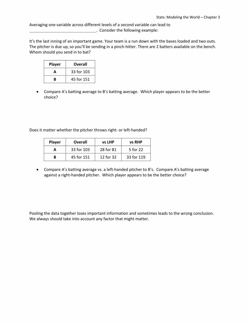
Averaging one variable across different levels of a second variable can lead to ______________________________. Consider the following example:

It’s the last inning of an important game. Your team is a run down with the bases loaded and two outs. The pitcher is due up, so you’ll be sending in a pinch-hitter. There are 2 batters available on the bench. Whom should you send in to bat?

Player Overall

A 33 for 103

B 45 for 151

Compare A’s batting average to B’s batting average. Which player appears to be the better choice?

Does it matter whether the pitcher throws right- or left-handed?

Player Overall vs LHP vs RHP

A 33 for 103 28 for 81 5 for 22

B 45 for 151 12 for 32 33 for 119

Compare A’s batting average vs. a left-handed pitcher to B’s. Compare A’s batting average against a right-handed pitcher. Which player appears to be the better choice?

Pooling the data together loses important information and sometimes leads to the wrong conclusion. We always should take into account any factor that might matter.


Notes: Displaying and Describing Categorical Data

Frequency tables are often used to organize categorical data. Frequency tables display the category names and the counts of the number of data values in each category. Relative frequency tables also display the category names, but they give the percentages rather than the counts for each category.

Color Freq. Rel. Freq. PercentBlue 13 0.236 24%Red 7 0.127 13%

Orange 11 0.200 20%Green 9 0.164 16%Yellow 8 0.145 14%Brown 7 0.127 13%TOTAL 55 1.000 100%

A bar chart is often used to display categorical data. The height of each bar represents the count for each category. Bars are displayed next to each other for easy comparison. When constructing a bar chart, note that the bars do not touch one another. Categorical variables usually cannot be ordered in a meaningful way; therefore the order in which the bars are displayed is often meaningless.

A relative frequency bar chart displays the proportion of counts for each category.

The sum of the relative frequencies is 100%.

A pie chart is another type of display used to show categorical data. Pie charts show parts of a whole. Pie charts are often difficult to construct by hand.

A contingency table shows two categorical variables together. The margins give the frequency distributions for each of the variables, also called the marginal distribution.


13

7

11

98

7

0

2

4

6

8

10

12

14


Fre

qu

enc

y


24%

13%

20%

16%14% 13%

0%

5%

10%

15%

20%

25%

30%


Fre

qu

enc

y


Examine the class data about gender and political view – liberal, moderate, conservative.

Liberal Moderate Conservative TOTAL

Male

Female

TOTAL

What percent of the class are girls with liberal political views?

What percent of the liberals are girls?

What percent of the girls are liberals?

What is the marginal distribution of gender?

What is the marginal distribution of political views?

A conditional distribution shows the distribution of one variable for only the individuals who satisfy some condition on another variable.

The conditional distribution of political preference, conditional on being male:Liberal Moderate Conservative TOTAL

Male

The conditional distribution of political preference, conditional on being female:Liberal Moderate Conservative TOTAL

Female

What is the conditional relative frequency distribution of gender among conservatives?

If the conditional distributions are the same, we can conclude that the variables are not associated. Therefore, they are independent of one another.

If the conditional distributions differ, we can conclude that the variables are somehow associated. Therefore, they are not independent of one another.

Are gender and political view independent?


A segmented bar chart displays the same information as a pie chart, but in the form of bars instead of circles. Comparing segmented bar charts is a good way to tell if two variables are independent of one another or not.

Gender vs. Political Preference

0%

10%

20%

30%

40%

50%

60%

70%

80%

90%

100%

Male Female

Per

cen

t

Explain how the graph on the left violates the “area principle.”

Explain what is wrong with the graph below.


Averaging one variable across different levels of a second variable can lead to Simpson’s Paradox. Consider the following example:

It’s the last inning of an important game. Your team is a run down with the bases loaded and two outs. The pitcher is due up, so you’ll be sending in a pinch-hitter. There are 2 batters available on the bench. Whom should you send in to bat?

Player Overall

A 33 for 103

B 45 for 151

Compare A’s batting average to B’s batting average. Which player appears to be the better choice? Player A has a higher batting average (0.320 vs. 0.298), so he looks like the better choice.

Does it matter whether the pitcher throws right- or left-handed? Player Overall vs LHP vs RHP

A 33 for 103 28 for 81 5 for 22

B 45 for 151 12 for 32 33 for 119

Compare A’s batting average vs. a left-handed pitcher to B’s. Compare A’s batting average against a right-handed pitcher. Which player appears to be the better choice?Player B has a higher batting average against both right- and left-handed pitching, even though his overall average is lower. Player B hits better against both right- and left-handed pitchers. So no matter the pitcher, B is a better choice. So why is his batting “average” lower? Because B sees a lot more right-handed pitchers than A, and (at least for these guys) right-handed pitchers are harder to hit. For some reason, A is used mostly against left-handed pitchers, so A has a higher average.

Pooling the data together loses important information and leads to the wrong conclusion. We always should take into account any factor that might matter.


Notes: Displaying Quantitative Data

A _______________ or _______________ is often used to display categorical data. These types of displays, however, are not appropriate for quantitative data. Quantitative data is often displayed using either a _______________ _______________ or a _______________

In a histogram, the interval corresponding to the width of each bar is called a _______________ A histogram displays the bin counts as the height of the bars (like a bar chart). Unlike a bar chart, however, the bars in a histogram _______________ one another. An empty space between bars represents a _______________ in data values. If a value falls on the border between two consecutive bars, it is placed in the bin on the _______________.

Shoe Sizes of AP Stat Students

6 6.5 7 7.5 8 8.5 9 9.5 10 10.5 11 11.5 12 12.5 13

Shoe Size

# o

f S

tud

en

ts

A _______________ _______________ histogram displays the proportion of cases in each bin instead of the count.

Histograms are useful when _____________________________________________, and they can easily be constructed using a graphing calculator. A disadvantage of histograms is that they _____________________________________________.

Be sure to choose an appropriate bin width when constructing a histogram. As a general rule of thumb, your histogram should contain about _______ bars.

A _______________ _______________ is similar to a histogram, but it shows______________________________ rather than bars. It may be necessary to _______________ stems if the range of data values is small.


Number of Pairs of Shoes Owned

00112233

KEY:

A _______________ _______________ stem-and-leaf plot can be useful when _______________ two distributions.


Male Female .00112233

KEY:

The stems of the stem-and-leaf plot correspond to the _______________ of a histogram. You may only use ______ digit for the leaves. Round or truncate your values if necessary.

Stem-and-leaf plots are useful when working with sets of data that are __________________ __________________ in size, and when you want to display _______________ _______________.

How would you setup the following stem-and-leaf plots?

quiz scores (out of 100)

student GPA’s

student weights

SAT scores

weights of cattle (1000-2000 pounds)


_______________ may also be used to display quantitative variables. Dot plots are useful when working with ____________ sets of data.

Guess Your Teacher's Age

25 26 27 28 29 30 31 32 33 34 35 36 37 38 39 40

Predicted Age

When describing a distribution, you should tell about three things: _______________ , _______________, and _______________. You should also mention any unusual features, like _______________ or _______________.

Identify the shapes of the following distributions:

When comparing two or more distributions, compare the _______________ , _______________, and _______________, and compare any _______________ features. It is important, when comparing distributions, that their graphs be constructed using the same _______________.

You can sometimes make a skewed distribution appear more symmetric by _______________ (or transforming) your data.


Notes: Displaying Quantitative Data

A bar chart or pie chart is often used to display categorical data. These types of displays, however, are not appropriate for quantitative data. Quantitative data is often displayed using either a histogram, dot plot, or a stem-and-leaf plot.

In a histogram, the interval corresponding to the width of each bar is called a bin. A histogram displays the bin counts as the height of the bars (like a bar chart). Unlike a bar chart, however, the bars in a histogram touch one another. An empty space between bars represents a gap in data values. If a value falls on the border between two consecutive bars, it is placed in the bin on the right.

Shoe Sizes of AP Stat Students

6 6.5 7 7.5 8 8.5 9 9.5 10 10.5 11 11.5 12 12.5 13

Shoe Size

# o

f S

tud

en

ts

A relative frequency histogram displays the proportion of cases in each bin instead of the count.

Histograms are useful when working with large sets of data, and they can easily be constructed using a graphing calculator. A disadvantage of histograms is that they do not show individual values.

Be sure to choose an appropriate bin width when constructing a histogram. As a general rule of thumb, your histogram should contain about 10 bars.

A stem-and-leaf plot is similar to a histogram, but it shows individual values rather than bars. It may be necessary to split stems if the range of data values is small.


00112233

KEY:


A back-to-back stem-and-leaf plot can be useful when comparing two distributions.


Male Female .00112233

KEY:

The stems of the stem-and-leaf plot correspond to the bins of a histogram. You may only use one digit for the leaves. Round or truncate your values if necessary.

Stem-and-leaf plots are useful when working with sets of data that are small to moderate in size, and when you want to display individual values.

How would you setup the following stem-and-leaf plots?

quiz scores (out of 100)

student GPA’s

student weights

SAT scores

weights of cattle (1000-2000 pounds)

Dot plots may also be used to display quantitative variables. Dot plots are useful when working with small sets of data.


Guess Your Teacher's Age

25 26 27 28 29 30 31 32 33 34 35 36 37 38 39 40

Predicted Age

When describing a distribution, you should tell about three things: shape, center, and spread. You should also mention any unusual features, like outliers or gaps.

Identify the shapes of the following distributions:

When comparing two or more distributions, compare the shapes, centers, and spreads, and compare any unusual features. It is important, when comparing distributions, that their graphs be constructed using the same scale.

You can sometimes make a skewed distribution appear more symmetric by re-expressing (or transforming) your data.


Notes: Describing Distributions Numerically

When describing distributions, we need to discuss _______________, _______________, and _______________. How we measure the center and spread of a distribution depends on its _______________. The center of a distribution is a “typical” value. If the shape is unimodal and symmetric, a “typical” value is in the _______________. If the shape is skewed, however, a “typical” value is not necessarily in the middle.

For _______________ distributions, use the _______________ to determine the _______________ of the distribution and the _______________ to describe the _______________ of the distribution.

The median:

is the _______________ data value (when the data have been _______________) that divides the histogram into two equal _______________

has the same _______________ as the data

is _______________ to outliers (extreme data values)

The range:

is the difference between the _______________ value and the _______________ value

is a _______________, NOT an _______________

is _ ___to outliers

The interquartile range (IQR):

contains the _______________ of the data

is the difference between the _______________ and _______________ quartiles

is a _______________, NOT an _______________

is _______________ to outliers

The _______________ _______________ gives: _______________, _______________,_______________, _______________, _______________,

A graphical display of the five-number summary is called a _______________.

How many hours, on average, do you spend watching TV per week? ______ Collect data from the entire class and record the values in order from smallest to largest. Calculate the five-number summary:

Construct both a histogram and a boxplot (using the same scale). Compare the displays.


Average Number of Hours per Week Spent Watching TV

For _______________ distributions, use the _________________ _to determine the _______________of the distribution and the _______________ to describe the _______________ of the distribution.

The mean:

is the arithmetic _______________ of the data values

is the ____ _ of a histogram

has the same _______________ as the data

is _______________ to outliers

is given by the formula

The standard deviation:

measures the “typical” distance each data value is from the _______________

Because some values are above the mean and some are below the mean, finding the sum is not useful (positives cancel out negatives); therefore we first _______________ the deviations, then calculate an _______________ _______________ . This is called the _______________. This statistics does not have the same units as the data, since we squared the deviations. Therefore, the final step is to take the _______________ of the variance, which gives us the _______________ .

is given by the formula

is _______________ _to outliers, since its calculation involves the _______________

Find the mean and standard deviation of the average number of hours spent watching TV per week for this class.


Notes: Describing Distributions Numerically

When describing distributions, we need to discuss shape, center, and spread. How we measure the center and spread of a distribution depends on its shape. The center of a distribution is a “typical” value. If the shape is unimodal and symmetric, a “typical” value is in the middle. If the shape is skewed, however, a “typical” value is not necessarily in the middle.

For skewed distributions, use the median to determine the center of the distribution and the interquartile range to describe the spread of the distribution.

The median:

is the middle data value (when the data have been ordered) that divides the histogram into two equal areas

has the same units as the data

is resistant to outliers (extreme data values)

The range:

is the difference between the maximum value and the minimum value

is a number, NOT an interval

is sensitive to outliers

The interquartile range (IQR):

contains the middle 50% of the data

is the difference between the lower (Q1) and upper (Q3) quartiles

is a number, NOT an interval

is resistant to outliers

The Five-Number Summary gives: minimum, lower quartile, median, upper quartile, maximum.

A graphical display of the five-number summary is called a boxplot.

How many hours, on average, do you spend watching TV per week? Collect data from the entire class and record the values in order from smallest to largest. Calculate the five-number summary:

Construct both a histogram and a boxplot (using the same scale). Compare the displays.


Average Number of Hours per Week Spent Watching TV

For symmetric distributions, use the mean to determine the center of the distribution and the standard deviation to describe the spread of the distribution.

The mean:

is the arithmetic average of the data values

is the balancing point of a histogram

has the same units as the data

is sensitive to outliers

is given by the formula x

xn

The standard deviation:

measures the “typical” distance each data value is from the mean

Because some values are above the mean and some are below the mean, finding the sum is not useful (positives cancel out negatives); therefore we first square the deviations, then calculate an adjusted average. This is called the variance. This statistics does not have the same units as the data, since we squared the deviations. Therefore, the final step is to take the square root of the variance, which gives us the standard deviation.

is given by the formula 2

1

x xs

n

is sensitive to outliers, since its calculation involves the mean

Find the mean and standard deviation of the average number of hours spent watching TV per week for this class.


Notes: Standard Deviation and the Normal Model

Standard deviation is a measure of spread, or _______________. The smaller the standard deviation, the __________ variability is present in the data. The larger the standard deviation, the __________variability is present in the data.

Standard deviation can be used as a ruler for measuring how an individual compares to a __________.

To measure how far above or below the mean any given data value is, we find its ______________________________, or ______________________________.

z

To standardize a value, subtract the __________and divide by the _______________________.

Measure your height in inches. Calculate the standardized value for your height given that the average height for women is 64.5 inches with a standard deviation of 2.5 inches and for men is 69 inches with a standard deviation of 2.5 inches. Are you tall?

heightz

Suppose the average woman’s shoe size is 8.25 with a standard deviation 1.15 and the average male shoe size is 10 with a standard deviation of 1.5. Do you have big feet?

shoez

Suppose Sharon wears a size 9 shoe and Andrew wears a size 9. Does Sharon have big feet? Does Andrew?

Sharonz Andrewz

In order to compare values that are measured using different scales, you must first _______________the values. The standardized values have no _______________and are called _______________. Z-scores represent how far the value is above the __________ (if _______________) or below the ___________(if _______________).

Example: z = 1 means the value is ________standard deviation ____________the mean z = -0.5 means the value is ________of a standard deviation __________the mean

The _______________the z-score, the more unusual it is.

Standardized values, because they have no units, are therefore useful when comparing values that are measured on different _______________, with different _______________, or from different _______________.


Adding a constant to all of the values in a set of data adds the same constant to the measures of _______________. It does not, however, affect the _______________.

Example: Add 5 to each value in the given set of data (on the left) to form a new set of data (on the right). Then find the indicated measures of center and spread.

{5, 5, 10, 35, 45}. {____, ____, ____, ____, ____}.

Center: Center:x = x =M = M =Mode = Mode =

Spread: Spread:Range = Range =IQR = IQR =SD = SD =

Multiplying a constant to all of the values in a set of data multiplies the same constant to the measures of _______________and _______________.

Example: Multiply each value in the given set of data (on the left) by 2 to form a new set of data (on the right). Then find the indicated measures of center and spread.

{5, 5, 10, 35, 45}. {____, ____, ____, ____, ____}.



By standardizing values, we shift the distribution so that the mean is _____, and rescale it so that the standard deviation is _____. Standardizing does not change the _______________of the distribution.

The Normal model: is _______________and _______________. follows the ______________________________

o About _____ of the values fall within __________ standard deviation of the mean. o About _____ of the values fall within __________standard deviations of the mean. o About _____ (almost all) of the values fall within __________standard deviations of the

mean.


The standard Normal model has mean _____ and standard deviation _____.

The Normal model is determined by __________and __________. We use the Greek letters sigma and mu because this is a __________; it does not come from actual __________. Sigma and mu are the _______________that specify the model.


The larger sigma, the __________spread out the normal model appears. The inflection points occur a distance of __________on either side of __________.

To standardize Normal data, subtract the _________ (_____) and divide by the ____________________(__________).

z

To assess normality: Examine the __________of the histogram or stem-and-leaf plot. A normal model is

__________about the mean and _______________. Compare the mean and median. In a Normal model, the mean and median are __________. Verify that the ____________________holds. Construct a ________________________________________. If the graph is linear, the model is

Normal.

Nearly Normal:

Skewed distribution:


Notes: Standard Deviation and the Normal Model

Standard deviation is a measure of spread, or variability. The smaller the standard deviation, the lessvariability is present in the data. The larger the standard deviation, the more variability is present in the data.

Standard deviation can be used as a ruler for measuring how an individual compares to a group.

To measure how far above or below the mean any given data value is, we find its standardized value, or z-score.

y yz

s

To standardize a value, subtract the mean and divide by the standard deviation.

Measure your height in inches. Calculate the standardized value for your height given that the average height for women is 64.5 inches with a standard deviation of 2.5 inches and for men is 69 inches with a standard deviation of 2.5 inches. Are you tall?

heightz

Suppose the average woman’s shoe size is 8.25 with a standard deviation 1.15 and the average male shoe size is 10 with a standard deviation of 1.5. Do you have big feet?

shoez

Suppose Sharon wears a size 9 shoe and Andrew wears a size 9. Does Sharon have big feet? Does Andrew?

Sharonz Andrewz

In order to compare values that are measured using different scales, you must first standardize the values. The standardized values have no units and are called z-scores. Z-scores represent how far the value is above the mean (if positive) or below the mean (if negative).

Ex: z = 1 means the value is one standard deviation above the meanz = -0.5 means the value is one-half of a standard deviation below the mean

The larger the z-score, the more unusual it is.

Standardized values, because they have no units, are therefore useful when comparing values that are measured on different scales, with different units, or from different populations.


Adding a constant to all of the values in a set of data adds the same constant to the measures of centerand percentiles. It does not, however, affect the spread.

Example: Add 5 to each value in the given set of data (on the left) to form a new set of data (on the right). Then find the indicated measures of center and spread.

{5, 5, 10, 35, 45}. {10, 10, 15, 40, 50}.



Multiplying a constant to all of the values in a set of data multiplies the same constant to the measures of center and spread.

Example: Multiply each value in the given set of data (on the left) by 2 to form a new set of data (on the right). Then find the indicated measures of center and spread.

{5, 5, 10, 35, 45}. {10, 10, 20, 70, 90}.



By standardizing values, we shift the distribution so that the mean is 0, and rescale it so that the standard deviation is 1. Standardizing does not change the shape of the distribution.

The Normal model: is symmetric and bell-shaped. follows the 68-95-99.7 Rule

o About 68% of the values fall within one standard deviation of the mean. o About 95% of the values fall within two standard deviations of the mean. o About 99.7% (almost all) of the values fall within three standard deviations of the mean.


The standard Normal model has mean 0 and standard deviation 1.

The Normal model is determined by sigma and mu. We use the Greek letters sigma and mu because this is a model; it does not come from actual data. Sigma and mu are the parameters that specify the model.


The larger sigma, the more spread out the normal model appears. The inflection points occur a distance of sigma on either side of mu.

To standardize Normal data, subtract the mean (mu) and divide by the standard deviation (sigma).y

z

To assess normality: Examine the shape of the histogram or stem-and-leaf plot. A normal model is symmetric about

the mean and bell-shaped. Compare the mean and median. In a Normal model, the mean and median are equal. Verify that the 68-95-99.7 Rule holds. Construct a normal probability plot. If the graph is linear, the model is Normal.

Nearly Normal:

Skewed distribution:

Documents

Chapter 2: Data - Mrs. Krummelmrskrummel.com/documents/BVD_chapter_notes.pdf · Stats: Modeling the World – Chapter 2 ... Chapter 2 Chapter 2: Data What are data? ... B 45 for 151