37 �

CHAPTER 2

ENERGY EFFICIENT LOCATION AND DISTRIBUTED

PARTITIONING OF WIRELESS SENSOR NETWORKS

2.1 INTRODUCTION

A WSN is composed of a group of small power-constrained nodes

with functions of sensing and communication, which can be scattered over a

vast region for the purpose of detecting or monitoring some special events. It

consist of many low-cost and low-powered sensor nodes (called sensors or

nodes) that collaborate with each other to gather, process, and communicate

information using wireless communications which is showing Figure 2.1.

Sensors are battery operated with a processor and a radio.

They are characterized by limited resources in terms of memory,

computation and energy. Wireless sensor networks have met a growing

interest in the last years due to their applications in a wide range of contexts,

such as national security, traffic, military, motion detection for understanding

earthquake patterns and to prevent theft, habitat monitoring, intrusion

detection, traffic analysis, environmental monitoring, among others. As a

bridge to the physical world, sensing is indispensable elements of much

sensor network system.

38 �

Zhixin Liu et al 2012 they propose DEECIC (Distributed Energy-

Efficient Clustering with Improved Coverage), a distributed clustering

algorithm that considers both energy and topological features of the sensor

network. DEECIC offers a feasible and efficient solution to handle a large-

scale network with their enhancements to better assigned unique IDs to sensor

nodes, reducing communication expense and improve network coverage.

A node in DEECIC can have four possible states: cluster head, 1-hop member

node (an immediate neighbor of a cluster head), 2-hop member node

(an immediate neighbor of a 1-hop member node) and unclustered node (not a

member of any cluster). Clustering is completely distributed. Each node only

interacts with a small set of sensor nodes within its transmission range.

Regardless of network size, DEECIC produces a clustering of nodes within a

fixed constant time.

Sudip Misra et al 2011 they propose an Euclidean distance-based

coverage scheme, which covers the monitoring area in a very effective

manner, even in the case of the random deployment of nodes. The more an

Euclidean distance between the nodes, the more an effective coverage of the

sensor nodes. In order to keep the sensor nodes connected, the distance of the

nodes in communication range only is considered. The proposed algorithm

will not require more message exchanges and activates the nodes such that the

whole network remains connected at any instant of time. The algorithm

follows these steps

1. The cluster head broadcasts the HELLO messages, and waits

for the common nodes to reply with their location information.

39 �

2. It computes the mutually exclusive and disjoint sets of

common nodes, and sends the set number to all the common

nodes.

3. It collects the data sent by the nodes, and sends it to the base

station.

By following a divide-and-conquer approach, the whole network

area to be monitored is divided into a number of small parts, and the above

algorithm is implemented in all the parts individually.

Ali Chamam and Samuel Pierre 2010 they propose a novel

distributed clustering algorithm called Energy efficient Cluster Formation

protocol (EECF), cluster heads are elected following a three-way message

exchange between each sensor and its neighbors. Run on a flat topology of

sensors, EECF ends up with a hierarchical topology in which sensors are

organized into clusters having, each, one sensor promoted as a cluster head

(CH) and all the other regular sensors connected to the closest CH. To control

the sensors that perform data relaying, the routing task is restricted to CHs,

since they are more eligible than the other nodes in terms of residual energy.

If CHs were chosen a priori and fixed throughout the system’s lifetime, the

nodes would quickly exhaust all their limited energy making them no longer

operational and therefore, all the nodes that belong to the cluster would lose

their communication ability.

Dilip Kumar et al 2009 they propose an energy efficient

heterogeneous clustered scheme (EEHC) for wireless sensor networks based

on weighted election probabilities of each node to become a cluster head

according to the residual energy in each node. The optimal probability of a

node being elected as a cluster head or as a function of spatial density, when

40 �

nodes are uniformly distributed over the sensor field. This clustering is

optimal in the sense that energy consumption is well distributed over all

sensors and the total energy consumption is a minimum one.

Watfa et al 2009 they propose a Battery Aware Reliable Clustering

(BARC) algorithm, which rotates cluster heads (CHs) according to a battery

recovery scheme and it also incorporates a trust factor for selecting cluster

heads thus increasing reliability. The BARC algorithm is initiated every

round. Each round consists of two stages initialization/setup and steady state.

The round lasts for T seconds while the initialization/setup stage lasts for t

seconds. BARC allows the formation of a cluster in a WSN by electing a set

of CHs, according to the battery recovery model, where each CH is

responsible for servicing a set of nodes of a specific cluster.

Each node requests to join a CH according to certain criteria,

mainly, by evaluating which CH suits the exact needs of this node. BARC

allows the formation of a cluster in a WSN by electing a set of CHs,

according to the battery recovery model, where each CH is responsible for

servicing a set of nodes of a specific cluster. Each node requests to join a CH

according to certain criteria, mainly, by evaluating which CH suits the exact

needs of this node. BARC algorithm results in: the increased energy

efficiency (by using battery awareness techniques and cluster head rotation),

load balancing (by limiting the number of nodes each cluster head can

support), increased reliability (by introducing a trust factor), h-level clustering

hierarchy, better bandwidth reuse, and increased network lifetime.

Zhong Zhou et al 2008 they propose a cooperative transmission

scheme based on a distributed space time block coding. The number of

cooperating nodes within each cluster is random and depends on both channel

41 �

and noise realizations. Specifically, only sensors that can correctly decode

receive data packets from the cluster head using practical modulation and

coding schemes which participates in the cooperative transmission. The

scheme works in two phases as follows,

• Intra-cluster broadcasting: The source node broadcasts the

packet with certain energy (Et1 per symbol) to the nodes

within the same cluster. All the nodes in the cluster decode the

received packet simultaneously. With CRC parity check bits,

it is assumed that each node knows exactly whether the

reception is successful or not.

• Inter-cluster cooperative transmission: The source node and

all the nodes that decode the packet correctly will

“cooperatively” transmit the packet simultaneously with the

same energy (Et2 per symbol) to the destination node. In the

relay transmission, the cooperative schemes based on

distributed space-time coding (Laneman and Wornell 2003) is

used.

2.2 PROBLEM FORMULATION

Most of the low - power devices have limited battery life and

replacing batteries on tens of thousands of these devices is infeasible. It is

accepted that a sensor network should be deployed with a high density, in

order to prolong the network lifetime. In such a high density network with

energy constrained sensors, if all the sensor nodes operate in the active mode,

an excessive amount of energy will be wasted, sensor data collected is likely

to be highly correlated and redundant, and moreover excessive packet

42 �

collision may occur as a result of sensors intending to send packets

simultaneously.

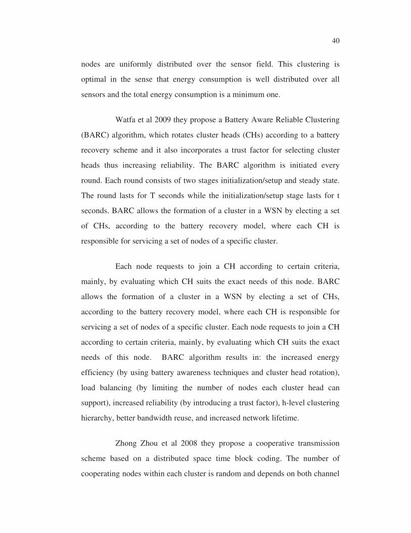
Intuitively, the relationship between coverage and connectivity

depends on the ratio of the communication range to the sensing range.

However, it is easily seen that a connected network may not guarantee its

coverage regardless of the ranges. This is because coverage is concerned with

whether any location is uncovered while connectivity only requires all

locations of active nodes that are connected.

Figure 2.1 Sensing model of sensors

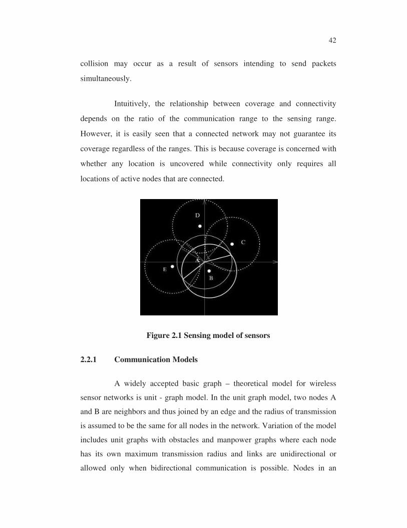
2.2.1 Communication Models

A widely accepted basic graph – theoretical model for wireless

sensor networks is unit - graph model. In the unit graph model, two nodes A

and B are neighbors and thus joined by an edge and the radius of transmission

is assumed to be the same for all nodes in the network. Variation of the model

includes unit graphs with obstacles and manpower graphs where each node

has its own maximum transmission radius and links are unidirectional or

allowed only when bidirectional communication is possible. Nodes in an

43 �

adhoc network may transmit with their maximum transmission radius or may

adjust their transmission range normally selected from a discrete set of

possible values.

The network is normally assumed to be homogeneous; with all

nodes processing the same network attributes such as computational capacity,

battery power and transmission radii. In heterogeneous networks, however

nodes may have different network attributes. In the Random unit graph model

the parameters, are the number of nodes and common transmission radius and

all generated graphs may be either dense or sparse. It is therefore preferable to

use another parameter called average number of neighbors per each node. It is

usually assumed in the literature that each node is aware of its direct

neighbors. In the case that the assumption does not hold a node may broadcast

a “hello” message with all the nodes that receive the message being defined as

neighbors.

2.2.2 Node Category Segregation based on Energy

By calculating the energy of each sensor node the localization is

possible by the formula as given below

� �

Where E is the energy, b is the battery life of each sensor and d is

the amount of data transmitted within the battery life of that sensor.

From the above mentioned formula the energy is individually

calculated for all sensors, to identify the energy level of each sensor. Energy

44 �

level of sensor nodes are divided in 3 ranges which is show in below

Table 2.1.

Table 2.1 Level of Sensors

Range (energy) Level of sensors

Between 0 to 49 Low

Between 50 to 79 Middle

Between 80 to 99 High

This formulation is stated to solve the communication overhead

issue which is described in the following sections.

2.3 LOCALIZING AND OPTIMIZATION OF NODES

The goal of localization is to determine the physical coordinates of

a group of sensor nodes. These coordinates can be global, meaning they are

aligned with some externally meaningful system like GPS, or relative,

meaning that they are an arbitrary “rigid transformation” (rotation, reflection,

translation) away from the global coordinate system. Beacon nodes (also

frequently called anchor nodes) are necessary prerequisite to localizing a

network in a global coordinate system. Beacon nodes are simply ordinary

sensor nodes that know their global coordinates a priori. This knowledge

could be hard coded, or acquired through some additional hardware like GPS

receiver. At a minimum, three non-collinear beacon nodes are required to

define a global coordinate system in two dimensions.

If three dimensional coordinates are required, then at least four non-

coplanar beacons must be present. Beacon nodes can be used in several ways.

Some algorithms like MDSMAP (Yi Shang et al 2003) localize nodes in an

45 �

arbitrary relative coordinate system, then use a few beacon nodes to determine

a rigid transformation of the relative coordinates into global coordinates.

Other algorithms like APIT (He et al 2003) use beacons throughout, using the

positions of several beacons to “bootstrap” the global positions of non-beacon

nodes. Beacon placement can often have a significant impact on localization.

Many groups have found that localization accuracy improves if beacons are

placed in a convex hull around the network. Locating additional beacons in

the center of the network is also helpful.

In any event, there is considerable evidence that real improvements

in localization can be obtained by planning beacon layout in the network. The

advantage of using beacons is obvious: the presence of several pre-localized

nodes can greatly simplify the task of assigning coordinates to ordinary nodes.

However, beacon nodes have inherent disadvantages. GPS receivers are

expensive. They also cannot typically be used indoors, and can also be

confused by tall buildings or other environmental obstacles.

GPS receivers also consume significant battery power, which can

be a problem for power-constrained sensor nodes. The alternative to GPS is

pre-programming nodes with their locations, which can be impractical

(for instance when deploying 10,000 nodes with 500 beacons) or even

impossible (for instance when deploying nodes from an aircraft). In short,

beacons are necessary for localization, but their use does not come without

cost. After estimating the energy of each sensor, all the sensors must be fixed

based on the level of energy (low, middle, high) such that, the higher energy

sensor is considered as the head node for other energy level of sensors.

46 �

2.3.1 Issues in Localization of Sensor Nodes

2.3.1.1 Resource constraints

Sensor networks are typically quite resource-starved. Nodes have

rather weak processors, making large computations infeasible. Moreover,

sensor nodes are typically battery powered. This means communication,

processing, and sensing actions are all expensive, since they actively reduce

the lifespan of the node performing them. Not only that, sensor networks are

typically envisioned on a larger scale, with hundreds or thousands of nodes in

a typical deployment. This fact has two important consequences: nodes must

be cheap to fabricate, and trivially easy to deploy. Nodes must be cheap, since

fifty cents of additional cost per node translates to $500 for one thousand

node network.

Deployment must be easy as well: thirty seconds of handling time

per node to prepare for localization translates to over eight man-hours of work

to deploy 1000 node network. Localization is necessary to many functions of

a sensor network; however, it is not the purpose of a sensor network.

Localization must cost as little as possible while still producing satisfactory

results. That means designers must actively work to minimize the power cost,

hardware cost, and deployment cost of their localization algorithms.

2.3.1.2 Node density

Many localization algorithms are sensitive to node density. For

instance, hop count based schemes generally require high node density so that

the hop count approximation for distance is accurate. Similarly, algorithms

that depend on beacon nodes fail when the beacon density is not high enough

47 �

in a particular region. Thus, when designing or analyzing an algorithm, it is

important to notice the algorithm’s implicit density assumptions, since high

node density can sometimes be expensive if not totally infeasible.

2.3.1.3 Non-convex topologies

Localization algorithms often has trouble positioning nodes near

the edges of a sensor field. This artifact generally occurs because fewer range

measurements are available for border nodes, and those few measurements are

all taken from the same side of the node. In short, border nodes are a problem

because less information is available about them and that information is of

lower quality. This problem is exacerbated, when a sensor network has a non

convex shape: Sensors outside the main convex body of the network can often

prove un-localizable. Even when locations can be found, the results tend to

feature disproportionate error.

2.3.1.4 Environmental obstacles and terrain irregularities

Environmental obstacles and terrain irregularities can also wreak

havoc on localization. Large rocks can occlude line of sight, preventing

TDoA ranging, or interfere with radios, introducing error into RSSI ranges

and producing incorrect hop count ranges. Deployment on grass vs. sand vs.

pavement can affect radios and acoustic ranging systems. Indoors, natural

features like walls can impede measurements as well. All of these issues

are likely to come up in real deployments, so localization systems should be

able to cope.

48 �

2.3.2 FixPos Algorithm

This Position Fixing (Fixpos) algorithm of sensors is used to find

the optimized position in the network. Among the higher energy sensors the

highest energy sensor is chosen as the base node (BN), the remaining higher

energy sensors act as the head node (HN), other middle and low energy

sensors will act as slave nodes (SN).

FixPos algorithm can be explained on the basis of two scenarios:

• Scenario 1 concentrates on the HN and BN where the position

of HN is within the transmission range of BN (Section 4.1.1).

• Scenario 2 concentrates on the SN and HN where the position

of SN is within the transmission range of HN (Section 4.1.2).

2.3.2.1 Fixing the head nodes, BN acts as an actor

The BN is responsible for the communication between all head

nodes, which are placed within the transmission range of BN that is done by

using the expression below (Eq.1). The other energy level of sensors works

within the transmission range of HN.

The position estimate of BN and HN can be found using the

following expression:

[ ] [ ] (2)Rbh(i)(2)rbh(i)↑↑

−−+−− (2.1)

49 �

As shown in the Figure 2.2 ‘R’ denotes the transmission range of

communication of base node ‘b’, ‘r’ denotes the radius. By calculating

(R + r)/2 the head nodes h (i) must be fixed within the dotted circle, which is

the optimized position of the head node represented as

Figure 2.2 Single constraint case

2.3.2.2 Fixing the slave nodes, HN acts as actor

Here, HN is responsible for the communication between all slave

nodes (SN), which are placed within the transmission range of HN that is

done by using the expression below.

The position estimate of SN with respect to HN can be found using

the following expression:

[ ] [ ] 22

Rh(i)srh(i)s −−+−− (2.2)

Where’s denotes the slave nodes.

50 �

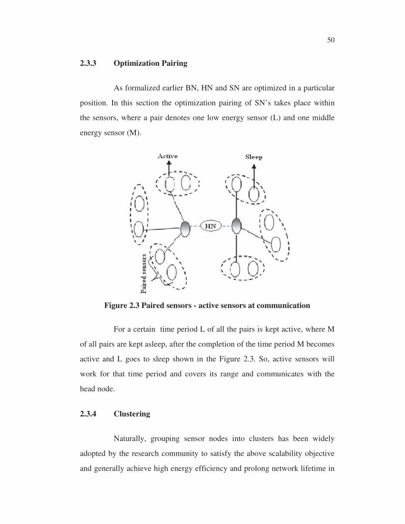
2.3.3 Optimization Pairing

As formalized earlier BN, HN and SN are optimized in a particular

position. In this section the optimization pairing of SN’s takes place within

the sensors, where a pair denotes one low energy sensor (L) and one middle

energy sensor (M).

Figure 2.3 Paired sensors - active sensors at communication

For a certain time period L of all the pairs is kept active, where M

of all pairs are kept asleep, after the completion of the time period M becomes

active and L goes to sleep shown in the Figure 2.3. So, active sensors will

work for that time period and covers its range and communicates with the

head node.

2.3.4 Clustering

Naturally, grouping sensor nodes into clusters has been widely

adopted by the research community to satisfy the above scalability objective

and generally achieve high energy efficiency and prolong network lifetime in

51 �

large-scale WSN environments. The corresponding hierarchical routing and

data gathering protocols imply cluster-based organization of the sensor nodes

in order that data fusion and aggregation are possible, thus leading to

significant energy savings. In the hierarchical network structure each cluster

has a leader, which is also called the cluster head (CH) and usually performs

the special tasks referred above (fusion and aggregation), and several

common sensor nodes (SN) as members.

The cluster formation process eventually leads to a two-level

hierarchy where the CH nodes form the higher level and the cluster-member

nodes form the lower level. The sensor nodes periodically transmit their data

to the corresponding CH nodes. The CH nodes aggregate the data (thus

decreasing the total number of relayed packets) and transmit them to the base

station (BS) either directly or through the intermediate communication with

other CH nodes.

However, because the CH nodes send all the time data to the higher

distances than the common (member) nodes, they naturally spend energy at

higher rates. A common solution in order to balance the energy consumption

among all the network nodes is to periodically re-elect new CHs (thus rotating

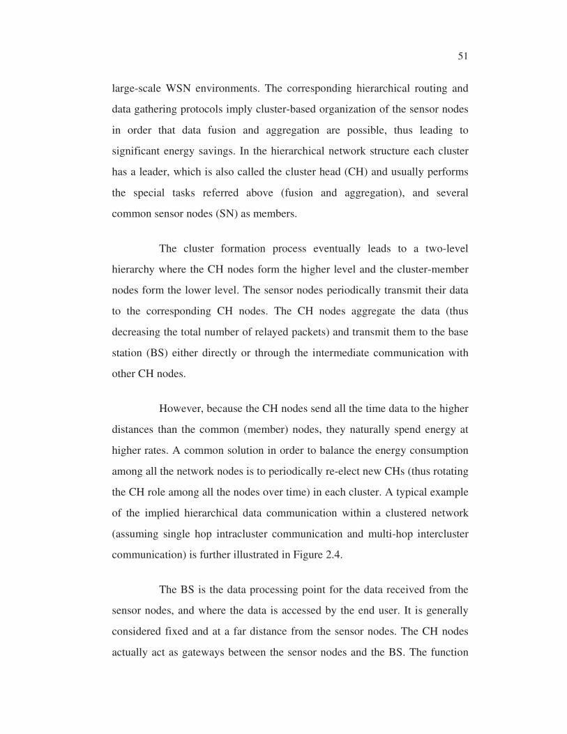
the CH role among all the nodes over time) in each cluster. A typical example

of the implied hierarchical data communication within a clustered network

(assuming single hop intracluster communication and multi-hop intercluster

communication) is further illustrated in Figure 2.4.

The BS is the data processing point for the data received from the

sensor nodes, and where the data is accessed by the end user. It is generally

considered fixed and at a far distance from the sensor nodes. The CH nodes

actually act as gateways between the sensor nodes and the BS. The function

52 �

of each CH, as already mentioned, is to perform common functions for all the

nodes in the cluster, like aggregating the data before sending it to the BS. In

some way, the CH is the sink for the cluster nodes, and the BS is the sink for

the CHs. Moreover, this structure formed between the sensor nodes, the sink

(CH), and the BS can be replicated as many times as it is needed, creating (if

desired) multiple layers of the hierarchical WSN (multi-level cluster

hierarchy).

Figure 2.4 Data communication in a clustered network

In this methodology, clustering uses a hybrid criterion for cluster

formation, which considers the residual energy of each node and a secondary

parameter, such as the node’s proximity to its neighbors or the number of its

neighbors. Clustering plays a great role in reducing the energy consumption

of the nodes, communication overhead and enhancing the network lifetime.

While most of the clustering algorithms focus on the energy balance of the

nodes to prolong the network lifetime, in this research the focus is on

53 �

improving the energy efficiency of the network and to overcome the

communication overhead where the coverage increases automatically.

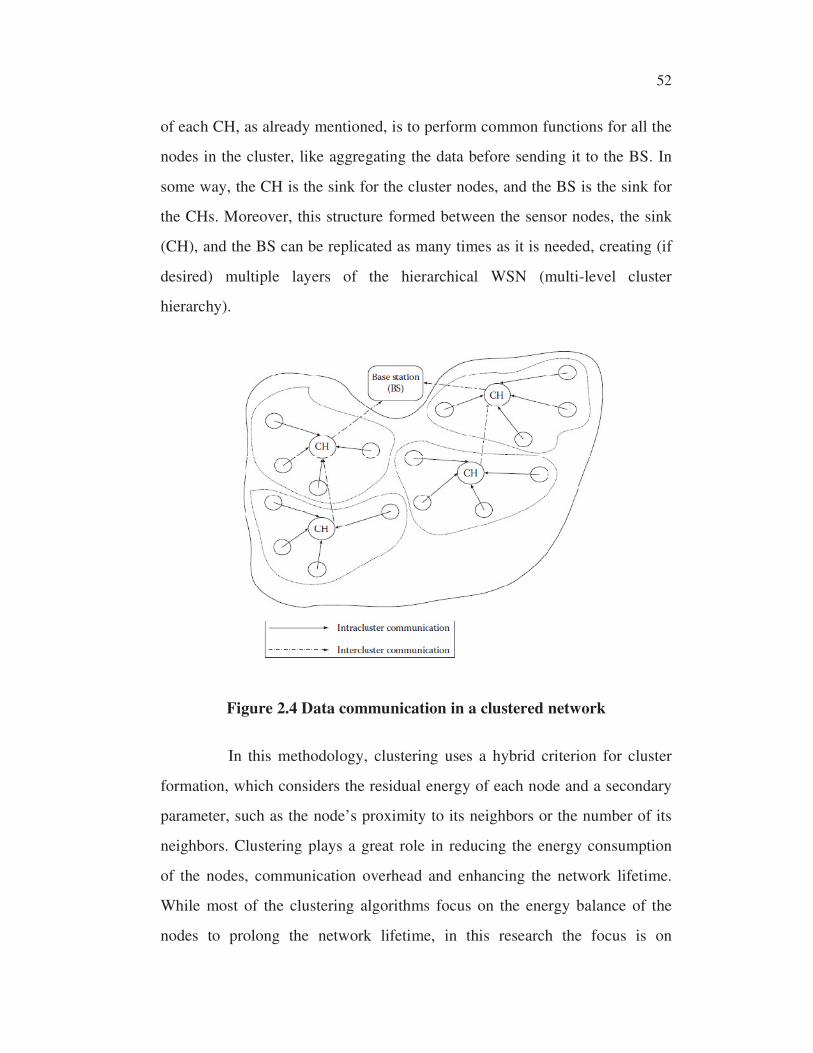
Here a cluster is formed between a HN and certain pair of nodes

such that each cluster is balanced based upon the number of pairs. HN is

mentioned as cluster head. Among the M nodes the adjacent node with

maximum energy in the pair within the cluster is chosen as the back off node

for the cluster head. At any critical situation the primary cluster head is

replaced by the secondary head (back off node).

Figure 2.5 Clustering

The cluster formation of the slave nodes with its head nodes is

shown in the Figure 2.5. In the figure the network is grouped into three

clusters with balanced number of slave nodes for each head nodes. The dotted

circle around the base node is the transmission range where the head nodes

are fixed.

54 �

2.3.5 Distributed Partitioning Connectivity Backup (DPCB)

Algorithm

It’s clear that connectivity only requires the location of any active

node to be within the communication range of one or more active nodes such

that all active nodes can form a connected communication backbone.

Once sensor configuration is finished, nodes shall be comprised of

connected networks to send information collected back to the control center

(Zhu et al 2012).

Inter-node connectivity is not only very crucial to the effectiveness

of the application, but some nodes may also play a role in maintaining flow of

information from the sensors to in situation and remote users.

The failure of a node could hamper the network connectivity and

disrupt the collection of the sensed data. In the worst case, due to a node

failure, the network may get partitioned into multiple disjoint blocks and stop

functioning. Thus, the network connectivity should be recovered so that

subsequent negative effects on the application could be avoided (Tamboli and

Younis 2010).

Rapid restoration of connectivity is desirable in order to maintain

the WSN responsiveness to detected events. Deploying a replacement of the

failed node is a slow solution at best and is often infeasible in risky areas, e.g.,

combat zones. Therefore, the recovery should be a self-healing process

involving the existing nodes. Given the autonomous and unsupervised

operation of WSN, tolerating the failure should be performed in a distributed

manner. In addition, the overhead should be minimized in order to suit the

resource-constrained sensors

55 �

��

��

�� �� ��

��

��

�� �� ��

��

��

�� �� ��

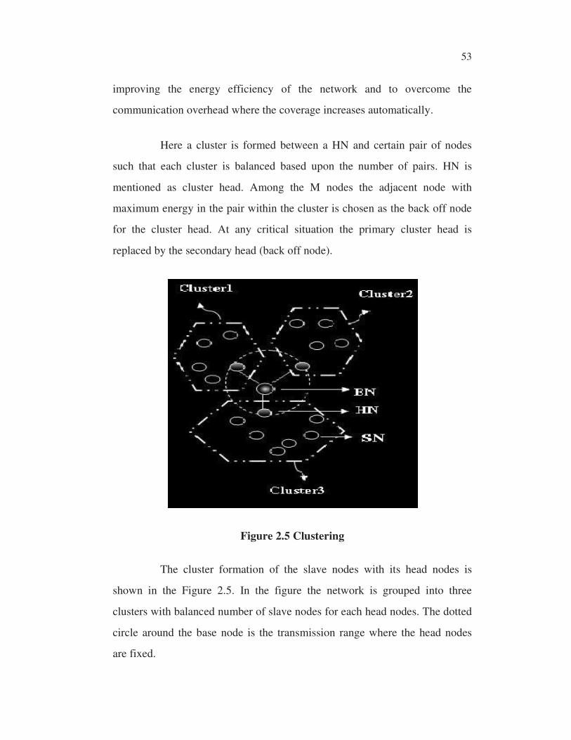
Backup is the procedure for replacing the cluster head when it

meets the critical situation. (Imran et al 2010) the backup node immediately

initiates a recovery process once it detects failure of its primary. The scope of

recovery depends on the position of backup node which can be one of the

following three scenarios.

Figure 2.6(a) Actor b detect the failure of F

Figure 2.6(b) The node B select another nodes us backup

Figure 2.6(c) Moves to the position of F

56 �

��

�� �� ��

Figure 2.6(d) A replacing B and C replacing A

First, if a backup is a non-critical node, the scope of the recovery

will be limited because it does not require further relocations. The backup

node moves to the position of the failed primary and exchange heartbeat

messages with new neighbors. It selects and designates a new backup since it

has become a critical node at the new position. This movement alerts the other

primary nodes (if any) at the previous location to choose a new backup for

themselves.

The second scenario is when the backup is also a critical node. In

this case, the backup node will notify its own backup so that the network stays

connected. This scenario may trigger a series of cascaded repositioning of

nodes. The third scenario is when the failed (primary) and its backup are both

critical nodes and simultaneously serving as backup for each other.

This scenario is articulated in Figure 6 Actor B detects the failure

of F as both are mutually serving as backup for each other as shown in

Figure 2.6(a) and 2.6(b) shows that the node B selects another node’s’ as

backup. Then B sends a movement notification message and moves to the

position of F as shown in Figure 2.6(c). This movement triggers a series of

cascaded relocations as discussed below and is shown in Figure 2.6(d), with A

replacing B and C replacing A.

57 �

2.3.6 Performance Evaluation

2.3.6.1 Simulation parameters

The proposed scheme is evaluated through NS2 simulation. The

bounded region of 1000 x 1000 sq.m is used, in which nodes are placed in a

uniform distribution. The power levels of the nodes are assigned such that the

transmission range and the sensing range of the nodes are all 250 meters. In

the simulation, the channel capacity of mobile hosts is set to the same value: 2

Mbps. The distributed coordination function (DCF) of IEEE 802.11 is used

for wireless LANs as the MAC layer protocol. It has the functionality to

notify the network layer about link breakage. In the simulation, sensor nodes

of 200 are deployed in a 1000 m x 1000 m rectangular region for 50 seconds

of simulation time.

The simulated traffic is Constant Bit Rate (CBR). To measure the

performance of different protocols under different ratios of communication

range/sensing range, the communication range is varied by 250,300,350 and

450m, in the network interface. All experimental results presented in this

section are averages of five runs on different randomly chosen scenarios. The

following Table 2.2 summarizes the simulation parameters used.

�

58 �

Table 2.2 Simulation parameters

No. of Nodes 200

Area Size 1000 X 1000

Mac 802.11

Simulation Time 50 sec

Traffic Source CBR

Packet Size 512

Transmit Power 0.360 w

Receiving Power 0.395 w

Idle Power 0.335 w

Transmission Range 250,300,350 and 400

Routing Protocol AODV

In the simulations, the following metrics were used to evaluate the

performance: (i) energy efficiency; (ii) average size of the clusters;

(iii) sensors lifetime.

2.3.6.2 Simulation background

Most of the algorithms perform simulations using Matlab and Ns2,

the proposed algorithm is evaluated using Ns2.

Ns2 stands for network simulator which is an object-oriented,

discrete event driven network simulator developed at UC Berkeley. Ns2 is a

commonly used tool to simulate the behavior of wired and wireless networks.

Ns provides significant support for simulation of TCP, routing, and multicast

protocols over wired and wireless (local and satellite) networks. It also

59 �

supports applications like web caching too. And also it implements network

protocols such as TCP and UDP, traffic source behavior such as FTP, Telnet,

Web, CBR and VBR, router queue management mechanism such as Drop

Tail, RED and CBQ, routing algorithms. As well Ns2 implements

multicasting and some of the MAC layer protocols for LAN simulations.

Ns2 Simulator is based on two languages: an object oriented

Simulator, written in C++, and an OTcl (an object oriented extension of Tcl

(Tool Command Language)) interpreter, used to execute user’s command

scripts. The simulator is based on two class hierarchies: the compiled C++

hierarchy and the interpreted OTcl one, with one to one correspondence

between them. There are two specifications that have to be achieved by the

simulator, so these two languages are used by ns. Detailed simulations of

protocols need a systems programming language which can competently

manipulate bytes, packet headers, and implement algorithms.

The compiled C++ hierarchy achieves efficiency in the simulation

and faster execution times, and reduces packet and event processing time. In

the OTcl script provided by user the particular network topology, the specific

protocols, the applications which will be simulated, and the form of the output

can be defined. The OTcl can make use of objects compiled in C++ through

an OTcl linkage that creates a matching of OTcl object for each of the C++.

The code to interface with the OTcl interpreter resides in a separate directory,

tclcl. The rest of the simulator code resides in the Ns2 directory.

The most important six classes that are used in Ns2: The Class Tcl,

containing the methods that C++ code will use to access the interpreter, the

class TclObject, the base class for all simulator objects that are also mirrored

in the compiled hierarchy. The class TclClass, defining the interpreted class

60 �

hierarchy, and the methods to permit the user to instantiate TclObjects, the

class TclCommand, used to define simple global interpreter commands, the

class EmbeddedTcl containing the methods to load higher level built-in

commands that make configuring simulations easier, and the class InstVar

containing methods to Access C++ member variables as OTcl instance

variables.

Ns2 includes a tool for viewing the simulation results, called Nam,

the network animator. Nam is a Tcl/Tk based animation tool to visualize the

network simulation traces and real world packet trace data. The design theory

behind nam is to create an animator that is able to read large animation data

sets and be extensible enough so that it could be used in different network

visualization situations. Under this constraint nam is designed to read simple

animation event commands from a large trace file. In order to handle large

animation data sets a minimum amount of information is kept in memory.

Event commands are kept in the file and re-read from the file whenever

necessary.

To sum up ns is an object-oriented, discrete event driven network

simulator. Since ns is an extensible and an open source program, it is suitable

for academic and educational purposes. Moreover it is possible to create new

algorithms using a rich library of network and protocol objects.

2.3.6.3 Energy efficiency

It is assumed that the BN has two level transmission power with the

transmission radii � and �= 2�, respectively. First, 100 sensor nodes are

deployed randomly and the transmission radius � is set to 15 meters. For

example, when n = 100 and the battery/network lifetime ratio is�

. Both

61 �

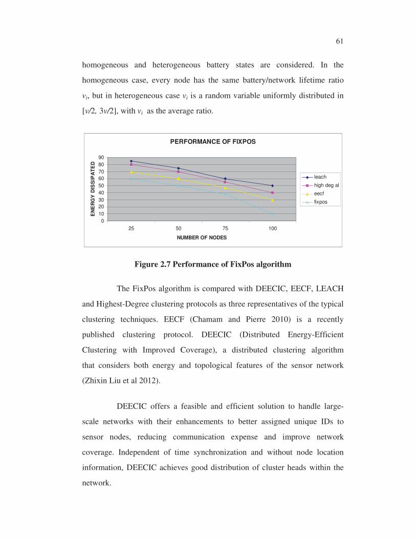
homogeneous and heterogeneous battery states are considered. In the

homogeneous case, every node has the same battery/network lifetime ratio

vi, but in heterogeneous case vi is a random variable uniformly distributed in

[v/2, 3v/2], with vi as the average ratio.

Figure 2.7 Performance of FixPos algorithm

The FixPos algorithm is compared with DEECIC, EECF, LEACH

and Highest-Degree clustering protocols as three representatives of the typical

clustering techniques. EECF (Chamam and Pierre 2010) is a recently

published clustering protocol. DEECIC (Distributed Energy-Efficient

Clustering with Improved Coverage), a distributed clustering algorithm

that considers both energy and topological features of the sensor network

(Zhixin Liu et al 2012).

DEECIC offers a feasible and efficient solution to handle large-

scale networks with their enhancements to better assigned unique IDs to

sensor nodes, reducing communication expense and improve network

coverage. Independent of time synchronization and without node location

information, DEECIC achieves good distribution of cluster heads within the

network.

PERFORMANCE OF FIXPOS

0

10

20

30

40

50

60

70

80

90

25 50 75 100

NUMBER OF NODES

EN

ER

GY

DIS

SIP

AT

ED

leach

high deg al

eecf

fixpos

62 �

DEECIC is also a fast and locally scalable: since sensor nodes are

energy-constrained, frequently receiving data from common nodes and

forwarding them to the base station will consume a large amount of energy on

cluster heads, DEECIC can achieve re-clustering within constant time and in a

local manner. In EECF, a sensor’s eligibility to be elected as cluster head is

based on its residual energy and its degree. However, cluster heads also act as

data relays, since they route received data from peer cluster heads toward the

base station, either directly if the base station is within their transmitting

ranges or through a neighboring cluster head if the base station is beyond

transmitting range. LEACH (Chandrakasan et al 2004) was proposed for an

application in which nodes are randomly distributed in a square area.

In LEACH, nodes continuously sense the environment, and then

send data packets to the base station. LEACH rotates the cluster heads in

every round, with an aim at prolonging the network lifetime. Similarly to

proposed scheme, the Highest-Degree algorithm (Gerla and Tsai 1995) known

as connectivity-based clustering, selects the nodes with the maximum number

of neighbors as cluster heads. Note that all the tested clustering algorithms use

the same parameters in each simulation.

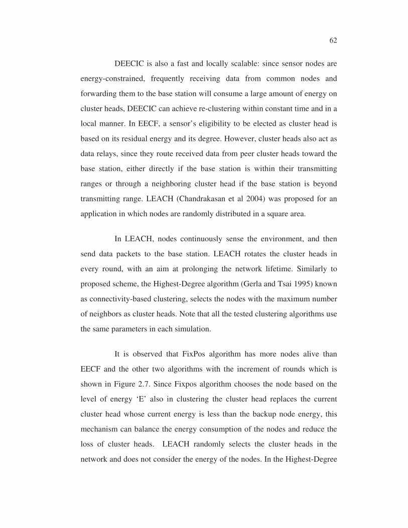
It is observed that FixPos algorithm has more nodes alive than

EECF and the other two algorithms with the increment of rounds which is

shown in Figure 2.7. Since Fixpos algorithm chooses the node based on the

level of energy ‘E’ also in clustering the cluster head replaces the current

cluster head whose current energy is less than the backup node energy, this

mechanism can balance the energy consumption of the nodes and reduce the

loss of cluster heads. LEACH randomly selects the cluster heads in the

network and does not consider the energy of the nodes. In the Highest-Degree

63 �

algorithm, once a cluster head is selected, it continues to relay data until the

energy is used up, which may result in faster death of some nodes.

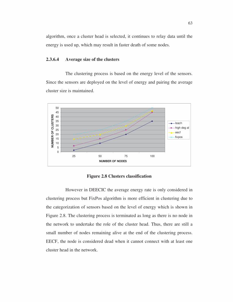
2.3.6.4 Average size of the clusters

The clustering process is based on the energy level of the sensors.

Since the sensors are deployed on the level of energy and pairing the average

cluster size is maintained.

Figure 2.8 Clusters classification

However in DEECIC the average energy rate is only considered in

clustering process but FixPos algorithm is more efficient in clustering due to

the categorization of sensors based on the level of energy which is shown in

Figure 2.8. The clustering process is terminated as long as there is no node in

the network to undertake the role of the cluster head. Thus, there are still a

small number of nodes remaining alive at the end of the clustering process.

EECF, the node is considered dead when it cannot connect with at least one

cluster head in the network.

0

5

10

15

20

25

30

35

40

45

50

25 50 75 100

NUMBER OF NODES

NU

MB

ER

OF

CL

US

TE

RS

leach

high deg al

eecf

fixpos

64 �

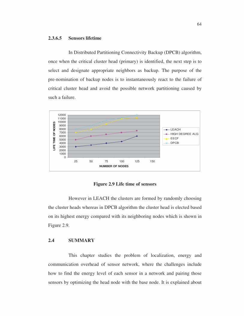
2.3.6.5 Sensors lifetime

In Distributed Partitioning Connectivity Backup (DPCB) algorithm,

once when the critical cluster head (primary) is identified, the next step is to

select and designate appropriate neighbors as backup. The purpose of the

pre-nomination of backup nodes is to instantaneously react to the failure of

critical cluster head and avoid the possible network partitioning caused by

such a failure.

Figure 2.9 Life time of sensors

However in LEACH the clusters are formed by randomly choosing

the cluster heads whereas in DPCB algorithm the cluster head is elected based

on its highest energy compared with its neighboring nodes which is shown in

Figure 2.9.

2.4 SUMMARY

This chapter studies the problem of localization, energy and

communication overhead of sensor network, where the challenges include

how to find the energy level of each sensor in a network and pairing those

sensors by optimizing the head node with the base node. It is explained about

0

1000

2000

3000

4000

5000

6000

7000

8000

9000

10000

11000

12000

25 50 75 100 125 150

NUMBER OF NODES

LIF

E T

IME

OF

NO

DE

S

LEACH

HIGH DEGREE ALG

EECF

DPCB

65 �

the active nodes and sleep nodes state where the scope of each node is

responsible for increasing the lifetime of the network. It is examined the

formation of clusters with balancing number of slave nodes in each cluster.

The optimal cluster size is maintained to minimize the average energy

consumption rate per unit area for a network. The proposed DPCB algorithm

uses a back off strategy which is used to minimize the communication

overhead issue that simultaneously increases the network coverage. Various

scenarios are presented to show the scope of recovery which depends on the

position of the backup node. Our simulation results validate this computation,

and show the improvement of overcoming the communication overhead.