Embed Size (px)
Citation preview
Introduction Discrete distributions Life distributions
Chapter 2Failure Models – Part 1
Marvin [email protected]
RAMS GroupDepartment of Production and �ality Engineering
NTNU
(Version 0.1)
Marvin Rausand (RAMS Group) System Reliability Theory (Version 0.1) 1 / 36
Introduction Discrete distributions Life distributions
Slides related to the book
System Reliability TheoryModels, Statistical Methods,and Applications
Wiley, 2004
Homepage of the book:http://www.ntnu.edu/ross/books/srt
Marvin Rausand (RAMS Group) System Reliability Theory (Version 0.1) 2 / 36
Introduction Discrete distributions Life distributions
Objectives
This presentation will introduce:I Reliability measures for non-repaired items:
• The reliability (survivor) function R(t)• The failure rate function z(t)• The mean time to failure (MTTF)• The mean residual life (MRL)
I Some common discrete distributions:• The binomial distribution• The geometric distribution• The Poisson distribution – and the Poisson process
I Some common life distributions:• The Exponential distribution• The Weibull distribution
Marvin Rausand (RAMS Group) System Reliability Theory (Version 0.1) 3 / 36
Introduction Discrete distributions Life distributions
Reliability measures
Here, we only consider an item that is not repaired. The item may berepairable, but we only consider it until the first failure.
Before introducing the reliability measures, we have to define the twoconcepts:I State variableI Time to failure
Marvin Rausand (RAMS Group) System Reliability Theory (Version 0.1) 4 / 36
Introduction Discrete distributions Life distributions
State variable
X(t)
0t
1
Time to failure, T
Failure
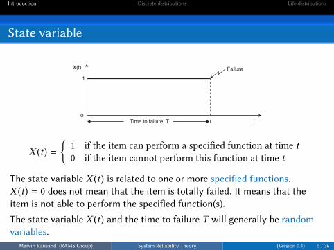
X (t) ={
1 if the item can perform a speci�ed function at time t0 if the item cannot perform this function at time t
The state variable X (t) is related to one or more specified functions.X (t) = 0 does not mean that the item is totally failed. It means that theitem is not able to perform the specified function(s).
The state variable X (t) and the time to failure T will generally be randomvariables.
Marvin Rausand (RAMS Group) System Reliability Theory (Version 0.1) 5 / 36

Introduction Discrete distributions Life distributions
Item
We use the term item to denote any physical component, assembly, orsystem.
In some applications, the item may be a small component, while it in otherapplications may be a large system.
Marvin Rausand (RAMS Group) System Reliability Theory (Version 0.1) 6 / 36
Introduction Discrete distributions Life distributions
Time to failure
The time to failure can be measured by di�erent time concepts
I Calendar timeI Operational timeI Number of kilometers driven by a carI Number of cycles for a periodically working itemI Number of times a switch is operatedI Number of rotations of a bearing
In most applications, we assume that the time to failure T is a continuousrandom variable (Discrete variables may be approximated by a continuousvariable)
Marvin Rausand (RAMS Group) System Reliability Theory (Version 0.1) 7 / 36
Introduction Discrete distributions Life distributions
Probability distribution function
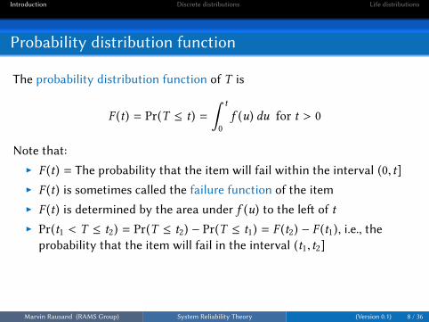
The probability distribution function of T is
F (t) = Pr(T ≤ t) =∫ t
0f (u) du for t > 0
Note that:I F (t) = The probability that the item will fail within the interval (0, t]I F (t) is sometimes called the failure function of the itemI F (t) is determined by the area under f (u) to the le� of tI Pr(t1 < T ≤ t2) = Pr(T ≤ t2) − Pr(T ≤ t1) = F (t2) − F (t1), i.e., the
probability that the item will fail in the interval (t1, t2]
Marvin Rausand (RAMS Group) System Reliability Theory (Version 0.1) 8 / 36
Introduction Discrete distributions Life distributions
Probability density function
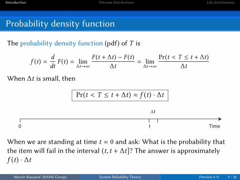
The probability density function (pdf) of T is
f (t) =ddt
F (t) = lim∆t→∞
F (t + ∆t) − F (t)∆t
= lim∆t→∞
Pr(t < T ≤ t + ∆t)∆t
When ∆t is small, then
Pr(t < T ≤ t + ∆t) ≈ f (t) · ∆t
0 t
Δ t
Time
When we are standing at time t = 0 and ask: What is the probability thatthe item will fail in the interval (t, t + ∆t]? The answer is approximatelyf (t) · ∆t
Marvin Rausand (RAMS Group) System Reliability Theory (Version 0.1) 9 / 36
Introduction Discrete distributions Life distributions
Distribution of T
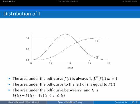
I The area under the pdf-curve f (t) is always 1,∫ ∞
0 f (t) dt = 1I The area under the pdf-curve to the le� of t is equal to F (t)I The area under the pdf-curve between t1 and t2 isF (t2) − F (t1) = Pr(t1 < T ≤ t2)
Marvin Rausand (RAMS Group) System Reliability Theory (Version 0.1) 10 / 36
Introduction Discrete distributions Life distributions
Survivor function
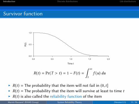
R(t) = Pr(T > t) = 1 − F (t) =∫ ∞
tf (u) du
I R(t) = The probability that the item will not fail in (0, t]I R(t) = The probability that the item will survive at least to time tI R(t) is also called the reliability function of the itemMarvin Rausand (RAMS Group) System Reliability Theory (Version 0.1) 11 / 36
Introduction Discrete distributions Life distributions
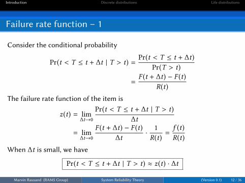
Failure rate function – 1
Consider the conditional probability
Pr(t < T ≤ t + ∆t | T > t) =Pr(t < T ≤ t + ∆t)
Pr(T > t)
=F (t + ∆t) − F (t)
R(t)
The failure rate function of the item is
z(t) = lim∆t→0
Pr(t < T ≤ t + ∆t | T > t)∆t
= lim∆t→0
F (t + ∆t) − F (t)∆t
·1
R(t)=
f (t)R(t)
When ∆t is small, we have
Pr(t < T ≤ t + ∆t | T > t) ≈ z(t) · ∆t
Marvin Rausand (RAMS Group) System Reliability Theory (Version 0.1) 12 / 36
Introduction Discrete distributions Life distributions
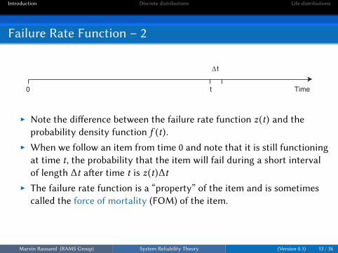
Failure Rate Function – 2
0 t
Δ t
Time
I Note the di�erence between the failure rate function z(t) and theprobability density function f (t).
I When we follow an item from time 0 and note that it is still functioningat time t, the probability that the item will fail during a short intervalof length ∆t a�er time t is z(t)∆t
I The failure rate function is a “property” of the item and is sometimescalled the force of mortality (FOM) of the item.
Marvin Rausand (RAMS Group) System Reliability Theory (Version 0.1) 13 / 36
Introduction Discrete distributions Life distributions
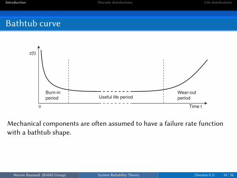
Bathtub curve
z(t)
Time t0
Burn-inperiod Useful life period
Wear-outperiod
Mechanical components are o�en assumed to have a failure rate functionwith a bathtub shape.
Marvin Rausand (RAMS Group) System Reliability Theory (Version 0.1) 14 / 36
Introduction Discrete distributions Life distributions
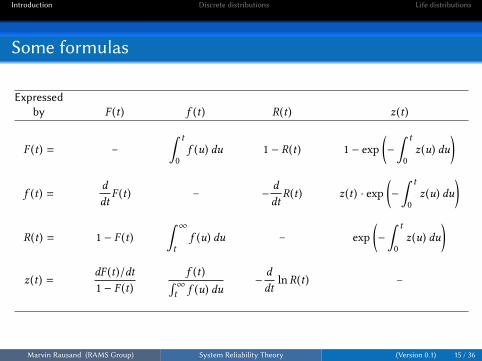
Some formulas
Expressedby F (t) f (t) R(t) z(t)
F (t) = –∫ t
0f (u) du 1 − R(t) 1 − exp
(−
∫ t
0z(u) du
)
f (t) =ddtF (t) – −
ddtR(t) z(t) · exp
(−
∫ t
0z(u) du
)
R(t) = 1 − F (t)∫ ∞t
f (u) du – exp(−
∫ t
0z(u) du
)
z(t) =dF (t)/dt1 − F (t)
f (t)∫ ∞t f (u) du
−ddt
ln R(t) –
Marvin Rausand (RAMS Group) System Reliability Theory (Version 0.1) 15 / 36
Introduction Discrete distributions Life distributions
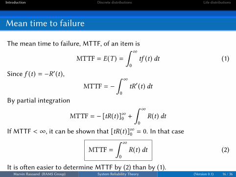
Mean time to failure
The mean time to failure, MTTF, of an item is
MTTF = E(T ) =∫ ∞
0tf (t) dt (1)
Since f (t) = −R′(t),
MTTF = −∫ ∞
0tR′(t) dt
By partial integration
MTTF = − [tR(t)]∞0 +∫ ∞
0R(t) dt
If MTTF < ∞, it can be shown that [tR(t)]∞0 = 0. In that case
MTTF =∫ ∞
0R(t) dt (2)
It is o�en easier to determine MTTF by (2) than by (1).Marvin Rausand (RAMS Group) System Reliability Theory (Version 0.1) 16 / 36
Introduction Discrete distributions Life distributions
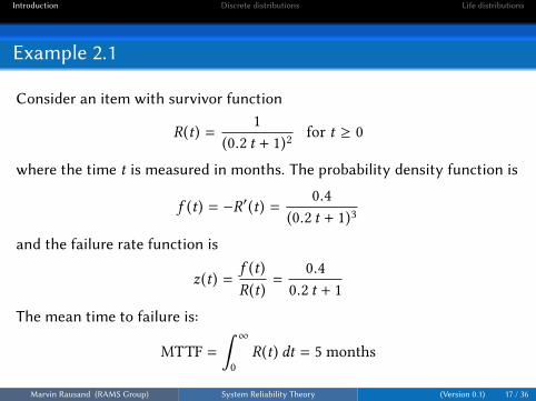
Example 2.1
Consider an item with survivor function
R(t) =1
(0.2 t + 1)2for t ≥ 0
where the time t is measured in months. The probability density function is
f (t) = −R′(t) =0.4
(0.2 t + 1)3
and the failure rate function is
z(t) =f (t)R(t)
=0.4
0.2 t + 1
The mean time to failure is:
MTTF =∫ ∞
0R(t) dt = 5 months
Marvin Rausand (RAMS Group) System Reliability Theory (Version 0.1) 17 / 36
Introduction Discrete distributions Life distributions
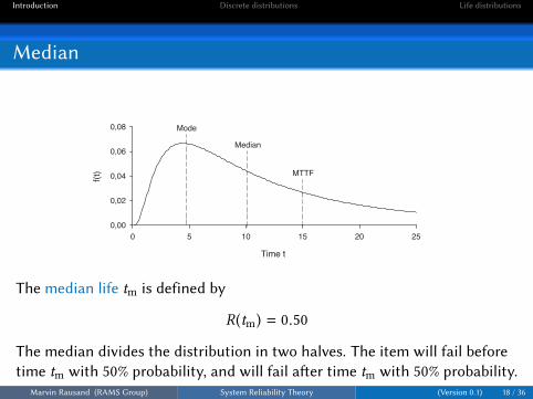
Median
Time t
0 5 10 15 20 25
f(t)
0,00
0,02
0,04
0,06
0,08 Mode
Median
MTTF
The median life tm is defined by
R(tm) = 0.50
The median divides the distribution in two halves. The item will fail beforetime tm with 50% probability, and will fail a�er time tm with 50% probability.
Marvin Rausand (RAMS Group) System Reliability Theory (Version 0.1) 18 / 36
Introduction Discrete distributions Life distributions
Mode
The mode of a life distribution is the most likely failure time, that is, thetime tmode where the probability density function f (t) a�ains its maximum(see figure on the previous slide).
Marvin Rausand (RAMS Group) System Reliability Theory (Version 0.1) 19 / 36
Introduction Discrete distributions Life distributions
Conditional survivor function
Consider an item that is put into operation at time t = 0 and is stillfunctioning at time t. The probability that the item of age t survives anadditional interval of length x is
R(x | t) = Pr(T > x + t | T > t) =Pr(T > x + t)
Pr(T > t)=
R(x + t)R(t)
R(x | t) is called the conditional survivor function of the item at age t.
With this notationR(x | 0) = R(x)
Marvin Rausand (RAMS Group) System Reliability Theory (Version 0.1) 20 / 36
Introduction Discrete distributions Life distributions
Mean residual life
The mean residual life, MRL(t), of the item at age t is
MRL(t) = µ (t) =∫ ∞
0R(x | t) dx =
1R(t)
∫ ∞
tR(x) dx
I MRL is also called the mean remaining lifeI MRL(0) of a new item may, for example, be 15 000 hours. When the
item is still functioning a�er 10 000 hours, its MRL(10 000 hours) may,for example, be 8 000 hours. Note that generally MRL(x) ,MRL(0) − x
I When we determine MRL(x) we know (or assume) that the item isfunctioning at time x, but we do not have any additional informationabout what happened in the interval (0,x)
Marvin Rausand (RAMS Group) System Reliability Theory (Version 0.1) 21 / 36
Introduction Discrete distributions Life distributions
Example 2.2 – 1
Consider an item with failure rate function z(t) = t/(t + 1). The failure ratefunction is increasing and approaches 1 when t → ∞. The correspondingsurvivor function is
R(t) = exp(−
∫ t
0
uu + 1
du)= (t + 1) e−t
MTTF =∫ ∞
0(t + 1) e−t dt = 2
The conditional survival function is
R(x | t) = Pr(T > x + t | T > t) =(t + x + 1) e−(t+x)
(t + 1) e−t=
t + x + 1t + 1
e−x
Marvin Rausand (RAMS Group) System Reliability Theory (Version 0.1) 22 / 36
Introduction Discrete distributions Life distributions
Example 2.2 – 2
The mean residual life is
MRL(t) =∫ ∞
0R(x | t) dx = 1 +
1t + 1
We see that MRL(t) is equal to 2 (= MTTF) when t = 0, that MRL(t) is adecreasing function in t, and that MRL(t) → 1 when t → ∞.
Marvin Rausand (RAMS Group) System Reliability Theory (Version 0.1) 23 / 36

Introduction Discrete distributions Life distributions
Discrete distributions
Three discrete distributions are introduced:
I The binomial distributionI The geometric distributionI The Poisson distribution – incl. the homogeneous Poisson process
Marvin Rausand (RAMS Group) System Reliability Theory (Version 0.1) 24 / 36
Introduction Discrete distributions Life distributions
Binomial distribution – 1
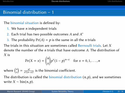
The binomial situation is defined by:
1. We have n independent trials
2. Each trial has two possible outcomes A and A∗
3. The probability Pr(A) = p is the same in all the n trials
The trials in this situation are sometimes called Bernoulli trials. Let Xdenote the number of the n trials that have outcome A. The distribution ofX is
Pr(X = x) =(nx
)px (1 − p)n−x for x = 0,1, . . . ,n
where(nx
)= n!
x!(n−x)! is the binomial coe�icient.
The distribution is called the binomial distribution (n,p), and we sometimeswrite X ∼ bin(n,p).
Marvin Rausand (RAMS Group) System Reliability Theory (Version 0.1) 25 / 36
Introduction Discrete distributions Life distributions
Binomial distribution – 2
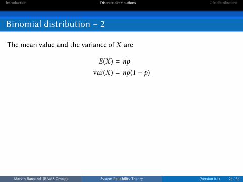
The mean value and the variance of X are
E(X ) = np
var(X ) = np(1 − p)
Marvin Rausand (RAMS Group) System Reliability Theory (Version 0.1) 26 / 36

Introduction Discrete distributions Life distributions
Geometric distribution – 1
Assume that we carry out a sequence of Bernoulli trials, and want to findthe number Z of trials until the first trial with outcome A. If Z = z, thismeans that the first (z − 1) trials have outcome A∗, and that the first A willoccur in trial z. The distribution of Z is
Pr(Z = z) = (1 − p)z−1p for z = 1,2, . . .
This distribution is called the geometric distribution. We have that
Pr(Z > z) = (1 − p)z
Marvin Rausand (RAMS Group) System Reliability Theory (Version 0.1) 27 / 36
Introduction Discrete distributions Life distributions
Geometric distribution – 2
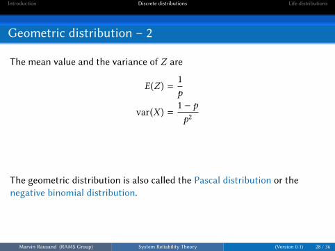
The mean value and the variance of Z are
E(Z ) =1p
var(X ) =1 − pp2
The geometric distribution is also called the Pascal distribution or thenegative binomial distribution.
Marvin Rausand (RAMS Group) System Reliability Theory (Version 0.1) 28 / 36
Introduction Discrete distributions Life distributions
The homogeneous Poisson process –1
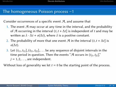
Consider occurrences of a specific event A, and assume that
1. The event A may occur at any time in the interval, and the probabilityofA occurring in the interval (t, t + ∆t] is independent of t and may bewri�en as λ · ∆t + o(∆t), where λ is a positive constant.
2. The probability of more that one event A in the interval (t, t + ∆t] iso(∆t).
3. Let (t11, t12], (t21, t22], . . . be any sequence of disjoint intervals in thetime period in question. Then the events “A occurs in (tj1, tj2],”j = 1,2, . . ., are independent.
Without loss of generality we let t = 0 be the starting point of the process.
Marvin Rausand (RAMS Group) System Reliability Theory (Version 0.1) 29 / 36
Introduction Discrete distributions Life distributions
The homogeneous Poisson process – 2
Let N (t) denote the number of times the event A occurs during the interval(0, t]. The stochastic process {N (t), t ≥ 0} is called a Homogeneous PoissonProcess (HPP) with rate λ.
The distribution of N (t) is
Pr(N (t) = n) =(λt)n
n!e−λt for n = 0,1,2, . . .
The mean and the variance of N (t) are
E(N (t)) =∞∑n=0
n · Pr(N (t) = n) = λt
var(N (t)) = λt
Marvin Rausand (RAMS Group) System Reliability Theory (Version 0.1) 30 / 36

Introduction Discrete distributions Life distributions
Life distributions
Only two life distributions are introduced:
I The exponential distributionI The Weibull distribution (with two parameters)
Several more life distributions are covered in the book.
Marvin Rausand (RAMS Group) System Reliability Theory (Version 0.1) 31 / 36
Introduction Discrete distributions Life distributions
Exponential distribution – 1
Consider an item that is put into operation at time t = 0. Assume that thetime to failure T of the item has probability density function (pdf)
f (t) ={
λe−λt for t > 0, λ > 00 otherwise
This distribution is called the exponential distribution with parameter λ,and we sometimes write T ∼ exp(λ).The survivor function of the item is
R(t) = Pr(T > t) =∫ ∞
tf (u) du = e−λt for t > 0
The mean and the variance of T are
MTTF =∫ ∞
0R(t) dt =
∫ ∞
0e−λt dt =
1λ
var(T ) = 1/λ2
Marvin Rausand (RAMS Group) System Reliability Theory (Version 0.1) 32 / 36
Introduction Discrete distributions Life distributions
Exponential distribution – 2
The failure rate function is
z(t) =f (t)R(t)
=λe−λt
e−λt= λ
The failure rate function is hence constant and independent of time.Consider the conditional survivor function
R(x | t) = Pr(T > t + x | T > t) =Pr(T > t + x)
Pr(T > t)
=e−λ (t+x)
e−λt= e−λx = Pr(T > x) = R(x)
A new item, and a used item (that is still functioning), will therefore havethe same probability of surviving a time interval of length t.A used item is therefore stochastically as-good-as-new.
Marvin Rausand (RAMS Group) System Reliability Theory (Version 0.1) 33 / 36
Introduction Discrete distributions Life distributions
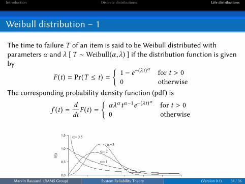
Weibull distribution – 1
The time to failure T of an item is said to be Weibull distributed withparameters α and λ [ T ∼Weibull(α ,λ) ] if the distribution function is givenby
F (t) = Pr(T ≤ t) ={
1 − e−(λt)α for t > 00 otherwise
The corresponding probability density function (pdf) is
f (t) =ddtF (t) =
{αλα tα−1e−(λt)
α for t > 00 otherwise
Time t
0,0 0,5 1,0 1,5 2,0 2,5 3,0
f(t)
0,0
0,5
1,0
1,5 α = 0.5
α = 1
α = 2
α = 3
Marvin Rausand (RAMS Group) System Reliability Theory (Version 0.1) 34 / 36
Introduction Discrete distributions Life distributions
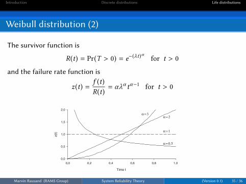
Weibull distribution (2)
The survivor function is
R(t) = Pr(T > 0) = e−(λt)α
for t > 0
and the failure rate function is
z(t) =f (t)R(t)
= αλα tα−1 for t > 0
Time t
0,0 0,2 0,4 0,6 0,8 1,0
z(t)
0,0
0,5
1,0
1,5
2,0
α = 0.5
α = 1
α = 2α = 3
Marvin Rausand (RAMS Group) System Reliability Theory (Version 0.1) 35 / 36
Introduction Discrete distributions Life distributions
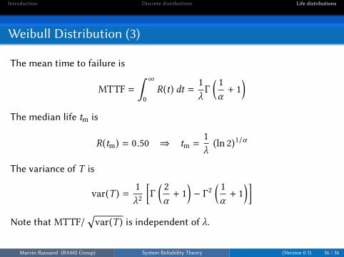
Weibull Distribution (3)
The mean time to failure is
MTTF =∫ ∞
0R(t) dt =
1λΓ
( 1α+ 1
)The median life tm is
R(tm) = 0.50 ⇒ tm =1λ(ln 2)1/α
The variance of T is
var(T ) =1λ2
[Γ
( 2α+ 1
)− Γ2
( 1α+ 1
)]Note that MTTF/
√var(T ) is independent of λ.
Marvin Rausand (RAMS Group) System Reliability Theory (Version 0.1) 36 / 36