Embed Size (px)
Citation preview
CHAPTER 2
First Order Equations
IN THIS CHAPTER we study first order equations for which there are general methods of solution.
SECTION 2.1 deals with linear equations, the simplest kind of first order equations. In this section weintroduce the method of variation of parameters. The idea underlying this method will be a unifyingtheme for our approach to solving many different kinds of differential equations throughout the book.
SECTION 2.2 deals with separable equations, the simplest nonlinear equations. In this section we intro-duce the idea of implicit and constant solutions of differential equations, and we point out some differ-ences between the properties of linear and nonlinear equations.
SECTION 2.3 discusses existence and uniqueness of solutions of nonlinear equations. Although it mayseem logical to place this section before Section 2.2, we presented Section 2.2 first so we could haveillustrative examples in Section 2.3.
SECTION 2.4 deals with nonlinear equations that are not separable, but can be transformed into separableequations by a procedure similar to variation of parameters.
SECTION 2.5 covers exact differential equations, which are given this name because the method forsolving them uses the idea of an exact differential from calculus.
SECTION 2.6 deals with equations that are not exact, but can made exact by multiplying them by afunction known called integrating factor.
29

30 Chapter 2 First Order Equations
2.1 LINEAR FIRST ORDER EQUATIONS
A first order differential equation is said to be linear if it can be written as
y0 C p.x/y D f .x/: (2.1.1)
A first order differential equation that can’t be written like this is nonlinear. We say that (2.1.1) ishomogeneous if f ! 0; otherwise it’s nonhomogeneous. Since y ! 0 is obviously a solution of thehomgeneous equation
y0 C p.x/y D 0;
we call it the trivial solution. Any other solution is nontrivial.
Example 2.1.1 The first order equations
x2y0 C 3y D x2;
xy0 " 8x2y D sinx;
xy0 C .lnx/y D 0;
y0 D x2y " 2;
are not in the form (2.1.1), but they are linear, since they can be rewritten as
y0 C3
x2y D 1;
y0 " 8xy Dsin x
x;
y0 Clnx
xy D 0;
y0 " x2y D "2:
Example 2.1.2 Here are some nonlinear first order equations:
xy0 C 3y2 D 2x (because y is squared);
yy0 D 3 (because of the product yy0);
y0 C xey D 12 (because of ey):
General Solution of a Linear First Order Equation
To motivate a definition that we’ll need, consider the simple linear first order equation
y0 D1
x2: (2.1.2)
From calculus we know that y satisfies this equation if and only if
y D "1
xC c; (2.1.3)
where c is an arbitrary constant. We call c a parameter and say that (2.1.3) defines a one–parameterfamily of functions. For each real number c, the function defined by (2.1.3) is a solution of (2.1.2) on
Section 2.1 Linear First Order Equations 31
.!1; 0/ and .0;1/; moreover, every solution of (2.1.2) on either of these intervals is of the form (2.1.3)for some choice of c. We say that (2.1.3) is the general solution of (2.1.2).
We’ll see that a similar situation occurs in connection with any first order linear equation
y0 C p.x/y D f .x/I (2.1.4)
that is, if p and f are continuous on some open interval .a; b/ then there’s a unique formula y D y.x; c/analogous to (2.1.3) that involves x and a parameter c and has the these properties:
" For each fixed value of c, the resulting function of x is a solution of (2.1.4) on .a; b/.
" If y is a solution of (2.1.4) on .a; b/, then y can be obtained from the formula by choosing cappropriately.
We’ll call y D y.x; c/ the general solution of (2.1.4).When this has been established, it will follow that an equation of the form
P0.x/y0 C P1.x/y D F.x/ (2.1.5)
has a general solution on any open interval .a; b/ on which P0, P1, and F are all continuous and P0 hasno zeros, since in this case we can rewrite (2.1.5) in the form (2.1.4) with p D P1=P0 and f D F=P0,which are both continuous on .a; b/.
To avoid awkward wording in examples and exercises, we won’t specify the interval .a; b/ when weask for the general solution of a specific linear first order equation. Let’s agree that this always meansthat we want the general solution on every open interval on which p and f are continuous if the equationis of the form (2.1.4), or on which P0, P1, and F are continuous and P0 has no zeros, if the equation isof the form (2.1.5). We leave it to you to identify these intervals in specific examples and exercises.
For completeness, we point out that if P0, P1, and F are all continuous on an open interval .a; b/, butP0 does have a zero in .a; b/, then (2.1.5) may fail to have a general solution on .a; b/ in the sense justdefined. Since this isn’t a major point that needs to be developed in depth, we won’t discuss it further;however, see Exercise 44 for an example.
Homogeneous Linear First Order Equations
We begin with the problem of finding the general solution of a homogeneous linear first order equation.The next example recalls a familiar result from calculus.
Example 2.1.3 Let a be a constant.(a) Find the general solution of
y0 ! ay D 0: (2.1.6)
(b) Solve the initial value problem
y0 ! ay D 0; y.x0/ D y0:
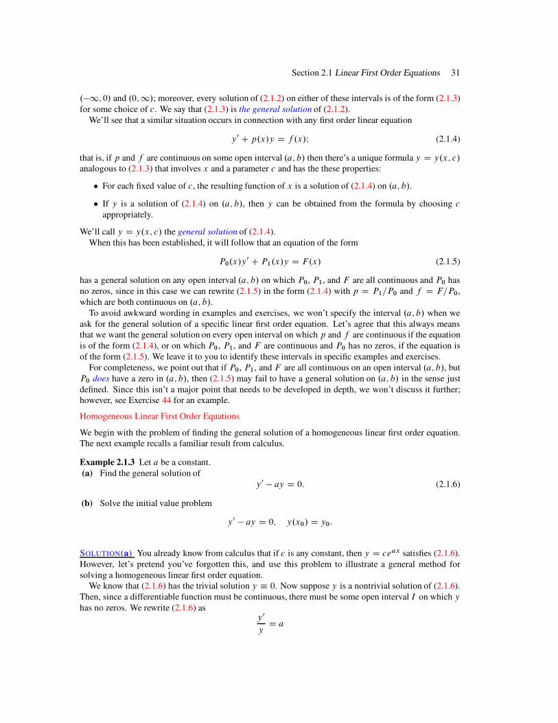
SOLUTION(a) You already know from calculus that if c is any constant, then y D ceax satisfies (2.1.6).However, let’s pretend you’ve forgotten this, and use this problem to illustrate a general method forsolving a homogeneous linear first order equation.
We know that (2.1.6) has the trivial solution y # 0. Now suppose y is a nontrivial solution of (2.1.6).Then, since a differentiable function must be continuous, there must be some open interval I on which yhas no zeros. We rewrite (2.1.6) as
y0
yD a
32 Chapter 2 First Order Equations
x0.2 0.4 0.6 0.8 1.0
y
0.5
1.0
1.5
2.0
2.5
3.0
a = 2
a = 1.5
a = 1
a = !1
a = !2.5
a = !4
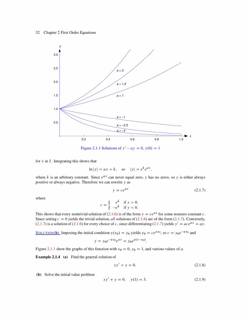
Figure 2.1.1 Solutions of y0 ! ay D 0, y.0/ D 1
for x in I . Integrating this shows that
ln jyj D ax C k; so jyj D ekeax;
where k is an arbitrary constant. Since eax can never equal zero, y has no zeros, so y is either alwayspositive or always negative. Therefore we can rewrite y as
y D ceax (2.1.7)
where
c D!
ek if y > 0;
!ek if y < 0:
This shows that every nontrivial solution of (2.1.6) is of the form y D ceax for some nonzero constant c.Since setting c D 0 yields the trivial solution, all solutions of (2.1.6) are of the form (2.1.7). Conversely,(2.1.7) is a solution of (2.1.6) for every choice of c, since differentiating (2.1.7) yields y0 D aceax D ay.
SOLUTION(b) Imposing the initial condition y.x0/ D y0 yields y0 D ceax0, so c D y0e!ax0 and
y D y0e!ax0eax D y0e
a.x!x0/:
Figure 2.1.1 show the graphs of this function with x0 D 0, y0 D 1, and various values of a.
Example 2.1.4 (a) Find the general solution of
xy0 C y D 0: (2.1.8)
(b) Solve the initial value problemxy0 C y D 0; y.1/ D 3: (2.1.9)
Section 2.1 Linear First Order Equations 33
SOLUTION(a) We rewrite (2.1.8) as
y0 C1
xy D 0; (2.1.10)
where x is restricted to either .!1; 0/ or .0;1/. If y is a nontrivial solution of (2.1.10), there must besome open interval I on which y has no zeros. We can rewrite (2.1.10) as
y0
yD !
1
x
for x in I . Integrating shows that
ln jyj D ! ln jxj C k; so jyj Dek
jxj:
Since a function that satisfies the last equation can’t change sign on either .!1; 0/ or .0;1/, we canrewrite this result more simply as
y Dc
x(2.1.11)
where
c D!
ek if y > 0;!ek if y < 0:
We’ve now shown that every solution of (2.1.10) is given by (2.1.11) for some choice of c. (Even thoughwe assumed that y was nontrivial to derive (2.1.11), we can get the trivial solution by setting c D 0 in(2.1.11).) Conversely, any function of the form (2.1.11) is a solution of (2.1.10), since differentiating(2.1.11) yields
y0 D !c
x2;
and substituting this and (2.1.11) into (2.1.10) yields
y0 C1
xy D !
c
x2C1
x
c
x
D !c
x2C
c
x2D 0:
Figure 2.1.2 shows the graphs of some solutions corresponding to various values of c
SOLUTION(b) Imposing the initial condition y.1/ D 3 in (2.1.11) yields c D 3. Therefore the solutionof (2.1.9) is
y D3
x:
The interval of validity of this solution is .0;1/.The results in Examples 2.1.3(a) and 2.1.4(b) are special cases of the next theorem.
Theorem 2.1.1 If p is continuous on .a; b/; then the general solution of the homogeneous equation
y0 C p.x/y D 0 (2.1.12)
on .a; b/ is
y D ce!P.x/;
where
P.x/ DZ
p.x/ dx (2.1.13)

34 Chapter 2 First Order Equations
x
y
c > 0 c < 0
c > 0 c < 0
Figure 2.1.2 Solutions of xy0 C y D 0 on .0;1/ and .!1; 0/
is any antiderivative of p on .a; b/I that is;
P 0.x/ D p.x/; a < x < b: (2.1.14)
Proof If y D ce!P.x/, differentiating y and using (2.1.14) shows that
y0 D !P 0.x/ce!P.x/ D !p.x/ce!P.x/ D !p.x/y;
so y0 C p.x/y D 0; that is, y is a solution of (2.1.12), for any choice of c.Now we’ll show that any solution of (2.1.12) can be written as y D ce!P.x/ for some constant c. The
trivial solution can be written this way, with c D 0. Now suppose y is a nontrivial solution. Then there’san open subinterval I of .a; b/ on which y has no zeros. We can rewrite (2.1.12) as
y0
yD !p.x/ (2.1.15)
for x in I . Integrating (2.1.15) and recalling (2.1.13) yields
ln jyj D !P.x/C k;
where k is a constant. This implies that
jyj D eke!P.x/:
Since P is defined for all x in .a; b/ and an exponential can never equal zero, we can take I D .a; b/, soy has zeros on .a; b/ .a; b/, so we can rewrite the last equation as y D ce!P.x/, where
c D!
ek if y > 0 on .a; b/;!ek if y < 0 on .a; b/:

Section 2.1 Linear First Order Equations 35
REMARK: Rewriting a first order differential equation so that one side depends only on y and y0 and theother depends only on x is called separation of variables. We did this in Examples 2.1.3 and 2.1.4, andin rewriting (2.1.12) as (2.1.15).We’llapply this method to nonlinear equations in Section 2.2.
Linear Nonhomogeneous First Order Equations
We’ll now solve the nonhomogeneous equation
y0 C p.x/y D f .x/: (2.1.16)
When considering this equation we call
y0 C p.x/y D 0
the complementary equation.We’ll find solutions of (2.1.16) in the form y D uy1, where y1 is a nontrivial solution of the com-
plementary equation and u is to be determined. This method of using a solution of the complementaryequation to obtain solutions of a nonhomogeneous equation is a special case of a method called variation
of parameters, which you’ll encounter several times in this book. (Obviously, u can’t be constant, sinceif it were, the left side of (2.1.16) would be zero. Recognizing this, the early users of this method viewedu as a “parameter” that varies; hence, the name “variation of parameters.”)
Ify D uy1; then y0 D u0y1 C uy0
1:
Substituting these expressions for y and y0 into (2.1.16) yields
u0y1 C u.y01 C p.x/y1/ D f .x/;
which reduces tou0y1 D f .x/; (2.1.17)
since y1 is a solution of the complementary equation; that is,
y01 C p.x/y1 D 0:
In the proof of Theorem 2.2.1 we saw that y1 has no zeros on an interval where p is continuous. Thereforewe can divide (2.1.17) through by y1 to obtain
u0 D f .x/=y1.x/:
We can integrate this (introducing a constant of integration), and multiply the result by y1 to get the gen-eral solution of (2.1.16). Before turning to the formal proof of this claim, let’s consider some examples.
Example 2.1.5 Find the general solution of
y0 C 2y D x3e!2x : (2.1.18)
By applying (a) of Example 2.1.3 with a D !2, we see that y1 D e!2x is a solution of the com-plementary equation y0 C 2y D 0. Therefore we seek solutions of (2.1.18) in the form y D ue!2x, sothat
y0 D u0e!2x ! 2ue!2x and y0 C 2y D u0e!2x ! 2ue!2x C 2ue!2x D u0e!2x: (2.1.19)
Therefore y is a solution of (2.1.18) if and only if
u0e!2x D x3e!2x or, equivalently, u0 D x3:
36 Chapter 2 First Order Equations
!1 !0.8 !0.6 !0.4 !0.2 0 0.2 0.4 0.6 0.8 1!2
!1.5
!1
!0.5
0
0.5
1
1.5
2
x
y
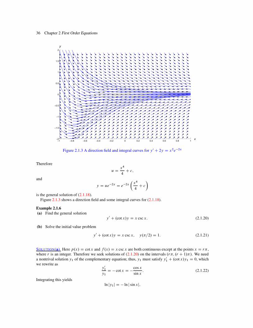
Figure 2.1.3 A direction field and integral curves for y0 C 2y D x2e!2x
Therefore
u Dx4
4C c;
and
y D ue!2x D e!2x
!
x4
4C c
"
is the general solution of (2.1.18).Figure 2.1.3 shows a direction field and some integral curves for (2.1.18).
Example 2.1.6(a) Find the general solution
y0 C .cot x/y D x csc x: (2.1.20)
(b) Solve the initial value problem
y0 C .cot x/y D x csc x; y.!=2/ D 1: (2.1.21)
SOLUTION(a) Here p.x/ D cotx and f .x/ D x csc x are both continuous except at the points x D r! ,where r is an integer. Therefore we seek solutions of (2.1.20) on the intervals .r!; .r C 1/!/. We needa nontrival solution y1 of the complementary equation; thus, y1 must satisfy y0
1 C .cot x/y1 D 0, whichwe rewrite as
y01
y1D ! cotx D !
cos x
sin x: (2.1.22)
Integrating this yieldsln jy1j D ! ln j sinxj;
Section 2.1 Linear First Order Equations 37
where we take the constant of integration to be zero since we need only one function that satisfies (2.1.22).Clearly y1 D 1= sinx is a suitable choice. Therefore we seek solutions of (2.1.20) in the form
y Du
sin x;
so that
y0 Du0
sinx!u cos x
sin2 x(2.1.23)
and
y0 C .cot x/y Du0
sin x!u cos x
sin2 xCu cot x
sinx
Du0
sin x!u cos x
sin2 xCu cos x
sin2 x
Du0
sin x:
(2.1.24)
Therefore y is a solution of (2.1.20) if and only if
u0= sinx D x csc x D x= sinx or, equivalently, u0 D x:
Integrating this yields
u Dx2
2C c; and y D
u
sinxD
x2
2 sinxC
c
sinx: (2.1.25)
is the general solution of (2.1.20) on every interval .r!; .r C 1/!/ (r Dinteger).
SOLUTION(b) Imposing the initial condition y.!=2/ D 1 in (2.1.25) yields
1 D!2
8C c or c D 1!
!2
8:
Thus,
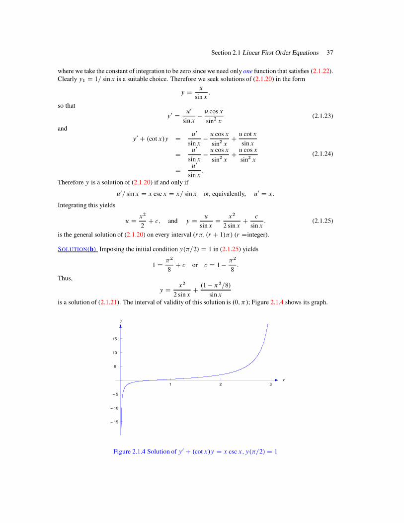
y Dx2
2 sinxC.1 ! !2=8/
sinxis a solution of (2.1.21). The interval of validity of this solution is .0;!/; Figure 2.1.4 shows its graph.
1 2 3
! 15
! 10
! 5
5
10
15
x
y
Figure 2.1.4 Solution of y0 C .cot x/y D x csc x; y.!=2/ D 1
38 Chapter 2 First Order Equations
REMARK: It wasn’t necessary to do the computations (2.1.23) and (2.1.24) in Example 2.1.6, since weshowed in the discussion preceding Example 2.1.5 that if y D uy1 where y0
1 C p.x/y1 D 0, theny0Cp.x/y D u0y1. We did these computations so you would see this happen in this specific example. Werecommend that you include these “unnecesary” computations in doing exercises, until you’re confidentthat you really understand the method. After that, omit them.
We summarize the method of variation of parameters for solving
y0 C p.x/y D f .x/ (2.1.26)
as follows:
(a) Find a function y1 such thaty0
1
y1D !p.x/:
For convenience, take the constant of integration to be zero.
(b) Writey D uy1 (2.1.27)
to remind yourself of what you’re doing.
(c) Write u0y1 D f and solve for u0; thus, u0 D f=y1.
(d) Integrate u0 to obtain u, with an arbitrary constant of integration.
(e) Substitute u into (2.1.27) to obtain y.
To solve an equation written as
P0.x/y0 C P1.x/y D F.x/;
we recommend that you divide through by P0.x/ to obtain an equation of the form (2.1.26) and thenfollow this procedure.
Solutions in Integral Form
Sometimes the integrals that arise in solving a linear first order equation can’t be evaluated in terms ofelementary functions. In this case the solution must be left in terms of an integral.
Example 2.1.7
(a) Find the general solution ofy0 ! 2xy D 1:
(b) Solve the initial value problem
y0 ! 2xy D 1; y.0/ D y0: (2.1.28)
SOLUTION(a) To apply variation of parameters, we need a nontrivial solution y1 of the complementaryequation; thus, y0
1 ! 2xy1 D 0, which we rewrite as
y01
y1D 2x:

Section 2.1 Linear First Order Equations 39
Integrating this and taking the constant of integration to be zero yields
ln jy1j D x2; so jy1j D ex2
:
We choose y1 D ex2and seek solutions of (2.1.28) in the form y D uex2
, where
u0ex2
D 1; so u0 D e!x2
:
Therefore
u D c CZ
e!x2
dx;
but we can’t simplify the integral on the right because there’s no elementary function with derivative
equal to e!x2. Therefore the best available form for the general solution of (2.1.28) is
y D uex2
D ex2
!
c CZ
e!x2
dx
"
: (2.1.29)
SOLUTION(b) Since the initial condition in (2.1.28) is imposed at x0 D 0, it is convenient to rewrite(2.1.29) as
y D ex2
!
c CZ x
0
e!t2dt
"
; since
Z 0
0
e!t2dt D 0:
Setting x D 0 and y D y0 here shows that c D y0. Therefore the solution of the initial value problem is
y D ex2
!
y0 CZ x
0e!t2
dt
"
: (2.1.30)
For a given value of y0 and each fixed x, the integral on the right can be evaluated by numerical methods.An alternate procedure is to apply the numerical integration procedures discussed in Chapter 3 directly tothe initial value problem (2.1.28). Figure 2.1.5 shows graphs of of (2.1.30) for several values of y0.
x
y
Figure 2.1.5 Solutions of y0 ! 2xy D 1, y.0/ D y0
40 Chapter 2 First Order Equations
An Existence and Uniqueness Theorem
The method of variation of parameters leads to this theorem.
Theorem 2.1.2 Suppose p and f are continuous on an open interval .a; b/; and let y1 be any nontrivial
solution of the complementary equation
y0 C p.x/y D 0
on .a; b/. ThenW(a) The general solution of the nonhomogeneous equation
y0 C p.x/y D f .x/ (2.1.31)
on .a; b/ is
y D y1.x/
!
c CZ
f .x/=y1.x/ dx
"
: (2.1.32)
(b) If x0 is an arbitrary point in .a; b/ and y0 is an arbitrary real number; then the initial value problem
y0 C p.x/y D f .x/; y.x0/ D y0
has the unique solution
y D y1.x/
!
y0
y1.x0/CZ x
x0
f .t/
y1.t/dt
"
on .a; b/:
Proof (a) To show that (2.1.32) is the general solution of (2.1.31) on .a; b/, we must prove that:(i) If c is any constant, the function y in (2.1.32) is a solution of (2.1.31) on .a; b/.
(ii) If y is a solution of (2.1.31) on .a; b/ then y is of the form (2.1.32) for some constant c.To prove (i), we first observe that any function of the form (2.1.32) is defined on .a; b/, since p and f
are continuous on .a; b/. Differentiating (2.1.32) yields
y0 D y01.x/
!
c CZ
f .x/=y1.x/ dx
"
C f .x/:
Since y01 D !p.x/y1, this and (2.1.32) imply that
y0 D !p.x/y1.x/
!
c CZ
f .x/=y1.x/ dx
"
C f .x/
D !p.x/y.x/ C f .x/;
which implies that y is a solution of (2.1.31).To prove (ii), suppose y is a solution of (2.1.31) on .a; b/. From the proof of Theorem 2.1.1, we know
that y1 has no zeros on .a; b/, so the function u D y=y1 is defined on .a; b/. Moreover, since
y0 D !py C f and y01 D !py1;
u0 Dy1y
0 ! y01y
y21
Dy1.!py C f /! .!py1/y
y21
Df
y1:

Section 2.1 Linear First Order Equations 41
Integrating u0 D f=y1 yields
u D!
c CZ
f .x/=y1.x/ dx
"
;
which implies (2.1.32), since y D uy1.(b) We’ve proved (a), where
R
f .x/=y1.x/ dx in (2.1.32) is an arbitrary antiderivative of f=y1. Nowit’s convenient to choose the antiderivative that equals zero when x D x0, and write the general solutionof (2.1.31) as
y D y1.x/
!
c CZ x
x0
f .t/
y1.t/dt
"
:
Since
y.x0/ D y1.x0/
!
c CZ x0
x0
f .t/
y1.t/dt
"
D cy1.x0/;
we see that y.x0/ D y0 if and only if c D y0=y1.x0/.
2.1 Exercises
In Exercises 1–5 find the general solution.
1. y0 C ay D 0 (a=constant) 2. y0 C 3x2y D 0
3. xy0 C .ln x/y D 0 4. xy0 C 3y D 0
5. x2y0 C y D 0
In Exercises 6–11 solve the initial value problem.
6. y0 C!
1C x
x
"
y D 0; y.1/ D 1
7. xy0 C!
1C1
lnx
"
y D 0; y.e/ D 1
8. xy0 C .1 C x cot x/y D 0; y#!
2
$
D 2
9. y0 !!
2x
1C x2
"
y D 0; y.0/ D 2
10. y0 Ck
xy D 0; y.1/ D 3 (k= constant)
11. y0 C .tan kx/y D 0; y.0/ D 2 (k D constant)
In Exercises 12 –15 find the general solution. Also, plot a direction field and some integral curves on the
rectangular region f!2 " x " 2; !2 " y " 2}.
12. C/G y0 C 3y D 1 13. C/G y0 C!
1
x! 1
"
y D !2
x
14. C/G y0 C 2xy D xe!x2
15. C/G y0 C2x
1C x2y D
e!x
1C x2
42 Chapter 2 First Order Equations
In Exercises 16 –24 find the general solution.
16. y0 C1
xy D
7
x2C 3 17. y0 C
4
x ! 1y D
1
.x ! 1/5C
sinx
.x ! 1/4
18. xy0 C .1 C 2x2/y D x3e!x2 19. xy0 C 2y D2
x2C 1
20. y0 C .tan x/y D cos x 21. .1C x/y0 C 2y Dsin x
1C x
22. .x ! 2/.x ! 1/y0 ! .4x ! 3/y D .x ! 2/3
23. y0 C .2 sin x cos x/y D e! sin2 x 24. x2y0 C 3xy D ex
In Exercises 25–29 solve the initial value problem and sketch the graph of the solution.
25. C/G y0 C 7y D e3x; y.0/ D 0
26. C/G .1 C x2/y0 C 4xy D2
1C x2; y.0/ D 1
27. C/G xy0 C 3y D2
x.1C x2/; y.!1/ D 0
28. C/G y0 C .cot x/y D cos x; y!!
2
"
D 1
29. C/G y0 C1
xy D
2
x2C 1; y.!1/ D 0
In Exercises 30–37 solve the initial value problem.
30. .x ! 1/y0 C 3y D1
.x ! 1/3C
sinx
.x ! 1/2; y.0/ D 1
31. xy0 C 2y D 8x2; y.1/ D 3
32. xy0 ! 2y D !x2; y.1/ D 1
33. y0 C 2xy D x; y.0/ D 3
34. .x ! 1/y0 C 3y D1C .x ! 1/ sec2 x
.x ! 1/3; y.0/ D !1
35. .x C 2/y0 C 4y D1C 2x2
x.x C 2/3; y.!1/ D 2
36. .x2 ! 1/y0 ! 2xy D x.x2 ! 1/; y.0/ D 4
37. .x2 ! 5/y0 ! 2xy D !2x.x2 ! 5/; y.2/ D 7
In Exercises 38–42 solve the initial value problem and leave the answer in a form involving a definite
integral. .You can solve these problems numerically by methods discussed in Chapter 3./
38. y0 C 2xy D x2; y.0/ D 3
39. y0 C1
xy D
sin x
x2; y.1/ D 2

Section 2.1 Linear First Order Equations 43
40. y0 C y De!x tan x
x; y.1/ D 0
41. y0 C2x
1C x2y D
ex
.1 C x2/2; y.0/ D 1
42. xy0 C .x C 1/y D ex2; y.1/ D 2
43. Experiments indicate that glucose is absorbed by the body at a rate proportional to the amount ofglucose present in the bloodstream. Let ! denote the (positive) constant of proportionality. Nowsuppose glucose is injected into a patient’s bloodstream at a constant rate of r units per unit oftime. Let G D G.t/ be the number of units in the patient’s bloodstream at time t > 0. Then
G0 D !!G C r;
where the first term on the right is due to the absorption of the glucose by the patient’s body andthe second term is due to the injection. Determine G for t > 0, given that G.0/ D G0. Also, findlimt!1 G.t/.
44. (a) L Plot a direction field and some integral curves for
xy0 ! 2y D !1 .A/
on the rectangular region f!1 " x " 1;!:5 " y " 1:5g. What do all the integral curveshave in common?
(b) Show that the general solution of (A) on .!1; 0/ and .0;1/ is
y D1
2C cx2:
(c) Show that y is a solution of (A) on .!1;1/ if and only if
y D
8
ˆ
<
ˆ
:
1
2C c1x
2; x # 0;
1
2C c2x
2; x < 0;
where c1 and c2 are arbitrary constants.
(d) Conclude from (c) that all solutions of (A) on .!1;1/ are solutions of the initial valueproblem
xy0 ! 2y D !1; y.0/ D1
2:
(e) Use (b) to show that if x0 ¤ 0 and y0 is arbitrary, then the initial value problem
xy0 ! 2y D !1; y.x0/ D y0
has infinitely many solutions on (!1;1). Explain why this does’nt contradict Theorem 2.1.1(b).
45. Suppose f is continuous on an open interval .a; b/ and ˛ is a constant.
(a) Derive a formula for the solution of the initial value problem
y0 C ˛y D f .x/; y.x0/ D y0; .A/
where x0 is in .a; b/ and y0 is an arbitrary real number.

44 Chapter 2 First Order Equations
(b) Suppose .a; b/ D .a;1/, ˛ > 0 and limx!1
f .x/ D L. Show that if y is the solution of (A),
then limx!1
y.x/ D L=˛.
46. Assume that all functions in this exercise are defined on a common interval .a; b/.
(a) Prove: If y1 and y2 are solutions of
y0 C p.x/y D f1.x/
andy0 C p.x/y D f2.x/
respectively, and c1 and c2 are constants, then y D c1y1 C c2y2 is a solution of
y0 C p.x/y D c1f1.x/C c2f2.x/:
(This is theprinciple of superposition.)
(b) Use (a) to show that if y1 and y2 are solutions of the nonhomogeneous equation
y0 C p.x/y D f .x/; .A/
then y1 ! y2 is a solution of the homogeneous equation
y0 C p.x/y D 0: .B/
(c) Use (a) to show that if y1 is a solution of (A) and y2 is a solution of (B), then y1 C y2 is asolution of (A).
47. Some nonlinear equations can be transformed into linear equations by changing the dependentvariable. Show that if
g0.y/y0 C p.x/g.y/ D f .x/
where y is a function of x and g is a function of y, then the new dependent variable ´ D g.y/satisfies the linear equation
´0 C p.x/´ D f .x/:
48. Solve by the method discussed in Exercise 47.
(a) .sec2 y/y0 ! 3 tany D !1 (b) ey2
!
2yy0 C2
x
"
D1
x2
(c)xy0
yC 2 lny D 4x2 (d)
y0
.1 C y/2!
1
x.1C y/D !
3
x2
49. We’ve shown that if p and f are continuous on .a; b/ then every solution of
y0 C p.x/y D f .x/ .A/
on .a; b/ can be written as y D uy1, where y1 is a nontrivial solution of the complementaryequation for (A) and u0 D f=y1. Now suppose f , f 0, . . . , f .m/ and p, p0, . . . , p.m!1/ arecontinuous on .a; b/, where m is a positive integer, and define
f0 D f;
fj D f 0j !1 C pfj !1; 1 " j " m:
Show that
u.j C1/ Dfj
y1; 0 " j " m:

Section 2.2 Separable Equations 45
2.2 SEPARABLE EQUATIONS
A first order differential equation is separable if it can be written as
h.y/y0 D g.x/; (2.2.1)
where the left side is a product of y0 and a function of y and the right side is a function of x. Rewritinga separable differential equation in this form is called separation of variables. In Section 2.1 we usedseparation of variables to solve homogeneous linear equations. In this section we’ll apply this method tononlinear equations.
To see how to solve (2.2.1), let’s first assume that y is a solution. Let G.x/ andH.y/ be antiderivativesof g.x/ and h.y/; that is,
H 0.y/ D h.y/ and G0.x/ D g.x/: (2.2.2)
Then, from the chain rule,
d
dxH.y.x// D H 0.y.x//y0 .x/ D h.y/y0.x/:
Therefore (2.2.1) is equivalent tod
dxH.y.x// D
d
dxG.x/:
Integrating both sides of this equation and combining the constants of integration yields
H.y.x// D G.x/C c: (2.2.3)
Although we derived this equation on the assumption that y is a solution of (2.2.1), we can now view itdifferently: Any differentiable function y that satisfies (2.2.3) for some constant c is a solution of (2.2.1).To see this, we differentiate both sides of (2.2.3), using the chain rule on the left, to obtain
H 0.y.x//y0 .x/ D G0.x/;
which is equivalent toh.y.x//y0.x/ D g.x/
because of (2.2.2).In conclusion, to solve (2.2.1) it suffices to find functions G D G.x/ and H D H.y/ that satisfy
(2.2.2). Then any differentiable function y D y.x/ that satisfies (2.2.3) is a solution of (2.2.1).
Example 2.2.1 Solve the equationy0 D x.1C y2/:
Solution Separating variables yieldsy0
1C y2D x:
Integrating yields
tan!1 y Dx2
2C c
Therefore
y D tan
!
x2
2C c
"
:

46 Chapter 2 First Order Equations
Example 2.2.2
(a) Solve the equation
y0 D !x
y: (2.2.4)
(b) Solve the initial value problem
y0 D !x
y; y.1/ D 1: (2.2.5)
(c) Solve the initial value problem
y0 D !x
y; y.1/ D !2: (2.2.6)
SOLUTION(a) Separating variables in (2.2.4) yields
yy0 D !x:
Integrating yieldsy2
2D !
x2
2C c; or, equivalently, x2 C y2 D 2c:
The last equation shows that c must be positive if y is to be a solution of (2.2.4) on an open interval.Therefore we let 2c D a2 (with a > 0) and rewrite the last equation as
x2 C y2 D a2: (2.2.7)
This equation has two differentiable solutions for y in terms of x:
y Dpa2 ! x2; !a < x < a; (2.2.8)
andy D !
pa2 ! x2; !a < x < a: (2.2.9)
The solution curves defined by (2.2.8) are semicircles above the x-axis and those defined by (2.2.9) aresemicircles below the x-axis (Figure 2.2.1).
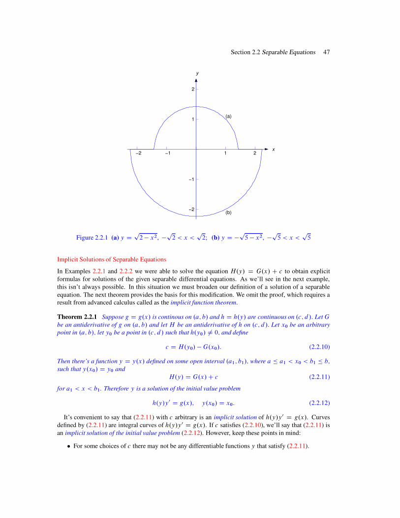
SOLUTION(b) The solution of (2.2.5) is positive when x D 1; hence, it is of the form (2.2.8). Substitutingx D 1 and y D 1 into (2.2.7) to satisfy the initial condition yields a2 D 2; hence, the solution of (2.2.5)is
y Dp2 ! x2; !
p2 < x <
p2:
SOLUTION(c) The solution of (2.2.6) is negative when x D 1 and is therefore of the form (2.2.9).Substituting x D 1 and y D !2 into (2.2.7) to satisfy the initial condition yields a2 D 5. Hence, thesolution of (2.2.6) is
y D !p5 ! x2; !
p5 < x <
p5:
Section 2.2 Separable Equations 47
x
y
1 2!1!2
1
2
!1
!2
(a)
(b)
Figure 2.2.1 (a) y Dp2 ! x2, !
p2 < x <
p2; (b) y D !
p5 ! x2, !
p5 < x <
p5
Implicit Solutions of Separable Equations
In Examples 2.2.1 and 2.2.2 we were able to solve the equation H.y/ D G.x/ C c to obtain explicitformulas for solutions of the given separable differential equations. As we’ll see in the next example,this isn’t always possible. In this situation we must broaden our definition of a solution of a separableequation. The next theorem provides the basis for this modification. We omit the proof, which requires aresult from advanced calculus called as the implicit function theorem.
Theorem 2.2.1 Suppose g D g.x/ is continous on .a; b/ and h D h.y/ are continuous on .c; d /: Let Gbe an antiderivative of g on .a; b/ and let H be an antiderivative of h on .c; d /: Let x0 be an arbitrarypoint in .a; b/; let y0 be a point in .c; d / such that h.y0/ ¤ 0; and define
c D H.y0/ !G.x0/: (2.2.10)
Then there’s a function y D y.x/ defined on some open interval .a1; b1/; where a " a1 < x0 < b1 " b;such that y.x0/ D y0 and
H.y/ D G.x/C c (2.2.11)
for a1 < x < b1. Therefore y is a solution of the initial value problem
h.y/y0 D g.x/; y.x0/ D x0: (2.2.12)
It’s convenient to say that (2.2.11) with c arbitrary is an implicit solution of h.y/y0 D g.x/. Curvesdefined by (2.2.11) are integral curves of h.y/y0 D g.x/. If c satisfies (2.2.10), we’ll say that (2.2.11) isan implicit solution of the initial value problem (2.2.12). However, keep these points in mind:
# For some choices of c there may not be any differentiable functions y that satisfy (2.2.11).
48 Chapter 2 First Order Equations
! The function y in (2.2.11) (not (2.2.11) itself) is a solution of h.y/y0 D g.x/.
Example 2.2.3
(a) Find implicit solutions of
y0 D2x C 1
5y4 C 1: (2.2.13)
(b) Find an implicit solution of
y0 D2x C 1
5y4 C 1; y.2/ D 1: (2.2.14)
SOLUTION(a) Separating variables yields
.5y4 C 1/y0 D 2x C 1:
Integrating yields the implicit solution
y5 C y D x2 C x C c: (2.2.15)
of (2.2.13).
SOLUTION(b) Imposing the initial condition y.2/ D 1 in (2.2.15) yields 1C 1 D 4C 2C c, so c D "4.Therefore
y5 C y D x2 C x " 4
is an implicit solution of the initial value problem (2.2.14). Although more than one differentiable func-tion y D y.x/ satisfies 2.2.13) near x D 1, it can be shown that there’s only one such function thatsatisfies the initial condition y.1/ D 2.
Figure 2.2.2 shows a direction field and some integral curves for (2.2.13).
Constant Solutions of Separable Equations
An equation of the formy0 D g.x/p.y/
is separable, since it can be rewritten as
1
p.y/y0 D g.x/:
However, the division by p.y/ is not legitimate if p.y/ D 0 for some values of y. The next two examplesshow how to deal with this problem.
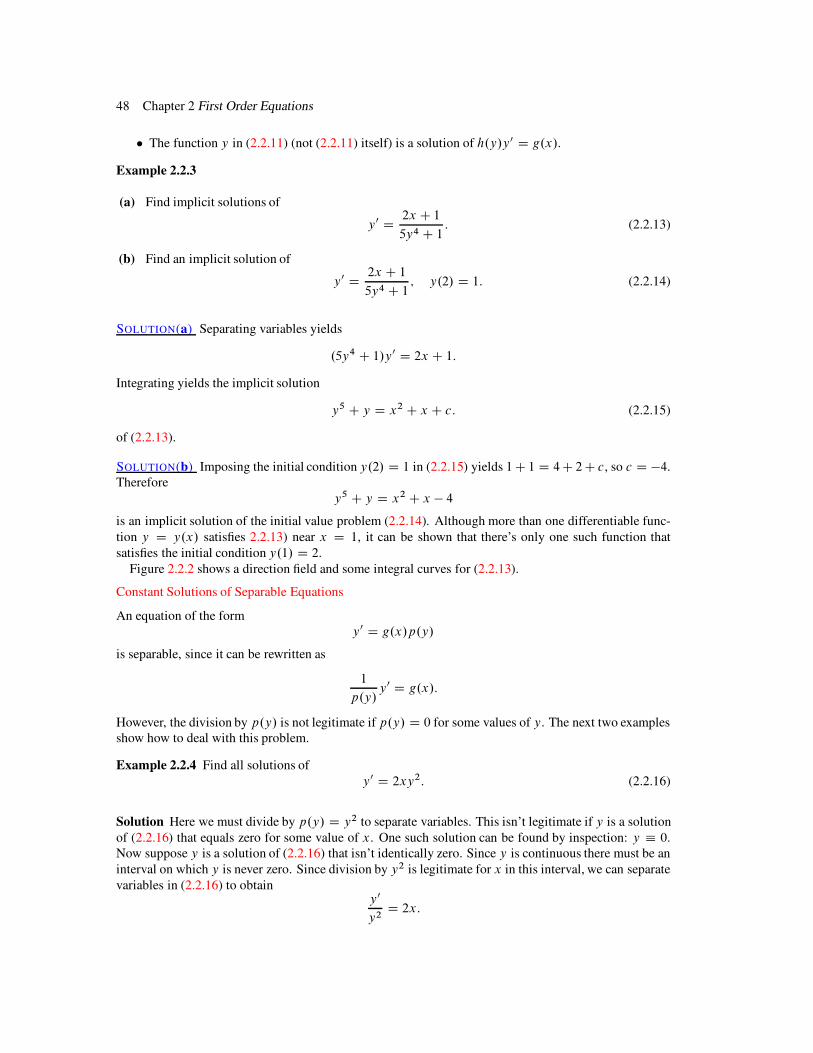
Example 2.2.4 Find all solutions ofy0 D 2xy2: (2.2.16)
Solution Here we must divide by p.y/ D y2 to separate variables. This isn’t legitimate if y is a solutionof (2.2.16) that equals zero for some value of x. One such solution can be found by inspection: y # 0.Now suppose y is a solution of (2.2.16) that isn’t identically zero. Since y is continuous there must be aninterval on which y is never zero. Since division by y2 is legitimate for x in this interval, we can separatevariables in (2.2.16) to obtain
y0
y2D 2x:

Section 2.2 Separable Equations 49
1 1.5 2 2.5 3 3.5 4!1
!0.5
0
0.5
1
1.5
2
x
y
Figure 2.2.2 A direction field and integral curves for y0 D2x C 1
5y4 C 1
Integrating this yields
!1
yD x2 C c;
which is equivalent to
y D !1
x2 C c: (2.2.17)
We’ve now shown that if y is a solution of (2.2.16) that is not identically zero, then y must be of theform (2.2.17). By substituting (2.2.17) into (2.2.16), you can verify that (2.2.17) is a solution of (2.2.16).Thus, solutions of (2.2.16) are y " 0 and the functions of the form (2.2.17). Note that the solution y " 0isn’t of the form (2.2.17) for any value of c.
Figure 2.2.3 shows a direction field and some integral curves for (2.2.16)
Example 2.2.5 Find all solutions of
y0 D1
2x.1 ! y2/: (2.2.18)
Solution Here we must divide by p.y/ D 1 ! y2 to separate variables. This isn’t legitimate if y is asolution of (2.2.18) that equals ˙1 for some value of x. Two such solutions can be found by inspection:y " 1 and y " !1. Now suppose y is a solution of (2.2.18) such that 1! y2 isn’t identically zero. Since1! y2 is continuous there must be an interval on which 1! y2 is never zero. Since division by 1! y2 islegitimate for x in this interval, we can separate variables in (2.2.18) to obtain
2y0
y2 ! 1D !x:
50 Chapter 2 First Order Equations
!2 !1.5 !1 !0.5 0 0.5 1 1.5 2!2
!1.5
!1
!0.5
0
0.5
1
1.5
2
y
x
Figure 2.2.3 A direction field and integral curves for y0 D 2xy2
A partial fraction expansion on the left yields
!
1
y ! 1!
1
y C 1
"
y0 D !x;
and integrating yields
ln
ˇ
ˇ
ˇ
ˇ
y ! 1y C 1
ˇ
ˇ
ˇ
ˇ
D !x2
2C kI
hence,ˇ
ˇ
ˇ
ˇ
y ! 1y C 1
ˇ
ˇ
ˇ
ˇ
D eke!x2=2:
Since y.x/ ¤ ˙1 for x on the interval under discussion, the quantity .y ! 1/=.y C 1/ can’t change signin this interval. Therefore we can rewrite the last equation as
y ! 1
y C 1D ce!x2=2;
where c D ˙ek, depending upon the sign of .y ! 1/=.y C 1/ on the interval. Solving for y yields
y D1C ce!x2=2
1 ! ce!x2=2: (2.2.19)
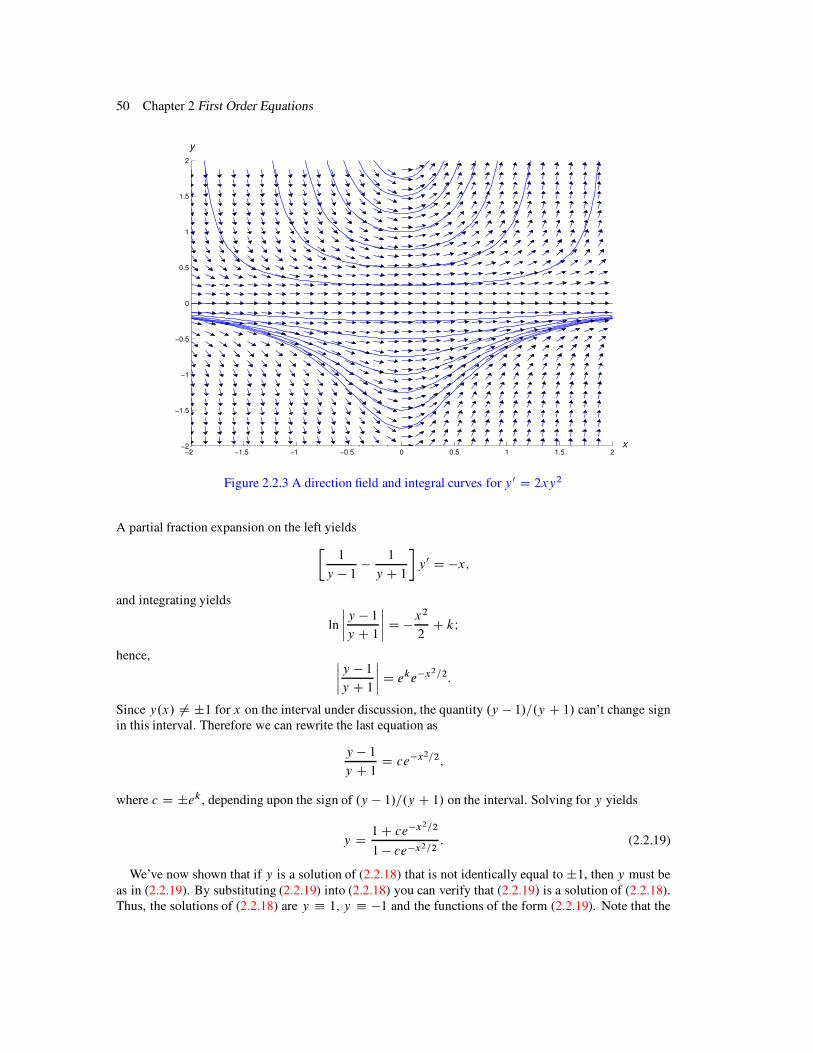
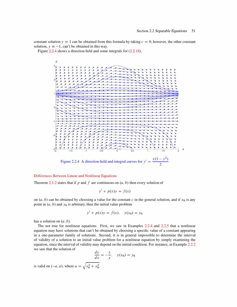
We’ve now shown that if y is a solution of (2.2.18) that is not identically equal to ˙1, then y must beas in (2.2.19). By substituting (2.2.19) into (2.2.18) you can verify that (2.2.19) is a solution of (2.2.18).Thus, the solutions of (2.2.18) are y " 1, y " !1 and the functions of the form (2.2.19). Note that the
Section 2.2 Separable Equations 51
constant solution y ! 1 can be obtained from this formula by taking c D 0; however, the other constantsolution, y ! "1, can’t be obtained in this way.
Figure 2.2.4 shows a direction field and some integrals for (2.2.18).
!2 !1.5 !1 !0.5 0 0.5 1 1.5 2!3
!2
!1
0
1
2
3
x
y
Figure 2.2.4 A direction field and integral curves for y0 Dx.1 " y2/
2
Differences Between Linear and Nonlinear Equations
Theorem 2.1.2 states that if p and f are continuous on .a; b/ then every solution of
y0 C p.x/y D f .x/
on .a; b/ can be obtained by choosing a value for the constant c in the general solution, and if x0 is anypoint in .a; b/ and y0 is arbitrary, then the initial value problem
y0 C p.x/y D f .x/; y.x0/ D y0
has a solution on .a; b/.The not true for nonlinear equations. First, we saw in Examples 2.2.4 and 2.2.5 that a nonlinear
equation may have solutions that can’t be obtained by choosing a specific value of a constant appearingin a one-parameter family of solutions. Second, it is in general impossible to determine the intervalof validity of a solution to an initial value problem for a nonlinear equation by simply examining theequation, since the interval of validity may depend on the initial condition. For instance, in Example 2.2.2we saw that the solution of
dy
dxD "
x
y; y.x0/ D y0
is valid on ."a; a/, where a Dq
x20 C y2
0 .
52 Chapter 2 First Order Equations
Example 2.2.6 Solve the initial value problem
y0 D 2xy2; y.0/ D y0
and determine the interval of validity of the solution.
Solution First suppose y0 ¤ 0. From Example 2.2.4, we know that y must be of the form
y D !1
x2 C c: (2.2.20)
Imposing the initial condition shows that c D !1=y0. Substituting this into (2.2.20) and rearrangingterms yields the solution
y Dy0
1 ! y0x2:
This is also the solution if y0 D 0. If y0 < 0, the denominator isn’t zero for any value of x, so the thesolution is valid on .!1;1/. If y0 > 0, the solution is valid only on .!1=py0; 1=
py0/.
2.2 Exercises
In Exercises 1–6 find all solutions.
1. y0 D3x2 C 2x C 1
y ! 22. .sin x/.sin y/C .cos y/y0 D 0
3. xy0 C y2 C y D 0 4. y0 ln jyj C x2y D 0
5. .3y3 C 3y cosy C 1/y0 C.2x C 1/y
1C x2D 0
6. x2yy0 D .y2 ! 1/3=2
In Exercises 7–10 find all solutions. Also, plot a direction field and some integral curves on the indicated
rectangular region.
7. C/G y0 D x2.1 C y2/I f!1 " x " 1; !1 " y " 1g
8. C/G y0.1C x2/C xy D 0I f!2 " x " 2; !1 " y " 1g
9. C/G y0 D .x ! 1/.y ! 1/.y ! 2/I f!2 " x " 2; !3 " y " 3g
10. C/G .y ! 1/2y0 D 2x C 3I f!2 " x " 2; !2 " y " 5g
In Exercises 11 and 12 solve the initial value problem.
11. y0 Dx2 C 3x C 2
y ! 2; y.1/ D 4
12. y0 C x.y2 C y/ D 0; y.2/ D 1
In Exercises 13-16 solve the initial value problem and graph the solution.
13. C/G .3y2 C 4y/y0 C 2x C cos x D 0; y.0/ D 1
Section 2.2 Separable Equations 53
14. C/G y0 C.y C 1/.y ! 1/.y ! 2/
x C 1D 0; y.1/ D 0
15. C/G y0 C 2x.y C 1/ D 0; y.0/ D 2
16. C/G y0 D 2xy.1 C y2/; y.0/ D 1
In Exercises 17–23 solve the initial value problem and find the interval of validity of the solution.
17. y0.x2 C 2/C 4x.y2 C 2y C 1/ D 0; y.1/ D !118. y0 D !2x.y2 ! 3y C 2/; y.0/ D 3
19. y0 D2x
1C 2y; y.2/ D 0 20. y0 D 2y ! y2; y.0/ D 1
21. x C yy0 D 0; y.3/ D !422. y0 C x2.y C 1/.y ! 2/2 D 0; y.4/ D 2
23. .x C 1/.x ! 2/y0 C y D 0; y.1/ D !3
24. Solve y0 D.1C y2/
.1 C x2/explicitly. HINT: Use the identity tan.AC B/ D
tanAC tanB
1 ! tanA tanB.
25. Solve y0p1 ! x2 C
p
1 ! y2 D 0 explicitly. HINT: Use the identity sin.A!B/ D sinA cosB !cosA sinB .
26. Solve y0 Dcos x
siny; y.!/ D
!
2explicitly. HINT: Use the identity cos.x C !=2/ D ! sinx and
the periodicity of the cosine.
27. Solve the initial value problem
y0 D ay ! by2; y.0/ D y0:
Discuss the behavior of the solution if (a) y0 " 0; (b) y0 < 0.
28. The populationP D P.t/ of a species satisfies the logistic equation
P 0 D aP.1 ! ˛P /
and P.0/ D P0 > 0. Find P for t > 0, and find limt!1 P.t/.
29. An epidemic spreads through a population at a rate proportional to the product of the number ofpeople already infected and the number of people susceptible, but not yet infected. Therefore, ifS denotes the total population of susceptible people and I D I.t/ denotes the number of infectedpeople at time t , then
I 0 D rI.S ! I /;
where r is a positive constant. Assuming that I.0/ D I0, find I.t/ for t > 0, and show thatlimt!1 I.t/ D S .
30. L The result of Exercise 29 is discouraging: if any susceptible member of the group is initiallyinfected, then in the long run all susceptible members are infected! On a more hopeful note,suppose the disease spreads according to the model of Exercise 29, but there’s a medication thatcures the infected population at a rate proportional to the number of infected individuals. Now theequation for the number of infected individuals becomes
I 0 D rI.S ! I / ! qI .A/
where q is a positive constant.

54 Chapter 2 First Order Equations
(a) Choose r and S positive. By plotting direction fields and solutions of (A) on suitable rectan-gular grids
R D f0 ! t ! T; 0 ! I ! d gin the .t; I /-plane, verify that if I is any solution of (A) such that I.0/ > 0, then limt!1 I.t/ DS " q=r if q < rS and limt!1 I.t/ D 0 if q # rS .
(b) To verify the experimental results of (a), use separation of variables to solve (A) with initialcondition I.0/ D I0 > 0, and find limt!1 I.t/. HINT: There are three cases to consider:
(i) q < rS ; (ii) q > rS ; (iii) q D rS .
31. L Consider the differential equation
y0 D ay " by2 " q; .A/
where a, b are positive constants, and q is an arbitrary constant. Suppose y denotes a solution ofthis equation that satisfies the initial condition y.0/ D y0.
(a) Choose a and b positive and q < a2=4b. By plotting direction fields and solutions of (A) onsuitable rectangular grids
R D f0 ! t ! T; c ! y ! d g .B/
in the .t; y/-plane, discover that there are numbers y1 and y2 with y1 < y2 such that ify0 > y1 then limt!1 y.t/ D y2, and if y0 < y1 then y.t/ D "1 for some finite value of t .(What happens if y0 D y1?)
(b) Choose a and b positive and q D a2=4b. By plotting direction fields and solutions of (A)on suitable rectangular grids of the form (B), discover that there’s a number y1 such that ify0 # y1 then limt!1 y.t/ D y1, while if y0 < y1 then y.t/ D "1 for some finite valueof t .
(c) Choose positive a, b and q > a2=4b. By plotting direction fields and solutions of (A) onsuitable rectangular grids of the form (B), discover that no matter what y0 is, y.t/ D "1for some finite value of t .
(d) Verify your results experiments analytically. Start by separating variables in (A) to obtain
y0
ay " by2 " qD 1:
To decide what to do next you’ll have to use the quadratic formula. This should lead you tosee why there are three cases. Take it from there!
Because of its role in the transition between these three cases, q0 D a2=4b is called abifurcation value of q. In general, if q is a parameter in any differential equation, q0 is saidto be a bifurcation value of q if the nature of the solutions of the equation with q < q0 isqualitatively different from the nature of the solutions with q > q0.
32. L By plotting direction fields and solutions of
y0 D qy " y3;
convince yourself that q0 D 0 is a bifurcation value of q for this equation. Explain what makesyou draw this conclusion.
33. Suppose a disease spreads according to the model of Exercise 29, but there’s a medication thatcures the infected population at a constant rate of q individuals per unit time, where q > 0. Thenthe equation for the number of infected individuals becomes
I 0 D rI.S " I / " q:
Assuming that I.0/ D I0 > 0, use the results of Exercise 31 to describe what happens as t ! 1.
Section 2.3 Existence and Uniqueness of Solutions of Nonlinear Equations 55
34. Assuming that p 6! 0, state conditions under which the linear equation
y0 C p.x/y D f .x/
is separable. If the equation satisfies these conditions, solve it by separation of variables and bythe method developed in Section 2.1.
Solve the equations in Exercises 35–38 using variation of parameters followed by separation of variables.
35. y0 C y D2xe!x
1C yex36. xy0 " 2y D
x6
y C x2
37. y0 " y D.x C 1/e4x
.y C ex/238. y0 " 2y D
xe2x
1 " ye!2x
39. Use variation of parameters to show that the solutions of the following equations are of the formy D uy1, where u satisfies a separable equation u0 D g.x/p.u/. Find y1 and g for each equation.
(a) xy0 C y D h.x/p.xy/ (b) xy0 " y D h.x/p!y
x
"
(c) y0 C y D h.x/p.exy/ (d) xy0 C ry D h.x/p.xry/
(e) y0 Cv0.x/
v.x/y D h.x/p .v.x/y/
2.3 EXISTENCE AND UNIQUENESS OF SOLUTIONS OF NONLINEAR EQUATIONS
Although there are methods for solving some nonlinear equations, it’s impossible to find useful formulasfor the solutions of most. Whether we’re looking for exact solutions or numerical approximations, it’suseful to know conditions that imply the existence and uniqueness of solutions of initial value problemsfor nonlinear equations. In this section we state such a condition and illustrate it with examples.
y
x a b
c
d
Figure 2.3.1 An open rectangle

56 Chapter 2 First Order Equations
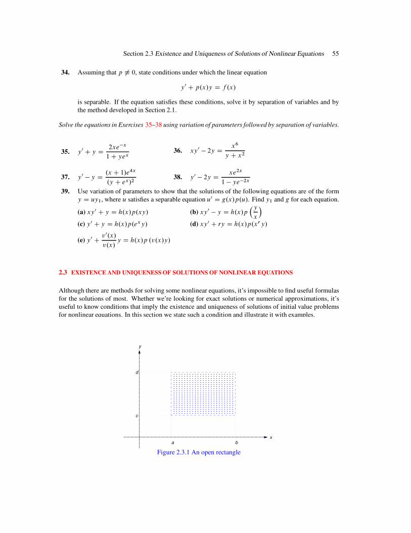
Some terminology: an open rectangle R is a set of points .x; y/ such that
a < x < b and c < y < d
(Figure 2.3.1). We’ll denote this set by R W fa < x < b; c < y < d g. “Open” means that the boundaryrectangle (indicated by the dashed lines in Figure 2.3.1) isn’t included in R .
The next theorem gives sufficient conditions for existence and uniqueness of solutions of initial valueproblems for first order nonlinear differential equations. We omit the proof, which is beyond the scope ofthis book.
Theorem 2.3.1
(a) If f is continuous on an open rectangle
R W fa < x < b; c < y < d g
that contains .x0; y0/ then the initial value problem
y0 D f .x; y/; y.x0/ D y0 (2.3.1)
has at least one solution on some open subinterval of .a; b/ that contains x0:
(b) If both f and fy are continuous on R then (2.3.1) has a unique solution on some open subinterval
of .a; b/ that contains x0.
It’s important to understand exactly what Theorem 2.3.1 says.
! (a) is an existence theorem. It guarantees that a solution exists on some open interval that containsx0, but provides no information on how to find the solution, or to determine the open interval onwhich it exists. Moreover, (a) provides no information on the number of solutions that (2.3.1) mayhave. It leaves open the possibility that (2.3.1) may have two or more solutions that differ for valuesof x arbitrarily close to x0. We will see in Example 2.3.6 that this can happen.
! (b) is a uniqueness theorem. It guarantees that (2.3.1) has a unique solution on some open interval(a,b) that contains x0. However, if .a; b/ ¤ ."1;1/, (2.3.1) may have more than one solutionon a larger interval that contains .a; b/. For example, it may happen that b < 1 and all solutionshave the same values on .a; b/, but two solutions y1 and y2 are defined on some interval .a; b1/with b1 > b, and have different values for b < x < b1; thus, the graphs of the y1 and y2 “branchoff” in different directions at x D b. (See Example 2.3.7 and Figure 2.3.3). In this case, continuityimplies that y1.b/ D y2.b/ (call their common value y), and y1 and y2 are both solutions of theinitial value problem
y0 D f .x; y/; y.b/ D y (2.3.2)
that differ on every open interval that contains b. Therefore f or fy must have a discontinuityat some point in each open rectangle that contains .b; y/, since if this were not so, (2.3.2) wouldhave a unique solution on some open interval that contains b. We leave it to you to give a similaranalysis of the case where a > "1.
Example 2.3.1 Consider the initial value problem
y0 Dx2 " y2
1C x2 C y2; y.x0/ D y0: (2.3.3)
Since
f .x; y/ Dx2 " y2
1C x2 C y2and fy.x; y/ D "
2y.1 C 2x2/
.1 C x2 C y2/2
Section 2.3 Existence and Uniqueness of Solutions of Nonlinear Equations 57
are continuous for all .x; y/, Theorem 2.3.1 implies that if .x0; y0/ is arbitrary, then (2.3.3) has a uniquesolution on some open interval that contains x0.
Example 2.3.2 Consider the initial value problem
y0 Dx2 ! y2
x2 C y2; y.x0/ D y0: (2.3.4)
Here
f .x; y/ Dx2 ! y2
x2 C y2and fy.x; y/ D !
4x2y
.x2 C y2/2
are continuous everywhere except at .0; 0/. If .x0; y0/ ¤ .0; 0/, there’s an open rectangle R that contains.x0; y0/ that does not contain .0; 0/. Since f and fy are continuous on R, Theorem 2.3.1 implies that if.x0; y0/ ¤ .0; 0/ then (2.3.4) has a unique solution on some open interval that contains x0.
Example 2.3.3 Consider the initial value problem
y0 Dx C y
x ! y; y.x0/ D y0: (2.3.5)
Here
f .x; y/ Dx C y
x ! yand fy.x; y/ D
2x
.x ! y/2
are continuous everywhere except on the line y D x. If y0 ¤ x0, there’s an open rectangleR that contains.x0; y0/ that does not intersect the line y D x. Since f and fy are continuous on R, Theorem 2.3.1implies that if y0 ¤ x0, (2.3.5) has a unique solution on some open interval that contains x0.
Example 2.3.4 In Example 2.2.4 we saw that the solutions of
y0 D 2xy2 (2.3.6)
are
y " 0 and y D !1
x2 C c;
where c is an arbitrary constant. In particular, this implies that no solution of (2.3.6) other than y " 0can equal zero for any value of x. Show that Theorem 2.3.1(b) implies this.
Solution We’ll obtain a contradiction by assuming that (2.3.6) has a solutiony1 that equals zero for somevalue of x, but isn’t identically zero. If y1 has this property, there’s a point x0 such that y1.x0/ D 0, buty1.x/ ¤ 0 for some value of x in every open interval that contains x0. This means that the initial valueproblem
y0 D 2xy2; y.x0/ D 0 (2.3.7)
has two solutions y " 0 and y D y1 that differ for some value of x on every open interval that containsx0. This contradicts Theorem 2.3.1(b), since in (2.3.6) the functions
f .x; y/ D 2xy2 and fy.x; y/ D 4xy:
are both continuous for all .x; y/, which implies that (2.3.7) has a unique solution on some open intervalthat contains x0.
58 Chapter 2 First Order Equations
Example 2.3.5 Consider the initial value problem
y0 D10
3xy2=5; y.x0/ D y0: (2.3.8)
(a) For what points .x0; y0/ does Theorem 2.3.1(a) imply that (2.3.8) has a solution?
(b) For what points .x0; y0/ does Theorem 2.3.1(b) imply that (2.3.8) has a unique solution on someopen interval that contains x0?
SOLUTION(a) Since
f .x; y/ D10
3xy2=5
is continuous for all .x; y/, Theorem 2.3.1 implies that (2.3.8) has a solution for every .x0; y0/.
SOLUTION(b) Here
fy.x; y/ D4
3xy!3=5
is continuous for all .x; y/ with y ¤ 0. Therefore, if y0 ¤ 0 there’s an open rectangle on which bothf and fy are continuous, and Theorem 2.3.1 implies that (2.3.8) has a unique solution on some openinterval that contains x0.
If y D 0 then fy.x; y/ is undefined, and therefore discontinuous; hence, Theorem 2.3.1 does not applyto (2.3.8) if y0 D 0.
Example 2.3.6 Example 2.3.5 leaves open the possibility that the initial value problem
y0 D10
3xy2=5; y.0/ D 0 (2.3.9)
has more than one solution on every open interval that contains x0 D 0. Show that this is true.
Solution By inspection, y ! 0 is a solution of the differential equation
y0 D10
3xy2=5: (2.3.10)
Since y ! 0 satisfies the initial condition y.0/ D 0, it’s a solution of (2.3.9).Now suppose y is a solution of (2.3.10) that isn’t identically zero. Separating variables in (2.3.10)
yields
y!2=5y0 D10
3x
on any open interval where y has no zeros. Integrating this and rewriting the arbitrary constant as 5c=3yields
5
3y3=5 D
5
3.x2 C c/:
Thereforey D .x2 C c/5=3: (2.3.11)
Since we divided by y to separate variables in (2.3.10), our derivation of (2.3.11) is legitimate only onopen intervals where y has no zeros. However, (2.3.11) actually defines y for all x, and differentiating(2.3.11) shows that
y0 D10
3x.x2 C c/2=3 D
10
3xy2=5; "1 < x < 1:
Section 2.3 Existence and Uniqueness of Solutions of Nonlinear Equations 59
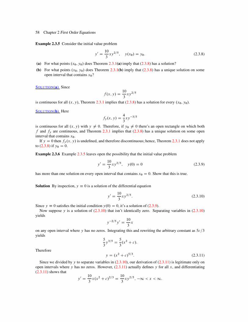
x
y
Figure 2.3.2 Two solutions (y D 0 and y D x1=2) of (2.3.9) that differ on every interval containingx0 D 0
Therefore (2.3.11) satisfies (2.3.10) on .!1;1/ even if c " 0, so that y.p
jcj/ D y.!p
jcj/ D 0. Inparticular, taking c D 0 in (2.3.11) yields
y D x10=3
as a second solution of (2.3.9). Both solutions are defined on .!1;1/, and they differ on every openinterval that contains x0 D 0 (see Figure 2.3.2.) In fact, there are four distinct solutions of (2.3.9) definedon .!1;1/ that differ from each other on every open interval that contains x0 D 0. Can you identifythe other two?
Example 2.3.7 From Example 2.3.5, the initial value problem
y0 D10
3xy2=5; y.0/ D !1 (2.3.12)
has a unique solution on some open interval that contains x0 D 0. Find a solution and determine thelargest open interval .a; b/ on which it’s unique.
Solution Let y be any solution of (2.3.12). Because of the initial condition y.0/ D !1 and the continuityof y, there’s an open interval I that contains x0 D 0 on which y has no zeros, and is consequently of theform (2.3.11). Setting x D 0 and y D !1 in (2.3.11) yields c D !1, so
y D .x2 ! 1/5=3 (2.3.13)
for x in I . Therefore every solution of (2.3.12) differs from zero and is given by (2.3.13) on .!1; 1/;that is, (2.3.13) is the unique solution of (2.3.12) on .!1; 1/. This is the largest open interval on which
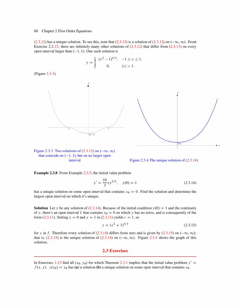
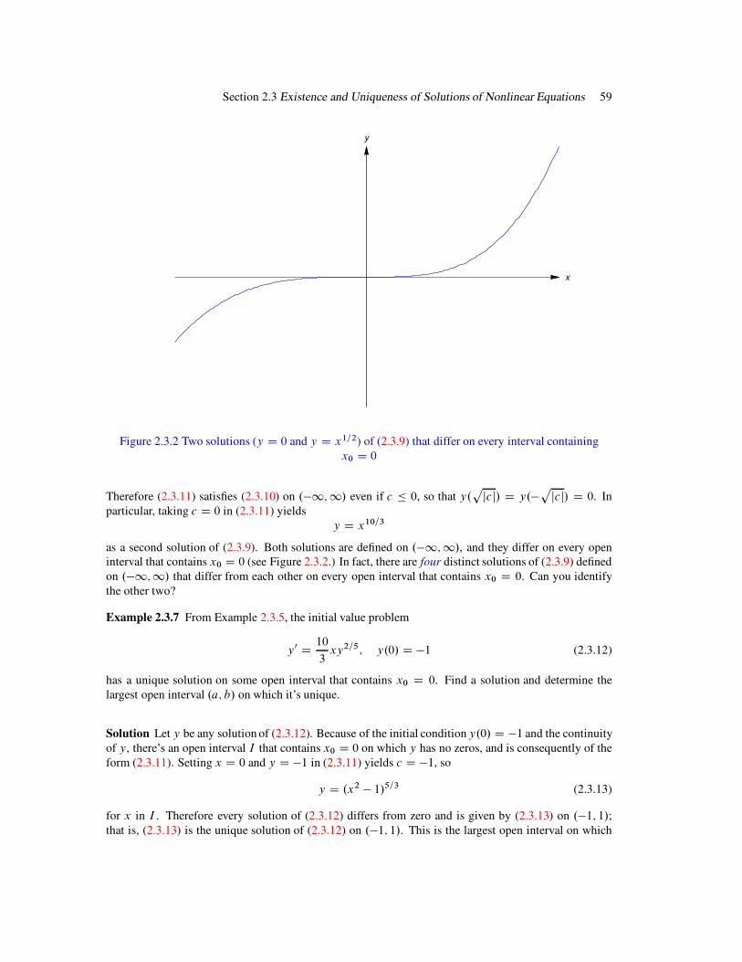
60 Chapter 2 First Order Equations
(2.3.12) has a unique solution. To see this, note that (2.3.13) is a solution of (2.3.12) on .!1;1/. FromExercise 2.2.15, there are infinitely many other solutions of (2.3.12) that differ from (2.3.13) on everyopen interval larger than .!1; 1/. One such solution is
y D
(
.x2 ! 1/5=3; !1 " x " 1;
0; jxj > 1:
(Figure 2.3.3).
1!1 x
y
(0, !1)
Figure 2.3.3 Two solutions of (2.3.12) on .!1;1/that coincide on .!1; 1/, but on no larger open
interval
x
y
(0,1)
Figure 2.3.4 The unique solution of (2.3.14)
Example 2.3.8 From Example 2.3.5, the initial value problem
y0 D10
3xy2=5; y.0/ D 1 (2.3.14)
has a unique solution on some open interval that contains x0 D 0. Find the solution and determine thelargest open interval on which it’s unique.
Solution Let y be any solution of (2.3.14). Because of the initial condition y.0/ D 1 and the continuityof y, there’s an open interval I that contains x0 D 0 on which y has no zeros, and is consequently of theform (2.3.11). Setting x D 0 and y D 1 in (2.3.11) yields c D 1, so
y D .x2 C 1/5=3 (2.3.15)
for x in I . Therefore every solution of (2.3.14) differs from zero and is given by (2.3.15) on .!1;1/;that is, (2.3.15) is the unique solution of (2.3.14) on .!1;1/. Figure 2.3.4 shows the graph of thissolution.
2.3 Exercises
In Exercises 1-13 find all .x0; y0/ for which Theorem 2.3.1 implies that the initial value problem y0 Df .x; y/; y.x0/ D y0 has (a) a solution (b) a unique solution on some open interval that contains x0.
Section 2.3 Existence and Uniqueness of Solutions of Nonlinear Equations 61
1. y0 Dx2 C y2
sin x2. y0 D
ex C y
x2 C y2
3. y0 D tanxy4. y0 D
x2 C y2
lnxy
5. y0 D .x2 C y2/y1=36. y0 D 2xy
7. y0 D ln.1C x2 C y2/ 8. y0 D2x C 3y
x ! 4y
9. y0 D .x2 C y2/1=2 10. y0 D x.y2 ! 1/2=3
11. y0 D .x2 C y2/2 12. y0 D .x C y/1=2
13. y0 Dtan y
x ! 114. Apply Theorem 2.3.1 to the initial value problem
y0 C p.x/y D q.x/; y.x0/ D y0
for a linear equation, and compare the conclusions that can be drawn from it to those that followfrom Theorem 2.1.2.
15. (a) Verify that the function
y D
(
.x2 ! 1/5=3; !1 < x < 1;
0; jxj " 1;
is a solution of the initial value problem
y0 D10
3xy2=5; y.0/ D !1
on .!1;1/. HINT: You’ll need the definition
y0.x/ D limx!x
y.x/ ! y.x/x ! x
to verify that y satisfies the differential equation at x D ˙1.
(b) Verify that if !i D 0 or 1 for i D 1, 2 and a, b > 1, then the function
y D
8
ˆ
ˆ
ˆ
ˆ
ˆ
ˆ
ˆ
ˆ
<
ˆ
ˆ
ˆ
ˆ
ˆ
ˆ
ˆ
ˆ
:
!1.x2 ! a2/5=3; !1 < x < !a;
0; !a # x # !1;
.x2 ! 1/5=3; !1 < x < 1;
0; 1 # x # b;
!2.x2 ! b2/5=3; b < x < 1;
is a solution of the initial value problem of (a) on .!1;1/.
62 Chapter 2 First Order Equations
16. Use the ideas developed in Exercise 15 to find infinitely many solutions of the initial value problem
y0 D y2=5; y.0/ D 1
on .!1;1/.
17. Consider the initial value problem
y0 D 3x.y ! 1/1=3; y.x0/ D y0: .A/
(a) For what points .x0; y0/ does Theorem 2.3.1 imply that (A) has a solution?
(b) For what points .x0; y0/ does Theorem 2.3.1 imply that (A) has a unique solution on someopen interval that contains x0?
18. Find nine solutions of the initial value problem
y0 D 3x.y ! 1/1=3; y.0/ D 1
that are all defined on .!1;1/ and differ from each other for values of x in every open intervalthat contains x0 D 0.
19. From Theorem 2.3.1, the initial value problem
y0 D 3x.y ! 1/1=3; y.0/ D 9
has a unique solution on an open interval that contains x0 D 0. Find the solution and determinethe largest open interval on which it’s unique.
20. (a) From Theorem 2.3.1, the initial value problem
y0 D 3x.y ! 1/1=3; y.3/ D !7 .A/
has a unique solution on some open interval that contains x0 D 3. Determine the largest suchopen interval, and find the solution on this interval.
(b) Find infinitely many solutions of (A), all defined on .!1;1/.
21. Prove:
(a) Iff .x; y0/ D 0; a < x < b; .A/
and x0 is in .a; b/, then y " y0 is a solution of
y0 D f .x; y/; y.x0/ D y0
on .a; b/.
(b) If f and fy are continuous on an open rectangle that contains .x0; y0/ and (A) holds, nosolution of y0 D f .x; y/ other than y " y0 can equal y0 at any point in .a; b/.
2.4 TRANSFORMATION OF NONLINEAR EQUATIONS INTO SEPARABLE EQUATIONS
In Section 2.1 we found that the solutions of a linear nonhomogeneous equation
y0 C p.x/y D f .x/

Section 2.4 Transformation of Nonlinear Equations into Separable Equations 63
are of the form y D uy1, where y1 is a nontrivial solution of the complementary equation
y0 C p.x/y D 0 (2.4.1)
and u is a solution ofu0y1.x/ D f .x/:
Note that this last equation is separable, since it can be rewritten as
u0 Df .x/
y1.x/:
In this section we’ll consider nonlinear differential equations that are not separable to begin with, but canbe solved in a similar fashion by writing their solutions in the form y D uy1, where y1 is a suitablychosen known function and u satisfies a separable equation. We’llsay in this case that we transformed
the given equation into a separable equation.
Bernoulli Equations
A Bernoulli equation is an equation of the form
y0 C p.x/y D f .x/yr ; (2.4.2)
where r can be any real number other than 0 or 1. (Note that (2.4.2) is linear if and only if r D 0or r D 1.) We can transform (2.4.2) into a separable equation by variation of parameters: if y1 is anontrivial solution of (2.4.1), substituting y D uy1 into (2.4.2) yields
u0y1 C u.y01 C p.x/y1/ D f .x/.uy1/
r ;
which is equivalent to the separable equation
u0y1.x/ D f .x/ .y1.x//r ur or
u0
urD f .x/ .y1.x//
r!1 ;
since y01 C p.x/y1 D 0.
Example 2.4.1 Solve the Bernoulli equation
y0 ! y D xy2: (2.4.3)
Solution Since y1 D ex is a solution of y0 !y D 0, we look for solutions of (2.4.3) in the form y D uex,where
u0ex D xu2e2x or, equivalently, u0 D xu2ex:
Separating variables yieldsu0
u2D xex;
and integrating yields
!1
uD .x ! 1/ex C c:
Hence,
u D !1
.x ! 1/ex C c
64 Chapter 2 First Order Equations
!2 !1.5 !1 !0.5 0 0.5 1 1.5 2!2
!1.5
!1
!0.5
0
0.5
1
1.5
2
x
y
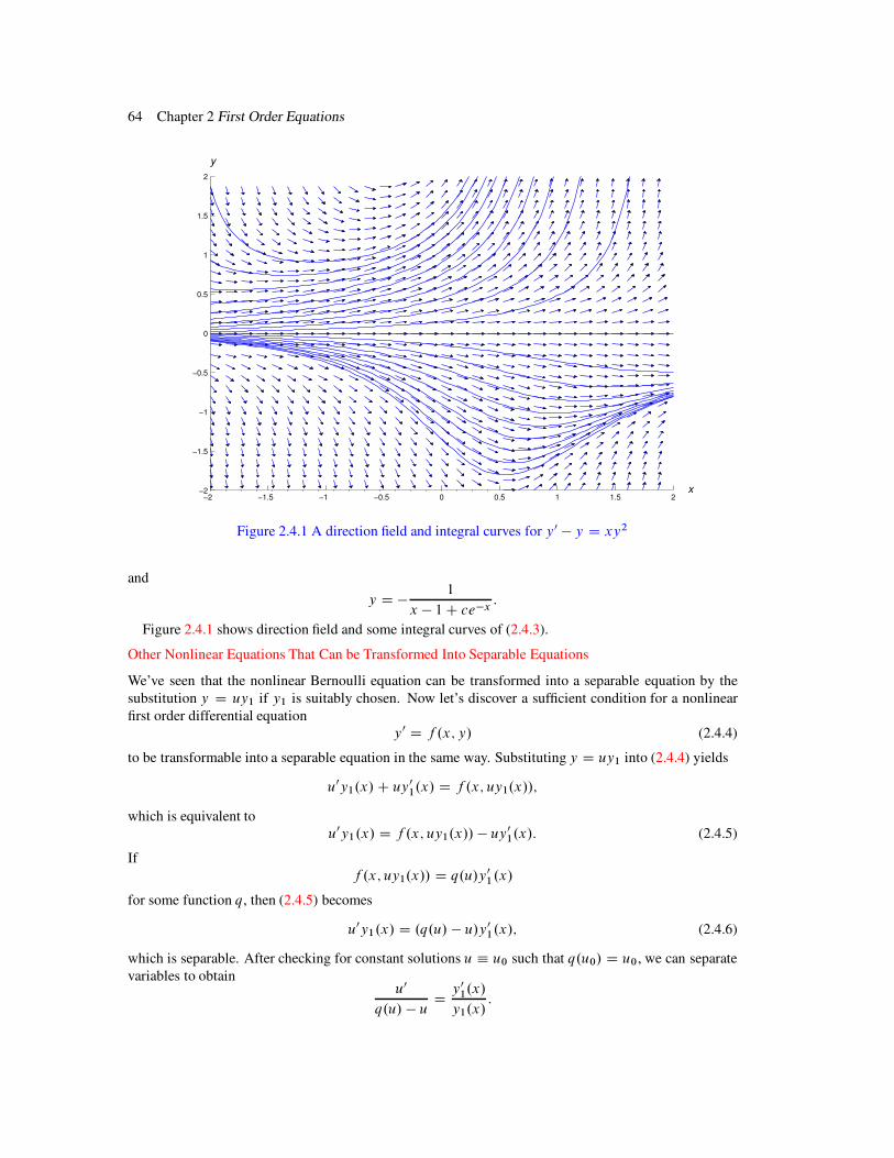
Figure 2.4.1 A direction field and integral curves for y0 ! y D xy2
and
y D !1
x ! 1C ce!x:
Figure 2.4.1 shows direction field and some integral curves of (2.4.3).
Other Nonlinear Equations That Can be Transformed Into Separable Equations
We’ve seen that the nonlinear Bernoulli equation can be transformed into a separable equation by thesubstitution y D uy1 if y1 is suitably chosen. Now let’s discover a sufficient condition for a nonlinearfirst order differential equation
y0 D f .x; y/ (2.4.4)
to be transformable into a separable equation in the same way. Substituting y D uy1 into (2.4.4) yields
u0y1.x/C uy01.x/ D f .x; uy1.x//;
which is equivalent tou0y1.x/ D f .x; uy1.x// ! uy0
1.x/: (2.4.5)
Iff .x; uy1.x// D q.u/y0
1.x/
for some function q, then (2.4.5) becomes
u0y1.x/ D .q.u/ ! u/y01.x/; (2.4.6)
which is separable. After checking for constant solutions u " u0 such that q.u0/ D u0, we can separatevariables to obtain
u0
q.u/ ! uDy0
1.x/
y1.x/:

Section 2.4 Transformation of Nonlinear Equations into Separable Equations 65
Homogeneous Nonlinear Equations
In the text we’ll consider only the most widely studied class of equations for which the method of thepreceding paragraph works. Other types of equations appear in Exercises 44–51.
The differential equation (2.4.4) is said to be homogeneous if x and y occur in f in such a way thatf .x; y/ depends only on the ratio y=x; that is, (2.4.4) can be written as
y0 D q.y=x/; (2.4.7)
where q D q.u/ is a function of a single variable. For example,
y0 Dy C xe!y=x
xDy
xC e!y=x
and
y0 Dy2 C xy ! x2
x2D!y
x
"2Cy
x! 1
are of the form (2.4.7), with
q.u/ D uC e!u and q.u/ D u2 C u! 1;
respectively. The general method discussed above can be applied to (2.4.7) with y1 D x (and thereforey0
1 D 1/. Thus, substituting y D ux in (2.4.7) yields
u0x C u D q.u/;
and separation of variables (after checking for constant solutions u " u0 such that q.u0/ D u0) yields
u0
q.u/ ! uD1
x:
Before turning to examples, we point out something that you may’ve have already noticed: the defini-tion of homogeneous equation given here isn’t the same as the definition given in Section 2.1, where wesaid that a linear equation of the form
y0 C p.x/y D 0
is homogeneous. We make no apology for this inconsistency, since we didn’t create it historically, homo-
geneous has been used in these two inconsistent ways. The one having to do with linear equations is themost important. This is the only section of the book where the meaning defined here will apply.
Since y=x is in general undefined if x D 0, we’ll consider solutions of nonhomogeneous equationsonly on open intervals that do not contain the point x D 0.
Example 2.4.2 Solve
y0 Dy C xe!y=x
x: (2.4.8)
Solution Substituting y D ux into (2.4.8) yields
u0x C u Dux C xe!ux=x
xD uC e!u:
Simplifying and separating variables yields
euu0 D1
x:
66 Chapter 2 First Order Equations
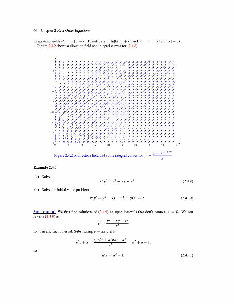
Integrating yields eu D ln jxj C c. Therefore u D ln.ln jxj C c/ and y D ux D x ln.ln jxj C c/.Figure 2.4.2 shows a direction field and integral curves for (2.4.8).
0.5 1 1.5 2 2.5 3 3.5 4 4.5 5!2
!1.5
!1
!0.5
0
0.5
1
1.5
2
x
y
Figure 2.4.2 A direction field and some integral curves for y0 Dy C xe!y=x
x
Example 2.4.3
(a) Solvex2y0 D y2 C xy ! x2: (2.4.9)
(b) Solve the initial value problem
x2y0 D y2 C xy ! x2; y.1/ D 2: (2.4.10)
SOLUTION(a) We first find solutions of (2.4.9) on open intervals that don’t contain x D 0. We canrewrite (2.4.9) as
y0 Dy2 C xy ! x2
x2
for x in any such interval. Substituting y D ux yields
u0x C u D.ux/2 C x.ux/ ! x2
x2D u2 C u! 1;
sou0x D u2 ! 1: (2.4.11)
Section 2.4 Transformation of Nonlinear Equations into Separable Equations 67
By inspection this equation has the constant solutions u ! 1 and u ! "1. Therefore y D x and y D "xare solutions of (2.4.9). If u is a solution of (2.4.11) that doesn’t assume the values ˙1 on some interval,separating variables yields
u0
u2 " 1D1
x;
or, after a partial fraction expansion,
1
2
!
1
u " 1"
1
uC 1
"
u0 D1
x:
Multiplying by 2 and integrating yields
ln
ˇ
ˇ
ˇ
ˇ
u" 1uC 1
ˇ
ˇ
ˇ
ˇ
D 2 ln jxj C k;
orˇ
ˇ
ˇ
ˇ
u " 1uC 1
ˇ
ˇ
ˇ
ˇ
D ekx2;
which holds ifu " 1uC 1
D cx2 (2.4.12)
where c is an arbitrary constant. Solving for u yields
u D1C cx2
1 " cx2:
!2 !1.5 !1 !0.5 0 0.5 1 1.5 2!2
!1.5
!1
!0.5
0
0.5
1
1.5
2
y
x
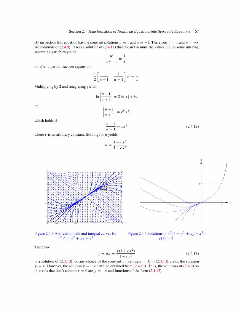
Figure 2.4.3 A direction field and integral curves forx2y0 D y2 C xy " x2
x
y
1
2
Figure 2.4.4 Solutions of x2y0 D y2 C xy " x2,y.1/ D 2
Therefore
y D ux Dx.1C cx2/
1 " cx2(2.4.13)
is a solution of (2.4.10) for any choice of the constant c. Setting c D 0 in (2.4.13) yields the solutiony D x. However, the solution y D "x can’t be obtained from (2.4.13). Thus, the solutions of (2.4.9) onintervals that don’t contain x D 0 are y D "x and functions of the form (2.4.13).
68 Chapter 2 First Order Equations
The situation is more complicated if x D 0 is the open interval. First, note that y D !x satisfies (2.4.9)on .!1;1/. If c1 and c2 are arbitrary constants, the function
y D
8
ˆ
ˆ
<
ˆ
ˆ
:
x.1C c1x2/
1 ! c1x2; a < x < 0;
x.1C c2x2/
1 ! c2x2; 0 " x < b;
(2.4.14)
is a solution of (2.4.9) on .a; b/, where
a D
8
<
:
!1
pc1
if c1 > 0;
!1 if c1 " 0;and b D
8
<
:
1pc2
if c2 > 0;
1 if c2 " 0:
We leave it to you to verify this. To do so, note that if y is any function of the form (2.4.13) then y.0/ D 0and y0.0/ D 1.
Figure 2.4.3 shows a direction field and some integral curves for (2.4.9).
SOLUTION(b) We could obtain c by imposing the initial condition y.1/ D 2 in (2.4.13), and then solvingfor c. However, it’s easier to use (2.4.12). Since u D y=x, the initial condition y.1/ D 2 implies thatu.1/ D 2. Substituting this into (2.4.12) yields c D 1=3. Hence, the solution of (2.4.10) is
y Dx.1C x2=3/
1 ! x2=3:
The interval of validity of this solution is .!p3;
p3/. However, the largest interval on which (2.4.10)
has a unique solution is .0;p3/. To see this, note from (2.4.14) that any function of the form
y D
8
ˆ
ˆ
<
ˆ
ˆ
:
x.1C cx2/
1 ! cx2; a < x " 0;
x.1C x2=3/
1 ! x2=3; 0 " x <
p3;
(2.4.15)
is a solution of (2.4.10) on .a;p3/, where a D !1=
pc if c > 0 or a D !1 if c " 0. (Why doesn’t this
contradict Theorem 2.3.1?)Figure 2.4.4 shows several solutions of the initial value problem (2.4.10). Note that these solutions
coincide on .0;p3/.
In the last two examples we were able to solve the given equations explicitly. However, this isn’t alwayspossible, as you’ll see in the exercises.
2.4 Exercises
In Exercises 1–4 solve the given Bernoulli equation.
1. y0 C y D y2 2. 7xy0 ! 2y D !x2
y6
3. x2y0 C 2y D 2e1=xy1=2 4. .1C x2/y0 C 2xy D1
.1 C x2/y
In Exercises 5 and 6 find all solutions. Also, plot a direction field and some integral curves on theindicated rectangular region.
Section 2.4 Transformation of Nonlinear Equations into Separable Equations 69
5. C/G y0 ! xy D x3y3I f!3 " x " 3; 2 " y # 2g
6. C/G y0 !1C x
3xy D y4I f!2 " x " 2;!2 " y " 2g
In Exercises 7–11 solve the initial value problem.
7. y0 ! 2y D xy3; y.0/ D 2p2
8. y0 ! xy D xy3=2; y.1/ D 4
9. xy0 C y D x4y4; y.1/ D 1=2
10. y0 ! 2y D 2y1=2; y.0/ D 1
11. y0 ! 4y D48x
y2; y.0/ D 1
In Exercises 12 and 13 solve the initial value problem and graph the solution.
12. C/G x2y0 C 2xy D y3; y.1/ D 1=p2
13. C/G y0 ! y D xy1=2; y.0/ D 4
14. You may have noticed that the logistic equation
P 0 D aP.1 ! ˛P /
from Verhulst’s model for population growth can be written in Bernoulli form as
P 0 ! aP D !a˛P 2:
This isn’t particularly interesting, since the logistic equation is separable, and therefore solvableby the method studied in Section 2.2. So let’s consider a more complicated model, where a isa positive constant and ˛ is a positive continuous function of t on Œ0;1/. The equation for thismodel is
P 0 ! aP D !a˛.t/P 2;
a non-separable Bernoulli equation.
(a) Assuming that P.0/ D P0 > 0, find P for t > 0. HINT: Express your result in terms of the
integralR t
0 ˛.!/ea! d! .
(b) Verify that your result reduces to the known results for the Malthusian model where ˛ D 0,and the Verhulst model where ˛ is a nonzero constant.
(c) Assuming that
limt!1
e!at
Z t
0˛.!/ea! d! D L
exists (finite or infinite), find limt!1 P.t/.
In Exercises 15–18 solve the equation explicitly.
15. y0 Dy C x
x16. y0 D
y2 C 2xy
x2
17. xy3y0 D y4 C x418. y0 D
y
xC sec
y
x
70 Chapter 2 First Order Equations
In Exercises 19-21 solve the equation explicitly. Also, plot a direction field and some integral curves on
the indicated rectangular region.
19. C/G x2y0 D xy C x2 C y2I f!8 " x " 8;!8 " y " 8g
20. C/G xyy0 D x2 C 2y2I f!4 " x " 4;!4 " y " 4g
21. C/G y0 D2y2 C x2e!.y=x/2
2xyI f!8 " x " 8;!8 " y " 8g
In Exercises 22–27 solve the initial value problem.
22. y0 Dxy C y2
x2; y.!1/ D 2
23. y0 Dx3 C y3
xy2; y.1/ D 3
24. xyy0 C x2 C y2 D 0; y.1/ D 2
25. y0 Dy2 ! 3xy ! 5x2
x2; y.1/ D !1
26. x2y0 D 2x2 C y2 C 4xy; y.1/ D 1
27. xyy0 D 3x2 C 4y2; y.1/ Dp3
In Exercises 28–34 solve the given homogeneous equation implicitly.
28. y0 Dx C y
x ! y29. .y0x ! y/.ln jyj ! ln jxj/ D x
30. y0 Dy3 C 2xy2 C x2y C x3
x.y C x/231. y0 D
x C 2y
2x C y
32. y0 Dy
y ! 2x 33. y0 Dxy2 C 2y3
x3 C x2y C xy2
34. y0 Dx3 C x2y C 3y3
x3 C 3xy2
35. L
(a) Find a solution of the initial value problem
x2y0 D y2 C xy ! 4x2; y.!1/ D 0 .A/
on the interval .!1; 0/. Verify that this solution is actually valid on .!1;1/.
(b) Use Theorem 2.3.1 to show that (A) has a unique solution on .!1; 0/.
(c) Plot a direction field for the differential equation in (A) on a square
f!r " x " r;!r " y " rg;
where r is any positive number. Graph the solution you obtained in (a) on this field.
(d) Graph other solutions of (A) that are defined on .!1;1/.

Section 2.4 Transformation of Nonlinear Equations into Separable Equations 71
(e) Graph other solutions of (A) that are defined only on intervals of the form .!1; a/, where isa finite positive number.
36. L
(a) Solve the equationxyy0 D x2 ! xy C y2 .A/
implicitly.
(b) Plot a direction field for (A) on a square
f0 " x " r; 0 " y " rg
where r is any positive number.
(c) Let K be a positive integer. (You may have to try several choices for K.) Graph solutions ofthe initial value problems
xyy0 D x2 ! xy C y2; y.r=2/ Dkr
K;
for k D 1, 2, . . . , K. Based on your observations, find conditions on the positive numbersx0 and y0 such that the initial value problem
xyy0 D x2 ! xy C y2; y.x0/ D y0; .B/
has a unique solution (i) on .0;1/ or (ii) only on an interval .a;1/, where a > 0?
(d) What can you say about the graph of the solution of (B) as x ! 1? (Again, assume thatx0 > 0 and y0 > 0.)
37. L
(a) Solve the equation
y0 D2y2 ! xy C 2x2
xy C 2x2.A/
implicitly.
(b) Plot a direction field for (A) on a square
f!r " x " r;!r " y " rg
where r is any positive number. By graphing solutions of (A), determine necessary andsufficient conditions on .x0; y0/ such that (A) has a solution on (i) .!1; 0/ or (ii) .0;1/such that y.x0/ D y0.
38. L Follow the instructions of Exercise 37 for the equation
y0 Dxy C x2 C y2
xy:
39. L Pick any nonlinear homogeneous equation y0 D q.y=x/ you like, and plot direction fields onthe square f!r " x " r; !r " y " rg, where r > 0. What happens to the direction field as youvary r? Why?
72 Chapter 2 First Order Equations
40. Prove: If ad ! bc ¤ 0, the equation
y0 Dax C by C ˛
cx C dy C ˇ
can be transformed into the homogeneous nonlinear equation
dY
dXDaX C bY
cX C dY
by the substitution x D X !X0; y D Y ! Y0, where X0 and Y0 are suitably chosen constants.
In Exercises 41-43 use a method suggested by Exercise 40 to solve the given equation implicitly.
41. y0 D!6x C y ! 32x ! y ! 1
42. y0 D2x C y C 1
x C 2y ! 4
43. y0 D!x C 3y ! 14x C y ! 2
In Exercises 44–51 find a function y1 such that the substitution y D uy1 transforms the given equationinto a separable equation of the form (2.4.6). Then solve the given equation explicitly.
44. 3xy2y0 D y3 C x 45. xyy0 D 3x6 C 6y2
46. x3y0 D 2.y2 C x2y ! x4/ 47. y0 D y2e!x C 4y C 2ex
48. y0 Dy2 C y tan x C tan2 x
sin2 x
49. x.lnx/2y0 D !4.lnx/2 C y lnx C y2
50. 2x.y C 2px/y0 D .y C
px/2 51. .y C ex2
/y0 D 2x.y2 C yex2 C e2x2/
52. Solve the initial value problem
y0 C2
xy D
3x2y2 C 6xy C 2
x2.2xy C 3/; y.2/ D 2:
53. Solve the initial value problem
y0 C3
xy D
3x4y2 C 10x2y C 6
x3.2x2y C 5/; y.1/ D 1:
54. Prove: If y is a solution of a homogeneous nonlinear equation y0 D q.y=x/, so is y1 D y.ax/=a,where a is any nonzero constant.
55. A generalized Riccati equation is of the form
y0 D P.x/ CQ.x/y CR.x/y2 : .A/
(If R " !1, (A) is a Riccati equation.) Let y1 be a known solution and y an arbitrary solution of(A). Let ´ D y ! y1. Show that ´ is a solution of a Bernoulli equation with n D 2.

Section 2.5 Exact Equations 73
In Exercises 56–59, given that y1 is a solution of the given equation, use the method suggested by Exercise
55 to find other solutions.
56. y0 D 1C x ! .1C 2x/y C xy2; y1 D 1
57. y0 D e2x C .1 ! 2ex/y C y2; y1 D ex
58. xy0 D 2 ! x C .2x ! 2/y ! xy2; y1 D 1
59. xy0 D x3 C .1 ! 2x2/y C xy2; y1 D x
2.5 EXACT EQUATIONS
In this section it’s convenient to write first order differential equations in the form
M.x; y/ dx CN.x; y/ dy D 0: (2.5.1)
This equation can be interpreted as
M.x; y/ CN.x; y/dy
dxD 0; (2.5.2)
where x is the independent variable and y is the dependent variable, or as
M.x; y/dx
dyCN.x; y/ D 0; (2.5.3)
where y is the independent variable and x is the dependent variable. Since the solutions of (2.5.2) and(2.5.3) will often have to be left in implicit, form we’ll say that F.x; y/ D c is an implicit solution of(2.5.1) if every differentiable function y D y.x/ that satisfies F.x; y/ D c is a solution of (2.5.2) andevery differentiable function x D x.y/ that satisfies F.x; y/ D c is a solution of (2.5.3).
Here are some examples:
Equation (2.5.1) Equation (2.5.2) Equation (2.5.3)
3x2y2 dx C 2x3y dy D 0 3x2y2 C 2x3ydy
dxD 0 3x2y2 dx
dyC 2x3y D 0
.x2 C y2/ dx C 2xy dy D 0 .x2 C y2/C 2xydy
dxD 0 .x2 C y2/
dx
dyC 2xy D 0
3y sinx dx ! 2xy cos x dy D 0 3y sin x ! 2xy cos xdy
dxD 0 3y sinx
dx
dy! 2xy cos x D 0
Note that a separable equation can be written as (2.5.1) as
M.x/ dx CN.y/ dy D 0:
We’ll develop a method for solving (2.5.1) under appropriate assumptions on M and N . This methodis an extension of the method of separation of variables (Exercise 41). Before stating it we consider anexample.
74 Chapter 2 First Order Equations
Example 2.5.1 Show thatx4y3 C x2y5 C 2xy D c (2.5.4)
is an implicit solution of
.4x3y3 C 2xy5 C 2y/ dx C .3x4y2 C 5x2y4 C 2x/ dy D 0: (2.5.5)
Solution Regarding y as a function of x and differentiating (2.5.4) implicitly with respect to x yields
.4x3y3 C 2xy5 C 2y/C .3x4y2 C 5x2y4 C 2x/dy
dxD 0:
Similarly, regarding x as a function of y and differentiating (2.5.4) implicitly with respect to y yields
.4x3y3 C 2xy5 C 2y/dx
dyC .3x4y2 C 5x2y4 C 2x/ D 0:
Therefore (2.5.4) is an implicit solution of (2.5.5) in either of its two possible interpretations.You may think this example is pointless, since concocting a differential equation that has a given
implicit solution isn’t particularly interesting. However, it illustrates the next important theorem, whichwe’ll prove by using implicit differentiation, as in Example 2.5.1.
Theorem 2.5.1 If F D F.x; y/ has continuous partial derivatives Fx and Fy , then
F.x; y/ D c (c=constant); (2.5.6)
is an implicit solution of the differential equation
Fx.x; y/ dx C Fy.x; y/ dy D 0: (2.5.7)
Proof Regarding y as a function of x and differentiating (2.5.6) implicitly with respect to x yields
Fx.x; y/C Fy.x; y/dy
dxD 0:
On the other hand, regarding x as a function of y and differentiating (2.5.6) implicitly with respect to yyields
Fx.x; y/dx
dyC Fy.x; y/ D 0:
Thus, (2.5.6) is an implicit solution of (2.5.7) in either of its two possible interpretations.We’ll say that the equation
M.x; y/ dx CN.x; y/ dy D 0 (2.5.8)
is exact on an an open rectangle R if there’s a function F D F.x; y/ such Fx and Fy are continuous, and
Fx.x; y/ D M.x; y/ and Fy .x; y/ D N.x; y/ (2.5.9)
for all .x; y/ in R. This usage of “exact” is related to its usage in calculus, where the expression
Fx.x; y/ dx C Fy.x; y/ dy
(obtained by substituting (2.5.9) into the left side of (2.5.8)) is the exact differential of F .Example 2.5.1 shows that it’s easy to solve (2.5.8) if it’s exact and we know a function F that satisfies
(2.5.9). The important questions are:
Section 2.5 Exact Equations 75
QUESTION 1. Given an equation (2.5.8), how can we determine whether it’s exact?QUESTION 2. If (2.5.8) is exact, how do we find a function F satisfying (2.5.9)?To discover the answer to Question 1, assume that there’s a function F that satisfies (2.5.9) on some
open rectangle R, and in addition that F has continuous mixed partial derivatives Fxy and Fyx . Then atheorem from calculus implies that
Fxy D Fyx : (2.5.10)
If Fx D M and Fy D N , differentiating the first of these equations with respect to y and the second withrespect to x yields
Fxy D My and Fyx D Nx : (2.5.11)
From (2.5.10) and (2.5.11), we conclude that a necessary condition for exactness is that My D Nx. Thismotivates the next theorem, which we state without proof.
Theorem 2.5.2 ŒThe Exactness Condition! SupposeM andN are continuous and have continuous par-
tial derivatives My and Nx on an open rectangle R: Then
M.x; y/ dx CN.x; y/ dy D 0
is exact onR if and only if
My .x; y/ D Nx.x; y/ (2.5.12)
for all .x; y/ inR:.
To help you remember the exactness condition, observe that the coefficients of dx and dy are differ-entiated in (2.5.12) with respect to the “opposite” variables; that is, the coefficient of dx is differentiatedwith respect to y, while the coefficient of dy is differentiated with respect to x.
Example 2.5.2 Show that the equation
3x2y dx C 4x3 dy D 0
is not exact on any open rectangle.
Solution HereM.x; y/ D 3x2y and N.x; y/ D 4x3
soMy.x; y/ D 3x2 and Nx.x; y/ D 12x2:
Therefore My D Nx on the line x D 0, but not on any open rectangle, so there’s no function F such thatFx.x; y/ D M.x; y/ and Fy.x; y/ D N.x; y/ for all .x; y/ on any open rectangle.
The next example illustrates two possible methods for finding a function F that satisfies the conditionFx D M and Fy D N if M dx CN dy D 0 is exact.
Example 2.5.3 Solve.4x3y3 C 3x2/ dx C .3x4y2 C 6y2/ dy D 0: (2.5.13)
Solution (Method 1) Here
M.x; y/ D 4x3y3 C 3x2; N.x; y/ D 3x4y2 C 6y2;
76 Chapter 2 First Order Equations
andMy .x; y/ D Nx.x; y/ D 12x3y2
for all .x; y/. Therefore Theorem 2.5.2 implies that there’s a function F such that
Fx.x; y/ D M.x; y/ D 4x3y3 C 3x2 (2.5.14)
andFy.x; y/ D N.x; y/ D 3x4y2 C 6y2 (2.5.15)
for all .x; y/. To find F , we integrate (2.5.14) with respect to x to obtain
F.x; y/ D x4y3 C x3 C !.y/; (2.5.16)
where !.y/ is the “constant” of integration. (Here ! is “constant” in that it’s independent of x, thevariable of integration.) If ! is any differentiable function of y then F satisfies (2.5.14). To determine !so that F also satisfies (2.5.15), assume that ! is differentiable and differentiateF with respect to y. Thisyields
Fy.x; y/ D 3x4y2 C !0.y/:
Comparing this with (2.5.15) shows that!0.y/ D 6y2:
We integrate this with respect to y and take the constant of integration to be zero because we’re interestedonly in finding some F that satisfies (2.5.14) and (2.5.15). This yields
!.y/ D 2y3:
Substituting this into (2.5.16) yields
F.x; y/ D x4y3 C x3 C 2y3: (2.5.17)
Now Theorem 2.5.1 implies thatx4y3 C x3 C 2y3 D c
is an implicit solution of (2.5.13). Solving this for y yields the explicit solution
y D!
c ! x3
2C x4
"1=3
:
Solution (Method 2) Instead of first integrating (2.5.14) with respect to x, we could begin by integrating(2.5.15) with respect to y to obtain
F.x; y/ D x4y3 C 2y3 C .x/; (2.5.18)
where is an arbitrary function of x. To determine , we assume that is differentiable and differentiateF with respect to x, which yields
Fx.x; y/ D 4x3y3 C 0.x/:
Comparing this with (2.5.14) shows that
0.x/ D 3x2:
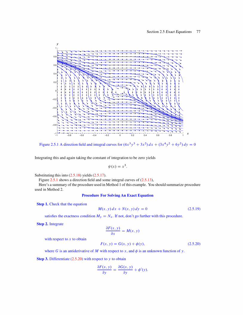
Section 2.5 Exact Equations 77
!1 !0.8 !0.6 !0.4 !0.2 0 0.2 0.4 0.6 0.8 1!1
!0.8
!0.6
!0.4
!0.2
0
0.2
0.4
0.6
0.8
1
y
x
Figure 2.5.1 A direction field and integral curves for .4x3y3 C 3x2/ dx C .3x4y2 C 6y2/ dy D 0
Integrating this and again taking the constant of integration to be zero yields
.x/ D x3:
Substituting this into (2.5.18) yields (2.5.17).Figure 2.5.1 shows a direction field and some integral curves of (2.5.13),Here’s a summary of the procedure used in Method 1 of this example. You should summarize procedure
used in Method 2.
Procedure For Solving An Exact Equation
Step 1. Check that the equationM.x; y/ dx CN.x; y/ dy D 0 (2.5.19)
satisfies the exactness conditionMy D Nx. If not, don’t go further with this procedure.
Step 2. [email protected]; y/
@xD M.x; y/
with respect to x to obtainF.x; y/ D G.x; y/C !.y/; (2.5.20)
where G is an antiderivative of M with respect to x, and ! is an unknown function of y.
Step 3. Differentiate (2.5.20) with respect to y to obtain
@F.x; y/
@[email protected]; y/
@yC !0.y/:
78 Chapter 2 First Order Equations
Step 4. Equate the right side of this equation to N and solve for !0; thus,
@G.x; y/
@yC !0.y/ D N.x; y/; so !0.y/ D N.x; y/ !
@G.x; y/
@y:
Step 5. Integrate !0 with respect to y, taking the constant of integration to be zero, and substitute theresult in (2.5.20) to obtain F.x; y/.
Step 6. Set F.x; y/ D c to obtain an implicit solution of (2.5.19). If possible, solve for y explicitly asa function of x.
It’s a common mistake to omit Step 6. However, it’s important to include this step, since F isn’t itselfa solution of (2.5.19).
Many equations can be conveniently solved by either of the two methods used in Example 2.5.3. How-ever, sometimes the integration required in one approach is more difficult than in the other. In such caseswe choose the approach that requires the easier integration.
Example 2.5.4 Solve the equation
.yexy tan x C exy sec2 x/ dx C xexy tan x dy D 0: (2.5.21)
Solution We leave it to you to check that My D Nx on any open rectangle where tan x and sec x aredefined. Here we must find a function F such that
Fx.x; y/ D yexy tanx C exy sec2 x (2.5.22)
andFy.x; y/ D xexy tan x: (2.5.23)
It’s difficult to integrate (2.5.22) with respect to x, but easy to integrate (2.5.23) with respect to y. Thisyields
F.x; y/ D exy tanx C .x/: (2.5.24)
Differentiating this with respect to x yields
Fx.x; y/ D yexy tanx C exy sec2 x C 0.x/:
Comparing this with (2.5.22) shows that 0.x/ D 0. Hence, is a constant, which we can take to bezero in (2.5.24), and
exy tanx D c
is an implicit solution of (2.5.21).Attempting to apply our procedure to an equation that isn’t exact will lead to failure in Step 4, since
the function
N !@G
@y
won’t be independent of x if My ¤ Nx (Exercise 31), and therefore can’t be the derivative of a functionof y alone. Here’s an example that illustrates this.
Example 2.5.5 Verify that the equation
3x2y2 dx C 6x3y dy D 0 (2.5.25)
is not exact, and show that the procedure for solving exact equations fails when applied to (2.5.25).
Section 2.5 Exact Equations 79
Solution HereMy.x; y/ D 6x2y and Nx.x; y/ D 18x2y;
so (2.5.25) isn’t exact. Nevertheless, let’s try to find a function F such that
Fx.x; y/ D 3x2y2 (2.5.26)
andFy.x; y/ D 6x3y: (2.5.27)
Integrating (2.5.26) with respect to x yields
F.x; y/ D x3y2 C !.y/;
and differentiating this with respect to y yields
Fy.x; y/ D 2x3y C !0.y/:
For this equation to be consistent with (2.5.27),
6x3y D 2x3y C !0.y/;
or!0.y/ D 4x3y:
This is a contradiction, since !0 must be independent of x. Therefore the procedure fails.
2.5 Exercises
In Exercises 1–17 determine which equations are exact and solve them.
1. 6x2y2 dx C 4x3y dy D 0
2. .3y cos x C 4xex C 2x2ex/ dx C .3 sinx C 3/ dy D 0
3. 14x2y3 dx C 21x2y2 dy D 0
4. .2x ! 2y2/ dx C .12y2 ! 4xy/ dy D 0
5. .x C y/2 dx C .x C y/2 dy D 0 6. .4x C 7y/ dx C .3x C 4y/ dy D 0
7. .!2y2 sin x C 3y3 ! 2x/ dx C .4y cos x C 9xy2/ dy D 0
8. .2x C y/ dx C .2y C 2x/ dy D 0
9. .3x2 C 2xy C 4y2/ dx C .x2 C 8xy C 18y/ dy D 0
10. .2x2 C 8xy C y2/ dx C .2x2 C xy3=3/ dy D 0
11.
!
1
xC 2x
"
dx C!
1
yC 2y
"
dy D 0
12. .y sinxy C xy2 cos xy/ dx C .x sinxy C xy2 cos xy/ dy D 0
13.x dx
.x2 C y2/3=2C
y dy
.x2 C y2/3=2D 0
14.#
ex.x2y2 C 2xy2/C 6x$
dx C .2x2yex C 2/ dy D 0
15.%
x2ex2Cy .2x2 C 3/C 4x&
dx C .x3ex2Cy ! 12y2/ dy D 0

80 Chapter 2 First Order Equations
16.!
exy.x4y C 4x3/C 3y"
dx C .x5exy C 3x/ dy D 0
17. .3x2 cos xy ! x3y sinxy C 4x/ dx C .8y ! x4 sinxy/ dy D 0
In Exercises 18–22 solve the initial value problem.
18. .4x3y2 ! 6x2y ! 2x ! 3/ dx C .2x4y ! 2x3/ dy D 0; y.1/ D 3
19. .!4y cos x C 4 sinx cos x C sec2 x/ dx C .4y ! 4 sinx/ dy D 0; y.!=4/ D 0
20. .y3 ! 1/ex dx C 3y2.ex C 1/ dy D 0; y.0/ D 0
21. .sinx ! y sin x ! 2 cos x/ dx C cos x dy D 0; y.0/ D 1
22. .2x ! 1/.y ! 1/ dx C .x C 2/.x ! 3/ dy D 0; y.1/ D !1
23. C/G Solve the exact equation
.7x C 4y/ dx C .4x C 3y/ dy D 0:
Plot a direction field and some integral curves for this equation on the rectangle
f!1 " x " 1;!1 " y " 1g:
24. C/G Solve the exact equation
ex.x4y2 C 4x3y2 C 1/ dx C .2x4yex C 2y/ dy D 0:
Plot a direction field and some integral curves for this equation on the rectangle
f!2 " x " 2;!1 " y " 1g:
25. C/G Plot a direction field and some integral curves for the exact equation
.x3y4 C x/ dx C .x4y3 C y/ dy D 0
on the rectangle f!1 " x " 1;!1 " y " 1g. (See Exercise 37(a)).
26. C/G Plot a direction field and some integral curves for the exact equation
.3x2 C 2y/ dx C .2y C 2x/ dy D 0
on the rectangle f!2 " x " 2;!2 " y " 2g. (See Exercise 37(b)).
27. L
(a) Solve the exact equation
.x3y4 C 2x/ dx C .x4y3 C 3y/ dy D 0 .A/
implicitly.
(b) For what choices of .x0; y0/ does Theorem 2.3.1 imply that the initial value problem
.x3y4 C 2x/ dx C .x4y3 C 3y/ dy D 0; y.x0/ D y0; .B/
has a unique solution on an open interval .a; b/ that contains x0?
Section 2.5 Exact Equations 81
(c) Plot a direction field and some integral curves for (A) on a rectangular region centered at theorigin. What is the interval of validity of the solution of (B)?
28. L
(a) Solve the exact equation.x2 C y2/ dx C 2xy dy D 0 .A/
implicitly.
(b) For what choices of .x0; y0/ does Theorem 2.3.1 imply that the initial value problem
.x2 C y2/ dx C 2xy dy D 0; y.x0/ D y0; .B/
has a unique solution y D y.x/ on some open interval .a; b/ that contains x0?
(c) Plot a direction field and some integral curves for (A). From the plot determine, the interval.a; b/ of (b), the monotonicity properties (if any) of the solution of (B), and limx!aC y.x/and limx!b! y.x/. HINT: Your answers will depend upon which quadrant contains .x0; y0/.
29. Find all functionsM such that the equation is exact.
(a) M.x; y/ dx C .x2 ! y2/ dy D 0
(b) M.x; y/ dx C 2xy sinx cosy dy D 0
(c) M.x; y/ dx C .ex ! ey sinx/ dy D 0
30. Find all functionsN such that the equation is exact.
(a) .x3y2 C 2xy C 3y2/ dx CN.x; y/ dy D 0
(b) .ln xy C 2y sinx/ dx CN.x; y/ dy D 0
(c) .x sinx C y siny/ dx CN.x; y/ dy D 0
31. Suppose M;N; and their partial derivatives are continuous on an open rectangle R, and G is anantiderivative of M with respect to x; that is,
@G
@xD M:
Show that if My ¤ Nx inR then the function
N !@G
@y
is not independent of x.
32. Prove: If the equations M1 dx C N1 dy D 0 and M2 dx C N2 dy D 0 are exact on an openrectangle R, so is the equation
.M1 CM2/ dx C .N1 CN2/ dy D 0:
33. Find conditions on the constants A, B , C , and D such that the equation
.Ax C By/dx C .Cx CDy/dy D 0
is exact.
34. Find conditions on the constants A, B , C , D, E , and F such that the equation
.Ax2 C Bxy C Cy2/ dx C .Dx2 C Exy C Fy2/ dy D 0
is exact.
82 Chapter 2 First Order Equations
35. SupposeM and N are continuous and have continuous partial derivatives My and Nx that satisfythe exactness conditionMy D Nx on an open rectangle R. Show that if .x; y/ is in R and
F.x; y/ DZ x
x0
M.s; y0/ ds CZ y
y0
N.x; t/ dt;
then Fx D M and Fy D N .
36. Under the assumptions of Exercise 35, show that
F.x; y/ DZ y
y0
N.x0; s/ ds CZ x
x0
M.t; y/ dt:
37. Use the method suggested by Exercise 35, with .x0; y0/ D .0; 0/, to solve the these exact equa-tions:
(a) .x3y4 C x/ dx C .x4y3 C y/ dy D 0
(b) .x2 C y2/ dx C 2xy dy D 0
(c) .3x2 C 2y/ dx C .2y C 2x/ dy D 0
38. Solve the initial value problem
y0 C2
xy D !
2xy
x2 C 2x2y C 1; y.1/ D !2:
39. Solve the initial value problem
y0 !3
xy D
2x4.4x3 ! 3y/3x5 C 3x3 C 2y
; y.1/ D 1:
40. Solve the initial value problem
y0 C 2xy D !e!x2
3x C 2yex2
2x C 3yex2
!
; y.0/ D !1:
41. Rewrite the separable equationh.y/y0 D g.x/ .A/
as an exact equationM.x; y/ dx CN.x; y/ dy D 0: .B/
Show that applying the method of this section to (B) yields the same solutions that would beobtained by applying the method of separation of variables to (A)
42. Suppose all second partial derivatives of M D M.x; y/ and N D N.x; y/ are continuous andM dx C N dy D 0 and !N dx C M dy D 0 are exact on an open rectangle R. Show thatMxx CMyy D Nxx CNyy D 0 on R.
43. Suppose all second partial derivatives of F D F.x; y/ are continuous and Fxx C Fyy D 0 on anopen rectangle R. (A function with these properties is said to be harmonic; see also Exercise 42.)Show that !Fy dx C Fx dy D 0 is exact on R, and therefore there’s a function G such thatGx D !Fy and Gy D Fx in R. (A function G with this property is said to be a harmonic
conjugate of F .)
Section 2.6 Exact Equations 83
44. Verify that the following functions are harmonic, and find all their harmonic conjugates. (SeeExercise 43.)
(a) x2 ! y2 (b) ex cosy (c) x3 ! 3xy2
(d) cos x cosh y (e) sinx cosh y
2.6 INTEGRATING FACTORS
In Section 2.5 we saw that if M , N , My and Nx are continuous and My D Nx on an open rectangle Rthen
M.x; y/ dx CN.x; y/ dy D 0 (2.6.1)
is exact on R. Sometimes an equation that isn’t exact can be made exact by multiplying it by an appro-priate function. For example,
.3x C 2y2/ dx C 2xy dy D 0 (2.6.2)
is not exact, sinceMy .x; y/ D 4y ¤ Nx.x; y/ D 2y in (2.6.2). However, multiplying (2.6.2) by x yields
.3x2 C 2xy2/ dx C 2x2y dy D 0; (2.6.3)
which is exact, since My.x; y/ D Nx.x; y/ D 4xy in (2.6.3). Solving (2.6.3) by the procedure given inSection 2.5 yields the implicit solution
x3 C x2y2 D c:
A function ! D !.x; y/ is an integrating factor for (2.6.1) if
!.x; y/M.x; y/ dx C !.x; y/N.x; y/ dy D 0 (2.6.4)
is exact. If we know an integrating factor ! for (2.6.1), we can solve the exact equation (2.6.4) by themethod of Section 2.5. It would be nice if we could say that (2.6.1) and (2.6.4) always have the samesolutions, but this isn’t so. For example, a solution y D y.x/ of (2.6.4) such that !.x; y.x// D 0 onsome interval a < x < b could fail to be a solution of (2.6.1) (Exercise 1), while (2.6.1) may have asolution y D y.x/ such that !.x; y.x// isn’t even defined (Exercise 2). Similar comments apply if y isthe independent variable and x is the dependent variable in (2.6.1) and (2.6.4). However, if !.x; y/ isdefined and nonzero for all .x; y/, (2.6.1) and (2.6.4) are equivalent; that is, they have the same solutions.
Finding Integrating Factors
By applying Theorem 2.5.2 (withM and N replaced by !M and !N ), we see that (2.6.4) is exact on anopen rectangle R if !M , !N , .!M/y , and .!N/x are continuous and
@
@y.!M/ D
@
@x.!N/ or, equivalently, !yM C !My D !xN C !Nx
on R. It’s better to rewrite the last equation as
!.My ! Nx/ D !xN ! !yM; (2.6.5)
which reduces to the known result for exact equations; that is, ifMy D Nx then (2.6.5) holds with! D 1,so (2.6.1) is exact.
You may think (2.6.5) is of little value, since it involves partial derivatives of the unknown integratingfactor !, and we haven’t studied methods for solving such equations. However, we’ll now show that
84 Chapter 2 Integrating Factors
(2.6.5) is useful if we restrict our search to integrating factors that are products of a function of x and afunction of y; that is, !.x; y/ D P.x/Q.y/. We’re not saying that every equation M dx C N dy D 0has an integrating factor of this form; rather, we’re saying that some equations have such integratingfactors.We’llnow develop a way to determine whether a given equation has such an integrating factor,and a method for finding the integrating factor in this case.
If !.x; y/ D P.x/Q.y/, then !x.x; y/ D P 0.x/Q.y/ and !y.x; y/ D P.x/Q0.y/, so (2.6.5) be-comes
P.x/Q.y/.My ! Nx/ D P 0.x/Q.y/N ! P.x/Q0.y/M; (2.6.6)
or, after dividing through by P.x/Q.y/,
My !Nx DP 0.x/
P.x/N !
Q0.y/
Q.y/M: (2.6.7)
Now let
p.x/ DP 0.x/
P.x/and q.y/ D
Q0.y/
Q.y/;
so (2.6.7) becomesMy !Nx D p.x/N ! q.y/M: (2.6.8)
We obtained (2.6.8) by assuming that M dx C N dy D 0 has an integrating factor !.x; y/ DP.x/Q.y/. However, we can now view (2.6.7) differently: If there are functionsp D p.x/ and q D q.y/that satisfy (2.6.8) and we define
P.x/ D ˙eR
p.x/ dx and Q.y/ D ˙eR
q.y/ dy ; (2.6.9)
then reversing the steps that led from (2.6.6) to (2.6.8) shows that !.x; y/ D P.x/Q.y/ is an integratingfactor for M dx C N dy D 0. In using this result, we take the constants of integration in (2.6.9) to bezero and choose the signs conveniently so the integrating factor has the simplest form.
There’s no simple general method for ascertaining whether functions p D p.x/ and q D q.y/ satisfy-ing (2.6.8) exist. However, the next theorem gives simple sufficient conditions for the given equation tohave an integrating factor that depends on only one of the independent variables x and y, and for findingan integrating factor in this case.
Theorem 2.6.1 Let M; N; My ; and Nx be continuous on an open rectangle R: ThenW(a) If .My ! Nx/=N is independent of y on R and we define
p.x/ DMy !Nx
N
then
!.x/ D ˙eR
p.x/ dx (2.6.10)
is an integrating factor for
M.x; y/ dx CN.x; y/ dy D 0 (2.6.11)
on R:
(b) If .Nx !My/=M is independent of x on R and we define
q.y/ DNx !My
M;
then
!.y/ D ˙eR
q.y/ dy (2.6.12)
is an integrating factor for (2.6.11) on R:
Section 2.6 Exact Equations 85
Proof (a) If .My !Nx/=N is independent of y, then (2.6.8) holds with p D .My !Nx/=N and q " 0.Therefore
P.x/ D ˙eR
p.x/ dx and Q.y/ D ˙eR
q.y/ dy D ˙e0 D ˙1;
so (2.6.10) is an integrating factor for (2.6.11) on R.(b) If .Nx !My /=M is independent of x then eqrefeq:2.6.8 holds withp " 0 and q D .Nx !My /=M ,
and a similar argument shows that (2.6.12) is an integrating factor for (2.6.11) on R.The next two examples show how to apply Theorem 2.6.1.
Example 2.6.1 Find an integrating factor for the equation
.2xy3 ! 2x3y3 ! 4xy2 C 2x/ dx C .3x2y2 C 4y/ dy D 0 (2.6.13)
and solve the equation.
Solution In (2.6.13)
M D 2xy3 ! 2x3y3 ! 4xy2 C 2x; N D 3x2y2 C 4y;
andMy ! Nx D .6xy2 ! 6x3y2 ! 8xy/ ! 6xy2 D !6x3y2 ! 8xy;
so (2.6.13) isn’t exact. However,
My !Nx
ND !
6x3y2 C 8xy
3x2y2 C 4yD !2x
is independent of y, so Theorem 2.6.1(a) applies with p.x/ D !2x. SinceZ
p.x/ dx D !Z
2x dx D !x2;
!.x/ D e!x2is an integrating factor. Multiplying (2.6.13) by ! yields the exact equation
e!x2.2xy3 ! 2x3y3 ! 4xy2 C 2x/ dx C e!x2
.3x2y2 C 4y/ dy D 0: (2.6.14)
To solve this equation, we must find a function F such that
Fx.x; y/ D e!x2
.2xy3 ! 2x3y3 ! 4xy2 C 2x/ (2.6.15)
andFy.x; y/ D e!x2
.3x2y2 C 4y/: (2.6.16)
Integrating (2.6.16) with respect to y yields
F.x; y/ D e!x2
.x2y3 C 2y2/C .x/: (2.6.17)
Differentiating this with respect to x yields
Fx.x; y/ D e!x2
.2xy3 ! 2x3y3 ! 4xy2/C 0.x/:
Comparing this with (2.6.15) shows that 0.x/ D 2xe!x2; therefore, we can let .x/ D !e!x2
in(2.6.17) and conclude that
e!x2 !
y2.x2y C 2/ ! 1"
D c
is an implicit solution of (2.6.14). It is also an implicit solution of (2.6.13).Figure 2.6.1 shows a direction field and some integal curves for (2.6.13)

86 Chapter 2 Integrating Factors
!2 !1.5 !1 !0.5 0 0.5 1 1.5 2!4
!3
!2
!1
0
1
2
3
4
y
x
Figure 2.6.1 A direction field and integral curves for.2xy3 ! 2x3y3 ! 4xy2 C 2x/ dx C .3x2y2 C 4y/ dy D 0
Example 2.6.2 Find an integrating factor for
2xy3 dx C .3x2y2 C x2y3 C 1/ dy D 0 (2.6.18)
and solve the equation.
Solution In (2.6.18),M D 2xy3; N D 3x2y2 C x2y3 C 1;
andMy ! Nx D 6xy2 ! .6xy2 C 2xy3/ D !2xy3;
so (2.6.18) isn’t exact. Moreover,
My !Nx
ND !
2xy3
3x2y2 C x2y2 C 1
is not independent of y, so Theorem 2.6.1(a) does not apply. However, Theorem 2.6.1(b) does apply,since
Nx !My
MD2xy3
2xy3D 1
is independent of x, so we can take q.y/ D 1. Since
Z
q.y/ dy DZ
dy D y;
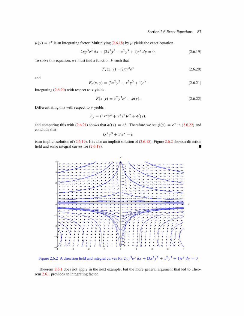
Section 2.6 Exact Equations 87
!.y/ D ey is an integrating factor. Multiplying (2.6.18) by ! yields the exact equation
2xy3ey dx C .3x2y2 C x2y3 C 1/ey dy D 0: (2.6.19)
To solve this equation, we must find a functionF such that
Fx.x; y/ D 2xy3ey (2.6.20)
andFy.x; y/ D .3x2y2 C x2y3 C 1/ey : (2.6.21)
Integrating (2.6.20) with respect to x yields
F.x; y/ D x2y3ey C ".y/: (2.6.22)
Differentiating this with respect to y yields
Fy D .3x2y2 C x2y3/ey C "0.y/;
and comparing this with (2.6.21) shows that "0.y/ D ey . Therefore we set ".y/ D ey in (2.6.22) andconclude that
.x2y3 C 1/ey D c
is an implicit solution of (2.6.19). It is also an implicit solution of (2.6.18). Figure 2.6.2 shows a directionfield and some integral curves for (2.6.18).
!4 !3 !2 !1 0 1 2 3 4!4
!3
!2
!1
0
1
2
3
4
y
x
Figure 2.6.2 A direction field and integral curves for 2xy3ey dx C .3x2y2 C x2y3 C 1/ey dy D 0
Theorem 2.6.1 does not apply in the next example, but the more general argument that led to Theo-rem 2.6.1 provides an integrating factor.
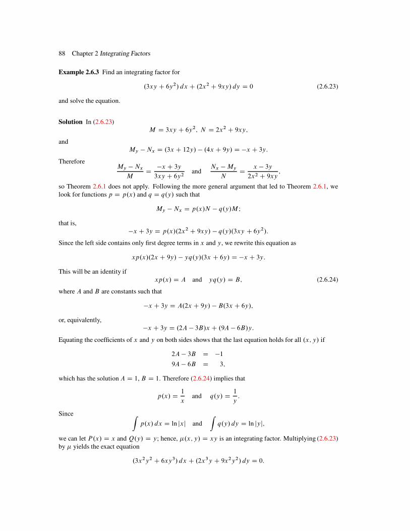
88 Chapter 2 Integrating Factors
Example 2.6.3 Find an integrating factor for
.3xy C 6y2/ dx C .2x2 C 9xy/ dy D 0 (2.6.23)
and solve the equation.
Solution In (2.6.23)M D 3xy C 6y2; N D 2x2 C 9xy;
andMy !Nx D .3x C 12y/ ! .4x C 9y/ D !x C 3y:
ThereforeMy ! Nx
MD
!x C 3y
3xy C 6y2and
Nx !My
ND
x ! 3y
2x2 C 9xy;
so Theorem 2.6.1 does not apply. Following the more general argument that led to Theorem 2.6.1, welook for functions p D p.x/ and q D q.y/ such that
My ! Nx D p.x/N ! q.y/M I
that is,!x C 3y D p.x/.2x2 C 9xy/ ! q.y/.3xy C 6y2/:
Since the left side contains only first degree terms in x and y, we rewrite this equation as
xp.x/.2x C 9y/ ! yq.y/.3x C 6y/ D !x C 3y:
This will be an identity ifxp.x/ D A and yq.y/ D B; (2.6.24)
where A and B are constants such that
!x C 3y D A.2x C 9y/ ! B.3x C 6y/;
or, equivalently,!x C 3y D .2A ! 3B/x C .9A ! 6B/y:
Equating the coefficients of x and y on both sides shows that the last equation holds for all .x; y/ if
2A! 3B D !19A! 6B D 3;
which has the solutionA D 1, B D 1. Therefore (2.6.24) implies that
p.x/ D1
xand q.y/ D
1
y:
SinceZ
p.x/ dx D ln jxj and
Z
q.y/ dy D ln jyj;
we can let P.x/ D x and Q.y/ D y; hence, !.x; y/ D xy is an integrating factor. Multiplying (2.6.23)by ! yields the exact equation
.3x2y2 C 6xy3/ dx C .2x3y C 9x2y2/ dy D 0:
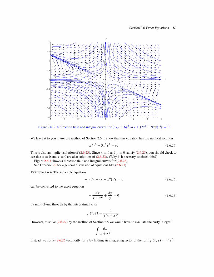
Section 2.6 Exact Equations 89
!4 !3 !2 !1 0 1 2 3 4!2
!1.5
!1
!0.5
0
0.5
1
1.5
2
y
x
Figure 2.6.3 A direction field and integral curves for .3xy C 6y2/ dx C .2x2 C 9xy/ dy D 0
We leave it to you to use the method of Section 2.5 to show that this equation has the implicit solution
x3y2 C 3x2y3 D c: (2.6.25)
This is also an implicit solution of (2.6.23). Since x ! 0 and y ! 0 satisfy (2.6.25), you should check tosee that x ! 0 and y ! 0 are also solutions of (2.6.23). (Why is it necesary to check this?)
Figure 2.6.3 shows a direction field and integral curves for (2.6.23).See Exercise 28 for a general discussion of equations like (2.6.23).
Example 2.6.4 The separable equation
" y dx C .x C x6/ dy D 0 (2.6.26)
can be converted to the exact equation
"dx
x C x6Cdy
yD 0 (2.6.27)
by multiplying through by the integrating factor
!.x; y/ D1
y.x C x6/:
However, to solve (2.6.27) by the method of Section 2.5 we would have to evaluate the nasty integralZ
dx
x C x6:
Instead, we solve (2.6.26) explicitly for y by finding an integrating factor of the form !.x; y/ D xayb .
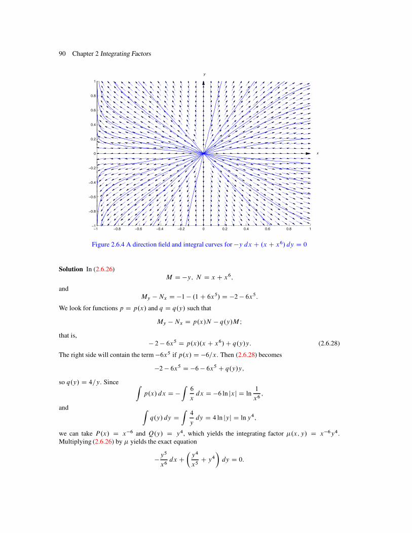
90 Chapter 2 Integrating Factors
!1 !0.8 !0.6 !0.4 !0.2 0 0.2 0.4 0.6 0.8 1!1
!0.8
!0.6
!0.4
!0.2
0
0.2
0.4
0.6
0.8
1
y
x
Figure 2.6.4 A direction field and integral curves for !y dx C .x C x6/ dy D 0
Solution In (2.6.26)M D !y; N D x C x6;
andMy !Nx D !1 ! .1 C 6x5/ D !2 ! 6x5:
We look for functions p D p.x/ and q D q.y/ such that
My ! Nx D p.x/N ! q.y/M I
that is,! 2 ! 6x5 D p.x/.x C x6/C q.y/y: (2.6.28)
The right side will contain the term !6x5 if p.x/ D !6=x. Then (2.6.28) becomes
!2 ! 6x5 D !6 ! 6x5 C q.y/y;
so q.y/ D 4=y. SinceZ
p.x/ dx D !Z
6
xdx D !6 ln jxj D ln
1
x6;
andZ
q.y/ dy DZ
4
ydy D 4 ln jyj D lny4;
we can take P.x/ D x!6 and Q.y/ D y4, which yields the integrating factor !.x; y/ D x!6y4.Multiplying (2.6.26) by ! yields the exact equation
!y5
x6dx C
!
y4
x5C y4
"
dy D 0:
Section 2.6 Exact Equations 91
We leave it to you to use the method of the Section 2.5 to show that this equation has the implicit solution!y
x
"5C y5 D k:
Solving for y yieldsy D k1=5x.1C x5/!1=5;
which we rewrite asy D cx.1C x5/!1=5
by renaming the arbitrary constant. This is also a solution of (2.6.26).Figure 2.6.4 shows a direction field and some integral curves for (2.6.26).
2.6 Exercises
1. (a) Verify that !.x; y/ D y is an integrating factor for
y dx C#
2x C1
y
$
dy D 0 .A/
on any open rectangle that does not intersect the x axis or, equivalently, that
y2 dx C .2xy C 1/ dy D 0 .B/
is exact on any such rectangle.
(b) Verify that y ! 0 is a solution of (B), but not of (A).
(c) Show thaty.xy C 1/ D c .C/
is an implicit solution of (B), and explain why every differentiable function y D y.x/ otherthan y ! 0 that satisfies (C) is also a solution of (A).
2. (a) Verify that !.x; y/ D 1=.x " y/2 is an integrating factor for
"y2 dx C x2 dy D 0 .A/
on any open rectangle that does not intersect the line y D x or, equivalently, that
"y2
.x " y/2dx C
x2
.x " y/2dy D 0 .B/
is exact on any such rectangle.
(b) Use Theorem 2.2.1 to show thatxy
.x " y/D c .C/
is an implicit solution of (B), and explain why it’s also an implicit solution of (A)
(c) Verify that y D x is a solution of (A), even though it can’t be obtained from (C).
In Exercises 3–16 find an integrating factor; that is a function of only one variable, and solve the given
equation.
3. y dx " x dy D 0 4. 3x2y dx C 2x3 dy D 0
5. 2y3 dx C 3y2 dy D 0 6. .5xy C 2y C 5/ dx C 2x dy D 0
92 Chapter 2 Integrating Factors
7. .xy C x C 2y C 1/ dx C .x C 1/ dy D 0
8. .27xy2 C 8y3/ dx C .18x2y C 12xy2/ dy D 0
9. .6xy2 C 2y/ dx C .12x2y C 6x C 3/ dy D 0
10. y2 dx C!
xy2 C 3xy C1
y
"
dy D 0
11. .12x3y C 24x2y2/ dx C .9x4 C 32x3y C 4y/ dy D 0
12. .x2y C 4xy C 2y/ dx C .x2 C x/ dy D 0
13. !y dx C .x4 ! x/ dy D 0
14. cos x cosy dx C .sin x cosy ! sinx sin y C y/ dy D 0
15. .2xy C y2/ dx C .2xy C x2 ! 2x2y2 ! 2xy3/ dy D 0
16. y siny dx C x.siny ! y cosy/ dy D 0
In Exercises 17–23 find an integrating factor of the form !.x; y/ D P.x/Q.y/ and solve the given
equation.
17. y.1 C 5 ln jxj/ dx C 4x ln jxj dy D 0
18. .˛y C "xy/ dx C .ˇx C ıxy/ dy D 0
19. .3x2y3 ! y2 C y/ dx C .!xy C 2x/ dy D 0
20. 2y dx C 3.x2 C x2y3/ dy D 0
21. .a cos xy ! y sinxy/ dx C .b cos xy ! x sinxy/ dy D 0
22. x4y4 dx C x5y3 dy D 0
23. y.x cos x C 2 sinx/ dx C x.y C 1/ sinx dy D 0
In Exercises 24–27 find an integrating factor and solve the equation. Plot a direction field and some
integral curves for the equation in the indicated rectangular region.
24. C/G .x4y3 C y/ dx C .x5y2 ! x/ dy D 0I f!1 " x " 1;!1 " y " 1g
25. C/G .3xy C 2y2 C y/ dx C .x2 C 2xy C x C 2y/ dy D 0I f!2 " x " 2;!2 " y " 2g
26. C/G .12xy C 6y3/ dx C .9x2 C 10xy2/ dy D 0I f!2 " x " 2;!2 " y " 2g
27. C/G .3x2y2 C 2y/ dx C 2x dy D 0I f!4 " x " 4;!4 " y " 4g28. Suppose a, b, c, and d are constants such that ad ! bc ¤ 0, and let m and n be arbitrary real
numbers. Show that
.axmy C bynC1/ dx C .cxmC1 C dxyn/ dy D 0
has an integrating factor !.x; y/ D x˛yˇ .
29. Suppose M , N , Mx , and Ny are continuous for all .x; y/, and ! D !.x; y/ is an integratingfactor for
M.x; y/ dx CN.x; y/ dy D 0: .A/
Assume that !x and !y are continuous for all .x; y/, and suppose y D y.x/ is a differentiablefunction such that !.x; y.x// D 0 and !x.x; y.x// ¤ 0 for all x in some interval I . Show that yis a solution of (A) on I .
Section 2.6 Exact Equations 93
30. According to Theorem 2.1.2, the general solution of the linear nonhomogeneous equation
y0 C p.x/y D f .x/ .A/
is
y D y1.x/
!
c CZ
f .x/=y1.x/ dx
"
; .B/
where y1 is any nontrivial solution of the complementary equation y0 C p.x/y D 0. In thisexercise we obtain this conclusion in a different way. You may find it instructive to apply themethod suggested here to solve some of the exercises in Section 2.1.
(a) Rewrite (A) asŒp.x/y ! f .x/! dx C dy D 0; .C/
and show that " D ˙eR
p.x/ dx is an integrating factor for (C).
(b) Multiply (A) through by " D ˙eR
p.x/ dx and verify that the resulting equation can berewritten as
.".x/y/0 D ".x/f .x/:
Then integrate both sides of this equation and solve for y to show that the general solutionof (A) is
y D1
".x/
!
c CZ
f .x/".x/ dx
"
:
Why is this form of the general solution equivalent to (B)?