Embed Size (px)
Citation preview

UNIT1
Introduction
Algorithm
• An Algorithm is a sequence of unambiguous instructions for solving a problem,
• i.e., for obtaining a required output for any legitimate input in a finite amount of time.

Notion of algorithm
“computer”
Algorithmic solution
problem
algorithm
input output

PSEUDOCODE Pseudocode (pronounced SOO-doh-kohd) is a detailed yet
readable description of what a computer program or algorithm must do, expressed in a formally-styled natural language rather than in a programming language.
It is sometimes used as a detailed step in the process of
developing a program. It allows programmers to express the design in great detail
and provides programmers a detailed template for the next step of writing code in a specific programming language.

Formatting and Conventions in Pseudocoding
INDENTATION in pseudocode should be identical to its implementation in a programming language. Try to indent at least four spaces.
The pseudocode entries are to be cryptic, AND SHOULD NOT BE PROSE. NO SENTENCES.
No flower boxes in pseudocode. Do not include data declarations in
pseudocode.

Some Keywords That Should be Used
• For looping and selection,
Do While...EndDo;
– Do Until...Enddo;
– Case...EndCase;
– If...Endif;
– Call ... with (parameters); Call; Return ....; Return; When; Always use scope terminators for loops and iteration.

Some Keywords …
• As verbs, use the words
– generate, Compute, Process,
– Set, reset,
– increment,
– calculate,
– add, sum, multiply, ...
– print, display,
– input, output, edit, test , etc.

Methods of finding GCD
M - 1
M - 2
M - 3

Fundamentals of Analysis of
algorithm efficiency

Analysis of algorithms
Issues:
correctness
time efficiency
space efficiency
optimality
Approaches:
theoretical analysis
empirical analysis

Theoretical analysis of time efficiency
Time efficiency is analyzed by determining the number of repetitions of the basic operation as a function of input size
Basic operation: the operation that contributes the most towards the running time of the algorithm
T(n) ≈ copC(n) running time execution time
for basic operation
or cost
Number of times
basic operation is
executed
input size
Note: Different basic operations may cost differently!
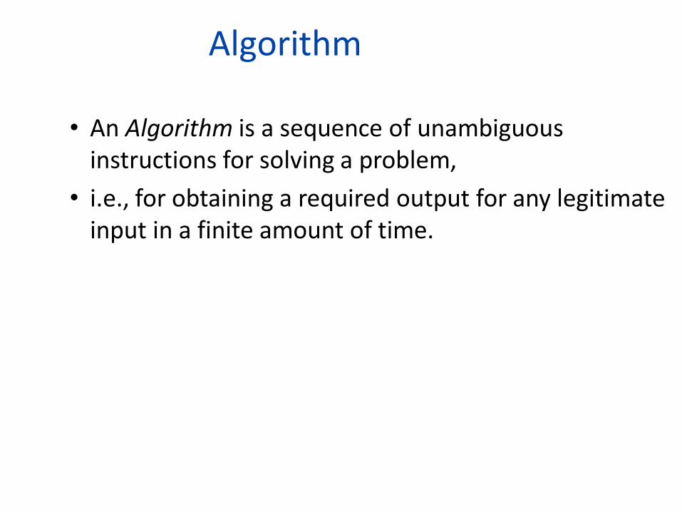
Input size and basic operation examples
Problem Input size measure Basic operation
Searching for key
in a list of n items
Number of list’s
items, i.e. n Key comparison
Multiplication of
two matrices
Matrix dimensions or
total number of
elements
Multiplication of
two numbers
Checking primality
of a given integer n
n’size = number of
digits (in binary
representation)
Division
Typical graph
problem
#vertices and/or
edges
Visiting a vertex
or traversing an
edge

Empirical analysis of time efficiency
Select a specific (typical) sample of inputs
Use physical unit of time (e.g., milliseconds) or Count actual number of basic operation’s
executions
Analyze the empirical data

Efficiencies
Worst Case Efficiency:
Is its efficiency for the worst case input of size n, which is an input of size n for which the algorithm runs the longest among all possible inputs of that size
Cworst(n)
Best-case efficiency:
Is its efficiency for the worst case input of size n, which is an input of size n for which the algorithm runs the fastest among all possible inputs of that size
Cbest(n)

Amortized efficiency
– It applies not to a single run of an algorithm, but rather to a sequence of operations performed on the same data structure

Best-case, average-case, worst-case
For some algorithms, efficiency depends on form of input: Worst case: Cworst(n) – maximum over inputs of size n Best case: Cbest(n) – minimum over inputs of size n Average case: Cavg(n) – “average” over inputs of size n Number of times the basic operation will be executed on
typical input
NOT the average of worst and best case
Expected number of basic operations considered as a random variable under some assumption about the probability distribution of all possible inputs. So, avg = expected under uniform distribution.

Example: Sequential search
Worst case
Best case
Average case
n key comparisons
1 comparisons
(n+1)/2, assuming K is in A

Types of formulas for basic operation’s count
Exact formula e.g., C(n) = n(n-1)/2
Formula indicating order of growth with
specific multiplicative constant e.g., C(n) ≈ 0.5 n2
Formula indicating order of growth with
unknown multiplicative constant e.g., C(n) ≈ cn2

Order of growth • Most important: Order of growth within a
constant multiple as n→∞
• Example:
– How much faster will algorithm run on computer that is twice as fast?
– How much longer does it take to solve problem of double input size?

Values of some important functions as n

Asymptotic Notations
• O (Big-Oh)-notation
• Ω (Big-Omega) -notation
• Θ (Big-Theta) -notation

Asymptotic order of growth A way of comparing functions that ignores constant
factors and small input sizes (because?)
O(g(n)): class of functions f(n) that grow no faster than g(n)
Θ(g(n)): class of functions f(n) that grow at same rate as g(n)
Ω(g(n)): class of functions f(n) that grow at least as fast as g(n)

O-notation
Definition: A function t(n) is said to be in O(g(n)), denoted t(n) O(g(n)) is bounded above by some constant multiple of g(n) for all large n, i.e., there exist positive constant c and non-negative integer n0 such that
f(n) ≤ c g(n) for every n ≥ n0

Big-oh

-notation
• Formal definition – A function t(n) is said to be in (g(n)), denoted
t(n) (g(n)), if t(n) is bounded below by some constant multiple of g(n) for all large n, i.e., if there exist some positive constant c and some nonnegative integer n0 such that
t(n) cg(n) for all n n0

Big-omega

-notation
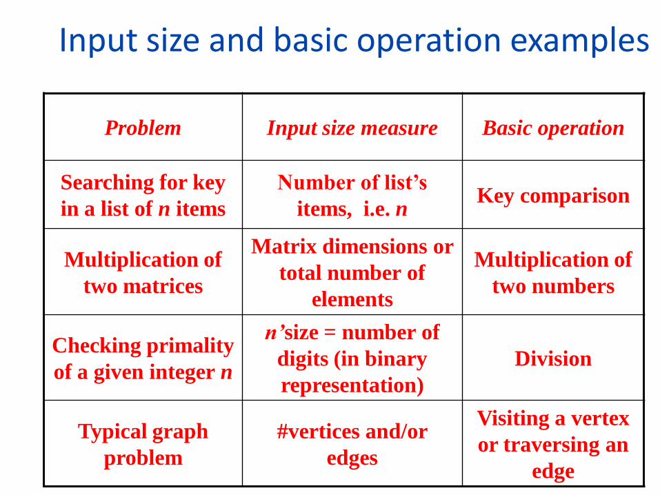
• Formal definition – A function t(n) is said to be in (g(n)), denoted
t(n) (g(n)), if t(n) is bounded both above and below by some positive constant multiples of g(n) for all large n, i.e., if there exist some positive constant c1 and c2 and some nonnegative integer n0 such that
c2 g(n) t(n) c1 g(n) for all n n0
Big-theta

Theorem • If t1(n) O(g1(n)) and t2(n) O(g2(n)), then t1(n) + t2(n) O(max{g1(n), g2(n)}).
– The analogous assertions are true for the -notation and -notation.
Proof. There exist constants c1, c2, n1, n2 such that
t1(n) c1*g1(n), for all n n1
t2(n) c2*g2(n), for all n n2
Define c3 = c1 + c2 and n3 = max{n1,n2}. Then
t1(n) + t2(n) c3*max{g1(n), g2(n)}, for all n n3
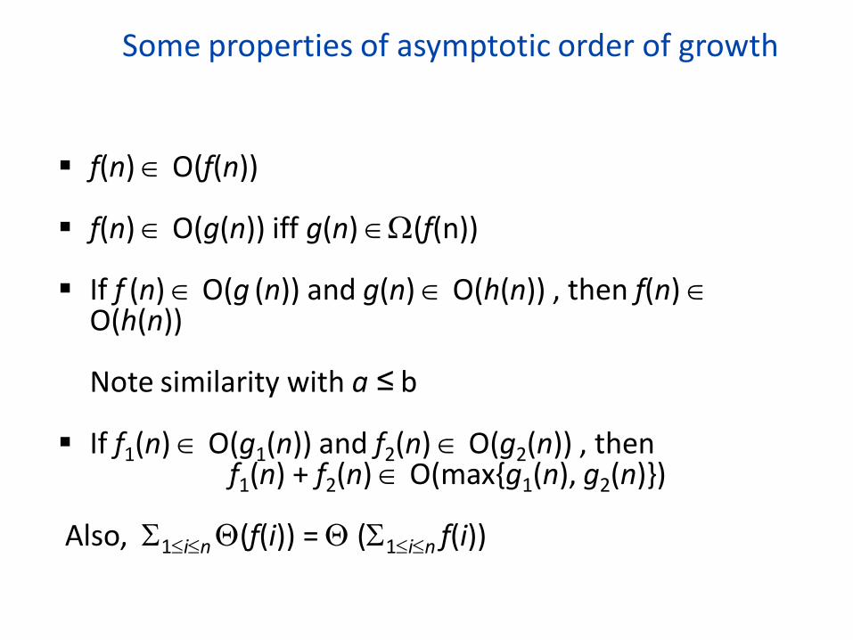
Some properties of asymptotic order of growth
f(n) O(f(n))
f(n) O(g(n)) iff g(n) (f(n))
If f (n) O(g (n)) and g(n) O(h(n)) , then f(n) O(h(n)) Note similarity with a ≤ b
If f1(n) O(g1(n)) and f2(n) O(g2(n)) , then f1(n) + f2(n) O(max{g1(n), g2(n)})
Also, 1in (f(i)) = (1in f(i))

Establishing order of growth using limits
lim T(n)/g(n) =
0 order of growth of T(n) < order of growth of g(n)
c > 0 order of growth of T(n) = order of growth of g(n)
∞ order of growth of T(n) > order of growth of g(n)
n→∞
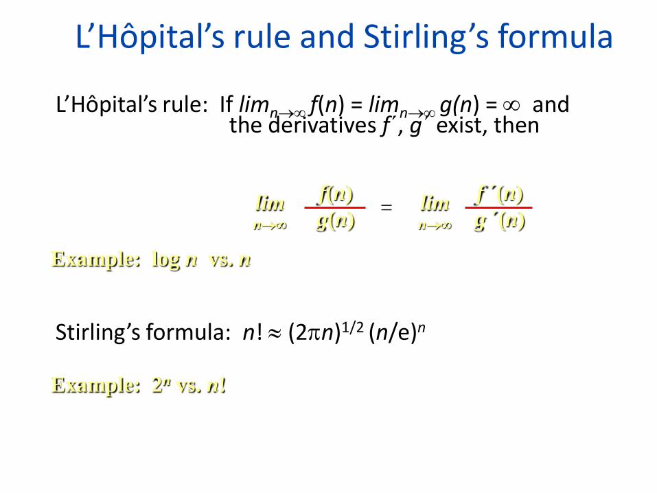
L’Hôpital’s rule and Stirling’s formula
L’Hôpital’s rule: If limn f(n) = limn g(n) = and the derivatives f´, g´ exist, then
Stirling’s formula: n! (2n)1/2 (n/e)n
f(n)
g(n) lim n
= f ´(n)
g ´(n) lim n
Example: log n vs. n
Example: 2n vs. n!

Orders of growth of some important functions
All logarithmic functions loga n belong to the same class (log n) no matter what the logarithm’s base a > 1 is because
All polynomials of the same degree k belong to the same class: akn
k + ak-1nk-1 + … + a0 (nk)
Exponential functions an have different orders of growth for different a’s
order log n < order n (>0) < order an < order n! < order nn
ann bba log/loglog

Basic asymptotic efficiency classes 1 constant
log n logarithmic
n linear
n log n n-log-n
n2 quadratic
n3 cubic
2n exponential
n! factorial

Plan for analyzing nonrecursive algorithms
General Plan for Analysis
Decide on parameter n indicating input size
Identify algorithm’s basiyc operation
Determine worst, average, and best cases for input of size n
Set up a sum for the number of times the basic operation is executed
Simplify the sum using standard formulas and rules (see Appendix A)

Useful summation formulas and rules
lin1 = 1+1+…+1 = n - l + 1 In particular, lin1 = n - 1 + 1 = n (n) 1in i = 1+2+…+n = n(n+1)/2 n2/2 (n2) 1in i
2 = 12+22+…+n2 = n(n+1)(2n+1)/6 n3/3 (n3) 0in a
i = 1 + a +…+ an = (an+1 - 1)/(a - 1) for any a 1 In particular, 0in 2
i = 20 + 21 +…+ 2n = 2n+1 - 1 (2n )
(ai ± bi ) = ai ± bi cai = cai liuai = limai
+ m+1iuai
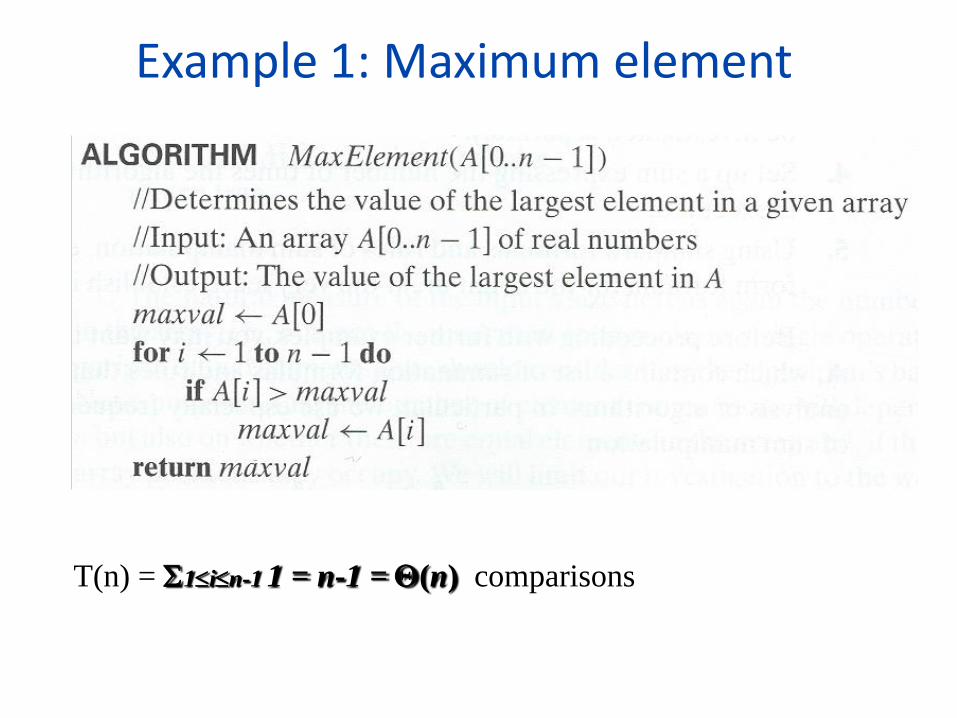
Example 1: Maximum element
T(n) = 1in-1 1 = n-1 = (n) comparisons

Example 2: Element uniqueness problem
T(n) = 0in-2 (i+1jn-1 1)
= 0in-2 n-i-1 = (n-1+1)(n-1)/2
= ( ) comparisons 2n

Example 3: Matrix multiplication
T(n) = 0in-1 0in-1 n
= 0in-1 ( )
= ( ) multiplications
2n
3n

Example 4: Gaussian elimination
Algorithm GaussianElimination(A[0..n-1,0..n]) //Implements Gaussian elimination on an n-by-(n+1) matrix A for i 0 to n - 2 do for j i + 1 to n - 1 do for k i to n do A[j,k] A[j,k] - A[i,k] A[j,i] / A[i,i] Find the efficiency class and a constant factor improvement.
for i 0 to n - 2 do
for j i + 1 to n - 1 do
B A[j,i] / A[i,i]
for k i to n do
A[j,k] A[j,k] – A[i,k] * B

Example 5: Counting binary digits

Plan for Analysis of Recursive Algorithms
Decide on a parameter indicating an input’s size.
Identify the algorithm’s basic operation.
Check whether the number of times the basic op. is executed may vary on different inputs of the same size. (If it may, the worst, average, and best cases must be investigated separately.)
Set up a recurrence relation with an appropriate initial condition expressing the number of times the basic op. is executed.
Solve the recurrence (or, at the very least, establish its solution’s order of growth) by backward substitutions or another method.

Example 1: Recursive evaluation of n!
Definition: n ! = 1 2 … (n-1) n for n ≥ 1 and 0! = 1
Recursive definition of n!: F(n) = F(n-1) n for n ≥ 1 and
F(0) = 1
Size: Basic operation:
n
multiplication
M(n) = M(n-1) + 1
M(0) = 0

Solving the recurrence for M(n)
M(n) = M(n-1) + 1, M(0) = 0 M(n) = M(n-1) + 1
= (M(n-2) + 1) + 1 = M(n-2) + 2
= (M(n-3) + 1) + 2 = M(n-3) + 3
…
= M(n-i) + i
= M(0) + n
= n
The method is called backward substitution.

Solving recurrence for number of moves
M(n) = 2M(n-1) + 1, M(1) = 1 M(n) = 2M(n-1) + 1
= 2(2M(n-2) + 1) + 1 = 2^2*M(n-2) + 2^1 + 2^0
= 2^2*(2M(n-3) + 1) + 2^1 + 2^0
= 2^3*M(n-3) + 2^2 + 2^1 + 2^0
= …
= 2^(n-1)*M(1) + 2^(n-2) + … + 2^1 + 2^0
= 2^(n-1) + 2^(n-2) + … + 2^1 + 2^0
= 2^n - 1

Design and Analysis of Algorithms - Unit II 45
DIVIDE AND CONQUER

Divide and Conquer
Design and Analysis of Algorithms - Unit II 46
The most well known algorithm design strategy:
1. Divide instance of problem into two or more smaller instances
2. Solve smaller instances recursively
3. Obtain solution to original (larger) instance by combining these solutions
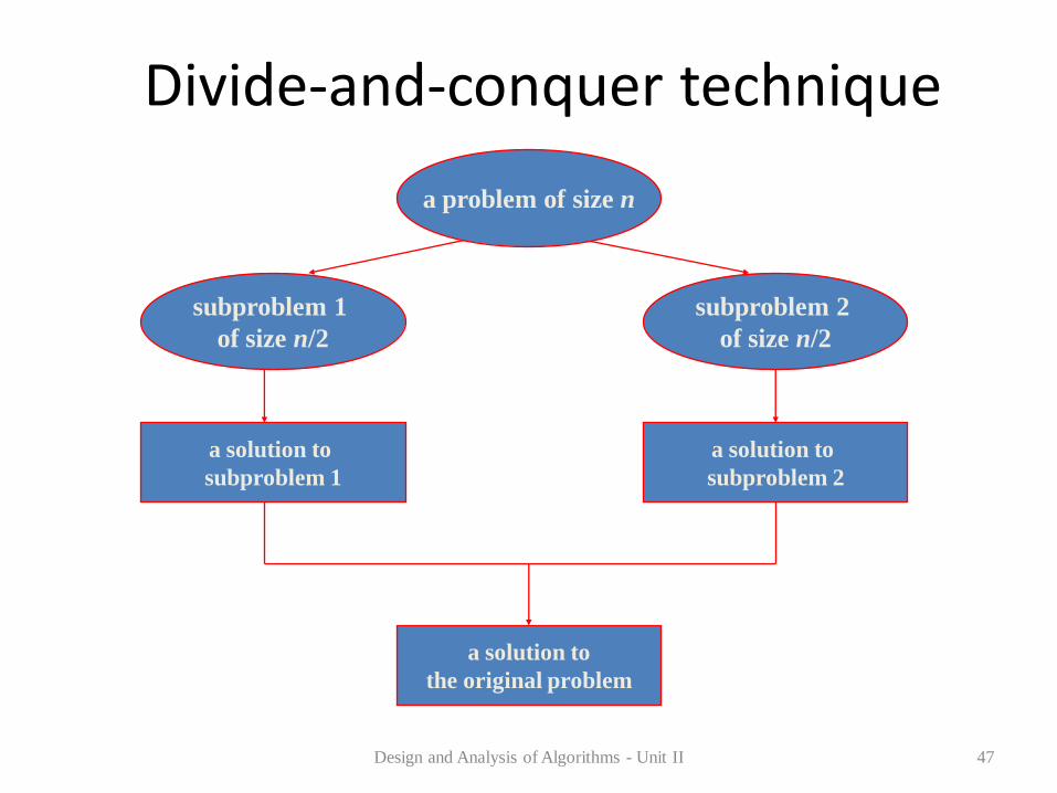
Divide-and-conquer technique
Design and Analysis of Algorithms - Unit II 47
subproblem 2
of size n/2
subproblem 1
of size n/2
a solution to
subproblem 1
a solution to
the original problem
a solution to
subproblem 2
a problem of size n

Divide and Conquer Examples
Design and Analysis of Algorithms - Unit II 48
Sorting: mergesort and quicksort
Tree traversals
Binary search
Matrix multiplication-Strassen’s algorithm
Convex hull-QuickHull algorithm

Design and Analysis of Algorithms - Unit II 49
General Divide and Conquer recurrence:
Master Theorem
T(n) = aT(n/b) + f (n) where f (n) € Θ(nd)
1. a < bd T(n) € Θ(nd)
2. a = bd T(n) € Θ(nd lg n )
3. a > bd T(n) € Θ(nlog b a)
Note: the same results hold with O instead of Θ.

Mergesort
Design and Analysis of Algorithms - Unit II 50
Algorithm: Split array A[1..n] in two and make copies of each half in arrays B[1.. n/2 ] and C[1.. n/2 ] Sort arrays B and C Merge sorted arrays B and C into array A as follows: Repeat the following until no elements remain in one of the
arrays: compare the first elements in the remaining unprocessed portions of
the arrays copy the smaller of the two into A, while incrementing the index
indicating the unprocessed portion of that array
Once all elements in one of the arrays are processed, copy the remaining unprocessed elements from the other array into A.

Mergesort Example
Design and Analysis of Algorithms - Unit II 51
8 3 2 9 7 1 5 4
8 3 2 9 7 1 5 4
8 3 2 9 7 1 5 4
8 3 2 9 7 1 5 4
3 8 2 9 1 7 4 5
2 3 8 9 1 4 5 7
1 2 3 4 5 7 8 9

Pseudocode for Mergesort
Design and Analysis of Algorithms - Unit II 52
ALGORITHM Mergesort(A[0..n-1]) //Sorts array A[0..n-1] by recursive mergesort // Input: An array A[0..n-1] of orderable elements // Output: Array A[0..n-1] sorted in non-increasing
order If n>1 copy A[0..[n/2]-1] to B[0..[n/2]-1] copy A[[n/2]..n-1] to C[0..[n/2]-1] Mergesort(B[0..[n/2]-1]) Mergesort(C[0..[n/2]-1]) Merge(B,C,A)

Pseudocode for Merge
Design and Analysis of Algorithms - Unit II 53
ALGORITHM Merge (B[0..p-1], C[0..q-1], A[0..p+q-1] // Merges two sorted arrays into one sorted array // Input: Arrays B[0..p-1] and C[0..q-1] both sorted // Output: Sorted array A[0..p+q-1] of the elements of B and C i 0; j 0; k0 While i<p and j<q do if B[i]<=C[j] A[k] B[i]; i i+1 else A[k] C[j]; j j+1 k k+1 If i=p copy C[j..q-1] to A[k..p+q-1] Else copy B[i..p-1] to A[k..p+q-1]

Recurrence Relation for Mergesort
Design and Analysis of Algorithms - Unit II 54
• Let T(n) be worst case time on a sequence of n keys
• If n = 1, then T(n) = (1) (constant)
• If n > 1, then T(n) = 2 T(n/2) + (n) – two subproblems of size n/2 each that are solved
recursively
– (n) time to do the merge

Efficiency of mergesort
Design and Analysis of Algorithms - Unit II 55
All cases have same efficiency: Θ( n log n)
Number of comparisons is close to theoretical minimum for comparison-based sorting: log n ! ≈ n lg n - 1.44 n
Space requirement: Θ( n ) (NOT in-place)
Can be implemented without recursion (bottom-
up)

Quick-Sort Quick-sort is a randomized
sorting algorithm based on the divide-and-conquer paradigm:
Divide: pick a random element x (called pivot) and partition S into
L elements less than x
E elements equal x
G elements greater than x
Recur: sort L and G
Conquer: join L, E and G
56 Design and Analysis of
Algorithms - Unit II
x
x
L G E
x
Quicksort
Design and Analysis of Algorithms - Unit II 57
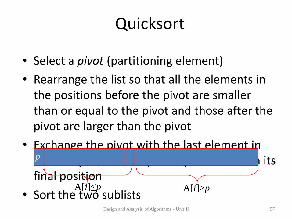
• Select a pivot (partitioning element)
• Rearrange the list so that all the elements in the positions before the pivot are smaller than or equal to the pivot and those after the pivot are larger than the pivot
• Exchange the pivot with the last element in the first (i.e., ≤ sublist) – the pivot is now in its final position
• Sort the two sublists
p
A[i]≤p A[i]>p

The partition algorithm
Design and Analysis of Algorithms - Unit II 58

Efficiency of quicksort
Design and Analysis of Algorithms - Unit II 59
Best case: split in the middle — Θ( n log n) Worst case: sorted array! — Θ( n2) Average case: random arrays — Θ( n log n)
Improvements: better pivot selection: median of three partitioning avoids
worst case in sorted files switch to insertion sort on small subfiles
Considered the method of choice for internal sorting
for large files (n ≥ 10000)

Binary Search - an Iterative Algorithm
Design and Analysis of Algorithms - Unit II 60
Very efficient algorithm for searching in sorted array:
K vs A[0] . . . A[m] . . . A[n-1] If K = A[m], stop (successful search); otherwise, continue searching by the same
method in A[0..m-1] if K < A[m] and in A[m+1..n-1] if K > A[m]

Pseudocode for Binary Search
Design and Analysis of Algorithms - Unit II 61
ALGORITHM BinarySearch(A[0..n-1], K) l 0; r n-1 while l r do // l and r crosses over can’t find K m (l+r)/2 if K = A[m] return m //the key is found else if K < A[m] r m-1 //the key is on the left half of the array else l m+1 // the key is on the right half of
the array return -1

Binary Search – a Recursive Algorithm
Design and Analysis of Algorithms - Unit II 62
ALGORITHM BinarySearchRecur(A[0..n-1], l, r, K) if l > r return –1 else m (l + r) / 2 if K = A[m] return m else if K < A[m] return BinarySearchRecur(A[0..n-1], l, m-1, K) else return BinarySearchRecur(A[0..n-1], m+1, r, K)

Analysis of Binary Search
Worst-case (successful or fail) : Cw (n) = 1 + Cw( n/2 ), Cw (1) = 1
solution: Cw(n) = log2 n +1 = log2(n+1)
This is VERY fast: e.g., Cw(106) = 20 Best-case: successful Cb (n) = 1, fail Cb (n) = log2 n +1
Average-case: successful Cavg(n) = log2 n – 1
fail Cavg(n) = log2(n+1)
Design and Analysis of Algorithms - Unit II 63

Binary Tree Traversals
Design and Analysis of Algorithms - Unit II 64
• Definitions – A binary tree T is defined as a finite set of nodes that is
either empty or consists of a root and two disjoint binary trees TL and TR called, respectively, the left and right subtree of the root.
– The height of a tree is defined as the length of the longest path from the root to a leaf.
• Problem: find the height of a binary tree. T TL R

Pseudocode - Height of a Binary Tree
Design and Analysis of Algorithms - Unit II 65
ALGORITHM Height(T) //Computes recursively the height of a binary
tree //Input: A binary tree T //Output: The height of T if T = return –1 else return max{Height(TL), Height(TR)} + 1

Analysis:
Design and Analysis of Algorithms - Unit II 66
Number of comparisons of a tree T with : 2n + 1
Number of comparisons made to compute
height is the same as number of additions: A(n(T)) = A(n(TL)) + A(n(TR)) +1 for n>0, A(0) = 0 The solution is A(n) = n
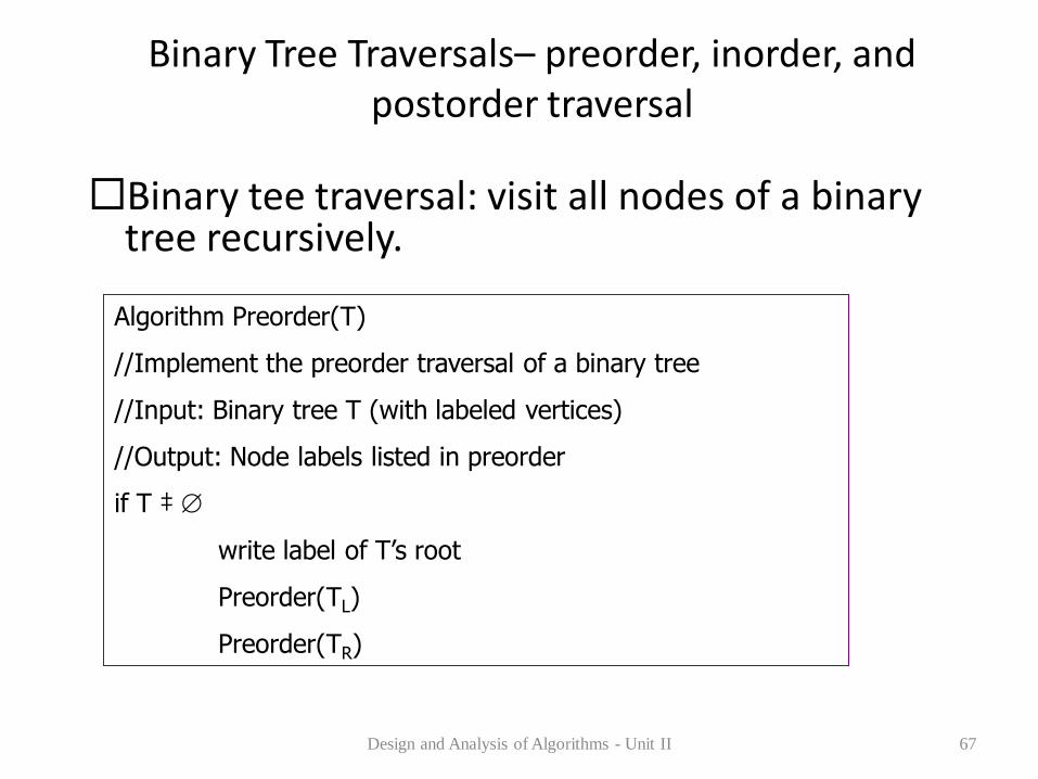
Binary Tree Traversals– preorder, inorder, and postorder traversal
Design and Analysis of Algorithms - Unit II 67
Binary tee traversal: visit all nodes of a binary tree recursively.
Algorithm Preorder(T)
//Implement the preorder traversal of a binary tree
//Input: Binary tree T (with labeled vertices)
//Output: Node labels listed in preorder
if T ‡
write label of T’s root
Preorder(TL)
Preorder(TR)
Multiplication of Large Integers
Design and Analysis of Algorithms - Unit II 68
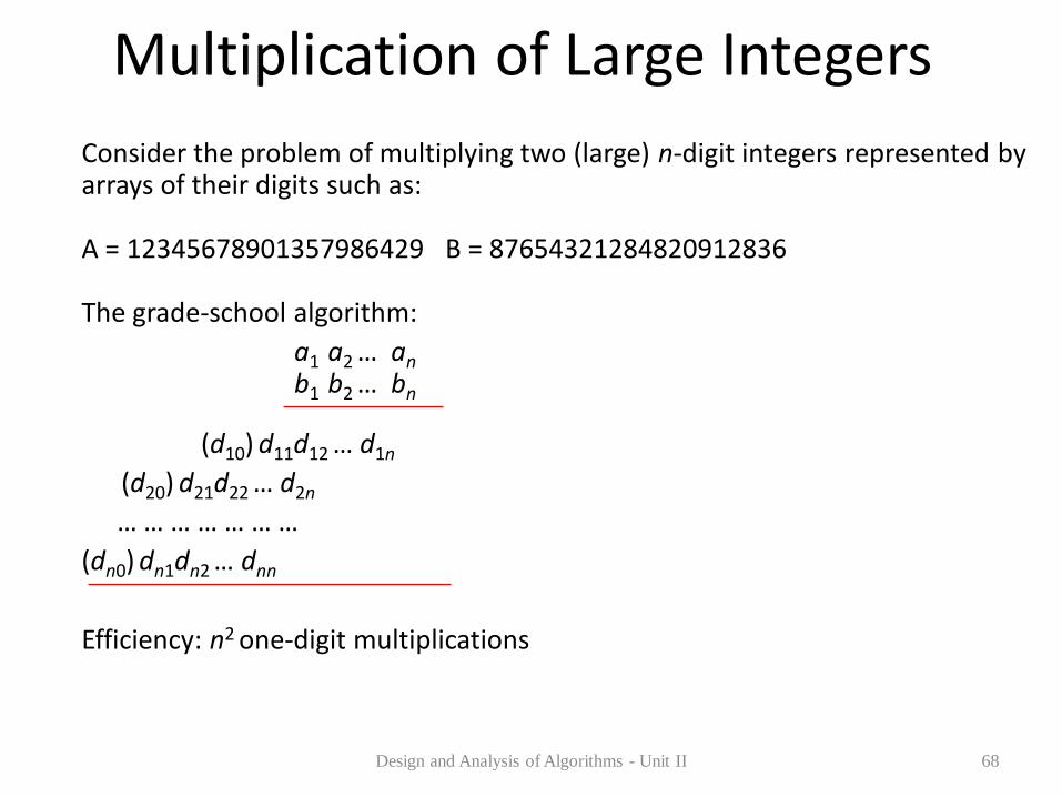
Consider the problem of multiplying two (large) n-digit integers represented by arrays of their digits such as: A = 12345678901357986429 B = 87654321284820912836 The grade-school algorithm:
a1 a2 … an
b1 b2 … bn
(d10) d11d12 … d1n
(d20) d21d22 … d2n
… … … … … … … (dn0) dn1dn2 … dnn
Efficiency: n2 one-digit multiplications

First Divide-and-Conquer Algorithm
Design and Analysis of Algorithms - Unit II 69
A small example: A B where A = 2135 and B = 4014
A = (21·102 + 35), B = (40 ·102 + 14)
So, A B = (21 ·102 + 35) (40 ·102 + 14)
= 21 40 ·104 + (21 14 + 35 40) ·102 + 35 14
In general, if A = A1A2 and B = B1B2 (where A and B are n-digit,
A1, A2, B1, B2 are n/2-digit numbers),
A B = A1 B1·10n + (A1 B2 + A2 B1) ·10n/2 + A2 B2
Recurrence for the number of one-digit multiplications M(n):
M(n) = 4M(n/2), M(1) = 1 Solution: M(n) = n2

Second Divide-and-Conquer Algorithm
Design and Analysis of Algorithms - Unit II 70
A B = A1 B1·10n + (A1 B2 + A2 B1) ·10n/2 + A2 B2
The idea is to decrease the number of multiplications from 4 to 3:
(A1 + A2 ) (B1 + B2 ) = A1 B1 + (A1 B2 + A2 B1) + A2 B2,
I.e., (A1 B2 + A2 B1) = (A1 + A2 ) (B1 + B2 ) - A1 B1 - A2 B2,
which requires only 3 multiplications at the expense of (4-1) extra add/sub.
Recurrence for the number of multiplications M(n): M(n) = 3M(n/2), M(1) = 1
Solution: M(n) = 3log 2n = nlog 23 ≈ n1.585

Strassen’s matrix multiplication
Design and Analysis of Algorithms - Unit II 71
• Strassen observed [1969] that the product of two matrices can be computed as follows:
C00 C01 A00 A01 B00 B01
= *
C10 C11 A10 A11 B10 B11
M1 + M4 - M5 + M7 M3 + M5
=
M2 + M4 M1 + M3 - M2 + M6

Submatrices:
Design and Analysis of Algorithms - Unit II 72
M1 = (A00 + A11) * (B00 + B11)
M2 = (A10 + A11) * B00
M3 = A00 * (B01 - B11)
M4 = A11 * (B10 - B00)
M5 = (A00 + A01) * B11
M6 = (A10 - A00) * (B00 + B01)
M7 = (A01 - A11) * (B10 + B11)

Efficiency of Strassen’s algorithm
Design and Analysis of Algorithms - Unit II 73
• If n is not a power of 2, matrices can be padded with zeros
• Number of multiplications: 7
• Number of additions: 18

Time Analysis
Design and Analysis of Algorithms - Unit II 74

Standard vs Strassen
N Multiplications Additions
Standard alg. 100 1,000,000 990,000
Strassen’s alg. 100 411,822 2,470,334
Standard alg. 1000 1,000,000,000 999,000,000
Strassen’s alg. 1000 264,280,285 1,579,681,709
Standard alg. 10,000 1012 9.99*1011
Strassen’s alg. 10,000 0.169*1012 1012
Design and Analysis of Algorithms - Unit II 75

Greedy Technique

Greedy Technique
77
Constructs a solution to an optimization problem piece by piece through a sequence of choices that are:
• feasible, i.e. satisfying the constraints • locally optimal (with respect to some neighborhood
definition)
• greedy (in terms of some measure), and irrevocable
For some problems, it yields a globally optimal solution for every instance. For most, does not but can be useful for fast
approximations.
Defined by an objective function and a set of constraints

Applications of the Greedy Strategy
78
• Optimal solutions: – change making for “normal” coin denominations
– minimum spanning tree (MST)
– single-source shortest paths
– simple scheduling problems
– Huffman codes
• Approximations/heuristics: – traveling salesman problem (TSP)
– knapsack problem
– other combinatorial optimization problems

Change-Making Problem
79
Given unlimited amounts of coins of denominations d1 > … > dm ,
give change for amount n with the least number of coins Example: d1 = 25c, d2 =10c, d3 = 5c, d4 = 1c and n = 48c Greedy solution: Greedy solution is • optimal for any amount and “normal’’ set of
denominations • may not be optimal for arbitrary coin denominations
<1, 2, 0, 3>
For example, d1 = 25c, d2 = 10c, d3 = 1c, and n = 30c
Q: What are the objective function and constraints?

Minimum Spanning Tree (MST)
80
• Spanning tree of a connected graph G: a connected acyclic subgraph of G that includes all of G’s vertices
• Minimum spanning tree of a weighted, connected graph G: a spanning tree of G of the minimum total weight
Example:
c
d b
a
6
2
4
3
1
c
d b
a
2
3
1
c
d b
a
6
4 1

Prim’s MST algorithm
81
• Start with tree T1 consisting of one (any) vertex and “grow” tree one vertex at a time to produce MST through a series of expanding subtrees T1, T2, …, Tn
• On each iteration, construct Ti+1 from Ti by adding vertex not in Ti that is closest to those already in Ti (this is a “greedy” step!)
• Stop when all vertices are included

Pseudocode – Prim’s algorithm
82
ALGORITHM Prim(G)
// Prim’s algorithm for computing a MST
// Input:A weighted connected graph G = (V,E)
// Output: Et, the set of edges composing a MST of G
VT {v0 }
ET Ø
for I 1 to |v| - 1 do
find a minimum weight edge e*=(v*,u*) among all edges(v,u) such that v is in VT and u is in V – VT
VT VT {u*}
ET ET {v*}
return ET

Example
83
c
d b
a
4
2
6 1
3
c
d b
a
4
2
6 1
3
c
d b
a
4
2
6 1
3
c
d b
a
4
2
6 1
3
c
d b
a
4
2
6 1
3

Notes about Prim’s algorithm
84
• Needs priority queue for locating closest fringe vertex.
• Efficiency – O(n2) for weight matrix representation of graph and array
implementation of priority queue
– O(m log n) for adjacency lists representation of graph with n vertices and m edges and min-heap implementation of the priority queue

Another greedy algorithm for MST: Kruskal’s
85
• Sort the edges in nondecreasing order of lengths
• “Grow” tree one edge at a time to produce MST through a series of expanding forests F1, F2, …, Fn-
1
• On each iteration, add the next edge on the sorted list unless this would create a cycle. (If it would, skip the edge.)

Pseudocode – Kruskal’s algorithm
86
ALGORITHM Kruskal(G)
// Kruskal’s algorithm for constructing a minimum spanning tree
// Input: A weighted connected graph G = (V,E)
// Output: ET, The set of edges composing a MST of G
ET Ø; ecounter 0
k 0
while ecounter < |V| - 1
k k +1
if ET {eik} is acyclic
ET ET {eik} ;
ecounter ecounter + 1
return ET

Example
87
c
d b
a
4
2
6 1
3
c
d b
a
2
6 1
3
c
d b
a
4
2
6 1
3
c
d b
a
4
2
6 1
3
c
d b
a
4
2
6 1
3
c
d b
a
2
1
3

Notes about Kruskal’s algorithm
88
• Algorithm looks easier than Prim’s but is harder to implement (checking for cycles!)
• Cycle checking: a cycle is created iff added edge connects vertices in the same connected component
• Kruskal’s algorithm relies on a union-find algorithm for checking cycles
• Runs in O(m log m) time, with m = |E|. The time is mostly spent on sorting.

Disjoint Sets
89
• Union of two sets A and B, denoted by A B, is the set {x | x A or x B}
• The intersection of two sets A and B, denoted by A ∩ B,
is the set {x| x A and x B}. • Two sets A and B are said to be disjoint if A ∩ B = . • If S = {1,2,…,11} and there are 4 subsets {1,7,10,11} ,
{2,3,5,6}, {4,8} and {9}, these subsets may be labeled as 1, 3, 8 and 9, in this order.

90
Disjoint Sets
• A disjoint-set is a collection ={S1, S2,…, Sk} of distinct dynamic sets.
• Each set is identified by a member of the set, called
representative. • Disjoint-set data structures can be used to solve the
union-find problem Disjoint set operations:
– MAKE-SET(x): create a new set with only x. assume x is not already in some other set.
– UNION(x,y): combine the two sets containing x and y into one new set. A new representative is selected.
– FIND-SET(x): return the representative of the set containing x.

The Union-Find problem
91
• N balls initially, each ball in its own bag
– Label the balls 1, 2, 3, ..., N
• Two kinds of operations:
– Pick two bags, put all balls in these bags into a new bag (Union)
– Given a ball, find the bag containing it (Find)

92
• to design efficient algorithms for Union & Find operations.
• Approach: to represent each set as a rooted tree with data elements stored in its nodes.
• Each element x other than the root has a pointer to its parent p(x) in the tree.
• The root has a null pointer, and it serves as the name or set representative of the set.
• This results in a forest in which each tree corresponds to one set.
• For any element x, let root(x) denote the root of the tree containing x.
– FIND(x) returns root(x).
– union(x, y) means UNION(root(x), root(y)).
OBJECTIVE
Implementation of FIND and UNION
93
• FIND(x) follow the path from x until the root is reached, then return root(x). – Time complexity is O(n) – Find(x) = Find(y), when x and y are in the same set
• UNION(x,y) UNION(FIND(x) , FIND(y) ) UNION(root(x) , root(y) ) UNION(u,v) then let v be the parent of u. Assume u is root(x), v is root(y)
– Time complexity is O(n) – Union(x, y) Combine the set that contains x with the set that contains y

The Union-Find problem
94
• An example with 4 balls
• Initial: {1}, {2}, {3}, {4}
• Union {1}, {3} {1, 3}, {2}, {4}
• Find 3. Answer: {1, 3}
• Union {4}, {1,3} {1, 3, 4}, {2}
• Find 2. Answer: {2}
• Find 1. Answer {1, 3, 4}

Forest Representation
95
• A forest is a collection of trees
• Each bag is represented by a rooted tree, with the root being the representative ball
1
5 3
6
4
2 7
Example: Two bags --- {1, 3, 5} and {2, 4, 6, 7}.

Forest Representation
96
• Find(x)
– Traverse from x up to the root
• Union(x, y)
– Merge the two trees containing x and y
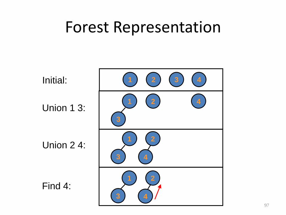
Forest Representation
97
Initial:
Union 1 3:
Union 2 4:
Find 4:
1 3 4 2
1
3
4 2
1
3 4
2
1
3 4
2

Forest Representation
98
Union 1 4:
Find 4:
1
3
4
2
1
3
4
2

99
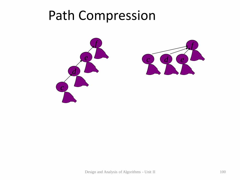
Union by Rank & Path Compression
• Union by Rank: Each node is associated with a rank, which is the upper bound on the height of the node (i.e., the height of subtree rooted at the node), then when UNION, let the root with smaller rank point to the root with larger rank.
• Path Compression: used in FIND-SET(x) operation, make each node in the path from x to the root directly point to the root. Thus reduce the tree height.
Design and Analysis of Algorithms - Unit II 100
Path Compression
f
e
d
c
f
e d c

Shortest paths – Dijkstra’s algorithm
Design and Analysis of Algorithms - Unit II 101
Single Source Shortest Paths Problem: Given a weighted
connected (directed) graph G, find shortest paths from source vertex s
to each of the other vertices
Dijkstra’s algorithm: Similar to Prim’s MST algorithm, with
a different way of computing numerical labels: Among vertices
not already in the tree, it finds vertex u with the smallest sum
dv + w(v,u)
where
v is a vertex for which shortest path has been already found on preceding iterations (such vertices form a tree rooted at s)
dv is the length of the shortest path from source s to v w(v,u) is the length (weight) of edge from v to u

Pseudocode – Dijkstra’s algorithm
Design and Analysis of Algorithms - Unit II 102
ALGORITHM Dijkstra(G,S) // Dijkstra’s algorithm for single source shortest paths // Input: A weighted connected graph G= (V,E) and its vertex s // Output: The length dv of a shortest path from s to v and its penultimate vertex pv for every vertex v in V Initialize(Q) for every vertex v in V do dv∞;pv=null Insert(Q,v,dv) ds0; Decrease(Q, s, ds) VT Ø for I 1 to |v| - 1 do u* DeleteMin(Q) VT VT {u*} for every vertex u in V - VT that is adjacent to u* do if du + w(u*, u) < du du du * + w(u*,u); pu u* Decrease (Q,u, du )

Example
Design and Analysis of Algorithms - Unit II 103
d 4
Tree vertices Remaining vertices
a(-,0) b(a,3) c(-,∞) d(a,7) e(-,∞)
a
b 4
e
3
7
6 2 5
c
a
b
d
4 c
e
3
7 4
6 2 5
a
b
d
4 c
e
3
7 4
6 2 5
a
b
d
4 c
e
3
7 4
6 2 5
b(a,3) c(b,3+4) d(b,3+2) e(-,∞)
d(b,5) c(b,7) e(d,5+4)
c(b,7) e(d,9)
e(d,9)
d
a
b
d
4 c
e
3
7 4
6 2 5

Notes on Dijkstra’s algorithm
104
• Doesn’t work for graphs with negative weights (whereas Floyd’s algorithm does, as long as there is no negative cycle).
• Applicable to both undirected and directed
graphs
• Efficiency – O(|V|2) for graphs represented by weight matrix and array
implementation of priority queue – O(|E|log|V|) for graphs represented by adj. lists and min-
heap implementation of priority queue

Graphs
Minimum Spanning Tree
PLSD210

Key Points • Dynamic Algorithms
• Optimal Binary Search Tree
– Used when
• some items are requested more often than others
• frequency for each item is known
– Minimises cost of all searches
– Build the search tree by
• Considering all trees of size 2, then 3, 4, ....
• Larger tree costs computed from smaller tree costs
– Sub-trees of optimal trees are optimal trees!
• Construct optimal search tree by saving root of each optimal sub-tree and tracing back
• O(n3) time / O(n2) space

Key Points • Other Problems using Dynamic Algorithms
• Matrix chain multiplication
– Find optimal parenthesisation of a matrix product
• Expressions within parentheses
– optimal parenthesisations themselves
• Optimal sub-structure characteristic of dynamic algorithms
• Similar to optimal binary search tree
• Longest common subsequence
– Longest string of symbols found in each of two sequences
• Optimal triangulation
– Least cost division of a polygon into triangles
– Maps to matrix chain multiplication

Graphs - Definitions • Graph
– Set of vertices (nodes) and edges connecting them
– Write
G = ( V, E ) where
• V is a set of vertices: V = { vi }
• An edge connects two vertices: e = ( vi , vj )
• E is a set of edges: E = { (vi , vj ) }
Vertices
Edges

Graphs - Definitions • Path
– A path, p, of length, k, is a sequence of connected vertices
– p = <v0,v1,...,vk> where (vi,vi+1) E < i, c, f, g, h > Path of length 5
< a, b >
Path of length 2

Graphs - Definitions • Cycle
– A graph contains no cycles if there is no path
– p = <v0,v1,...,vk> such that v0 = vk
< i, c, f, g, i > is a cycle

Graphs - Definitions • Spanning Tree
– A spanning tree is a set of |V|-1 edges that connect all the vertices of a graph
The red path connects
all vertices,
so it’s a spanning tree

Graphs - Definitions • Minimum Spanning Tree
– Generally there is more than one spanning tree
– If a cost cij is associated with edge eij = (vi,vj)
then the minimum spanning tree is the set of edges Espan such that
C = ( cij | " eij Espan ) is a minimum
The red tree is the
Min ST
Other ST’s can be formed ..
• Replace 2 with 7
• Replace 4 with 11
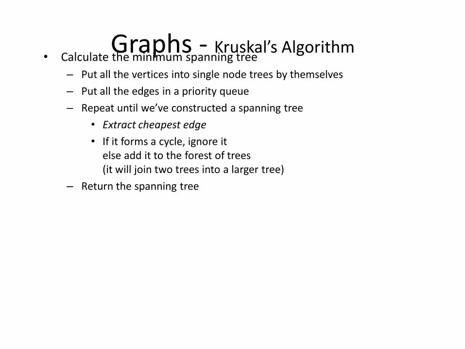
Graphs - Kruskal’s Algorithm • Calculate the minimum spanning tree
– Put all the vertices into single node trees by themselves
– Put all the edges in a priority queue
– Repeat until we’ve constructed a spanning tree
• Extract cheapest edge
• If it forms a cycle, ignore it else add it to the forest of trees (it will join two trees into a larger tree)
– Return the spanning tree
• Note that this algorithm makes no attempt
• to be clever
• to make any sophisticated choice of the next edge
• it just tries the cheapest one!

Graphs - Kruskal’s Algorithm in C Forest MinimumSpanningTree( Graph g, int n,
double **costs ) {
Forest T;
Queue q;
Edge e;
T = ConsForest( g );
q = ConsEdgeQueue( g, costs );
for(i=0;i<(n-1);i++) {
do {
e = ExtractCheapestEdge( q );
} while ( !Cycle( e, T ) );
AddEdge( T, e );
}
return T;
}
Initial Forest: single vertex trees
P Queue of edges

Graphs - Kruskal’s Algorithm in C Forest MinimumSpanningTree( Graph g, int n,
double **costs ) {
Forest T;
Queue q;
Edge e;
T = ConsForest( g );
q = ConsEdgeQueue( g, costs );
for(i=0;i<(n-1);i++) {
do {
e = ExtractCheapestEdge( q );
} while ( !Cycle( e, T ) );
AddEdge( T, e );
}
return T;
}
We need n-1 edges
to fully connect (span)
n vertices

Graphs - Kruskal’s Algorithm in C Forest MinimumSpanningTree( Graph g, int n,
double **costs ) {
Forest T;
Queue q;
Edge e;
T = ConsForest( g );
q = ConsEdgeQueue( g, costs );
for(i=0;i<(n-1);i++) {
do {
e = ExtractCheapestEdge( q );
} while ( !Cycle( e, T ) );
AddEdge( T, e );
}
return T;
}
Try the cheapest edge
Until we find one that doesn’t
form a cycle
... and add it to the forest
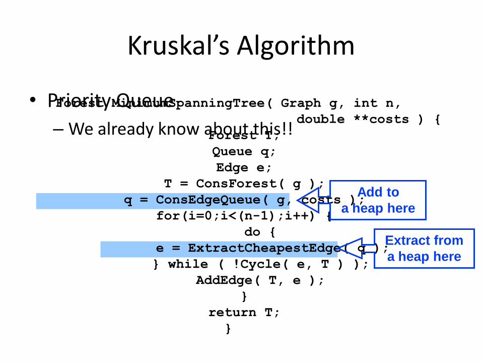
Kruskal’s Algorithm
• Priority Queue
– We already know about this!!
Forest MinimumSpanningTree( Graph g, int n,
double **costs ) {
Forest T;
Queue q;
Edge e;
T = ConsForest( g );
q = ConsEdgeQueue( g, costs );
for(i=0;i<(n-1);i++) {
do {
e = ExtractCheapestEdge( q );
} while ( !Cycle( e, T ) );
AddEdge( T, e );
}
return T;
}
Add to
a heap here
Extract from
a heap here

Kruskal’s Algorithm
• Cycle detection
Forest MinimumSpanningTree( Graph g, int n,
double **costs ) {
Forest T;
Queue q;
Edge e;
T = ConsForest( g );
q = ConsEdgeQueue( g, costs );
for(i=0;i<(n-1);i++) {
do {
e = ExtractCheapestEdge( q );
} while ( !Cycle( e, T ) );
AddEdge( T, e );
}
return T;
}
But how do
we detect a
cycle?

Kruskal’s Algorithm • Cycle detection
– Uses a Union-find structure
– For which we need to understand a partition of a set
• Partition
– A set of sets of elements of a set
• Every element belongs to one of the sub-sets
• No element belongs to more than one sub-set
– Formally:
• Set, S = { si }
• Partition(S) = { Pi }, where Pi = { si }
" si S, si Pj
• " j, k P P =
Pi are subsets of S
All si belong to one of the Pj
None of the Pi
have common elements
S is the union of all the Pi

Kruskal’s Algorithm • Partition
– The elements of each set of a partition
• are related by an equivalence relation
• equivalence relations are – reflexive
– transitive
– symmetric
– The sets of a partition are equivalence classes
• Each element of the set is related to every other element
x ~ x
if x ~ y and y ~ z, then x ~ z
if x ~ y, then y ~ x

Kruskal’s Algorithm • Partitions
– In the MST algorithm, the connected vertices form equivalence classes
• “Being connected” is the equivalence relation
– Initially, each vertex is in a class by itself
– As edges are added, more vertices become related and the equivalence classes grow
– Until finally all the vertices are in a single equivalence class

Kruskal’s Algorithm • Representatives
– One vertex in each class may be chosen as the representative of that class
– We arrange the vertices in lists that lead to the representative
• This is the union-find structure
• Cycle determination

Kruskal’s Algorithm • Cycle determination
– If two vertices have the same representative, they’re already connected and adding a further connection between them is pointless
– Procedure:
• For each end-point of the edge that you’re going to add
• follow the lists and find its representative
• if the two representatives are equal, then the edge will form a cycle

Kruskal’s Algorithm in operation
Each vertex is its
own representative
All the vertices are in
single element trees

Kruskal’s Algorithm in operation
The cheapest edge
is h-g
All the vertices are in
single element trees
Add it to the forest,
joining h and g into a
2-element tree

Kruskal’s Algorithm in operation
The cheapest edge
is h-g
Add it to the forest,
joining h and g into a
2-element tree
Choose g as its
representative

Kruskal’s Algorithm in operation The next cheapest edge
is c-i Add it to the forest,
joining c and i into a
2-element tree
Choose c as its
representative
Our forest now has 2 two-element trees
and 5 single vertex ones

Kruskal’s Algorithm in operation The next cheapest edge
is a-b Add it to the forest,
joining a and b into a
2-element tree
Choose b as its
representative
Our forest now has 3 two-element trees
and 4 single vertex ones

Kruskal’s Algorithm in operation The next cheapest edge
is c-f Add it to the forest,
merging two
2-element trees
Choose the rep of one
as its representative

Kruskal’s Algorithm in operation
The next cheapest edge
is g-i
The rep of g is c
\ g-i forms a cycle
The rep of i is also c
It’s clearly not needed!

Kruskal’s Algorithm in operation
The next cheapest edge
is c-d
The rep of c is c
\ c-d joins two
trees, so we add it
The rep of d is d
.. and keep c as the representative

Kruskal’s Algorithm in operation The next cheapest edge
is h-i
The rep of h is c
\ h-i forms a cycle,
so we skip it
The rep of i is c

Kruskal’s Algorithm in operation The next cheapest edge
is a-h
The rep of a is b
\ a-h joins two trees,
and we add it
The rep of h is c

Kruskal’s Algorithm in operation The next cheapest edge
is b-c But b-c forms a cycle
... and we now have a spanning tree
So add d-e instead
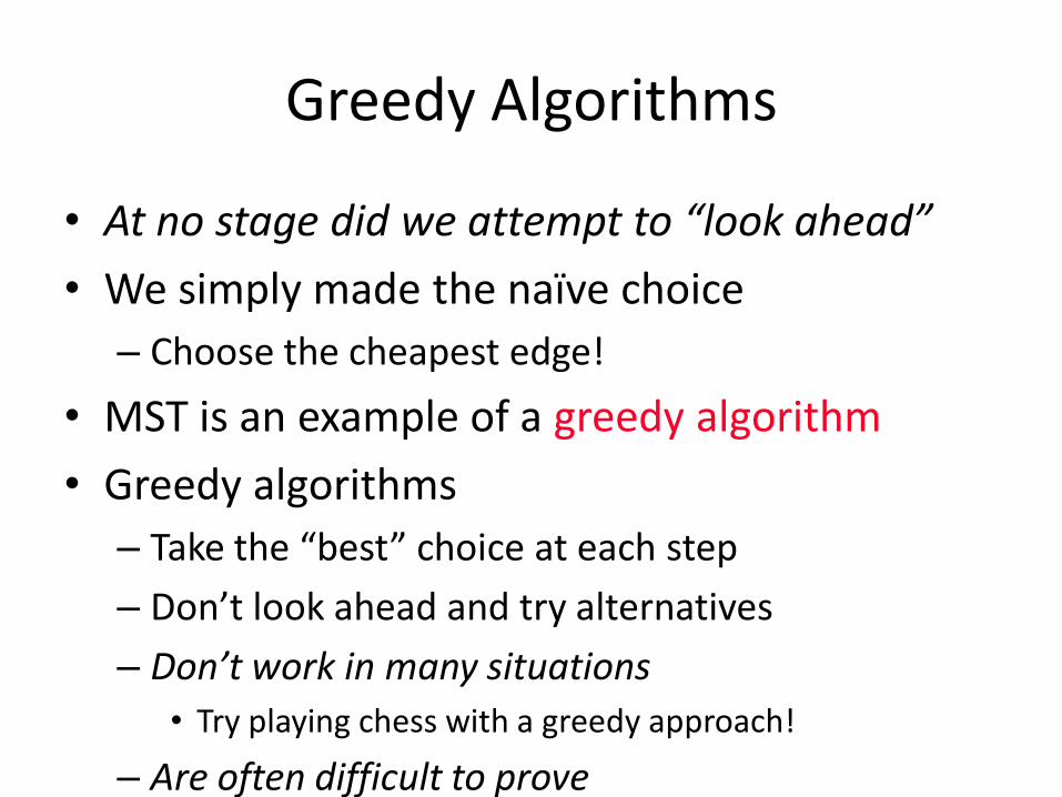
Greedy Algorithms
• At no stage did we attempt to “look ahead”
• We simply made the naïve choice
– Choose the cheapest edge!
• MST is an example of a greedy algorithm
• Greedy algorithms
– Take the “best” choice at each step
– Don’t look ahead and try alternatives
– Don’t work in many situations
• Try playing chess with a greedy approach!
– Are often difficult to prove

Proving Greedy Algorithms
• MST Proof
– “Proof by contradiction” is usually the best approach!
– Note that
• any edge creating a cycle is not needed
\Each edge must join two sub-trees
– Suppose that the next cheapest edge, ex, would join trees Ta and Tb
– Suppose that instead of ex we choose ez - a more expensive edge, which joins Ta and Tc
– But we still need to join Tb to Ta or some other tree to which T is connected

MST - Time complexity
• Steps
– Initialise forest O( |V| )
– Sort edges O( |E|log|E| )
• Check edge for cycles O( |V| ) x
• Number of edges O( |V| ) O( |V|2 )
– Total O(
|V|+|E|log|E|+|V|2 )
– Since |E| = O( |V|2 ) O( |V|2 log|V| )
– Thus we would class MST as O( n2 log n )
for a graph with n vertices
This is an upper bound,
Here’s the
“professionals read textbooks”
theme recurring again!

UNIT-IV
BACKTRACKING

Tackling Difficult Combinatorial Problems
There are two principal approaches to tackling difficult combinatorial problems (NP-hard problems):
Use a strategy that guarantees solving the problem exactly but doesn’t guarantee to find a solution in polynomial time
Use an approximation algorithm that can find an approximate (sub-optimal) solution in polynomial time

Exact Solution Strategies • exhaustive search (brute force)
– useful only for small instances
• dynamic programming
– applicable to some problems (e.g., the knapsack problem)
• backtracking
– eliminates some unnecessary cases from consideration
– yields solutions in reasonable time for many instances but worst case is still exponential
• branch-and-bound
– further refines the backtracking idea for optimization problems

Backtracking
Construct the state-space tree nodes: partial solutions edges: choices in extending partial solutions
Explore the state space tree using depth-first search
“Prune” nonpromising nodes dfs stops exploring subtrees rooted at nodes that cannot lead to
a solution and backtracks to such a node’s parent to continue the search

Example: n-Queens Problem
Place n queens on an n-by-n chess board so that no two of them are in the same row, column, or diagonal
1 2 3 4
1
2
3
4
queen 1
queen 2
queen 3
queen 4

State-Space Tree of the 4-Queens Problem

n-Queens Problem
Algorithm NQueens(k,n) { for i=1 to n do { if place(k,i) then { x[k]=i; if (k = n) then write (x[1:n]); else NQueens(k+1, n); } } NQueens(k-1,n); i= x[k-1]+1; }

n-Queens Problem
Algorithm place(k,i)
// To place a new queen in the chessboard
// Returns true if a queen can be placed in kth row and ith column, otherwise false.
// x[ ] is a global array whose first (k-1) values have been set
// Abs(r) returns the absolute value of r
{
for j = 1 to k-1 do
if ((x[j] = i) or (Abs (j-k))) then
return false;
return true;
}

Hamiltonian Circuit
Hamiltonian Path: is a path in an undirected graph which visits each vertex exactly once
Hamiltonian circuit: is a cycle in an undirected graph which visits each vertex exactly once and also returns to the starting vertex.
Determining whether such paths and cycles
exists is the hamiltonian path problem.
Hamiltonian paths and cycles are named after William Rowan Hamilton

State Space Tree of Hamiltonian Circuit Problem
d
a b
e
c f0
1
2
3 6
9
10
11
12
8 7 4
5
Dead-end
Dead-end
Sol.
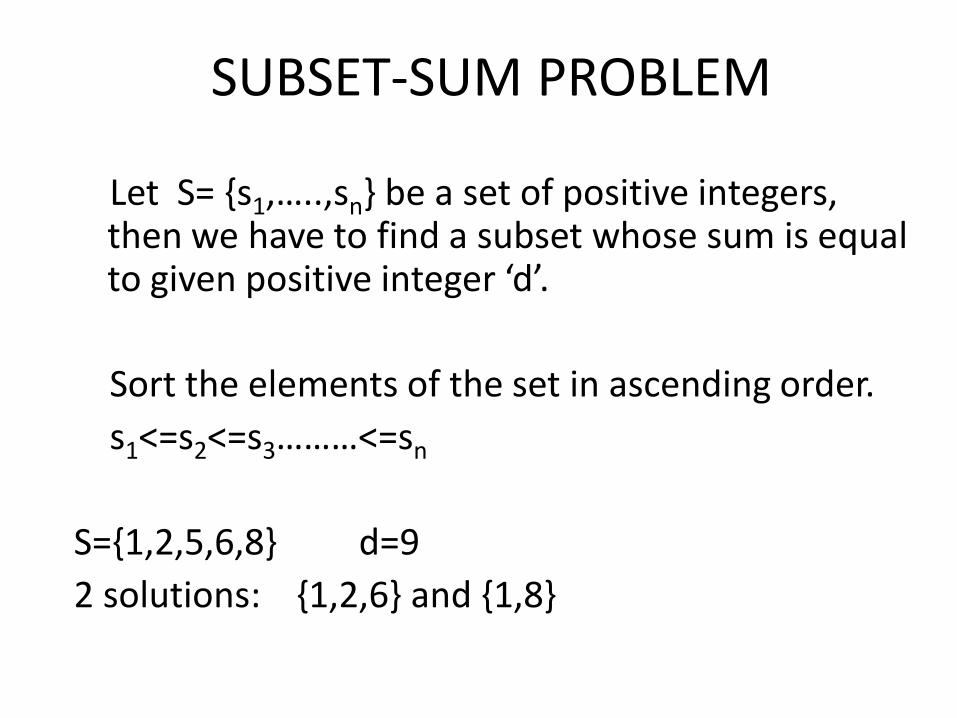
SUBSET-SUM PROBLEM
Let S= {s1,…..,sn} be a set of positive integers, then we have to find a subset whose sum is equal to given positive integer ‘d’.
Sort the elements of the set in ascending order.
s1<=s2<=s3………<=sn
S={1,2,5,6,8} d=9
2 solutions: {1,2,6} and {1,8}

Subset – Sum Problem
Steps:
1. The root of the tree represents the starting point, with no decisions about the given elements.
2. Its left and right children represent, inclusion and exclusion of s1 in the set being sought
3. Going to the left from a node of the first level corresponds to inclusion of s2, while going to right corresponds to exclusion
4. A path from the root to a node at the ith level of the tree indicates which of the first i numbers have been included in the subsets represented by that nodeWe record the value of s’, the sum of these numbers in the node.
5. If s’ =d, we have a solution to the problem and stop. If all the solutions need to be found, continue by backtracking to the node’s parent.
6. If s’ is not equal to d, we can terminate the node as nonpromising if either of the two equalities holds.
7. s’+si+1 > d ( the sum s’ too large) n s’ + ∑ sj < d ( the sum s’ too small) j=i+1

State Space Tree of Subset – Sum Problem
0
0
05
11 5
3
38
3
with 3
with 5
with 6
w/o 3
w/o 5
w/o 6 with 6 w/o 6
w/o 5 with 5
X X X X
X
14+7>15 3+7<15 11+7>14 5+7<15
0+13<15with 6
X
9+7>15
14 98
8
w/o 7
w/o 6
X8<15
solution
with 7
15
S= {3,5,6,7} and d=15
No. of Nodes in the state space tree is 1+2+22+…+2n = 2n+1 -1

Pseudocode: Backtracking

BRANCH AND BOUND

• Branch and bound (BB) is a general algorithm for finding optimal solutions of various optimization problems, especially in discrete and combinatorial optimization.
• It consists of a systematic enumeration of all candidate solutions, where large subsets of fruitless candidates are discarded, by using upper and lower estimated bounds of the quantity being optimized.
Branch-and-Bound

156
Branch-and-Bound
• In the standard terminology of optimization problems, a feasible solution is a point in the problem’s search space that satisfies all the problem’s constraints
• An optimal solution is a feasible solution with the best value of the objective function

157
Branch-and-Bound
• 3 Reasons for terminating a search path at the current node in a state-space tree of a branch-and-bound algorithm:
1. The value of the node’s bound is not better than the value of the best solution seen so far.
2. The node represents no feasible solutions because the constraints of the problem are already violated.
3. The subset of feasible solutions represented by the node consists of a single point—in this case we compare the value of the objective function for this feasible solution with that of the best solution seen so far and update the latter with the former if the new solution is better.

Branch-and-Bound
• An enhancement of backtracking
• Applicable to optimization problems
• For each node (partial solution) of a state-space tree, computes a bound on the value of the objective function for all descendants of the node (extensions of the partial solution)
• Uses the bound for: – ruling out certain nodes as “nonpromising” to prune the tree – if a node’s bound is
not better than the best solution seen so far – guiding the search through state-space

Select one element in each row of the cost matrix C so that: • no two selected elements are in the same column • the sum is minimized Example
Job 1 Job 2 Job 3 Job 4
Person a 9 2 7 8
Person b 6 4 3 7
Person c 5 8 1 8
Person d 7 6 9 4
Lower bound: Any solution to this problem will have total cost
at least: 2 + 3 + 1 + 4 (or 5 + 2 + 1 + 4)
Example: Assignment Problem

Example: First two levels of the state-space tree

Example (cont.)

Example: Complete state-space tree

Solution:
• Person a – job 2
• Person b – job 1
• Person c – job 3
• Person d – job 4

KNAPSACK PROBLEM
• N items of known weights wi and values vi, i=1,2,….n
• Knapsack capacity W =10
• Item Weight Value Value/Weight
1 4 $40 10
2 7 $42 6
3 5 $25 5
4 3 $12 4
ub = v+ (W-w) (v /w )

State space tree of knapsack problem
ub=100
w=0, v=0
ub=76
w=4, v=40
ub=60
w=0, v=0
w=11
ub=70
w=4, v=40
ub=69
w=9, v=65
ub=64
w=4, v=40
w=12
ub=65
w=9, v=65
0
1
3
2
4
5 6
7 8
with 1 w/o 1
with 2 w/o 2
with 3 w/o 3
with 4 w/o 4
X
X
X
X
not feasible
not feasible
inferior to node 8
inferior to node 8
Optimal Solution

Traveling Salesman Problem
• For each city i, 1 <= i <=n, find the sum of the distances from city i to the two nearest cities.
• Compute the sum s of these n numbers
• Divide the result by 2
• If all the distances are integers, round up the result to the nearest integer
• lb = [ s/2 ]

Example: Traveling Salesman Problem

UNIT - V
NP PROBLEMS & APPROXIMATION
ALGORITHMS

P, NP and NP-Complete Problems

Problem Types: Optimization and Decision
Optimization problem: find a solution that maximizes or minimizes some objective function
Decision problem: answer yes/no to a question
Many problems have decision and optimization versions. E.g.: traveling salesman problem optimization: find Hamiltonian cycle of minimum length decision: find Hamiltonian cycle of length m
Decision problems are more convenient for formal
investigation of their complexity.

Class P P: the class of decision problems that are solvable in
O(p(n)) time, where p(n) is a polynomial of problem’s input size n
Examples: searching
element uniqueness
graph connectivity
graph acyclicity
primality testing

Class NP NP (nondeterministic polynomial): class of decision
problems whose proposed solutions can be verified in polynomial time = solvable by a nondeterministic polynomial algorithm
A nondeterministic polynomial algorithm is an abstract two-stage procedure that:
generates a random string purported to solve the problem
checks whether this solution is correct in polynomial time
By definition, it solves the problem if it’s capable of generating and verifying a solution on one of its tries

Example: CNF satisfiability Problem: Is a boolean expression in its conjunctive
normal form (CNF) satisfiable, i.e., are there values of its variables that makes it true?
This problem is in NP. Nondeterministic algorithm: Guess truth assignment Substitute the values into the CNF formula to
see if it evaluates to true
Example: (A | ¬B | ¬C) & (A | B) & (¬B | ¬D | E) & (¬D | ¬E) Truth assignments:
A B C D E 0 0 0 0 0
. . . 1 1 1 1 1
Checking phase: O(n)

What problems are in NP?
• Hamiltonian circuit existence
• Partition problem: Is it possible to partition a set of n integers into two disjoint subsets with the same sum?
• Decision versions of TSP, knapsack problem, graph coloring, and many other combinatorial optimization problems. (Few exceptions include: MST, shortest paths)
• All the problems in P can also be solved in this manner (but no guessing is necessary), so we have:

NP-Complete Problems A decision problem D is NP-complete if it’s as hard as any
problem in NP, i.e.,
• D is in NP
• every problem in NP is polynomial-time reducible to D
Cook’s theorem (1971): CNF-sat is NP-complete
NP-complete
problem
NP problems

NP-Complete Problems (cont.)
Other NP-complete problems obtained through polynomial-
time reductions from a known NP-complete problem
known
NP-complete
problem
NP problems
candidate
for NP -
completeness

P = NP ? Dilemma Revisited • P = NP would imply that every problem in NP, including all NP-
complete problems, could be solved in polynomial time
• If a polynomial-time algorithm for just one NP-complete problem is discovered, then every problem in NP can be solved in polynomial time, i.e., P = NP
• Most but not all researchers believe that P NP , i.e. P is a proper subset of NP
NP-complete
problem
NP problems


![Development of a fuzzy logic-based loading algorithm in ... · qian Shao, and Zhihong Jin.(2015) [13] present a two-phase hybrid dynamic algorithm aiming at obtaining an optimized](https://img.pdfslide.net/doc/110x75/6039ff4520400d66e5758fe2/development-of-a-fuzzy-logic-based-loading-algorithm-in-qian-shao-and-zhihong.jpg)