CHAPTER 2 HYDROLOGY 22 February 2000 - lincoln.ne.gov · Hydrology Drainage Criteria Manual 2 - 1 2.1 Overview 2.1.1 Introduction Estimation of the peak rate of runoff, volume of

CHAPTER 2

HYDROLOGY

22 February 2000

Drainage Criteria Manual

Chapter Two - Hydrology

Table Of Contents2.1 Overview . . . . . . . . . . . . . . . . . . . . . . . . . . . . . . . . . . . . . . . . . . . . . . . . . . . . . . . . . . . . . . . . . . . . . . . . . . . . . . . 2 - 1

2.1.1 Introduction . . . . . . . . . . . . . . . . . . . . . . . . . . . . . . . . . . . . . . . . . . . . . . . . . . . . . . . . . . . . . . . . . . . . . . . 2 - 12.1.2 Factors Affecting Floods . . . . . . . . . . . . . . . . . . . . . . . . . . . . . . . . . . . . . . . . . . . . . . . . . . . . . . . . . . . . . . 2 - 12.1.3 Hydrologic Method Selection . . . . . . . . . . . . . . . . . . . . . . . . . . . . . . . . . . . . . . . . . . . . . . . . . . . . . . . . . . 2 - 2

2.2 Symbols And Definitions . . . . . . . . . . . . . . . . . . . . . . . . . . . . . . . . . . . . . . . . . . . . . . . . . . . . . . . . . . . . . . . . . . . 2 - 32.3 Concept Definitions . . . . . . . . . . . . . . . . . . . . . . . . . . . . . . . . . . . . . . . . . . . . . . . . . . . . . . . . . . . . . . . . . . . . . . . 2 - 32.4 Design Frequency . . . . . . . . . . . . . . . . . . . . . . . . . . . . . . . . . . . . . . . . . . . . . . . . . . . . . . . . . . . . . . . . . . . . . . . . 2 - 5

2.4.1 Overview . . . . . . . . . . . . . . . . . . . . . . . . . . . . . . . . . . . . . . . . . . . . . . . . . . . . . . . . . . . . . . . . . . . . . . . . . 2 - 52.4.2 Frequency Design Criteria . . . . . . . . . . . . . . . . . . . . . . . . . . . . . . . . . . . . . . . . . . . . . . . . . . . . . . . . . . . . . 2 - 5

2.5 Rational Method . . . . . . . . . . . . . . . . . . . . . . . . . . . . . . . . . . . . . . . . . . . . . . . . . . . . . . . . . . . . . . . . . . . . . . . . . 2 - 62.5.1 Introduction . . . . . . . . . . . . . . . . . . . . . . . . . . . . . . . . . . . . . . . . . . . . . . . . . . . . . . . . . . . . . . . . . . . . . . . 2 - 62.5.2 Concept and Equation . . . . . . . . . . . . . . . . . . . . . . . . . . . . . . . . . . . . . . . . . . . . . . . . . . . . . . . . . . . . . . . . 2 - 62.5.3 Application . . . . . . . . . . . . . . . . . . . . . . . . . . . . . . . . . . . . . . . . . . . . . . . . . . . . . . . . . . . . . . . . . . . . . . . . 2 - 6

2.5.3.1 Time Of Concentration . . . . . . . . . . . . . . . . . . . . . . . . . . . . . . . . . . . . . . . . . . . . . . . . . . . . . . . . . 2 - 62.5.3.1.1 Common Errors . . . . . . . . . . . . . . . . . . . . . . . . . . . . . . . . . . . . . . . . . . . . . . . . . . . . . . . . . . . . 2 - 9

2.5.3.2 Rainfall Intensity . . . . . . . . . . . . . . . . . . . . . . . . . . . . . . . . . . . . . . . . . . . . . . . . . . . . . . . . . . . . . . 2 - 92.5.3.3 Runoff Coefficient . . . . . . . . . . . . . . . . . . . . . . . . . . . . . . . . . . . . . . . . . . . . . . . . . . . . . . . . . . . . 2 - 11

2.5.3.3.1 Infrequent Storm . . . . . . . . . . . . . . . . . . . . . . . . . . . . . . . . . . . . . . . . . . . . . . . . . . . . . . . . . . 2 - 122.5.4 Limitations . . . . . . . . . . . . . . . . . . . . . . . . . . . . . . . . . . . . . . . . . . . . . . . . . . . . . . . . . . . . . . . . . . . . . . . 2 - 122.5.5 Example Problem - Rational Method . . . . . . . . . . . . . . . . . . . . . . . . . . . . . . . . . . . . . . . . . . . . . . . . . . . . . 2 - 13

2.6 SCS Unit Hydrograph Method . . . . . . . . . . . . . . . . . . . . . . . . . . . . . . . . . . . . . . . . . . . . . . . . . . . . . . . . . . . . . . 2 - 152.6.1 Introduction . . . . . . . . . . . . . . . . . . . . . . . . . . . . . . . . . . . . . . . . . . . . . . . . . . . . . . . . . . . . . . . . . . . . . . 2 - 152.6.2 Concepts and Equations . . . . . . . . . . . . . . . . . . . . . . . . . . . . . . . . . . . . . . . . . . . . . . . . . . . . . . . . . . . . . 2 - 15

2.6.2.1 Rainfall-Runoff . . . . . . . . . . . . . . . . . . . . . . . . . . . . . . . . . . . . . . . . . . . . . . . . . . . . . . . . . . . . . . 2 - 152.6.2.2 Time Of Concentration . . . . . . . . . . . . . . . . . . . . . . . . . . . . . . . . . . . . . . . . . . . . . . . . . . . . . . . . 2 - 162.6.2.3 Triangular Hydrograph Equation . . . . . . . . . . . . . . . . . . . . . . . . . . . . . . . . . . . . . . . . . . . . . . . . . . 2 - 20

2.6.3 Application . . . . . . . . . . . . . . . . . . . . . . . . . . . . . . . . . . . . . . . . . . . . . . . . . . . . . . . . . . . . . . . . . . . . . . . 2 - 212.6.3.1 Runoff Factor . . . . . . . . . . . . . . . . . . . . . . . . . . . . . . . . . . . . . . . . . . . . . . . . . . . . . . . . . . . . . . . 2 - 21

2.6.4 Limitations . . . . . . . . . . . . . . . . . . . . . . . . . . . . . . . . . . . . . . . . . . . . . . . . . . . . . . . . . . . . . . . . . . . . . . . 2 - 262.7 Simplified SCS Method . . . . . . . . . . . . . . . . . . . . . . . . . . . . . . . . . . . . . . . . . . . . . . . . . . . . . . . . . . . . . . . . . . . 2 - 26

2.7.1 Introduction . . . . . . . . . . . . . . . . . . . . . . . . . . . . . . . . . . . . . . . . . . . . . . . . . . . . . . . . . . . . . . . . . . . . . . 2 - 262.7.2 Concepts and Equations - Peak Discharge Method . . . . . . . . . . . . . . . . . . . . . . . . . . . . . . . . . . . . . . . . . . 2 - 262.7.3 Limitations . . . . . . . . . . . . . . . . . . . . . . . . . . . . . . . . . . . . . . . . . . . . . . . . . . . . . . . . . . . . . . . . . . . . . . . 2 - 302.7.4 Example Problem . . . . . . . . . . . . . . . . . . . . . . . . . . . . . . . . . . . . . . . . . . . . . . . . . . . . . . . . . . . . . . . . . . 2 - 302.7.5 Hydrograph Generation . . . . . . . . . . . . . . . . . . . . . . . . . . . . . . . . . . . . . . . . . . . . . . . . . . . . . . . . . . . . . . 2 - 312.7.6 Composite Hydrograph . . . . . . . . . . . . . . . . . . . . . . . . . . . . . . . . . . . . . . . . . . . . . . . . . . . . . . . . . . . . . . 2 - 322.7.7 Hydrograph Computation . . . . . . . . . . . . . . . . . . . . . . . . . . . . . . . . . . . . . . . . . . . . . . . . . . . . . . . . . . . . 2 - 32

2.8 Hydrologic Computer Modeling . . . . . . . . . . . . . . . . . . . . . . . . . . . . . . . . . . . . . . . . . . . . . . . . . . . . . . . . . . 2 - 332.8.1 Introduction . . . . . . . . . . . . . . . . . . . . . . . . . . . . . . . . . . . . . . . . . . . . . . . . . . . . . . . . . . . . . . . . . . . . . . 2 - 332.8.2 Concepts and Equations . . . . . . . . . . . . . . . . . . . . . . . . . . . . . . . . . . . . . . . . . . . . . . . . . . . . . . . . . . . . . 2 - 342.8.3 Application . . . . . . . . . . . . . . . . . . . . . . . . . . . . . . . . . . . . . . . . . . . . . . . . . . . . . . . . . . . . . . . . . . . . . . . 2 - 342.8.4 Limitations . . . . . . . . . . . . . . . . . . . . . . . . . . . . . . . . . . . . . . . . . . . . . . . . . . . . . . . . . . . . . . . . . . . . . . . 2 - 34

References . . . . . . . . . . . . . . . . . . . . . . . . . . . . . . . . . . . . . . . . . . . . . . . . . . . . . . . . . . . . . . . . . . . . . . . . . . . . . . . . 2 - 36

Chapter Two - Hydrology

Drainage Criteria Manual

Table Of Contents - (Continued)APPENDICES

APPENDIX 2-A SCS UNIT DISCHARGE HYDROGRAPHICS 2-A, page 1APPENDIX 2-B IMPERVIOUS AREA CALCULATIONS 2-B, page 2APPENDIX 2-C TRAVEL TIME ESTIMATION 2-C, page 3

Hydrology

2 - 1Drainage Criteria Manual

2.1 Overview

2.1.1 Introduction

Estimation of the peak rate of runoff, volume of runoff, and time distribution of flow is fundamental to the design ofdrainage facilities. Errors in the estimation will result in a structure that is either undersized and causes drainageproblems (e.g., flooding, safety, nuisance, etc.) or oversized and costs more than necessary. On the other hand, it mustbe realized that any hydrologic analysis is only an approximation. The relationship between the amount of precipitationon a drainage basin and the amount of runoff from the basin is complex. Too few data are available on the factorsinfluencing the rural and urban rainfall-runoff relationship to expect exact solutions.

2.1.2 Factors Affecting Floods

In the hydrologic analysis for a drainage structure, there are many factors that affect floods. Some of the factorswhich need to be recognized and considered on a site-by-site basis are:

Drainage Basin Characteristics

Size and ShapeSlopeGround Cover and Land UseGeologySoil TypesSurface InfiltrationPonding and StorageWatershed Development Potential

Stream Channel Characteristics

Geometry and ConfigurationNatural ControlsArtificial ControlsChannel ModificationsAgradation - DegradationDebrisManning's "n"Slope

Floodplain Characteristics

SlopeVegetationAlignmentStorageLocation of StructuresObstructions to Flow

Meteorological Characteristics

Time Rate and Amounts of PrecipitationHistorical Flood Heights

2.1.3 Hydrologic Method Selection

Hydrology

2 - 2 Drainage Criteria Manual

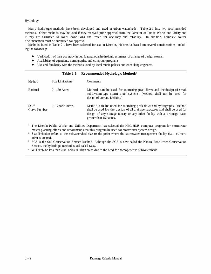
Many hydrologic methods have been developed and used in urban watersheds. Table 2-1 lists two recommendedmethods. Other methods may be used if they received prior approval from the Director of Public Works and Utility andif they are calibrated to local conditions and tested for accuracy and reliability. In addition, complete sourcedocumentation must be submitted for approval.

Methods listed in Table 2-1 have been selected for use in Lincoln, Nebraska based on several considerations, includ-ing the following:

! Verification of their accuracy in duplicating local hydrologic estimates of a range of design storms.! Availability of equations, nomographs, and computer programs. ! Use and familiarity with the methods used by local municipalities and consulting engineers.

Table 2-1 Recommended Hydrologic Methods1

Method Size Limitations2 Comments

Rational 0 - 150 Acres Method can be used for estimating peak flows and the design of smallsubdivision-type storm drain systems. (Method shall not be used fordesign of storage facilities.)

SCS3 0 - 2,000ª Acres Method can be used for estimating peak flows and hydrographs. MethodCurve Number shall be used for the design of all drainage structures and shall be used for

design of any storage facility or any other facility with a drainage basingreater than 150 acres.

1 The Lincoln Public Works and Utilities Department has selected the HEC-HMS computer program for stormwatermaster planning efforts and recommends that this program be used for stormwater system design.

2 Size limitation refers to the subwatershed size to the point where the stormwater management facility (i.e., culvert,inlet) is located.

3 SCS is the Soil Conservation Service Method. Although the SCS is now called the Natural Resources ConservationService, the hydrologic method is still called SCS.

4 Will likely be less than 2000 acres in urban areas due to the need for homogeneous subwatersheds.

Hydrology


2.2 Symbols And Definitions

To provide consistency within this chapter, as well as throughout this manual, the following symbols will be used.These symbols were selected because of their wide use in hydrologic publications.

Table 2-2 Symbols And Definitions

Symbol Definition Units

A Drainage area acres or mi2

C Runoff coefficient -Cf Frequency factor -CN SCS-runoff curve number -d Time interval hoursF Pond and swamp adjustment factor -I Rainfall intensity in./hrIA Percentage of impervious area %Ia Initial abstraction from total rainfall in.NRCS Natural Resources Conservation Service -n Manning’s roughness coefficient -P Accumulated rainfall in.Q Rate of runoff cfsq Storm runoff during a time interval in.R Hydraulic radius ftS or Y Ground slope ft/ft or %S Potential maximum retention storage in.SCS Soil Conservation Service -SL Main channel slope ft/ftSL Standard deviation of the logarithms of the peak annual floods -TB Time base of unit hydrograph hourstc or Tc Time of concentration min or hoursTL Lag time hoursV Velocity ft/s

2.3 Concept Definitions

A good understanding of the following concepts will be important in any hydrologic analysis. These concepts willbe used throughout the remainder of this chapter in dealing with different aspects of hydrologic studies.

Antecedent Moisture Conditions

Antecedent moisture conditions are the soil moisture conditions of the watershed at the beginning of a storm. Theseconditions affect the volume of runoff generated by a particular storm event. Notably they affect the peak discharge inthe lower range of flood magnitudes — say below about the 15-year event threshold. As floods become more rare,antecedent moisture has a rapidly decreasing influence on runoff.

Depression StorageDepression storage is the water stored in natural depressions within a watershed. Generally, after the depression

storage is filled, runoff will commence.

Frequency

Hydrology


The frequency with which a given flood can be expected to occur is the reciprocal of the probability or chance thatthe flood will be equaled or exceeded in a given year. If a flood has a 20 percent chance of being equaled or exceededeach year, over a long period of time, the flood will be equaled or exceeded on an average of once every five years.This is also referred to as the recurrence interval or return period.

Hydraulic Roughness

Hydraulic roughness is a measure of the physical characteristics which impede the flow of water across the earth'ssurface, whether natural or channelized. It affects both the time response of a watershed and drainage channel as wellas the channel storage characteristics.

Hydrograph

A hydrograph is a graph of the time distribution of runoff (expressed as a flow rate) from a watershed.

Hyetographs

The hyetograph is a graph of the time distribution of rainfall (usually expressed as an intensity) over a watershed.

Infiltration

Infiltration is the complex process whereby water penetrates the ground surface and is either stored in the soil porespaces or flows to lower layers. An infiltration curve is a graph of the time distribution at which this occurs.

Interception

Storage of rainfall on foliage and other intercepting surfaces during a rainfall event is called interception storage.

Lag Time

Lag time is defined as the time from the centroid of the excess rainfall to the peak of the hydrograph.

Peak Discharge

The peak discharge, sometimes called peak flow, is the maximum rate of flow of water passing a given point duringor after a rainfall event or snowmelt.

Rainfall Excess

The rainfall excess is the water available to runoff after interception, depression storage and infiltration are satisfied.

Recurrence Interval

The time interval in which an event will occur once on the average. (i.e. a 10-year storm is expected to occur onceevery 10 years, on the average)

Stage

The stage of a river or other water body is the elevation of the water surface above some elevation datum.

Time Of Concentration

The time of concentration is the time it takes a drop of water falling on the hydraulically most remote point in thewatershed to travel through the watershed to the outlet or design point.

Hydrology


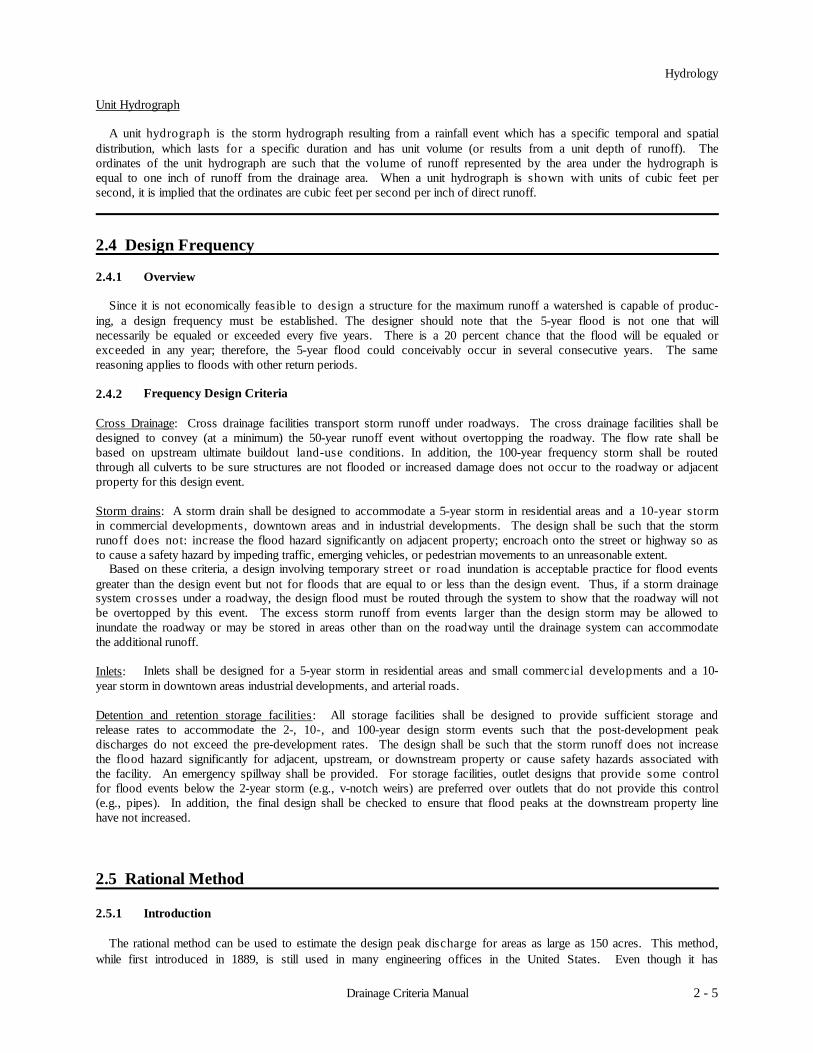
Unit Hydrograph

A unit hydrograph is the storm hydrograph resulting from a rainfall event which has a specific temporal and spatialdistribution, which lasts for a specific duration and has unit volume (or results from a unit depth of runoff). Theordinates of the unit hydrograph are such that the volume of runoff represented by the area under the hydrograph isequal to one inch of runoff from the drainage area. When a unit hydrograph is shown with units of cubic feet persecond, it is implied that the ordinates are cubic feet per second per inch of direct runoff.

2.4 Design Frequency

2.4.1 Overview

Since it is not economically feasible to design a structure for the maximum runoff a watershed is capable of produc-ing, a design frequency must be established. The designer should note that the 5-year flood is not one that willnecessarily be equaled or exceeded every five years. There is a 20 percent chance that the flood will be equaled orexceeded in any year; therefore, the 5-year flood could conceivably occur in several consecutive years. The samereasoning applies to floods with other return periods.

2.4.2 Frequency Design Criteria

Cross Drainage: Cross drainage facilities transport storm runoff under roadways. The cross drainage facilities shall bedesigned to convey (at a minimum) the 50-year runoff event without overtopping the roadway. The flow rate shall bebased on upstream ultimate buildout land-use conditions. In addition, the 100-year frequency storm shall be routedthrough all culverts to be sure structures are not flooded or increased damage does not occur to the roadway or adjacentproperty for this design event.

Storm drains: A storm drain shall be designed to accommodate a 5-year storm in residential areas and a 10-year stormin commercial developments, downtown areas and in industrial developments. The design shall be such that the stormrunoff does not: increase the flood hazard significantly on adjacent property; encroach onto the street or highway so asto cause a safety hazard by impeding traffic, emerging vehicles, or pedestrian movements to an unreasonable extent.

Based on these criteria, a design involving temporary street or road inundation is acceptable practice for flood eventsgreater than the design event but not for floods that are equal to or less than the design event. Thus, if a storm drainagesystem crosses under a roadway, the design flood must be routed through the system to show that the roadway will notbe overtopped by this event. The excess storm runoff from events larger than the design storm may be allowed toinundate the roadway or may be stored in areas other than on the roadway until the drainage system can accommodatethe additional runoff.

Inlets: Inlets shall be designed for a 5-year storm in residential areas and small commercial developments and a 10-year storm in downtown areas industrial developments, and arterial roads.

Detention and retention storage facilities: All storage facilities shall be designed to provide sufficient storage andrelease rates to accommodate the 2-, 10-, and 100-year design storm events such that the post-development peakdischarges do not exceed the pre-development rates. The design shall be such that the storm runoff does not increasethe flood hazard significantly for adjacent, upstream, or downstream property or cause safety hazards associated withthe facility. An emergency spillway shall be provided. For storage facilities, outlet designs that provide some controlfor flood events below the 2-year storm (e.g., v-notch weirs) are preferred over outlets that do not provide this control(e.g., pipes). In addition, the final design shall be checked to ensure that flood peaks at the downstream property linehave not increased.

2.5 Rational Method

2.5.1 Introduction

The rational method can be used to estimate the design peak discharge for areas as large as 150 acres. This method,while first introduced in 1889, is still used in many engineering offices in the United States. Even though it has

Hydrology


frequently come under criticism for its simplistic approach, no other drainage design method has received suchwidespread use.

2.5.2 Concept and Equation

The rational formula estimates the peak rate of runoff at any location in a watershed as a function of the drainagearea, runoff coefficient, and mean rainfall intensity for a duration equal to the time of concentration (the time requiredfor water to flow from the hydraulically most remote point of the basin to the location being analyzed). The rationalformula is expressed as follows:

Q = CIA (2.1)

where: Q = peak rate of runoff, cfsC = runoff coefficient representing a ratio of runoff to rainfall for future land-use conditionsI = average rainfall intensity for a duration equal to the time of concentration, for a selected return period

in./hr (see Figure 2-3)A = drainage area tributary to the design location, acres

2.5.3 Application

Peak discharges estimated using the rational formula are very sensitive to the parameters that are used. The designermust use good engineering judgment in assigning values to these parameters. Each of the parameters used in therational method is discussed below.

2.5.3.1 Time Of Concentration

The time of concentration (tc) is the time required for water to flow from the hydraulically most remote point of thedrainage area to the point under investigation. Use of the rational formula requires the time of concentration (tc) for eachdesign point within the drainage basin. The duration of rainfall is then set equal to the time of concentration and is usedto estimate the rainfall intensity (I). For a storm drain system, the time of concentration consists of an inlet time plusthe time of flow in a closed conduit or open channel to the design point. Inlet time is the time required for runoff to flowover the surface to the nearest inlet and is primarily a function of the length of overland flow, the slope of the land andsurface cover. Pipe or open channel flow time can be estimated from the hydraulic properties of the conduit or channel.One way to estimate overland flow time is to use Figure 2-1 to estimate overland flow velocity and divide the velocityinto the overland travel distance.

For design situations that do not involve complex drainage conditions, Figure 2-2 can be used to estimate inlet time.For each drainage area, the distance is determined from the inlet to the most remote point in the tributary area. Froma topographic map, the average slope is determined for the same distance. The Coefficient of Runoff, C is determinedby the procedure described in a subsequent section of this chapter.

To obtain the total time of concentration, the pipe or open channel flow time must be calculated and added to the inlettime. After first determining the average flow velocity in the pipe or channel, the travel time is obtained by dividingvelocity into the pipe or channel length. Manning's equation can be used to determine velocity. See Chapter 5 - OpenChannel Hydraulics - for a discussion of Manning's equation.

Time of concentration is an important variable in most hydrologic methods. Several methods are available forestimating tc. Appendix 2-C (Travel Time Estimation) at the end of this chapter describes the method from the SCSTechnical Release No. 55 (2nd Edition). Figure 2-2 shows the velocities used for estimating time of concentration forvarious land use conditions. For inlet design the minimum tc recommended should not be less than 8 minutes.

Hydrology


Figure 2-1 Velocities For Estimating Time Of Concentration

Source: HEC No. 19, FHWA

Hydrology


Figure 2-2 Overland Time Of Flow

Source: Airport Drainage, Federal Aviation Administration, 1965

Hydrology


2.5.3.1.1 Common Errors

Two common errors should be avoided when calculating tc. First, in some cases runoff from a portion of the drainagearea which is highly impervious may result in a greater peak discharge than would occur if the entire area wereconsidered. In these cases, adjustments can be made to the drainage area by disregarding those areas where flow timeis too slow to add to the peak discharge. Sometimes it is necessary to estimate several different times of concentrationto determine the design flow that is critical for a particular application.

Second, when designing a drainage system, the overland flow path is not necessarily perpendicular to the contoursshown on available mapping. Often the land will be graded and swales will intercept the natural contour and conductthe water to the streets, which reduces the time of concentration. Care should be exercised in selecting sheet flow pathsin excess of 100 ft in urban areas and 300 ft in rural areas. Sheet flow conditions are not likely to be sustained forgreater lengths and the estimated Tc will be too large.

2.5.3.2 Rainfall Intensity

The rainfall intensity (I) is the average rainfall rate (in./hr) for a duration equal to the time of concentration for aselected return period. Once a particular return period has been selected for design and a time of concentration calculat-ed for the drainage area, the rainfall intensity can be determined from Intensity-Duration-Frequency (IDF) curves. Thedata from the IDF curve for the City of Lincoln are given in Figure 2-3.

Hydrology


Source: Lincoln Public Works and Utilities Department

Hydrology


2.5.3.3 Runoff Coefficient

The runoff coefficient (C) is the variable of the rational method least susceptible to precise determination and requiresjudgment and understanding on the part of the designer. Engineering judgment will always be required in the selectionof runoff coefficients since a typical coefficient represents the integrated effects of many drainage basin parameters.The following discussion considers only the effects of soil groups, land use and average land slope.

The method for determining the runoff coefficient (C) is based on land use, soil groups and land slope. Table 2-4in Manual gives the recommended coefficient C of runoff for pervious surfaces by selected hydrologic soil groupingsand slope ranges. The value of C shall be based on fully built-out land use conditions. The minimum runoff coefficientshall be 0.4 , unless owner can clearly demonstrate that the value less then 0.4 is adequate.

Table 2-4 gives the recommended coefficient C of runoff for pervious surfaces by selected hydrologic soil group-ings and slope ranges. From this table the C values for non-urban areas such as forest land, agricultural land, and openspace can be determined. Soil properties influence the relationship between runoff and rainfall since soils have differingrates of infiltration. Infiltration is the movement of water through the soil surface into the soil. Based on infiltrationrates, the Soil Conservation Service (SCS) has divided soils into four hydrologic soil groups as follows:

Group A Soils having a low runoff potential due to high infiltration rates. These soils consist primarily of deep,well-drained sands and gravels.

Group B Soils having a moderately low runoff potential due to moderate infiltration rates. These soils consistprimarily of moderately deep to deep, moderately well to well-drained soils with moderately fine tomoderately coarse textures.

Group C Soils having a moderately high runoff potential due to slow infiltration rates. These soils consist primarilyof soils in which a layer exists near the surface that impedes the downward movement of water or soils withmoderately fine to fine texture.

Group D Soils having a high runoff potential due to very slow infiltration rates. These soils consist primarily ofclays with high swelling potential, soils with permanently high water tables, soils with a claypan or claylayer at or near the surface and shallow soils over nearly impervious parent material.

A list of soils for the City of Lincoln and their hydrologic classification is presented in the Lancaster County SoilSurvey.

As the slope of the drainage basin increases, the selected C value should also increase. This is caused by the factthat as the slope of the drainage area increases, the velocity of overland and channel flow will increase, allowing lessopportunity for water to infiltrate. Thus, more of the rainfall will become runoff from the drainage area.

It is often desirable to develop a composite runoff coefficient based on the percentage of different types of surface inthe drainage area. Composites can be made with Tables 2-3 and 2-4. The composite procedure can be applied to anentire drainage area or to typical "sample" blocks as a guide to selection of reasonable values of the coefficient for anentire area.

Table 2-3 Recommended Coefficient Of Runoff Values For Various Selected Land Uses

Description of Area Runoff CoefficientsBusiness: Downtown areas 0.70-0.95Neighborhood areas 0.50-0.70Residential: Single-family areas 0.30-0.50

Multi units, detached 0.40-0.60Multi units, attached 0.60-0.75Suburban 0.25-0.40

Residential (1 acre lots or larger) 0.30-0.45Apartment dwelling areas 0.50-0.70Industrial: Light areas 0.50-0.80

Heavy areas 0.60-0.90Parks, cemeteries 0.10-0.25Playgrounds 0.20-0.40Railroad yard areas 0.20-0.40Unimproved areas 0.04-0.38 (see Table 2-4)

Source: Hydrology, Federal Highway Administration, HEC No. 19, 1984

Hydrology


Table 2-4 Recommended Coefficient Of Runoff For Pervious Surfaces (Unimproved Areas)By Selected Hydrologic Soil Groupings And Slope Ranges

Slope A B C DFlat 0.04-0.09 0.07-0.12 0.11-0.16 0.15-0.20(0 - 1%)Average 0.09-0.14 0.12-0.17 0.16-0.21 0.20-0.25(2 - 6%)Steep 0.13-0.18 0.18-0.24 0.23-0.31 0.28-0.38(Over 6%)

Source: Storm Drainage Design Manual, Erie and Niagara Counties Regional Planning Board.

2.5.3.3.1 Infrequent Storm

The coefficients given in Tables 2-3 and 2-4 are applicable for storms of 5-year to 10-year frequencies. Less frequent,higher intensity storms will require modification of the coefficient because infiltration and other losses have a pro-portionally smaller effect on runoff (Wright-McLaughlin, 1969). The adjustment of the rational method for use withmajor storms can be made by multiplying the right side of the rational formula by a frequency factor Cf. The rationalformula now becomes:

Q = CfCIA (2.1)

Cf values are listed in Table 2-5. The product of Cf times C shall not exceed 1.0.

Table 2-5 Frequency Factors For Rational Formula

Recurrence Interval (years) Cf

25 1.150 1.2

100 1.25

2.5.4 Limitations

Some precautions should be considered when applying the rational method.

! The first step in applying the rational method is to obtain a good topographic map and define the boundariesof the drainage area in question. A field inspection of the area should also be made to determine if the naturaldrainage divides have been altered.

! In determining the runoff coefficient (C) value for the drainage area, thought should be given to future changesin land use that might occur during the service life of the proposed facility that could result in an inadequatedrainage system. Also, the effects of permanent upstream detention facilities may be taken into account.

! Restrictions to the natural flow such as highway crossings and dams that exist in the drainage area should beinvestigated to see how they affect the design flows.

! The charts, graphs and tables included in this section are not intended to replace reasonable and prudentengineering judgment which should permeate each step in the design process.

Characteristics of the rational method which limit its use to 150 acres include:

(1) The rate of runoff resulting from any rainfall intensity is a maximum when the rainfall intensity lasts as longor longer than the time of concentration. That is, the entire drainage area does not contribute to the peakdischarge until the time of concentration has elapsed.

Hydrology


This assumption limits the size of the drainage basin that can be evaluated by the rational method. For large drainageareas, the time of concentration can be so large that constant rainfall intensities for such long periods do not occur andshorter, more intense rainfalls can produce larger peak flows.

(2) The frequency of peak discharges is the same as that of the rainfall intensity for the given time of concentra-tion.

Frequencies of peak discharges depend on rainfall frequencies, antecedent moisture conditions in the watershed, andthe response characteristics of the drainage system. For small and largely impervious areas, rainfall frequency is thedominant factor. For larger drainage basins and undeveloped drainage basins, the response characteristics control thefrequencies of peak discharges. For drainage areas with few impervious surfaces (less urban development), antecedentmoisture conditions usually govern, especially for rainfall events with a return period of 10 years or less.

(3) The fraction of rainfall that becomes runoff (C) is independent of rainfall intensity or volume.

This assumption is reasonable for impervious areas, such as streets, rooftops and parking lots. For pervious areas, thefraction of runoff varies with rainfall intensity and the accumulated volume of rainfall. Thus, the “art” necessary forapplication of the rational method involves the selection of a coefficient that is appropriate for the storm, soil and landuse conditions. Many guidelines and tables have been established, but seldom, if ever, have they been supported withempirical evidence.

(4) The rational method provides estimates of only peak discharge rates of runoff. It does not provide informationon the volume of runoff.

Modern drainage practice often includes detention of urban storm runoff to reduce the peak rate of runoff down-stream. With only the peak rate of runoff, the rational method severely limits the evaluation of design alternativesavailable in urban and in some instances, rural drainage design.

Thus, the rational formula is best suited for small, highly impervious areas and least suitable for large drainage areasor drainage areas in natural or undeveloped conditions.

2.5.5 Example Problem - Rational Method

The following example problem illustrates the application of the rational method to estimate peak discharges.Preliminary estimates of the maximum rate of runoff are needed at the inlet to a culvert for a 10-year and 100-yearreturn period.

Site Data

From a topographic map and field survey, the area of the drainage basin upstream from the culvert found to be 18acres. In addition the following data were measured:

Length of overland flow = 50 ftAverage overland slope = 2.0%Length of main basin channel = 1300 ftSlope of channel = 0.018 ft/ft = 1.8%Hydraulic radius = 1.97 ftEstimated roughness coefficient (n) of channel = 0.090

Hydrology


Land Use And Soil Data

From existing land use maps, land use for the drainage basin was estimated to be:

Residential (single family) 80%Undeveloped (2% slope) 20%

For the undeveloped area, the soil group was determined from a SCS map to be:

Group B 100%

From existing land use maps, the land use for the overland flow area at the head of the basin was estimated to be:

Undeveloped (Soil Group B, 2.0% slope) 100%

Overland Flow

A runoff coefficient (C) for the overland flow area was determined to be 0.12 from Table 2-4.

Time Of Concentration

From Figure 2-2, with an overland flow length of 50 ft, slope of 2.0%, and a C of 0.12, the inlet time is 10 min. Channel flow velocity is determined from Manning's formula to be 3.5 ft/s (n = 0.090, R = 1.97 ft and S = 0.018ft/ft). Therefore,

Flow Time = (1300 ft)/(3.5 ft/s)(60 s/min) = 6.2 minand tc = 10 + 6.2 = 16.2 min - say 16 min

Rainfall Intensity

From Figure 2-3 with duration equal to 16 min,

I10 (10-year return period) = 4.50 in./hr

I100 (100-year return period) = 7.05 in./hr

Runoff Coefficient

A weighted runoff coefficient C for the total drainage area is determined in Table 2-6 by utilizing the values fromTables 2-3 and 2-5.

Table 2-6 Weighted Runoff Coefficient, C

(1) (2) (3)Percent Weightedof Total Runoff Runoff

Land Use Land Area Coefficient Coefficient*

Residential(single family) 0.80 0.40 0.32

Undeveloped(Soil Group B) 0.20 0.12 0.02

Total Weighted Runoff Coefficient 0.34

* Column 3 equals column 1 multiplied by column 2.

Hydrology


Peak Runoff

From the rational equation:

Q10 = CIA = 0.34 × 4.50 × 18 = 28 cfs

Q100 = CfCIA = 1.25 × 0.34 × 7.05 × 18 = 54 cfs From Table 2.5

These are the estimates of peak runoff for a 10-year and 100-year design storm for the given basin.

2.6 SCS Unit Hydrograph Method

2.6.1 Introduction

Techniques developed by the U. S. Soil Conservation Service for calculating rates of runoff require the same basicdata as the rational method: drainage area, a runoff factor, time of concentration and rainfall. The SCS approach,however, is more sophisticated in that it considers also the time distribution of the rainfall, the initial rainfall losses tointerception and depression, storage and an infiltration rate that decreases during the course of a storm. With the SCSmethod, the direct runoff can be calculated for any storm, either real or fabricated, by subtracting infiltration and otherlosses from the rainfall to obtain the precipitation excess (runoff volume). Details of the methodology can be found inthe SCS National Engineering Handbook, Section 4.

Two types of hydrographs are used in the SCS procedure, unit hydrographs and dimensionless hydrographs. A unithydrograph represents the time distribution of flow resulting from one inch of direct runoff occurring over the watershedin a specified time. A dimensionless hydrograph represents the composite of many unit hydrographs. The dimension-less unit hydrograph is plotted in nondimensional units of time divided by time to peak and discharge divided by peakdischarge.

Characteristics of the dimensionless hydrograph vary with the size, shape and slope of the tributary drainage area.The most significant characteristics affecting the dimensionless hydrograph shape are the basin lag and the peakdischarge for a given rainfall. Basin lag is the time from the center of mass of rainfall excess to the hydrograph peak.Steep slopes, compact shape and an efficient drainage network tend to make lag time short and peaks high; flat slopes,elongated shape and an inefficient drainage network tend to make lag time long and peaks low.

2.6.2 Concepts and Equations

The following discussion outlines the basic concepts and equations utilized in the SCS method.

2.6.2.1 Rainfall-Runoff

Rainfall-Runoff Equation - A relationship between accumulated rainfall and accumulated runoff was derived bySCS from experimental plots for numerous soils and vegetative cover conditions. Data for land-treatment measures,such as contouring and terracing, from experimental watersheds were included. The equation was developed mainlyfor small watersheds from which only daily rainfall and watershed data are ordinarily available. It was developedfrom recorded storm data that included the total amount of rainfall in a calendar day but not its distribution withrespect to time. The SCS runoff equation is therefore a method of estimating direct runoff from 24-hr or 1-day stormrainfall. The equation is:

Q = (P - Ia)2 / (P - Ia) + S (2.2)

Where: Q = accumulated direct runoff, in.P = accumulated rainfall (potential maximum runoff), in.Ia = initial abstraction including surface storage, interception and infiltration prior to runoff, in.S = potential maximum retention, in.

The relationship between Ia and S was developed from experimental watershed data. It eliminates the need forestimating Ia for common usage. The empirical relationship used in the SCS runoff equation is:

Hydrology


Ia = 0.2S (2.3)

By substituting 0.2S for Ia in equation 2.3, the SCS rainfall-runoff equation becomes:

Q = (P - 0.2S)2 / (P + 0.8S) (2.4)

S is related to the soil and cover conditions of the watershed through the curve number (CN) or runoff factor (SeeSection 2.6.3.1). CN has a range of 0 to 100, and S is related to CN by:

S = (1000 / CN) - 10 (2.5)

Figure 2-4 is a graphical solution of equation 2.4 which enables the precipitation excess (runoff depth) from a stormto be obtained if the total rainfall and watershed curve number are known.

Drainage Area - The drainage area of a watershed is determined from topographic maps and field surveys. For largedrainage areas it might be necessary to divide the area into sub-drainage areas to account for major land use changes,to obtain analysis results at different points within the drainage area, or to locate stormwater drainage facilities andassess their effects on the flood flows. Also a field inspection of existing or proposed drainage systems should be madeto determine if the natural drainage divides have been altered. These alterations could make significant changes in thesize and slope of the subdrainage areas.

Rainfall - The SCS method is based on a 24-hr storm event with various time distributions, depending on thewatershed location. The Type II storm distribution is a "typical" time distribution which the SCS has prepared fromrainfall records and can be used in Lincoln, Nebraska. Figure 2-5 shows this distribution. To use this distribution it isnecessary for the user to obtain the 24-hr duration rainfall value for the frequency of the design storm desired from theTable 2-7.

Table 2-7 City Of Lincoln 24-Hour Design Rainfall

Frequency 24-hour Rainfall Frequency 24-hour Rainfall2-year 3.00 in. 25-year 5.37 in.5-year 3.93 in. 50-year 6.00 in.10-year 4.69 in. 100-year 6.68 in.

Source: National Weather Service, Tech. Paper 40, “Rainfall Frequency Atlas of the U.S.”, May 1961.

2.6.2.2 Time Of Concentration

The average slope within the watershed together with the overall length and retardance of overland flow are the majorfactors affecting the runoff rate through the watershed. In the SCS method, time of concentration (tc) is defined to bethe time required for water to travel from the most hydraulically distant point in a watershed to its outlet. Lag (L) canbe considered as a weighted time of concentration and is related to the physical properties of a watershed, such as area,length and slope. The SCS derived the following empirical relationship between lag and time of concentration:

L = 0.6 tc (2.6)

See Appendix 2-C for information on the derivation of tc.

Hydrology


In small urban areas (less than 2000 acres), a curve number method can be used to estimate the time of concentrationfrom watershed lag. In this method the lag for the runoff from an increment of excess rainfall can be considered as thetime between the center of mass of the excess rainfall increment and the peak of its incremental outflow hydrograph.The equation developed by SCS to estimate lag is:

L = (l0.8 (S + 1)0.7) / (1900 Y0.5) (2.7)

Where: L = lag, hrsl = length of mainstream to farthest divide, ftY = average slope of watershed, %S = (1000/CN) - 10CN = SCS curve number

Hydrology


Figure 2-4 SCS Relation Between Direct Runoff, Curve Number And Precipitation

Source: HEC 19

Hydrology


Figure 2-5 Type II Design Storm Curve

Hydrology


The lag time can be corrected for the effects of urbanization by using Figures 2-6 and 2-7. The amount of modifi-cations to the hydraulic flow length usually must be determined from topographic maps or aerial photographs followinga field inspection of the area. The modification to the hydraulic flow length not only includes pipes and channels butalso the length of flow in streets and driveways.

After the lag time is adjusted for the effects of urbanization, the above equation that relates lag time and time ofconcentration can be used to calculate the time of concentration for use in the SCS method. Appendix 2-c presents analternate procedure for travel time and time of concentration estimation.

2.6.2.3 Triangular Hydrograph Equation

The triangular hydrograph is a practical representation of excess runoff with only one rise, one peak and onerecession. Its geometric makeup can be easily described mathematically, which makes it very useful in the processesof estimating discharge rates. The SCS developed the following equation to estimate the peak rate of discharge for anincrement of runoff:

qp = (484 A (q / (d/2 + L))) (2.8)

Where: qp = peak rate of discharge, cfsA = area, mi2q = storm runoff during time interval, in.d = time interval, hrsL = watershed lag, hrs

This equation can be used to estimate the peak discharge for the unit hydrograph which can then be used to estimatethe peak discharge and hydrograph from the entire watershed.

The constant 484, or peak rate factor, is valid for the SCS dimensionless unit hydrograph. Any change in thedimensionless unit hydrograph reflecting a change in the percent of volume under the rising side would cause acorresponding change in the shape factor associated with the triangular hydrograph and therefore a change in theconstant 484. This constant has been known to vary from about 600 in steep terrain to 300 in very flat, swampy country.

Figure 2-6 Factors For Adjusting Lag When Impervious Areas Occur In Watershed

Source: HEC-19

Hydrology


Figure 2-7 Factors For Adjusting Lag When The Main Channel Has Been Hydraulically Improved

Source: HEC 19

2.6.3 Application

The following discussion describes the procedures used in the SCS unit hydrograph method along with recommendeddesign aids.

2.6.3.1 Runoff Factor

In hydrograph applications, runoff is often referred to as rainfall excess or effective rainfall — all defined as theamount by which rainfall exceeds the capability of the land to infiltrate or otherwise retain the rainfall. The principalphysical watershed characteristics affecting the relationship between rainfall and runoff are land use, land treatment, soiltypes and land slope.

Land use is the watershed cover, and it includes both agricultural and nonagricultural uses. Items such as type ofvegetation, water surfaces, roads, roofs, etc. are all part of the land use. Land treatment applies mainly to agriculturalland use, and it includes mechanical practices such as contouring or terracing and management practices such as rotationof crops.

The SCS uses a combination of soil conditions and land-use (ground cover) to assign a runoff factor to an area. Theserunoff factors, called runoff curve numbers (CN), indicate the runoff potential of an area when the soil is not frozen.The higher the CN, the higher is the runoff potential.

Soil properties influence the relationship between rainfall and runoff by affecting the rate of infiltration. The SCS hasdivided soils into four hydrologic soil groups based on infiltration rates (Groups A, B, C and D). These groups werepreviously described for the rational method. Refer to Lancaster County Soil Survey.

Consideration should be given to the effects of urbanization on the natural hydrologic soil group. If heavy equipmentcan be expected to compact the soil during construction or if grading will mix the surface and subsurface soils,appropriate changes should be made in the soil group selected. Also, runoff curve numbers vary with the antecedent soilmoisture conditions, defined as the amount of rainfall occurring in a selected period preceding a given storm. Ingeneral, the greater the antecedent rainfall, the more direct runoff there is from a given storm. A 5-day period is usedas the minimum for estimating antecedent moisture conditions.

The following pages give a series of tables related to runoff factors. The first tables (Tables 2-8 - 2-10) give curvenumbers for various land uses. These tables are based on an average antecedent moisture condition, i.e., soils that areneither very wet nor very dry when the design storm begins. Curve numbers should be selected only after a fieldinspection of the watershed and a review of zoning and soil maps. Table 2-11 gives conversion factors to convertaverage curve numbers to wet and dry curve numbers. Table 2-12 gives the antecedent conditions for the threeclassifications.

Hydrology


Table 2-8 Runoff Curve Numbers - Urban Areas1

Curve numbers for hydrologic soil groups

Cover type and Average percent A B C Dhydrologic condition impervious area2

Fully developed urban areas (vegetation established)Open space (lawns, parks, golf courses, cemeteries, etc.)3

Poor condition (grass cover <50%) 68 79 86 89Fair condition (grass cover 50% to 75%) 49 69 79 84Good condition (grass cover > 75%) 39 61 74 80

Impervious areas: Paved parking lots, roofs, driveways, etc. (excluding right-of-way) 98 98 98 98

Streets and roads:Paved; curbs and storm drains (excludingright-of-way) 98 98 98 98Paved; open ditches (including right-of-way) 83 89 92 93Gravel (including right-of-way) 76 85 89 91Dirt (including right-of-way) 72 82 87 89

Urban districts: Commercial and business 85% 89 92 94 95 Industrial 72% 81 88 91 93Residential districts by average lot size: 1/8 acre or less (town houses) 65% 77 85 90 92 1/4 acre 38% 61 75 83 87 1/3 acre 30% 57 72 81 86 ½ acre 25% 54 70 80 85 1 acre 20% 51 68 79 84 2 acres 12% 46 65 77 82 Developing urban areas Newly graded areas (pervious areas only, no vegetation) 77 86 91 94Idle lands (CNs are determined using cover types similar to those in Table 2-10).1 Average runoff condition, and Ia = 0.2S

2 The average percent impervious area shown was used to develop the composite CNs. Other assumptions are asfollows: impervious areas are directly connected to the drainage system, impervious areas have a CN of 98, and perviousareas are considered equivalent to open space in good hydrologic condition. If the impervious area is not connected, theSCS method has an adjustment to reduce the effect.

3 CNs shown are equivalent to those of pasture. Composite CNs may be computed for other combinations of open spacecover type.

Source: TR-55

Hydrology


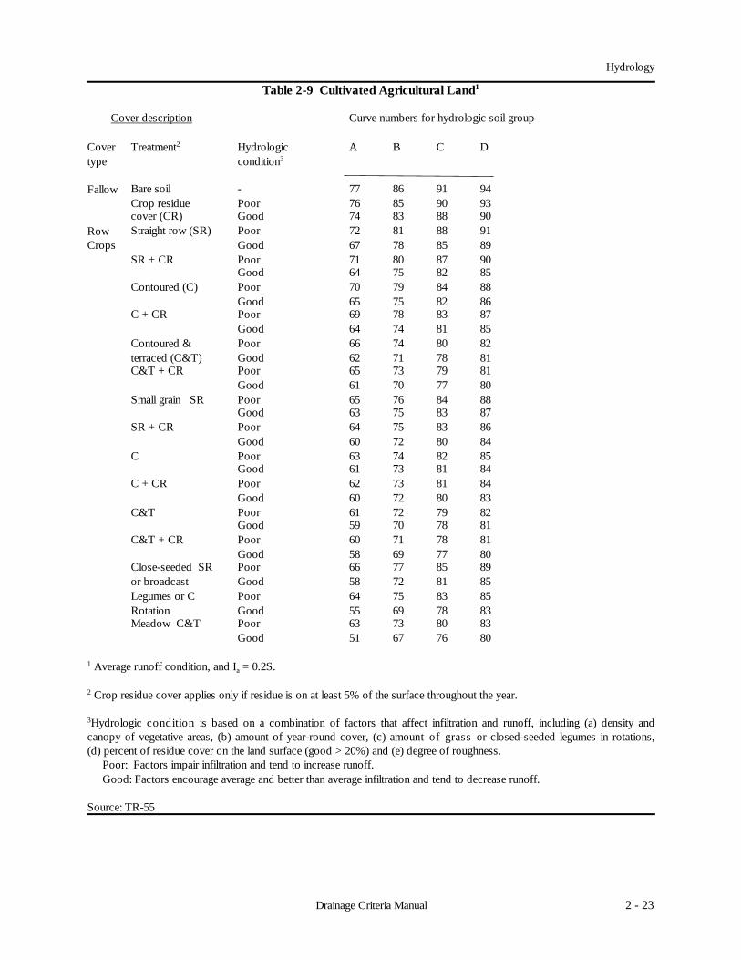
Table 2-9 Cultivated Agricultural Land1

Cover description Curve numbers for hydrologic soil group

Cover Treatment2 Hydrologic A B C Dtype condition3

Fallow Bare soil - 77 86 91 94Crop residue Poor 76 85 90 93cover (CR) Good 74 83 88 90

Row Straight row (SR) Poor 72 81 88 91Crops Good 67 78 85 89

SR + CR Poor 71 80 87 90Good 64 75 82 85

Contoured (C) Poor 70 79 84 88Good 65 75 82 86

C + CR Poor 69 78 83 87Good 64 74 81 85

Contoured & Poor 66 74 80 82terraced (C&T) Good 62 71 78 81C&T + CR Poor 65 73 79 81

Good 61 70 77 80Small grain SR Poor 65 76 84 88

Good 63 75 83 87SR + CR Poor 64 75 83 86

Good 60 72 80 84C Poor 63 74 82 85

Good 61 73 81 84C + CR Poor 62 73 81 84

Good 60 72 80 83C&T Poor 61 72 79 82

Good 59 70 78 81C&T + CR Poor 60 71 78 81

Good 58 69 77 80Close-seeded SR Poor 66 77 85 89or broadcast Good 58 72 81 85Legumes or C Poor 64 75 83 85Rotation Good 55 69 78 83Meadow C&T Poor 63 73 80 83

Good 51 67 76 80

1 Average runoff condition, and Ia = 0.2S.

2 Crop residue cover applies only if residue is on at least 5% of the surface throughout the year.

3Hydrologic condition is based on a combination of factors that affect infiltration and runoff, including (a) density andcanopy of vegetative areas, (b) amount of year-round cover, (c) amount of grass or closed-seeded legumes in rotations,(d) percent of residue cover on the land surface (good > 20%) and (e) degree of roughness. Poor: Factors impair infiltration and tend to increase runoff. Good: Factors encourage average and better than average infiltration and tend to decrease runoff.

Source: TR-55

Hydrology


Table 2-10 Other Agricultural Lands1

Cover description Curve numbers for hydrologic soil group

Cover type Hydrologic A B C D condition

Pasture, grassland, or Poor 68 79 86 89range-continuous forage Fair 49 69 79 84for grazing2 Good 39 61 74 80

Meadow—continuous grass, — 30 58 71 78protected from grazing andgenerally mowed for hay

Brush—brush-weed-grass Poor 48 67 77 83mixture with brush the Fair 35 56 70 77major element3 Good 430 48 65 73

Woods—grass combination Poor 57 73 82 86(orchard or tree farm)5 Fair 43 65 76 82

Good 32 58 72 79

Woods6 Poor 45 66 77 83Fair 36 60 73 79Good 430 55 70 77

Farmsteads—buildings, — 59 74 82 86lanes, driveways and surrounding lots 1 Average runoff condition, and Ia = 0.2S

2 Poor: < 50% ground cover or heavily grazed with no mulch Fair: 50 to 75% ground cover and not heavily grazed Good: > 75% ground cover and lightly or only occasionally grazed

3 Poor: < 50% ground cover Fair: 50 to 75% ground cover Good: > 75% ground cover

4 Actual curve number is less than 30; use CN = 30 for runoff computations.

5 CNs shown were computed for areas with 50% grass (pasture) cover. Other combinations of conditions may becomputed from CNs for woods and pasture.

6 Poor: Forest litter, small trees and brush are destroyed by heavy grazing or regular burning. Fair: Woods grazed but not burned, and some forest litter covers the soil. Good: Woods protected from grazing, litter and brush adequately cover soil.

Source: TR-55

Hydrology


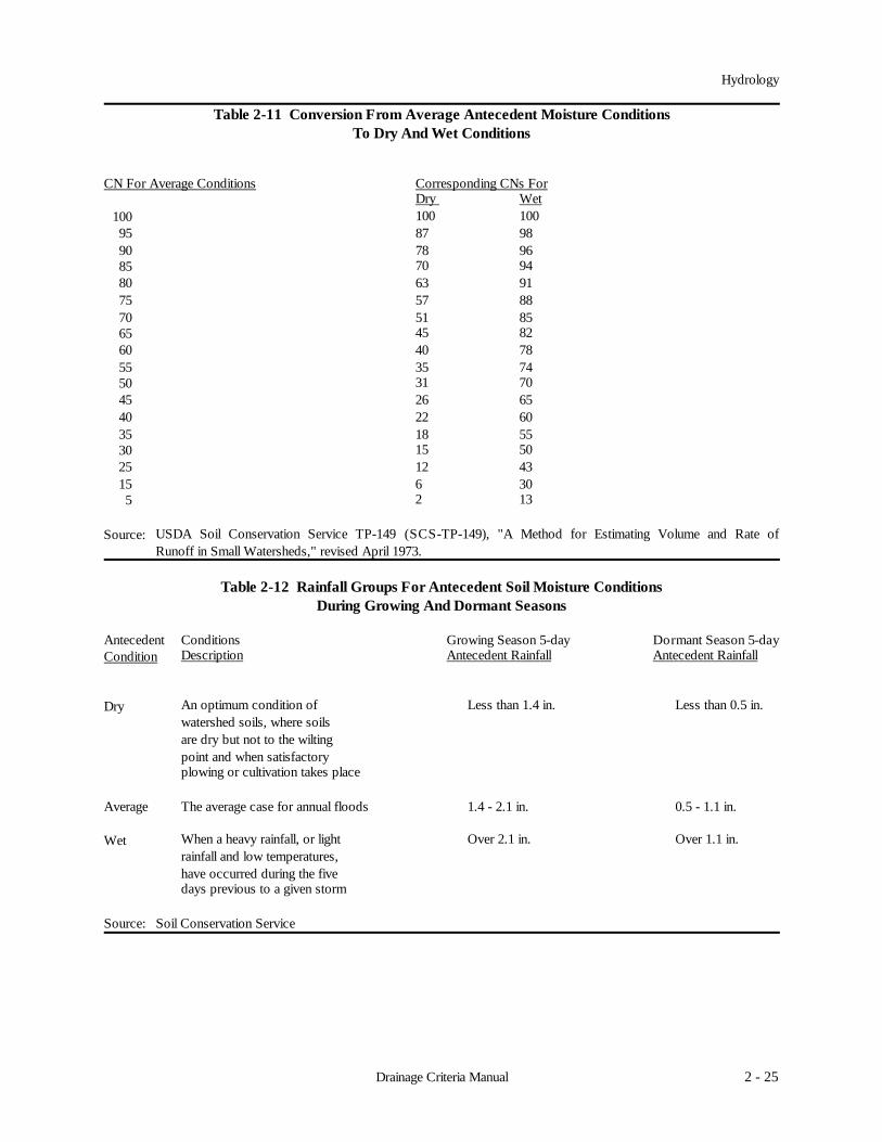
Table 2-11 Conversion From Average Antecedent Moisture ConditionsTo Dry And Wet Conditions

CN For Average Conditions Corresponding CNs ForDry Wet

100 100 10095 87 98

90 78 9685 70 9480 63 9175 57 8870 51 8565 45 8260 40 7855 35 7450 31 7045 26 6540 22 6035 18 5530 15 5025 12 4315 6 305 2 13

Source: USDA Soil Conservation Service TP-149 (SCS-TP-149), "A Method for Estimating Volume and Rate ofRunoff in Small Watersheds," revised April 1973.

Table 2-12 Rainfall Groups For Antecedent Soil Moisture Conditions

During Growing And Dormant Seasons

Antecedent Conditions Growing Season 5-day Dormant Season 5-dayCondition Description Antecedent Rainfall Antecedent Rainfall

Dry An optimum condition of Less than 1.4 in. Less than 0.5 in.

watershed soils, where soils are dry but not to the wiltingpoint and when satisfactory plowing or cultivation takes place

Average The average case for annual floods 1.4 - 2.1 in. 0.5 - 1.1 in.

Wet When a heavy rainfall, or light Over 2.1 in. Over 1.1 in.rainfall and low temperatures,have occurred during the five days previous to a given storm

Source: Soil Conservation Service

Hydrology


2.6.4 Limitations

Several factors, such as the percentage of impervious area and the means of conveying runoff from impervious areasto the drainage system, should be considered in computing CN for urban areas. For example, do the impervious areasconnect directly to the drainage system, or do they outlet onto lawns or other pervious areas where infiltration canoccur?

The curve number values given in Table 2-8 are based on directly connected impervious area. An impervious areais considered directly connected if runoff from it flows directly into the drainage system. It is also considered directlyconnected if runoff from it occurs as concentrated shallow flow that runs over a pervious area and then into a drainagesystem. It is possible that curve number values from urban areas could be reduced by not directly connecting imper-vious surfaces to the drainage system. For a discussion of impervious areas and their effect on curve number values,see Appendix 2-B at the end of this chapter.

2.7 Simplified SCS Method

2.7.1 Introduction

The following SCS procedures were taken from the SCS Technical Release 55 (TR-55) which presents simplifiedprocedures to calculate storm runoff volume, peak rate of discharges and hydrographs. These procedures allow manualcalculation of hydrologic parameters. HEC-HMS performs the same calculations when the SCS methodology isselected within the software package. These procedures are applicable to small drainage areas and include provisionsto account for urbanization. The following procedures outline the use of the SCS-TR 55 method.

2.7.2 Concepts and Equations - Peak Discharge Method

The SCS peak discharge method is applicable for estimating the peak run-off rate from watersheds with homogeneousland uses. The following method is based on the results of computer analyses performed using TR-20, "ComputerProgram for Project Formulation - Hydrology" (SCS 1983).

The peak discharge equation is:

Qp = quAQFp (2.9)

Where:

Qp = peak discharge (cfs)qu = unit peak discharge (cfs/mi2/in.)A = drainage area (mi2)Q = runoff (in.)Fp = pond and swamp adjustment factor

The input requirements for this method are as follows:

1. Time of concentration, Tc (hours)2. Drainage area (mi2)3. Type II rainfall distribution4. 24-hour design rainfall5. CN value6. Pond and swamp adjustment factor (If pond and swamp areas are spread throughout the watershed and are not

considered in the Tc computation, an adjustment is needed.)

Hydrology


Computations for the peak discharge method proceed as follows:

1. The 24-hour rainfall depth is determined from Table 2-7.

2. The runoff curve number, CN, is estimated from Table 2-8 through 2-10 and direct runoff, Q, is calculatedusing equation 2.4.

3. The CN value is used to determine the initial abstraction, Ia, from Table 2-13, and the ratio Ia/P is thencomputed. (P = accumulated rainfall or potential maximum runoff.)

4. The watershed time of concentration is computed using the procedures in Section 2.6.2.2 and is used with theratio Ia/P to obtain the unit peak discharge, qu, from Figure 2-8 or the method given in Appendix 2-C. If theratio Ia/P lies outside the range shown in Figure 2-8, either the limiting values or another peak dischargemethod should be used.

5. The pond and swamp adjustment factor, Fp, is estimated from the following information:

Pond & Swamp Areas (%) Fp Pond & Swamp Areas (%) Fp0 1.00 3.0 0.750.2 0.97 5.0 0.721.0 0.87

6. The peak runoff rate is computed using equation 2.9.

Hydrology


Table 2-13 Ia Values For Runoff Curve Numbers

Curve Number Ia (in) Curve Number Ia (in)40 3.000 70 .85741 2.878 71 .81742 2.762 72 .77843 2.651 73 .74044 2.545 74 .70345 2.444 75 .66746 2.348 76 .63247 2.255 77 .59748 2.167 78 .56449 2.082 79 .53250 2.000 80 .50051 1.922 81 .46952 1.846 82 .43953 1.774 83 .41054 1.704 84 .38155 1.636 85 .35356 1.571 86 .32657 1.509 87 .29958 1.448 88 .27359 1.390 89 .24760 1.333 90 .22261 1.279 91 .19862 1.226 92 .17463 1.175 93 .15164 1.125 94 .12865 1.077 95 .10566 1.030 96 .08367 .985 97 .06268 .941 98 .04169 .899

Hydrology


Figure 2-8 SCS Type II Unit Peak Discharge Graph

Hydrology


2.7.3 Limitations

The accuracy of the peak discharge method is subject to specific limitations, including the following.

1. The watershed must be hydrologically homogeneous and describable by a single/composite CN value.

2. The watershed may have only one main stream, or if more than one, the individual branches must have nearlyequal time of concentrations.

3. Hydrologic routing cannot be considered.

4. The pond and swamp adjustment factor, Fp, applies only to areas located away from the main flow path.

5. Accuracy is reduced if the ratio Ia/P is outside the range given in Figure 2-7.

6. The weighted CN value must be greater than or equal to 40 and less than or equal to 98.

7. The same procedure should be used to estimate pre- and post-development time of concentration whencomputing pre- and post-development peak discharge.

8. The watershed time of concentration must be between 0.1 and 10 hours. 2.7.4 Example Problem

Compute the 25-year peak discharge for a 50-acre wooded watershed which will be developed as follows:

1. Forest land - good cover (hydrologic soil group B) = 10 ac.2. Forest land - good cover (hydrologic soil group C) = 10 ac.3. Town house residential (hydrologic soil group B) = 20 ac.4. Industrial development (hydrological soil group C) = 10 ac.

Other data include:

percentage of pond and swamp area = 0.

The hydrologic flow path for this watershed = 1,920 ft.

Segment Type of Flow Length Slope (%)

1 Overland (n = .45) 70 ft. 2.0 %2 Shallow channel 750 ft. 1.7 %3 Main channel* 1100 ft. 0.20 %

* For the main channel, n = .025, width = 10 feet, depth = 2 feet, rectangular channel.

Computations

1. Calculate rainfall excess:

The 25-year, 24-hour rainfall for Lincoln, Nebraska is 5.37 inches (see Table 2-7).

Hydrology


Composite weighted runoff coefficient is:

Dev. # Area % Total CN Composite CN

1 10 ac. .20 55 11.02 10 ac. .20 70 14.03 20 ac. .40 85 34.04 10 ac. .20 91 18.2

Total 50 ac. 1.00 77.2 use 77

2. Calculate time of concentration (Note: use the method outlined in Appendix 2-C.)

Segment 1 - Travel time from equation 2.C.3 with P2 = 3.00 in.

Tt = [0.42 (0.45 × 70)0.8] / [(3.00)0.5 (.02)0.4]Tt = 18.3 minutes

Segment 2 - Travel time from equation 2.C.5 and equation 2.C.1

V = 2.7 ft/sec (equation 2.C.5)

Tt = 750 / 60 (2.7) = 4.6 minutes

Segment 3 - Using equation 2.C.6 and equation 2.C.1

V = (1.49/.025) (1.43)0.67 (.002)0.5 = 3.4 ft/secTt = 1100 / 60 (3.4) = 5.4 minutes

Tc = 18.3 + 4.6 + 5.4 = 28.3 minutes (.47 hours)

3. Calculate Ia/P

For CN = 77, Ia = .597 (Table 2-13)

Ia/P = (.597 /5.37) = .111(Note: Use Ia/P = .10 to facilitate use of Figure 2-8.

4. Estimate unit discharge qu from Figure 2-8 = 550 cfs/mi2/in

5. Calculate peak discharge with Fp = 1 using equation 2.9

From Figure 2-4 (or equation 2.4), Q = 2.9 inchesQ25 = 550 (50/640) (2.9) (1) = 125 cfs.

2.7.5 Hydrograph Generation

In addition to estimating the peak discharge, the SCS method can be used to estimate the entire hydrograph. The SoilConservation Service has developed a tabular hydrograph procedure which can be used to generate the hydrograph forsmall drainage areas. The tabular hydrograph procedure uses unit discharge hydrographs which have been generatedfor a series of times of concentrations.

Hydrology


The tables in Appendix 2-A at the end of this chapter give the unit discharges (csm/in) for different times ofconcentration which are applicable to the City of Lincoln. The values that should be used are those with a travel timeequal to zero. The other travel times indicate the unit hydrographs which would result if the hydrographs were routedthrough a channel system for a length of time equal to the travel time. Thus, using these unit hydrographs wouldaccount for the effects of channel routing. Straight line interpolation can be used for time of concentrations and traveltimes between the values given in the appendix.

2.7.6 Composite Hydrograph

The procedures given in this chapter are for generation of a hydrograph from a homogeneous developed drainagearea. For drainage areas which are not homogeneous, hydrographs need to be generated from sub-areas and then routedand combined at a point downstream. To accomplish this, engineers should refer to the procedures outlined by the SCSin the 1986 version of TR-55 available from the National Technical Information Service in Springfield, Virginia orwww.usda.nrcs.gov. The catalog number for TR-55, "Urban Hydrology for Small Watersheds," is PB87-101580.

2.7.7 Hydrograph Computation

For the example problem in 2.7.4, calculate the entire hydrograph from the 50 acre development.

Using the chart in Appendix 2-A with a time of concentration of 0.47 hours and Ia/P = 0.10, the following hydrographcan be generated (using straight line interpolation between time of concentration of .4 and .5 hours).

The values given in the charts are in csm/in or cubic feet per second per square mile per inch of runoff. Thus, for thisexample all values from the chart must be multiplied by 0.078 (50 acres/640 acres per square mile), 2.9 inches of runoff,and 1 for the ponding factor - (50/640)(2.9)(1) = 0.23

As an example, from the chart in Appendix 2-A with Tc = 0.47 hours and Ia/P = 0.10, the unit discharge at time 12.1hours is 200 csm/in. Thus, the ordinate on the hydrograph for this example would be 200(.23) = 46 cfs. Thiscalculation must be done for all hydrograph values. The results for selected time values are given in Table 2-14.

Hydrology


Table 2-14 Hydrograph Calculation Results for Selected Time Values

*Hydrograph Time Unit Discharge Hydrograph(hours) (csm/in) (cfs)

11.0 17 411.3 23 511.6 33 811.9 63 1412.0 108 2512.1 200 4612.2 359 8312.3 505 11612.4 544 12512.5 484 11112.6 371 8512.7 273 6312.8 207 4813.0 129 3013.2 91 2113.4 71 1613.6 59 1413.8 52 1214.0 46 1114.3 40 914.6 36 815.0 32 715.5 29 716.0 26 6

* Note skips in time increments.

2.8 Hydrologic Computer Modeling

2.8.1 Introduction

Hydrologic computer models are in widespread use. They are becoming more “user-friendly”, more capable andflexible, and usually provide “report-ready” output. However, a model’s real utility is in monitoring changes in thewatershed or asking “what if” questions. For example, what happens to the 10-year peak discharge as a portion of thewatershed becomes urbanized? Or, alternatively, can the peak discharge be reduced substantially with a strategicallyplaced detention pond? Many hydrologic models will allow one to:

! quantify urban runoff (peaks, volumes, and in some cases, water quality),! obtain design information (channels, pipes, reservoirs, etc.),! determine the effects of control options (infiltration devices, retention ponds, etc.),! perform frequency analysis, and! provide input to economic models.

Hydrology


HEC-HMS (a nonproprietary model written by the U.S. Army Corps of Engineers) has been selected for use inLincoln by the Public Works & Utility Department and the Lower Platte South NRD.

As you begin to use hydrologic computer models, keep in mind the memorable cliché: “Computers are fast, accurate,and stupid. People are slow, inaccurate, and brilliant. The combination is an opportunity beyond imagination.”However, one needs to remain “brilliant” by studying the underlying algorithms these models use. If one knows theirlimitations, he or she can use computer models wisely.

2.8.2 Concepts and Equations

Modern hydrologic models generally require the user to assemble watershed elements on the computer screen in alink-node structure. That is, nodes represent sub-basins (sub-watersheds), confluences (junctions, manholes, etc.),channels/pipes, and reservoirs. These nodes are "linked" together in an arrangement that depicts how runoff passesthrough the watershed.

Mathematical algorithms are associated with each node. For example, a sub-basin node will require certaininformation from the user in order to generate a runoff hydrograph. Rainfall is a necessary input. The user will also berequired to input items like area, curve number, slope, etc. With this information, the model uses internal algorithmsto compute a runoff hydrograph and sends it to the next downstream element. If this element is a channel/pipe node,other data will be required to route the hydrograph to the next element. Reservoir nodes also perform routingcomputations. A confluence node combines two or more hydrographs from upstream sub-basins, channels/pipes, and/orreservoirs. The hydrograph(s) continue to move downstream through all of the watershed elements.

SCS procedures are embedded in most hydrologic models. HEC-HMS allow the user to model watersheds with SCSmethodology. Therefore, the concepts and equations mentioned previously in this chapter are still appropriate. Theseinclude the 24-hour storm, SCS rainfall distributions (like the Type II appropriate for Lincoln), the curve numbermethod for allocating rainfall losses, and the SCS unit hydrograph procedure. 2.8.3 Application

The application of a good hydrologic model is not complicated, particularly if you have a good background inhydrology and a basic understanding of the underlying algorithms used by the model. The step-by-step modelingprocedure listed below is typical of most modern hydrologic models. Of course, the sequence of steps taken and theparticular data requested are dependent upon the model used and the solution methodology (algorithms) chosen.

The step-by-step modeling procedure is likely to progress as follows:

! Launch the model and name your new file.! Choose a system of units, give the project a title, and insert project comments. ! Build a watershed schematic (link/node) using the elements provided on the ?tool palette.”! Choose a solution methodology (e.g., SCS) for individual watershed elements.! Input requested data (e.g., rainfall, curve number, etc.) for each watershed element.! Add any remaining general data (e.g., time step) and run the model. ! Interrogate individual elements from the watershed schematic for output (e.g., hydrographs). ! Evaluate the output data based on sound engineering judgement.! Use the conclusions to determine estimates to the model for reliable output.

2.8.4 Limitations

Hydrologic models are subject to the same limitations as their underlying algorithms. For example, if SCSmodeling procedures are utilized, the precautions and limitations mentioned in section 2.6.4 still apply. The majorlimitations of the SCS methodology are listed below.

! Curve numbers describe average conditions, particularly with regard to antecedent moisture conditions.Since a watershed or sub-watershed is described by one CN value, it should be delineated (to the extentfeasible) such that it is hydrologically homogeneous. (See section 2.7.4 on weighted curve numbers.)

! Initial abstractions are assumed to be 20% of a basin’s potential losses. ! Runoff from snowfall or frozen ground cannot be accounted for using SCS procedures. ! SCS procedures account for surface runoff only, not interflow or groundwater contribution.

Hydrology


Since many hydrologic procedures contain empirical parameters, the processes of calibration and verification can bevery useful in improving model accuracy. These processes require measured rainfall and runoff data from historicalevents. Calibration requires that a watershed be modeled using rainfall information from a number of historical storms.Certain empirical parameters are adjusted in the process so that the modeled output matches the measured output.Verification follows calibration. Using completely different historical rainfall information (not the same storms usedfor calibration), the model is run again with the adjusted empirical parameters to determine the accuracy of the results.If the modeled runoff from these new storms closely matches the measured runoff, the model is assumed to be?verified.” The process of calibration and verification is highly desirable and increases confidence in the results of ahydrologic model.

Hydrology


References

AASHTO Highway Drainage Guidelines, Volume II.

Agency's Regression Equation Study.

Debo, T.N. and A.J. Reese. Municipal Storm Water Management. Boca Raton, Ann Arbor, London, Tokyo: LewisPublishers. 1994

Erie and Niagra Counties Regional Planning Board. Storm Drainage Design Manual.

Federal Highway Administration. HYDRAIN Documentation. 1990.

Newton, D.W., and Herin, Janet C. Assessment of Commonly Used Methods of Estimating Flood Frequency.Transportation Research Board. National Academy of Sciences, Record Number 896. 1982

Overton, D.E. and M.E. Meadows. Storm Water Modeling. Academic Press. New York, N.Y. pp. 58-88. 1976.

Potter, W.D. Upper and Lower Frequency Curves for Peak Rates of Runoff. Transactions, American GeophysicalUnion, Vol. 39, No. 1, pp. 100-105. February 1985.

R.M. Regan. A Nomograph Based on Kinematic Wave Theory for Determining Time of Concentration for OverlandFlow. Report Number 44. Civil Engineering Department, University of Maryland at College Park. 1971

Sauer, V.B., Thomas, W.O., Stricker, V.A., and Wilson, K.V. Flood Characteristics of Urban Watersheds in the UnitedStates — Techniques for Estimating Magnitude and Frequency of Urban Floods. U. S. Geological Survey Water-Supply Paper 2207. 1983.

U.S. Department of Agriculture, Soil Conservation Service. A Method for Estimating Volume and Rate of Runoff inSmall Watersheds, Technical Paper 149. April 1973.

U.S. Department of Agriculture, Soil Conservation Service. National Engineering Handbook, Section 4.

U.S. Department of Agriculture, Soil Conservation Service. Soil Survey of Lancaster County, Nebraska. May 1980.

U.S. Department of Agriculture, Soil Conservation Service. Urban Hydrology for Small Watersheds, Technical Release55. June 1986.

U.S. Department of Transportation, Federal Highway Administration. Hydrology. Hydraulic Engineering Circular No.19. 1984.

Wahl, Kenneth L. Determining Stream Flow Characteristics Based on Channel Cross Section Properties. Transportation Research Board. National Academy of Sciences, Record Number 922. 1983.

Water Resources Council Bulletin 17B. Guidelines for Determining Flood Flow Frequency. 1981.

Urban Drainage and Flood Control District, RED. ED. (1984). Urban Storm Drainage Criteria Manual, Denver RegionalCouncil of Governments, Denver, Colorado.

Appendix 2-A 2-A - 1

Appendix 2-ASCS Unit Discharge Hydrographs

Appendix 2-A2-A - 2


Appendix 2-A2-A - 4


Appendix 2-A2-A - 6


Appendix 2-A2-A - 8


Appendix 2-A2-A - 10


Appendix 2-B 2-B - 1

Appendix 2-BImpervious Area Calculations

2.B.1 Urban Modifications

Several factors, such as the percentage of impervious area and the means of conveying runoff from impervious areasto the drainage system, should be considered in computing the CN for urban areas. For example, do the impervious areasconnect directly to the drainage system, or do they outlet onto lawns or other pervious areas where infiltration can occur?

The curve number values given in Table 2-8 are based on directly connected impervious area. An impervious areais considered directly connected if runoff from it flows directly into the drainage system. It is also considered directlyconnected if runoff from it occurs as concentrated shallow flow that runs over pervious areas and then into a drainagesystem. It is possible that curve number values from urban areas could be reduced by not directly connecting impervioussurfaces to the drainage system. The following discussion will give some guidance for adjusting curve numbers fordifferent types of impervious areas.

Connected Impervious Areas

Urban CNs given in Table 2-8 were developed for typical land use relationships based on specific assumed percentagesof impervious area. These CN values were developed on the assumptions that:

(a) pervious urban areas are equivalent to pasture in good hydrologic condition, and

(b) impervious areas have a CN of 98 and are directly connected to the drainage system.

Some assumed percentages of impervious area are shown in Table 2-8. If all of the impervious area is directly connected to the drainage system, but the impervious area percentages or the

pervious land use assumptions in Table 2-8 are not applicable, use Figure 2-B-1 to compute a composite CN. Forexample, Table 2-8 gives a CN of 70 for a ½-acre lot in hydrologic soil group B, with an assumed impervious area of25 percent. However, if the lot has 20 percent impervious area and a pervious area CN of 61, the composite CN obtainedfrom Figure 2-B-1 is 68. The CN difference between 70 and 68 reflects the difference in percent impervious area.

Unconnected Impervious Areas

Runoff from these areas is spread over a pervious area as sheet flow. To determine CN when all or part of theimpervious area is not directly connected to the drainage system, (1) use Figure 2-B-2 if total impervious area is less then30 percent or (2) use Figure 2-B-1 if the total impervious area is equal to or greater than 30 percent, because theabsorptive capacity of the remaining pervious areas will not significantly affect runoff.

When impervious area is less than 30 percent, obtain the composite CN by entering the right half of Figure 2-B-2 withthe percentage of total impervious area and the ratio of total unconnected impervious area to total impervious area. Thenmove left to the appropriate pervious CN and read down to find the composite CN. For example, for a ½-acre lot with20 percent total impervious area (75 percent of which is unconnected) and pervious CN of 61, the composite CN fromFigure 2-B-2 is 66. If all of the impervious area is connected, the resulting CN (from Figure 2-B-1) would be 68.

Appendix 2-B2-B - 2

Figure 2-B-1 Composite CN With Connected Impervious Areas

Figure 2-B-2 Composite CN With Unconnected Impervious Areas(Total Impervious Area Less Than 30%)

Appendix 2-B 2-B - 3

2.B.2 Composite Curve Numbers

When a drainage area has more than one land use, a composite curve number can be calculated and used in theanalysis. It should be noted that when composite curve numbers are used, the analysis does not take into account thelocation of the specific land uses but sees the drainage area as a uniform land use represented by the composite curvenumber.

Composite curve numbers for a drainage area can be calculated by entering the required data into a table such asTable 2-B-1.

Table 2-B-1 Composite Curve Number Calculations

(1) (2) (3) (4) (5)Land Curve Area % of Total CompositeUse Number Area Curve No.

(Col 2 X Col 4)

The composite curve number for the total drainage area is then the sum of the composite curve numbers fromcolumn 5.

The different land uses within the basin should represent a uniform hydrologic group represented by a single curvenumber. Any number of land uses can be included, but if their spatial distribution is important to the hydrologicanalysis, then sub-basins should be developed and separate hydrographs developed and routed to the study point.

Appendix 2-C 2-C - 1

Appendix 2-CTravel Time Estimation 2.C.1 Introduction

Travel time (Tt) is the time it takes water to travel from one location to another in a watershed. Tt is a component oftime of concentration (Tc), which is the time for runoff to travel from the hydraulically most distant point of the water-shed to a point of interest within the watershed. Tc is computed by summing all the travel times for consecutivecomponents of the drainage conveyance system.

Procedures and equations for calculating travel time and time of concentration are discussed in the following sections.

2.C.2 Travel Time

Water moves through a watershed as sheet flow, shallow concentrated flow, open channel flow, or some combinationof these. The type that occurs is a function of the conveyance system and is best determined by field inspection.

Travel time is the ratio of flow length to flow velocity:

Tt = L/(3600V) (2.C.1)

Where: Tt = travel time, hrL = flow length, ftV = average velocity, ft/s3600 = conversion factor from sec to hrs

2.C.3 Time Of Concentration

The time of concentration is the sum of Tt values for the various consecutive flow segments:

Tc = Tt1 + Tt2 + ... Ttm (2.C.2)

Where: Tc = time of concentration, hrm = number of flow segments

2.C.4 Sheet Flow

Sheet flow is flow over plane surfaces. It usually occurs in the headwater of watersheds. With sheet flow, the frictionvalue (Manning's n) is an effective roughness coefficient that includes the effect of raindrop impact; drag over the planesurface; obstacles such as litter, crop ridges and rocks; and erosion and transportation of sediment. These n values arefor very shallow flow depths of about 0.1 ft or so. Table 2-C-1 gives Manning's n values for sheet flow for varioussurface conditions.

Sheet flow conditions are unlikely for length in excess of 300 ft. In urban residential development, sheet flowconditions may occur in rear yards and other open areas but generally ease when flow occurs between buildings. Forsheet flow use Manning's kinematic solution (Overton and Meadows 1976) to compute Tt:

Tt = [0.42 (nL)0.8 / (P2)0.5s0.4] (2.C.3)

Where: Tt = travel time, minn = Manning's roughness coefficient (Table 2-C-1)L = flow length, ftP2 = 2-year, 24-hr rainfall, in. (3.0 inches in Lincoln)s = slope of hydraulic grade line (land slope), ft/ft

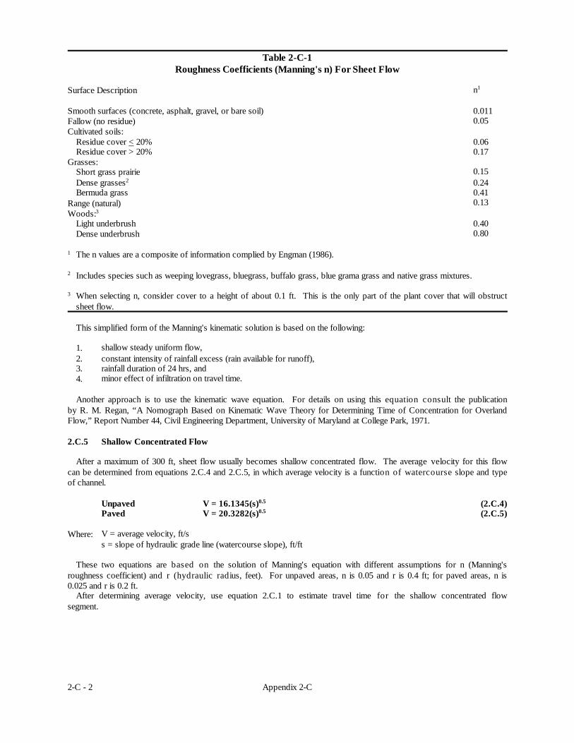
Appendix 2-C2-C - 2

Table 2-C-1Roughness Coefficients (Manning's n) For Sheet Flow

Surface Description n1

Smooth surfaces (concrete, asphalt, gravel, or bare soil) 0.011Fallow (no residue) 0.05Cultivated soils:

Residue cover < 20% 0.06Residue cover > 20% 0.17

Grasses:Short grass prairie 0.15Dense grasses2 0.24Bermuda grass 0.41

Range (natural) 0.13Woods:3

Light underbrush 0.40Dense underbrush 0.80

1 The n values are a composite of information complied by Engman (1986).

2 Includes species such as weeping lovegrass, bluegrass, buffalo grass, blue grama grass and native grass mixtures.

3 When selecting n, consider cover to a height of about 0.1 ft. This is the only part of the plant cover that will obstructsheet flow.

This simplified form of the Manning's kinematic solution is based on the following:

1. shallow steady uniform flow, 2. constant intensity of rainfall excess (rain available for runoff),3. rainfall duration of 24 hrs, and4. minor effect of infiltration on travel time.

Another approach is to use the kinematic wave equation. For details on using this equation consult the publicationby R. M. Regan, “A Nomograph Based on Kinematic Wave Theory for Determining Time of Concentration for OverlandFlow,” Report Number 44, Civil Engineering Department, University of Maryland at College Park, 1971.

2.C.5 Shallow Concentrated Flow

After a maximum of 300 ft, sheet flow usually becomes shallow concentrated flow. The average velocity for this flowcan be determined from equations 2.C.4 and 2.C.5, in which average velocity is a function of watercourse slope and typeof channel.

Unpaved V = 16.1345(s)0.5 (2.C.4)Paved V = 20.3282(s)0.5 (2.C.5)

Where: V = average velocity, ft/ss = slope of hydraulic grade line (watercourse slope), ft/ft

These two equations are based on the solution of Manning's equation with different assumptions for n (Manning'sroughness coefficient) and r (hydraulic radius, feet). For unpaved areas, n is 0.05 and r is 0.4 ft; for paved areas, n is0.025 and r is 0.2 ft.

After determining average velocity, use equation 2.C.1 to estimate travel time for the shallow concentrated flowsegment.

Appendix 2-C 2-C - 3

2.C.6 Open Channels

Open channels are assumed to begin where surveyed cross section information has been obtained, where channels arevisible on aerial photographs, or where blue lines (indicating streams) appear on United States Geological Survey(USGS) quadrangle sheets. Manning's equation or water surface profile information can be used to estimate averageflow velocity. Average flow velocity is usually determined for bank-full elevation. Manning's equation is:

V = (1.49 r2/3 s1/2)/n (2.C.6)

where: V = average velocity, ft/sr = hydraulic radius, ft (equal to a/pw)a = cross sectional flow area, ft2

pw = wetted perimeter, fts = slope of the hydraulic grade line, ft/ftn = Manning's roughness coefficient

After average velocity is computed using equation 2.C.6, Tt for the channel segment can be estimated using equation2.C.1.

2.C.7 Reservoir Or Lake

Sometimes it is necessary to compute a Tc for a watershed which has a relatively large body of water in the flow path.This travel time is normally very small and can be assumed as zero.

One must not overlook the fact that this does not account for the travel time involved with the passage of the inflowhydrograph through spillway storage and the reservoir or lake outlet. This time is generally much longer and is addedto the travel time across the lake. The travel time through lake storage and its outlet can be determined by the storagerouting procedures in Chapter 6. 2.C.8 Limitations

! Manning's kinematic solution should not be used for sheet flow longer than 300 ft. Equation 2.C.3 was devel-oped for use with the four standard SCS rainfall intensity-duration relationships. (i.e., Type II)

! In watersheds with storm drains, carefully identify the appropriate hydraulic flow path to estimate Tc. Stormdrains generally handle only a small portion of a large event. The rest of the peak flow travels by streets, lawns,and so on, to the outlet. Consult Chapter 3 to determine average velocity in pipes for either pressure ornonpressure flow.

! A culvert or bridge can act as a reservoir outlet if there is significant storage behind it. Detailed storage routingprocedures should be used to determine the outflow through the culvert.

Documents

CHAPTER 2 HYDROLOGY 22 February 2000 - lincoln.ne.gov · Hydrology Drainage Criteria Manual 2 - 1 2.1 Overview 2.1.1 Introduction Estimation of the peak rate of runoff, volume of