Embed Size (px)
Citation preview
Chapter 2
Kinematics
2.1 Basic Concepts
Kinematics describes themotionof mechanical systems, without considering theforces that produce that motion. Kinematics deals with velocities and accelerations,which are defined for points of interest on the mechanical systems. The descriptionof motion is relative in nature. Velocities and accelerations are therefore definedwith respect to a reference frame.
2.2 Kinematics of a particle. Rectilinear and curvi-linear motion
The particle is classically represented as a point placed somewhere in space. Arectilinear motionis a straight-line motion. Acurvilinear motionis a motion alonga curved path.
2.2.1 Position vector. Velocity vector. Acceleration vector
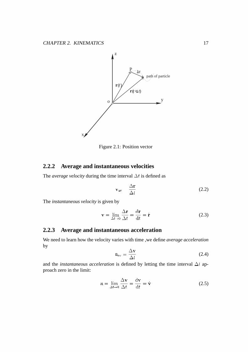
The position vectorr(t) (see Fig. 2.1) of the particle P at a given instant of timet refers to its location relative to some reference point usually taken as the originof a coordinate system. Note that every vector considered in section 2.2 may beprojected onto the coordinate frame oxyz. As the particle moves along its straight-line path, its position changes with time. By definition thedisplacement�r of theparticle during a time interval�t is given by the change of its position during thistime interval.
�r = r(t+�t)� r(t) (2.1)
16
CHAPTER 2. KINEMATICS 17
x
y
z
P
r t( )( )t+ tr
path of particle
o
r
Figure 2.1: Position vector
2.2.2 Average and instantaneous velocities
Theaverage velocityduring the time interval�t is defined as
vav =�r
�t(2.2)
The instantaneous velocityis given by
v = lim�t!0
�r
�t=
dr
dt= _r (2.3)
2.2.3 Average and instantaneous acceleration
We need to learn how the velocity varies with time ,we defineaverage accelerationby
aav =�v
�t(2.4)
and theinstantaneous accelerationis defined by letting the time interval�t ap-proach zero in the limit:
a = lim�t!0
�v
�t=
dv
dt= _v (2.5)
CHAPTER 2. KINEMATICS 18
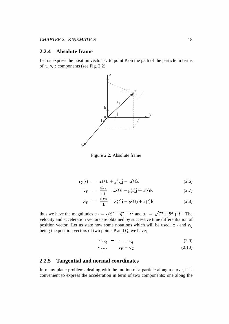
2.2.4 Absolute frame
Let us express the position vectorrP to point P on the path of the particle in termsof x, y, z components (see Fig. 2.2)
x
y
z
r
P
o
P
i
j
k
Figure 2.2: Absolute frame
rP(t) = x(t)i+ y(t)j+ z(t)k (2.6)
vP =drPdt
= _x(t)i+ _y(t)j + _z(t)k (2.7)
aP =dvPdt
= �x(t)i+ �y(t)j + �z(t)k (2.8)
thus we have the magnitudesvP =p
_x2 + _y2 + _z2 andaP =p
�x2 + �y2 + �z2. Thevelocity and acceleration vectors are obtained by successive time differentiation ofposition vector. Let us state now some notations which will be used.rP andrQbeing the position vectors of two points P and Q, we have;
rP=Q = rP � rQ (2.9)
vP=Q = vP � vQ (2.10)
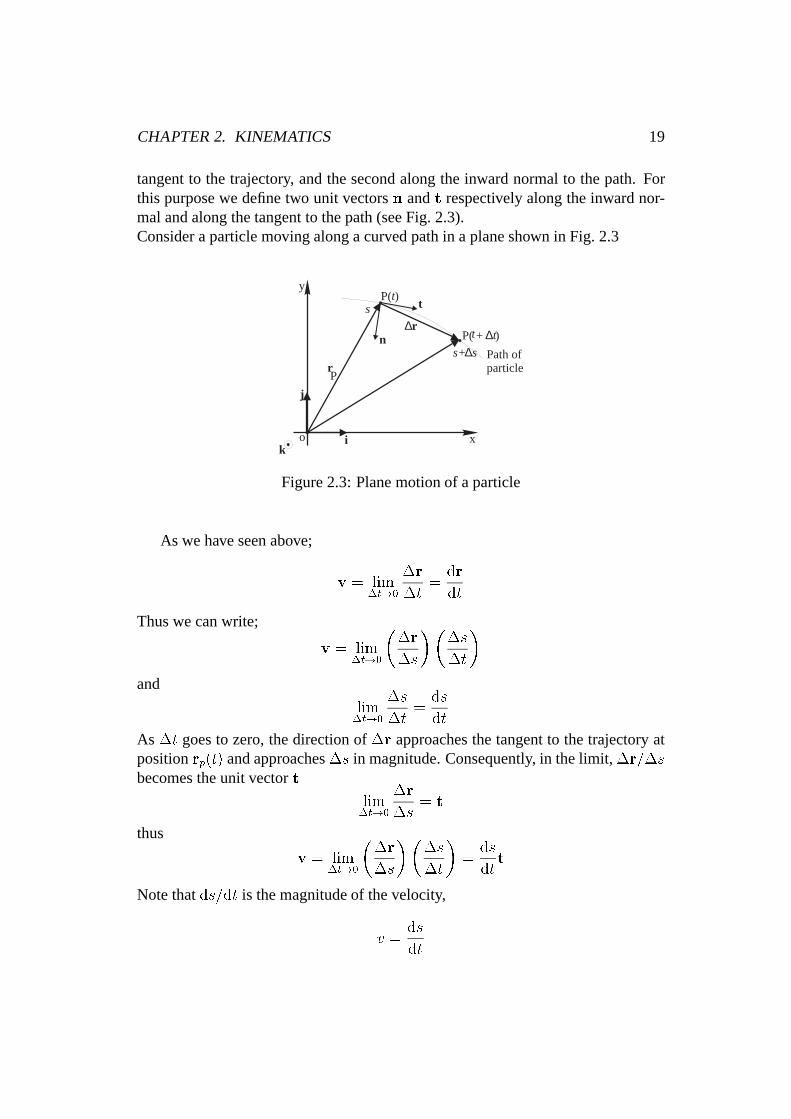
2.2.5 Tangential and normal coordinates
In many plane problems dealing with the motion of a particle along a curve, it isconvenient to express the acceleration in term of two components; one along the
CHAPTER 2. KINEMATICS 19
tangent to the trajectory, and the second along the inward normal to the path. Forthis purpose we define two unit vectorsn andt respectively along the inward nor-mal and along the tangent to the path (see Fig. 2.3).Consider a particle moving along a curved path in a plane shown in Fig. 2.3
Path ofparticle
y
∆∆
∆
xik
rP
sP( )t
t t
o
P( + )s+ s
r
j
t
n
Figure 2.3: Plane motion of a particle
As we have seen above;
v = lim�t!0
�r
�t=
dr
dt
Thus we can write;
v = lim�t!0
��r
�s
���s
�t
�and
lim�t!0
�s
�t=
ds
dt
As �t goes to zero, the direction of�r approaches the tangent to the trajectory atpositionrp(t) and approaches�s in magnitude. Consequently, in the limit,�r=�sbecomes the unit vectort
lim�t!0
�r
�s= t
thus
v = lim�t!0
��r
�s
���s
�t
�=
ds
dtt
Note thatds=dt is the magnitude of the velocity,
v =ds
dt
CHAPTER 2. KINEMATICS 20
Let calculate now the two components of the acceleration
a =dv
dt=
d
dt
�ds
dtt
�
a =d2s
dt2t+
ds
dt
dt
dt=
d2s
dt2t+
ds
dt
dt
ds
ds
dt
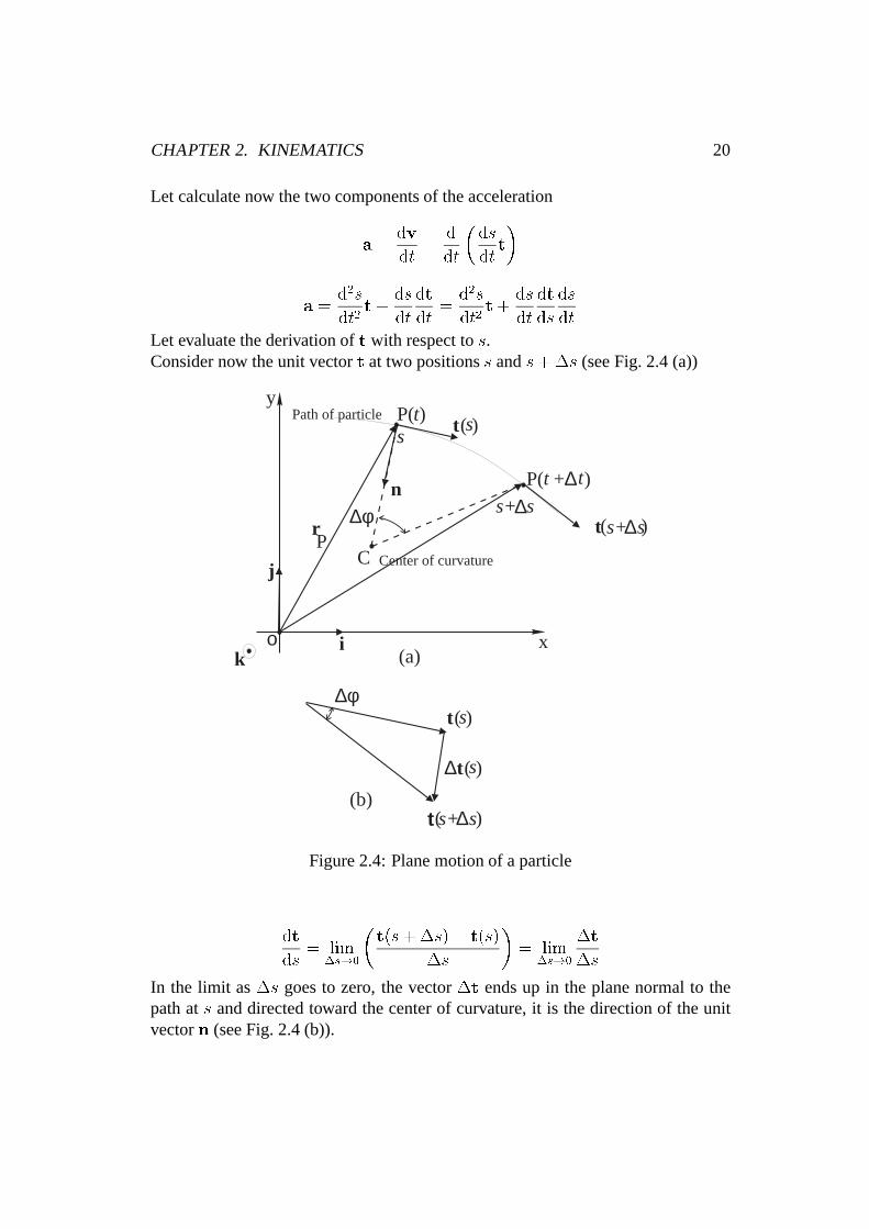
Let evaluate the derivation oft with respect tos.Consider now the unit vectort at two positionss ands+�s (see Fig. 2.4 (a))
Path of particle
Center of curvature
y
∆
∆
∆φ
∆φ
∆∆
∆
xik
r
n
t
t
t
t
t
PC
s
s
s
s+ s
s( )
( )
( )
( )
( )
t
t t
P( )
o
P( + )s+ s
s+ s
j
(a)
(b)
Figure 2.4: Plane motion of a particle
dt
ds= lim
�s!0
�t(s+�s)� t(s)
�s
�= lim
�s!0
�t
�s
In the limit as�s goes to zero, the vector�t ends up in the plane normal to thepath ats and directed toward the center of curvature, it is the direction of the unitvectorn (see Fig. 2.4 (b)).
CHAPTER 2. KINEMATICS 21
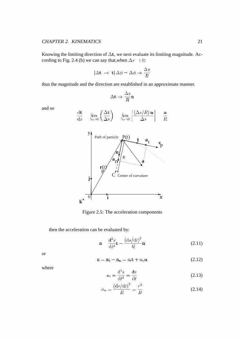
Knowing the limiting direction of�t, we next evaluate its limiting magnitude. Ac-cording to Fig. 2.4 (b) we can say that,when�s! 0:
j�tj ! jtj�� = ��! �s
R
thus the magnitude and the direction are established in an approximate manner.
�t! �s
Rn
and sodt
ds= lim
�s!0
��t
�s
�= lim
�s!0
�(�s=R)n
�s
�=n
R
Path of particle
Center of curvature
y
ik
r
n
t va
aa
P( )
Pt
nR
C
t
t
P( )
o
j
Figure 2.5: The acceleration components
then the acceleration can be evaluated by:
a =d2s
dt2t+
(ds=dt)2
Rn (2.11)
ora = at + an = att+ ann (2.12)
where
at =d2s
dt2=
dv
dt(2.13)
an =(ds=dt)2
R=
v2
R(2.14)
CHAPTER 2. KINEMATICS 22
For a plane curvey = y(x), the radiusR of curvature is given by;
R =
�1 +
�dydx
�2� 3
2��� d2ydx2
��� (2.15)
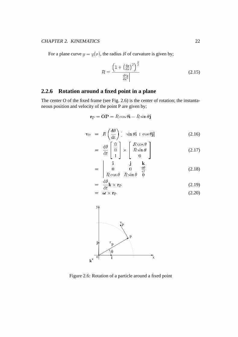
2.2.6 Rotation around a fixed point in a plane
The center O of the fixed frame (see Fig. 2.6) is the center of rotation; the instanta-neous position and velocity of the point P are given by;
rP = OP = R cos �i+R sin �j
vP = R
�d�
dt
�[� sin �i+ cos �j] (2.16)
=d�
dt
24 0
01
35�
24 R cos �
R sin �0
35 (2.17)
=
������i j k
0 0 d�dt
R cos � R sin � 0
������ (2.18)
=d�
dtk� rP (2.19)
= ! � rP (2.20)
y
xik
o
j
v
r
P
P
P
θ
Figure 2.6: Rotation of a particle around a fixed point
CHAPTER 2. KINEMATICS 23
2.3 Kinematics of a rigid body
The description of motion isrelative. Any velocity or acceleration is expressed withregard to a specific reference frame. This fact induces specific notations that mustbe understood:vPS=s denotes the instantaneous velocity of the point P attached tothe body S, relatively to the body s.A rigid bodyis considered to be composed of continuous of distribution of particleshaving fixed distances between each others. There are various types of rigid-bodymotion but the most important of them aretranslationsandrotations.
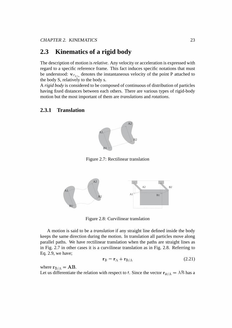
2.3.1 Translation
A1
B1
A2
B2
Figure 2.7: Rectilinear translation
A1
A2
B2
B1
A1
A2
B1
B2
Figure 2.8: Curvilinear translation
A motion is said to be atranslationif any straight line defined inside the bodykeeps the same direction during the motion. In translation all particles move alongparallel paths. We have rectilinear translation when the paths are straight lines asin Fig. 2.7 in other cases it is a curvilinear translation as in Fig. 2.8. Referring toEq. 2.9, we have;
rB = rA + rB=A (2.21)
whererB=A = AB.Let us differentiate the relation with respect tot. Since the vectorrB=A = AB has a
CHAPTER 2. KINEMATICS 24
constant direction and a constant magnitude, its time derivative is zero:
vB = vA
aB = aA
In a translation all particles of the rigid body have same velocity and same acceler-ation.
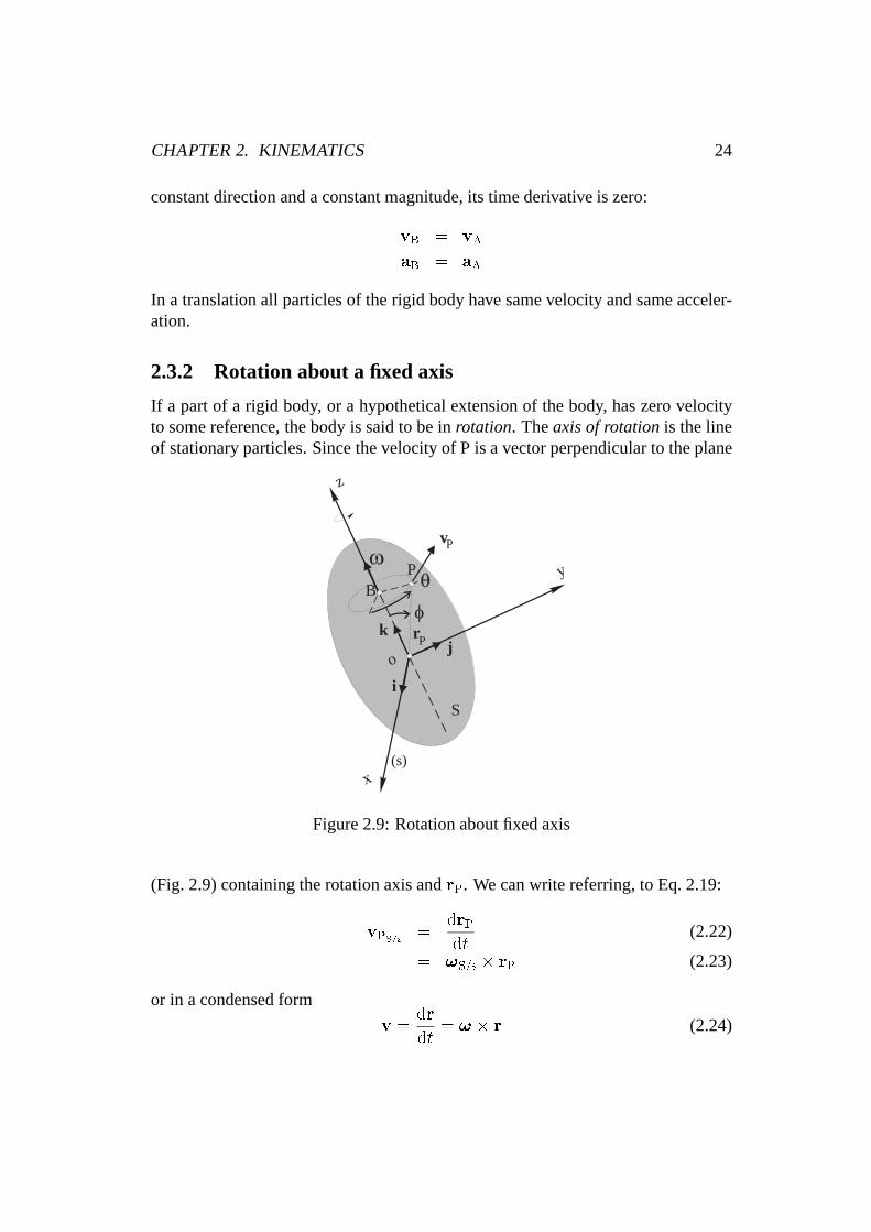
2.3.2 Rotation about a fixed axis
If a part of a rigid body, or a hypothetical extension of the body, has zero velocityto some reference, the body is said to be inrotation. Theaxis of rotationis the lineof stationary particles. Since the velocity of P is a vector perpendicular to the plane
x
y
z
o
i
jk
v
P
S
(s)
P
P
B
r
Figure 2.9: Rotation about fixed axis
(Fig. 2.9) containing the rotation axis andrP. We can write referring, to Eq. 2.19:
vPS=s =drPdt
(2.22)
= !S=s � rP (2.23)
or in a condensed form
v =dr
dt= ! � r (2.24)
CHAPTER 2. KINEMATICS 25
Note that thevector productcan be computed as the determinant:
v =
������vxvyvz
������ =������i j k
!x !y !zx y z
������ (2.25)
And then
vxi = i
���� !y !zy z
���� = i (!yz � y!z)
vyj = �j���� !x !zx z
���� = �j (!xz � x!z)
vzk = k
���� !x !yx y
���� = k (!xy � x!y)
Since! = _�k (2.26)
We have!x = 0, !y = 0, !z = _� and the velocity is completely determined.The accelerationa of P is now determined as
aPS=s =dvPS=sdt
(2.27)
=d
dt
�!S=s � rP
�(2.28)
=d!S=s
dt� rP + !S=s � drP
dt(2.29)
= ��k� rP + !S=s ��!S=s � rP
�(2.30)
2.3.3 Particular case: Motion in plane
A Plane Motionis a motion in which all particles of the body move in parallelplanes.
Velocity in plane motion
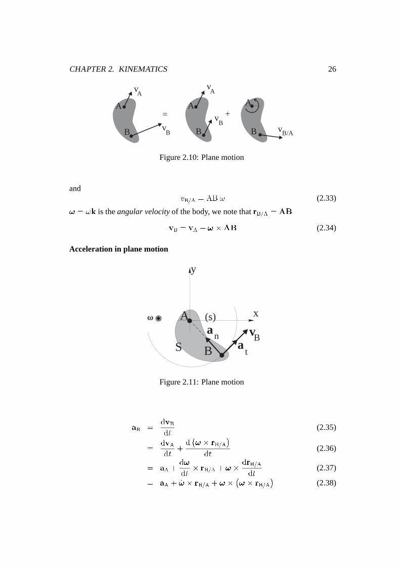
Given two particles A and B of a rigid body in plane motion the velocityvB of B isobtained from the velocity formula (referring to Eq. 2.10)
vB = vA + vB=A (2.31)
In relative motion about A , A is fixed (vA=A = 0). ThusvB=A can be associatedwith the rotation of the body about A and is measured with respect to axes centeredat A
vB=A = ! � rB=A (2.32)
CHAPTER 2. KINEMATICS 26
= +
v
v
v
vvB B
A
AA
B
B
B/A
A
B
A
Figure 2.10: Plane motion
andvB=A = AB ! (2.33)
! = !k is theangular velocityof the body, we note thatrB=A = AB
vB = vA + ! �AB (2.34)
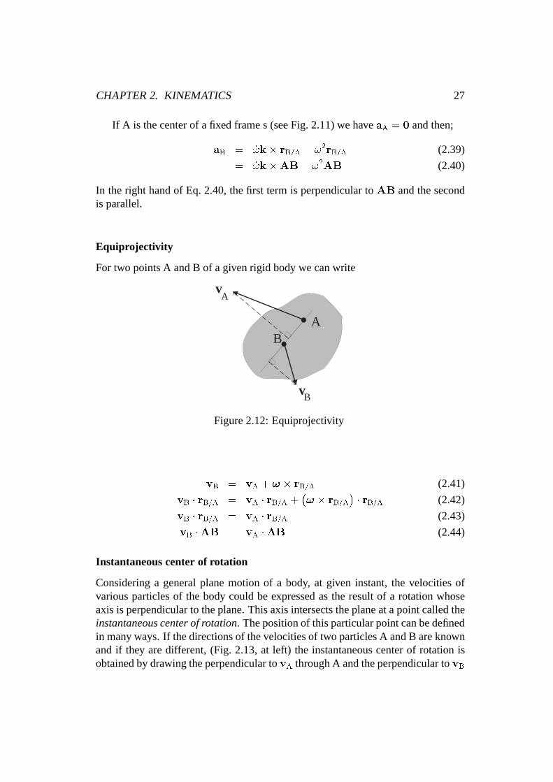
Acceleration in plane motion
BS
(s)
B
t
n va
aA x
y
Figure 2.11: Plane motion
aB =dvBdt
(2.35)
=dvAdt
+d�! � rB=A
�dt
(2.36)
= aA +d!
dt� rB=A + ! � drB=A
dt(2.37)
= aA + _! � rB=A + ! � �! � rB=A�
(2.38)
CHAPTER 2. KINEMATICS 27
If A is the center of a fixed frame s (see Fig. 2.11) we haveaA = 0 and then;
aB = _!k� rB=A � !2rB=A (2.39)
= _!k�AB� !2AB (2.40)
In the right hand of Eq. 2.40, the first term is perpendicular toAB and the secondis parallel.
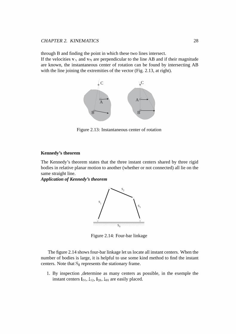
Equiprojectivity
For two points A and B of a given rigid body we can write
A
A
B
B
v
v
Figure 2.12: Equiprojectivity
vB = vA + ! � rB=A (2.41)
vB � rB=A = vA � rB=A +�! � rB=A
� � rB=A (2.42)
vB � rB=A = vA � rB=A (2.43)
vB �AB = vA �AB (2.44)
Instantaneous center of rotation
Considering a general plane motion of a body, at given instant, the velocities ofvarious particles of the body could be expressed as the result of a rotation whoseaxis is perpendicular to the plane. This axis intersects the plane at a point called theinstantaneous center of rotation. The position of this particular point can be definedin many ways. If the directions of the velocities of two particles A and B are knownand if they are different, (Fig. 2.13, at left) the instantaneous center of rotation isobtained by drawing the perpendicular tovA through A and the perpendicular tovB
CHAPTER 2. KINEMATICS 28
through B and finding the point in which these two lines intersect.If the velocitiesvA andvB are perpendicular to the line AB and if their magnitudeare known, the instantaneous center of rotation can be found by intersecting ABwith the line joining the extremities of the vector (Fig. 2.13, at right).
A
B
C
B
A
C
Figure 2.13: Instantaneous center of rotation
Kennedy’s theorem
The Kennedy’s theorem states that the three instant centers shared by three rigidbodies in relative planar motion to another (whether or not connected) all lie on thesame straight line.Application of Kennedy’s theorem
S
S
S
0
1
2
3
S
Figure 2.14: Four-bar linkage
The figure 2.14 shows four-bar linkage let us locate all instant centers. When thenumber of bodies is large, it is helpful to use some kind method to find the instantcenters. Note thatS0 represents the stationary frame.
1. By inspection ,determine as many centers as possible, in the exemple theinstant centersI01, I12, I23, I03 are easily placed.
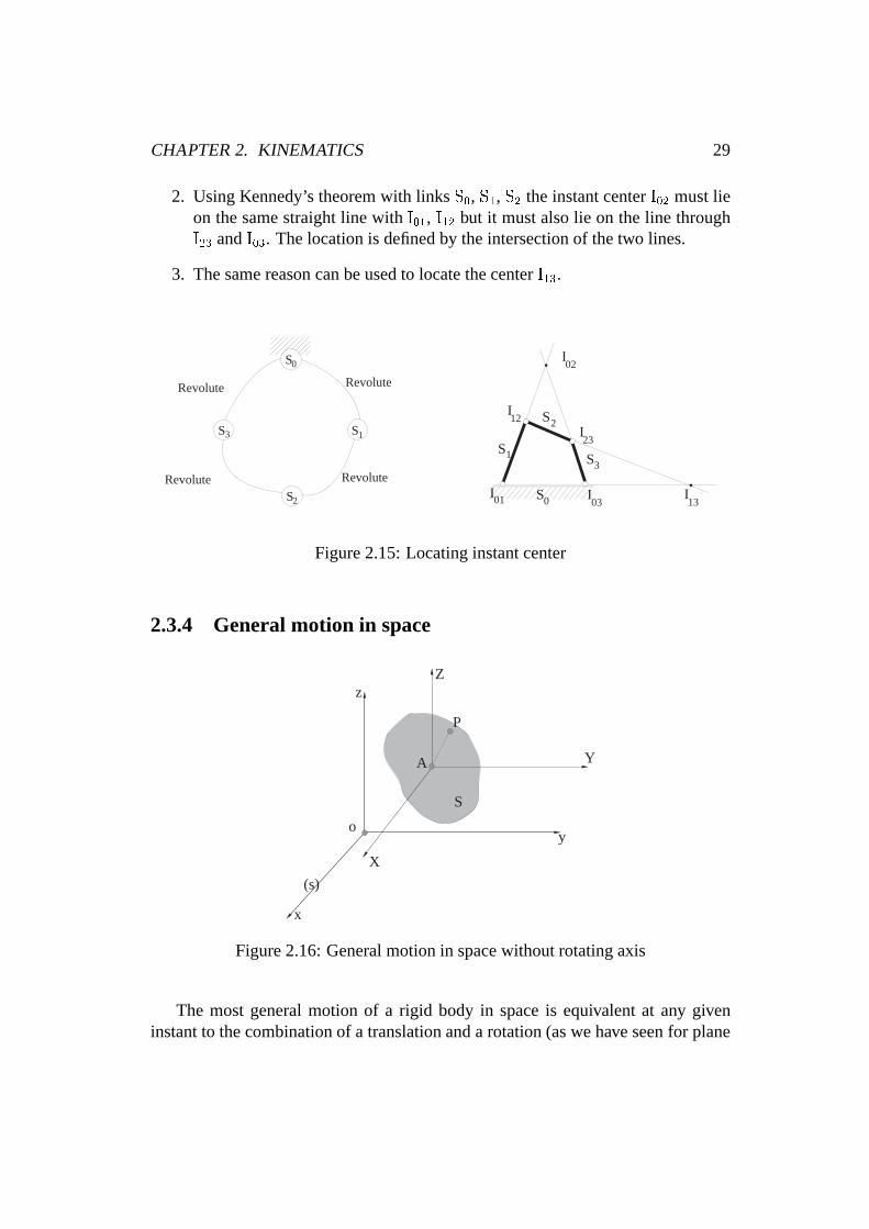
CHAPTER 2. KINEMATICS 29
2. Using Kennedy’s theorem with linksS0, S1, S2 the instant centerI02 must lieon the same straight line withI01, I12 but it must also lie on the line throughI23 andI03. The location is defined by the intersection of the two lines.
3. The same reason can be used to locate the centerI13.
S
SS
S
0
3
2
1
Revolute
Revolute
Revolute
RevoluteS
S
S
S
I I
I
I
I
I0
3
2
1
1303
23
02
12
01
Figure 2.15: Locating instant center
2.3.4 General motion in space
x
y
zZ
X
Y
o
A
P
(s)
S
Figure 2.16: General motion in space without rotating axis
The most general motion of a rigid body in space is equivalent at any giveninstant to the combination of a translation and a rotation (as we have seen for plane
CHAPTER 2. KINEMATICS 30
motion). Considering two particles A and P of the rigid body S, we have:
vP = vA + vP=A (2.45)
WherevP=A is the velocity of P relative to a frame attached to A, thusvP=A =!S=s � rP=A or vP=A = !S=s � AP where! is the angular velocity of the bodyS relative to the fixed frame s. The absolute velocity of a particle P belong to S isgiven by from above:
vPS=s = vAS=s + !S=s �AP (2.46)
The equation 2.46 allows the determination of the velocity of any point P of a bodyS with respect to another frame s,vPS=s, if the following variables are known:
� vAS=s: velocity of a point A of the body S with respect to s.
� !S=s: angular velocity of S with respect to s.
� AP: position of the particle P with respect to A.
The acceleration of P is obtained by differentiating the equation with respect totime.
aPS=s =dvPdt
(2.47)
=dvAP=sdt
+d�!S=s �AP
�dt
(2.48)
= aAS=s + _! �AP+ !S=s � dAP
dt(2.49)
= aA=s + _!S=s �AP+ !S=s ��!S=s �AP
�(2.50)
The equation 2.50 allows the determination of the acceleration of any point P of abody S with respect to another frame s,aPS=s, if the following variables are known:
� aAS=s : acceleration of the point A of the body S with respect to s.
� !S=s: angular velocity of S with respect to s.
� _!S=s: angular acceleration of S with respect to s.
� AP: position of the particle P with respect to A.
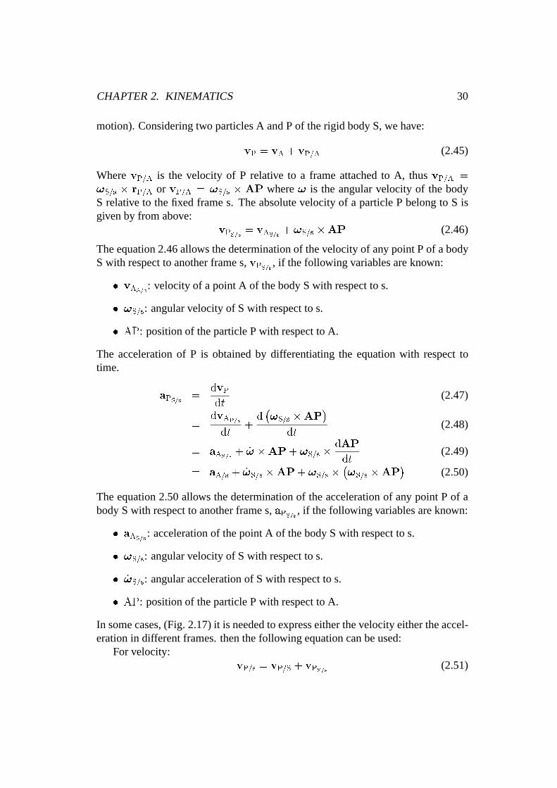
In some cases, (Fig. 2.17) it is needed to express either the velocity either the accel-eration in different frames. then the following equation can be used:
For velocity:vP=s = vP=S + vPS=s (2.51)
CHAPTER 2. KINEMATICS 31
x
y
z
Z
X
Y
o
A
P
(s)
S
Figure 2.17: General motion of a rigid body in space with rotating axis
assume to S and s are two frames, note that herevPS=s represents the velocity of theframe S with respect to the frame s.The acceleration is then given by:
aP=s = aP=S + aPS=s + acor (2.52)
whereacor is the Coriolis acceleration:
acor = 2!S=s � vP=S (2.53)
The Coriolis acceleration has a zero value if:
� the point P has no relative velocity with respect to S (vP=S = 0);
� the relative velocityvP=S = 0 is parallel to the angular velocity!S=s.
(see [2] for demonstration)
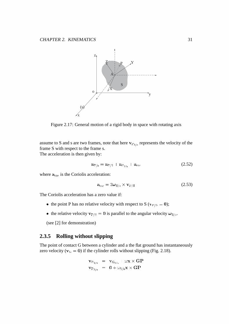
2.3.5 Rolling without slipping
The point of contact G between a cylinder and a the flat ground has instantaneouslyzero velocity (vG = 0) if the cylinder rolls without slipping (Fig. 2.18).
vPS=s = vGS=s + !x�GP
vPS=s = 0+ !S=sx�GP
CHAPTER 2. KINEMATICS 32
o
x
y
z P
A
X
Y
Z
G
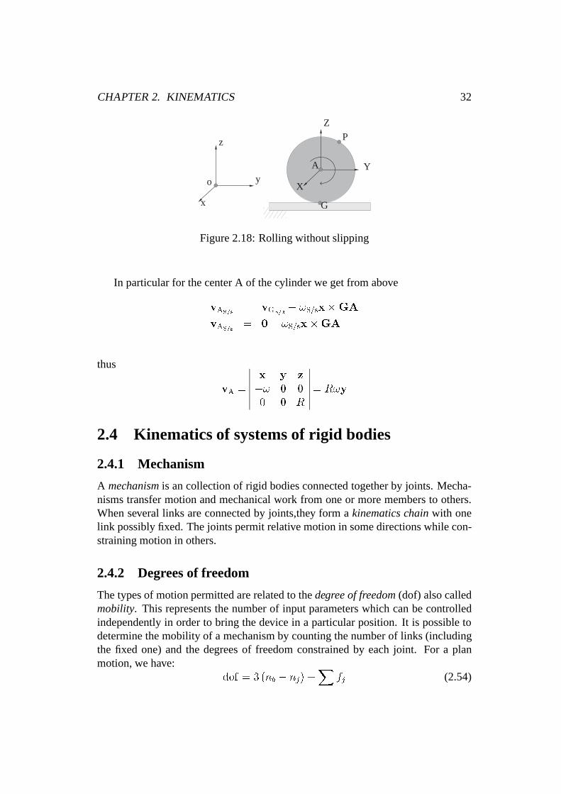
Figure 2.18: Rolling without slipping
In particular for the center A of the cylinder we get from above
vAS=s = vGS=s � !S=sx�GA
vAS=s = 0� !S=sx�GA
thus
vA =x y z
�! 0 00 0 R
= R!y
2.4 Kinematics of systems of rigid bodies
2.4.1 Mechanism
A mechanismis an collection of rigid bodies connected together by joints. Mecha-nisms transfer motion and mechanical work from one or more members to others.When several links are connected by joints,they form akinematics chainwith onelink possibly fixed. The joints permit relative motion in some directions while con-straining motion in others.
2.4.2 Degrees of freedom
The types of motion permitted are related to thedegree of freedom(dof) also calledmobility. This represents the number of input parameters which can be controlledindependently in order to bring the device in a particular position. It is possible todetermine the mobility of a mechanism by counting the number of links (includingthe fixed one) and the degrees of freedom constrained by each joint. For a planmotion, we have:
dof = 3 (nb � nj) +X
fj (2.54)
CHAPTER 2. KINEMATICS 33
where
� nb is the total number of rigid bodies including the fixed link;
� nj is the total number of joints possibly including the fixed link
� fj degree of freedom of relative motion between the bodies constrained bythe kinematical joint.
For a three-dimensional motion
dof = 6 (nb � nj) +X
fj (2.55)
2.4.3 Lower pairs and higher pairs
Namej
Rigidjoint
Revolute
Prismatic
Helical
Cylindrical
Spherical
Planar
0 rotation0 translation
1 rotation0 translation
0 rotation1 translation
1 rotation1 translation
1 rotation1 translation
(right)(left)
3 rotations0 translation
1 rotation2 translations
0
1
1
1
2
2
3
Relativemotion
Degree offreedom (f )
Skecthsymbol
Otherview
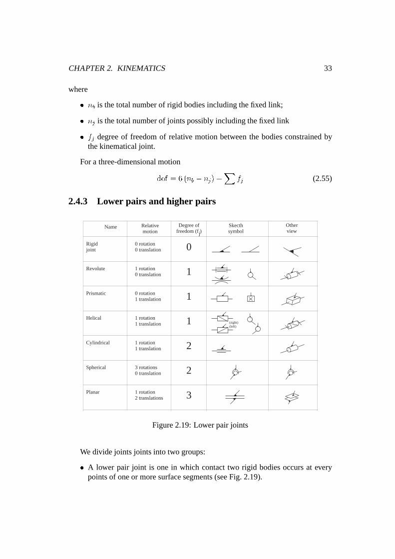
Figure 2.19: Lower pair joints
We divide joints joints into two groups:
� A lower pair joint is one in which contact two rigid bodies occurs at everypoints of one or more surface segments (see Fig. 2.19).
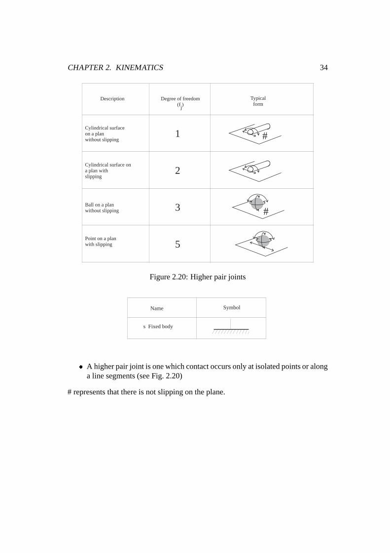
CHAPTER 2. KINEMATICS 34
Description
Cylindrical surfaceon a planwithout slipping
Cylindrical surface ona plan withslipping
Ball on a planwithout slipping
j
Point on a planwith slipping
1
2
3
5
Degree of freedom(f )
Typicalform
#
#
Figure 2.20: Higher pair joints
s Fixed body
Name Symbol
� A higher pair joint is one which contact occurs only at isolated points or alonga line segments (see Fig. 2.20)
# represents that there is not slipping on the plane.
CHAPTER 2. KINEMATICS 35
2.4.4 Kinematics exercises
The MATLAB file Kexx.m can be executed by typingKexx in the interactive windowof MATLAB . It provides an interface where the user may examine the numericalaspects of the exercises simply by pressing command buttons, corresponding to thevarious kinematics exercises. Each button calls the corresponding MATLAB filewith an illustration of the exercise solution. It is also possible to see the solution ofeach exercise by calling the corresponding file, directly from the command line.
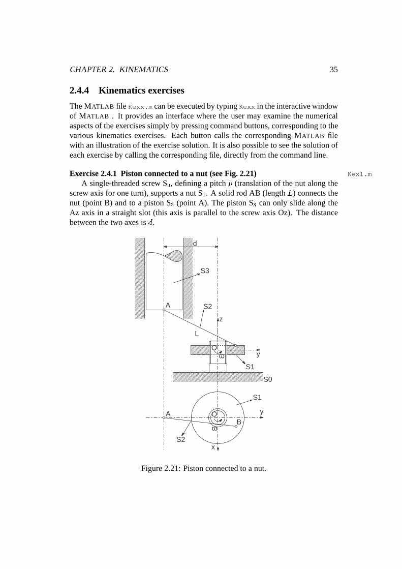
Exercise 2.4.1 Piston connected to a nut (see Fig. 2.21) Kex1.m
A single-threaded screw S0, defining a pitchp (translation of the nut along thescrew axis for one turn), supports a nut S1. A solid rod AB (lengthL) connects thenut (point B) and to a piston S3 (point A). The piston S3 can only slide along theAz axis in a straight slot (this axis is parallel to the screw axis Oz). The distancebetween the two axes isd.
xxxxxxxxxxxxxxxxxxxxxxxxxxxxxxxxxxxxxxxxxxxxxxxxxxxxxxxxxxxxxxxxxxxxxxxxxxxxxxxxxxxxxxxxxxxxxxxxxxxxxxxxxxxxxxxxxxxxxxxxxxxxxxxxxxxxxxxxxxxxxxxxxxxxxxxxxxxxxxxxxxxxxxxxxxxxxxxxxxxxxxxxxxxxxxxxxxxxxxxxxxxxxxxxxxxxxxxxxxxxxxxxxxxxxxxxxxxxxxxxxxxxxxxxxxxxxxxxxxxxxxxxxxxxxxxxxxxxxxxxxxxxxxxxxxxxxxxxxxxxxxxxxxxxxxxxxxxxxxxxxxxxxxxxxxxxxxxxxxxxxxxxxxxxxxxxxxxxxxxxxxxxxxxxxxxxxxxxxxxxxxxxxxxxxxxxxxxxxxxxxxxxxxxxxxxxxxxxxxxxxxxxxxxxxxxxxxxxxxxxxxxxxxxxxxxxxxxxxxxxxxxxxxxxxxxxxxxxxxxxxxxxxxxxxxxxxxxxxxxxxxxxxxxxxxxxxxxxxxxxxxxxxxxxxxxxxxxxxxxxxxxxxxxxxxxxxxxxxxxxxxxxxxxxxxxxxxxxxxxxxxxxxxxxxxxxxxxxxxxxxxxxxxxxxxxxxxxxxxxxxxxxxxxxxx
xxxxxxxxxxxxxxxxxxxxxxxxxxxxxxxxxxxxxxxxxxxxxxxxxxxxxxxxxxxxxxxxxxxxxxxxxxxxxxxxxxxxxxxxxxxxxxxxxxxxxxxxxxxxxxxxxxxxxxxxxxxxxxxxxxxxxxxxxxxxxxxxxxxxxxxxxxxxxxxxxxxxxxxxxxxxxxxxxxxxxxxxxxxxxxxxxxxxxxxxxxxxxxxxxxxxxxxxxxxxxxxxxxxxxxxxxxxxxxxxxxxxxxxxxxxxxxxxxxxxxxxxxxxxxxxxxxxxxxxxxxxxxxxxxxxxxxxxxxxxxxxxxxxxxxxxxxxxxxxxxxxxxxxxxxxxxxxxxxxxxxxxxxxxxxxxxxxxxxxxxxxxxxxxxxxxxxxxxxxxxxxxxxxxxxxxxxxxxxxxxxxxxxxxxxxxxxxxxxxxxxxxxxxxxxxxxxxxxxxxxxxxxxxxxxxxxxxxxxxxxxxxxxxxxxxxxxxxxxxxxxxxxxxxxxxxxxxxxxxxxxxx
xxxxxxxxxxxxxxxxxxxxxxxxxxxxxxxxxxxxxxxxxxxxxxxxxxxxxxxxxxxxxxxxxxxxxxxxxxxxxxxxxxxxxxxxxxxxxxxxxxxxxxxxxxxxxxxxxxxxxxxxxxxxxxxxxxxxxxxxxxxxxxxxxxxxxxxxxxxxxxxxxxxxxxxxxxxxxxxxxxxxxxxxxxxxxxxxxxxxxxxxxxxxxxxxxxxxxxxxxxxxxxxxxxxxxxxxxxxxxxxxxxxxxxxxxxxxxxxxxxxxxxxxxxxxxxxxxxxxxxxxxxxxxxxxxxxxxxxxxxxxxxxxxxxxxxxxxxxxxxxxxxxxxxxxxxxxxxxxxxxxxxxxxxxxxxxxxxxxxxxxxxxxxxxxxxxxxxxxxxxxxxxxxxxxxxxxxxxxxxxxxxxxxxxxxxxxxxxxxxxxxxxxxxxxxxxxxxxxxxxxxxxxxxxxxxxxxxxxxxxxxxxxxxxxxxxxxxxxxxxxxxxxxxxxxxxxxxxxxxxxxxxx
xxxxxxxxxxxxxxxxxxxxxxxxxxxxxxxxxxxxxxxxxxxxxxxxxxxxxxxxxxxxxxxxxxxxxxxxxxxxxxxxxxxxxxxxxxxxxxxxxxxxxxxxxxxxxxxxxxxxxxxxxxxxxxxxxxxxxxxxxxxxxxxxxxxxxxxxxxxxxxxxxxxxxxxxxxxxxxxxxxxxxxxxxxxxxxxxxxxxxxxxxxxxxxxxxxxxxxxxxxxxxxxxxxxxxxxxxxxxxxxxxxxxxxxxxxxxxxxxxxxxxxxxxxxxxxxxxxxxxxxxxxxxxxxxxxxxxxxxxxxxxxxxxxxxxxxxxxxxxxxxxxxxxxxxxxxxxxxx
d
A
L
z
y
S1
S0
ωO
S2
y
x
ω
OAB
S3
S2
xxxxxxxxxxxxxxxxxxxxxxxxxxxxxxxxxxxxxxxxxxxxxxxxxxxxxxxxxxxxxxxxxxxxxxxxxxxxxxxxxxxxxxxxxxxxxxxxxxxxxxxxxxxxxxxxxxxxxxxxxxxxxxxxxxxxxxxxxxxxxxxxxxxxxxxxxxxxxxxxxxxxx
S1
Figure 2.21: Piston connected to a nut.
CHAPTER 2. KINEMATICS 36
The coordinates of A are(0;�d; zA).The coordinates of B are(R cos�;R sin�; p=2��).
If the nut rotates at the constant angular speed! = d�=dt, what is the verticalvelocityvA of the piston?For the following parameters :R = 30 mm, d = 50 mm,L = 10 mm, p = 100 mm,! = 1 rad=s, compute the vertical velocity, with respect to� and compare it withthe results provided by theKex1.m file.
Solution
� The velocityvA is the first time derivative of the coordinatezA. We will firstdetermine the expression ofzA.
AB = AO+OB = OB�OA
=�R cos�;+R sin� + d;
p
2��� zA
�AB2 = L2
= R2 cos� +R2 sin� + d2 + 2Rd sin� +�p�2�� zA
�2�p�2�� zA
�2= L2 �R2 � d2 � 2Rd sin�
zA = �pL2 � R2 � d2 � 2Rd sin�+
p
2��
There are two different solutions but the only physically valid solution iszA>p�/2�.
� Determination ofvAz
vAz =dzAdt
=+��2Rd cos�d�
dt
�2pL2 � R2 � d2 � 2Rd sin�
+p
2�
d�
dt
vAz =�!Rd sin�p
L2 �R2 � d2 � 2Rd sin�+
p
2�!
Another way to solve the problem is presented here.
� First, the velocityvB is determined.
vB = vO + ! �OB
) vO =p
2�!
) vB =�0; 0;
p
2�!�+
������i j k
0 0 !R cos� R sin� 0
������vB =
��!R sin�; !R cos�;
p
2�!�
CHAPTER 2. KINEMATICS 37
� Equiprojectivity along AB is then used:
AB � vAAB=s = AB � vBAB=swith vBAB=s = vBS1=s =
��R sin�!;R cos�!;
p
2�!�
AB =�R cos�;R sin� + d;
p
2�� zA
�vAAB=s = (0; 0; vAz)
) vAz� p
2��� zA
�= �R2 sin� cos�! +R2 sin� cos�!
+Rd cos�! +p
2�!
) vAz =Rd cos�!p2��� zA
+p
2�! (2.56)
) vAz =Rd cos�!
p2��� p
2���pL2 � R2 � d2 � 2Rd sin�
+p
2�! (2.57)
) vAz =p
2�! � Rd cos�!p
L2 � R2 � d2 � 2Rd sin�(2.58)
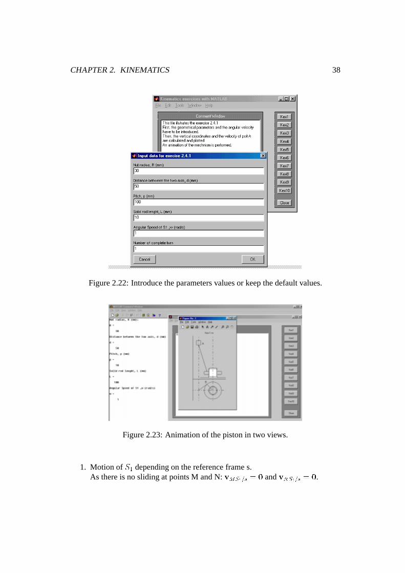
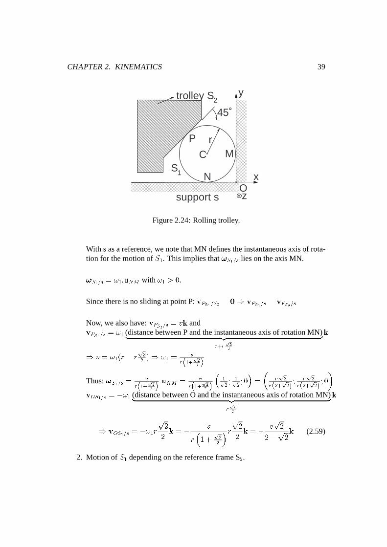
The fileKex1.m illustrates the exercise. First, the geometrical parameters of thesystem (R, d, L, p), the angular velocity and the number of rotations for S1 have tobe introduced (see Fig. 2.22). Then, the vertical coordinates and the velocity of thepoint A are calculated and plotted. An animation of the mechanism is performed(see Fig. 2.23). The mechanical system is shown in different configurations whenthe solid S1 turns around the Oz axis.
Exercise 2.4.2 Rolling trolley (see Fig. 2.24) Kex2.m
A trolley S2, supported by multiple rigid steel balls S1 (radiusr), can only havea rectilinear motion along the conductor rail s (z axis).
It is assumed that there is no sliding at the contact points M, N et P (see Fig. 2.24).If the velocityv = vk of the trolley is known, and if O is considered as a point
of S1, determine, with respect to parametersv andr:
1. the relative velocity of the point O depending on the reference frame s;
2. the relative velocity of the point O depending on the reference frame S2.
For the following parameters:r = 10 mm, v = 10 m=s, compute the relative ve-locities of O depending on the reference frame s, and depending on the referenceframeS2 compare them with the results provided by theKex2.m file.Solution
CHAPTER 2. KINEMATICS 38
Figure 2.22: Introduce the parameters values or keep the default values.
Figure 2.23: Animation of the piston in two views.
1. Motion ofS1 depending on the reference frame s.As there is no sliding at points M and N:vMS1=s = 0 andvNS1=s = 0.
CHAPTER 2. KINEMATICS 39
xxxxxxxxxxxxxxxxxxxxxxxxxxxxxxxxxxxxxxxxxxxxxxxxxxxxxxxxxxxxxxxxxxxxxxxxxxxxxxxxxxxxxxxxxxxxxxxxxxxxxxxxxxxxxxxxxxxxxxxxxxxxxxxxxxxxxxxxxxxxxxxxx
xxxxxxxxxxxxxxxxxxxxxxxxxxxxxxxxxxxxxxxxxxxxxxxxxxxxxxxxxxxxxxxxxxxxxxxxxxxxxxxxxxxxxxxxxxxxxxxxxxxxxxxxxxxxxxxxxxxxxxxxxxxxxxxxxx
xxxxxxxxxxxxxxxxxxxxxxxxxxxxxxxxxxxxxxxxxxxxxxxxxxxxxxxxxxxxxxxxxxxxxxxxxxxxxxxxxxxxxxxxxxxxxxxxxxxxxxxxxxxxxxxxxxxxxxxxxxxxxxxxxxxxxxxxxxxxxxxxxxxxxxxxxxxxxxxxxxxxxxxxxxxxxxxxxxxxxxxxxxxxxxxxxxxxxxxxxxxxxxxxxxxxxxxxxxxxxxxxxxxxxxxxxxxxxxxxxxxxxxxxxxxxxxxxxxxxxxxxxxxxxxxxxxxxxxxxxxxxxxxxxxxxxxxxxxxxxxxxxxxxxxxxxxxxxxxxxxxxxxxxxxxxxxxxxxxxxxxxxxxxxxxxxxxxxxxxxxxxxxxxxxxxxxxxxxxxxxxxxxxxxxxxxxxxxxxxxxxxxxxxxxxxxxxxxxxxxxxxxxxxxxxxxxxxxxxxxxxxxxxxxxxxxxxxxxxxxxxxxxxxxxxxxxxxxxxxxxxxxxxxxxxxxxxxxxxxxxxxxxxxxxxxxxxxxxxxxxxxxxxxxxxxxxxxxxxxxxxxxxxxxxxxxxxxxxxxxxxxxxxxxxxxxxxxxxxxxxxxxxxxxxxxxxxxxxxxxxxxxxxxxxxxxxxxxxxxxxxxxxxxxxxxxxxxxxxxxxxxxxxxxxxxxxxxxxxxxxxxxxxxxxxxxxxxxxxxxxxxxxxxxxxxxxxxxxxxxxxxxxxxxxxxxxxxxxxxxxxxxxxxxxxxxxxxxxxxxxxxxxxxxxxxxxxxxxxxxxxxxxxxxxxxxxxxxxxxxxxxxxxxxxxxxxxxxxxxxxxxxxxxxxxxxxxxxxxxxxxxxxxxxxxxxxxxxxxxxxxxxxxxxxxxxxxxxxxxxxxxxxxxxxxxxxxxxxxxxxxxxxxxxxxxxxxxxxxxxxxxxxxxxxxxxxxxxxxxxxxxxxxxxxxxxxxxxxxxxxxxxxxxxxxxxxxxxxxxxxxxxxxxxxxxxxxxxxxxxxxxxxxxxxxxxxxxxxxxxxxxxxxxxxxxxxxxxxxxxxxxxxxxxxxxxxxxxxxxxxxxxxxxxxxxxxxxxxxxxxxxxxxxxxxxxxxxxxxxxxxxxxxxxxxxxxxxxxxxxxxxxxxxxxxxxxxxxxxxxxxxxxxxxxxxxxxxxxxxxxxxxxxxxxxxxxxxxxxxxxxxxxxxxxxxxxxxxxxxxxxxxxxxxxxxxxxxxxxxxxxxxxxxxxxxxxxxxxxxxxxxxxxxxxxxxxxxxxxxxxxxxxxxxxxxxxxxxxxxxxxxxxxxxxxxxxxxxxxxxxxxxxxxxxxxxxxxxxxxxxxxxxxxxxxxxxxxxxxxxxxxxxxxxxxxxxxxxxxxxxxxxxxxxxxxxxxxxxxxxxxxxxxxxxxxxxxxxxxxxxxxxxxxxxxxxxxxxxxxxxxxxxxxxxxxxxxxxxxxxxxxxxxxxxxxxxxxxxxxxxxxxxxxxxxxxxxxxxxxxxxxxxxxxxxxxxxxxxxxxxxxxxxxxxxxxxxxxxxxxxxxxxxxxxxxxxxxxxxxxxxxxxxxxxxxxxxxxxxxxxxxxxxxxxxxxxxxxxxxxxxxxxxxxxxxxxxxxxxxxxxxxxxxxxxxxxxxxxxxxxxxxxxxxxxxxxxxxxxxxxxxxxxxxxxxxxxxxxxxxxxxxxxxxxxxxxxxxxxxxxxxxxxxxxxxxxxxxxxxxxxxxxxxxxxxxxxxxxxxxxxxxxxxxxxxxxxxxxxxxxxxxxxxxxxxxxxxxxxxxxxxxxxxxxxxxxxxxxxxxxxxxxxxxxxxxxxxxxxxxxxxxxxxxxxxxxxxxxxxxxxxxxxxxxxxxxxxxxxxxxxxxxxxxxxxxxxxxxxxxxxxxxxxxxxxxxxxxxxxxxxxxxxxxxxxxxxxxxxxxxxxxxxxxxxxxxxxxxxxxxxxxxxxxxxxxxxxxxxxxxxxxxxxxxxxxxxxxxxxxxxxxxxxxxxxxxxxxxxxxxxxxxxxxxxxxx
Cr
M
N
P
S1
trolley S2
support sOx zxx
x
x
y
45˚
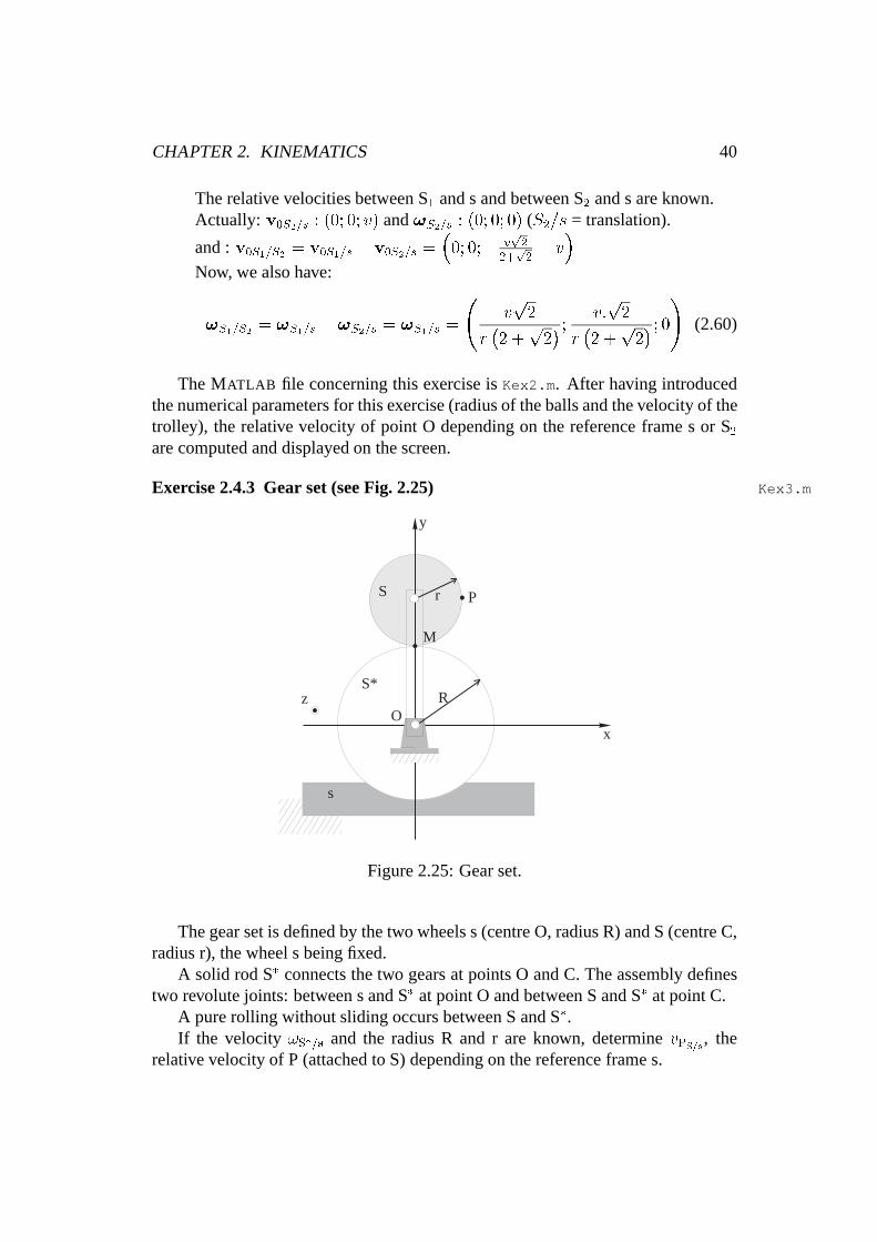
Figure 2.24: Rolling trolley.
With s as a reference, we note that MN defines the instantaneous axis of rota-tion for the motion ofS1. This implies that!S1=s lies on the axis MN.
!S1=s = !1:uNM with !1 > 0.
Since there is no sliding at point P:vPS1=S2 = 0) vPS1=s = vPS2=s
Now, we also have:vPS2=s = vk andvPS1=s = !1 (distance between P and the instantaneous axis of rotation MN)| {z }
r+rp2
2
k
) v = !1(r + rp22)) !1 =
v
r�1+
p2
2
�
Thus:!S1=s =v
r�1+
p2
2
� :uNM = v
r�1+
p2
2
��
1p2; 1p
2; 0�=
�v:p2
r(2+p2); v:
p2
r(2+p2); 0
�vOS1=s = �!1 (distance between O and the instantaneous axis of rotation MN)| {z }
rp2
2
k
) vOS1=s = �!1rp2
2k = � v
r�1 +
p22
�rp2
2k = � v
p2
2 +p2k (2.59)
2. Motion ofS1 depending on the reference frame S2.
CHAPTER 2. KINEMATICS 40
The relative velocities between S1 and s and between S2 and s are known.Actually: v0S2=s : (0; 0; v) and!S2=s : (0; 0; 0) (S2=s = translation).
and :v0S1=S2 = v0S1=s � v0S2=s =�0; 0;� v
p2
2+p2� v�
Now, we also have:
!S1=S2 = !S1=s � !S2=s = !S1=s =
vp2
r�2 +
p2� ; v:
p2
r�2 +
p2� ; 0!
(2.60)
The MATLAB file concerning this exercise isKex2.m . After having introducedthe numerical parameters for this exercise (radius of the balls and the velocity of thetrolley), the relative velocity of point O depending on the reference frame s or S2
are computed and displayed on the screen.
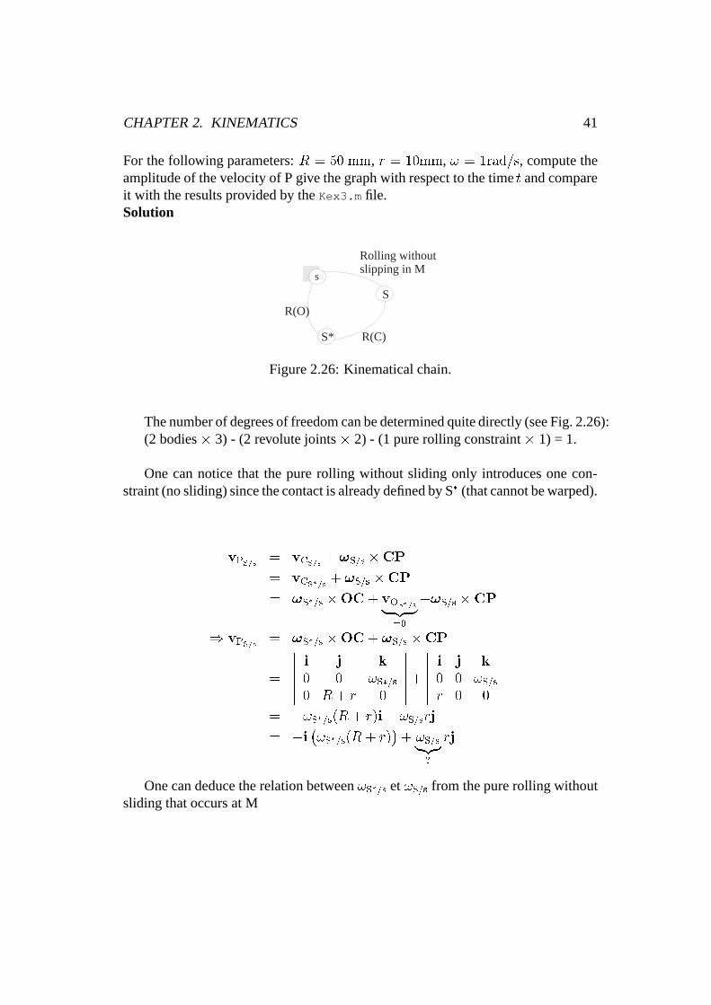
Exercise 2.4.3 Gear set (see Fig. 2.25) Kex3.m
r
s
R
P
M
S
S*
O
y
z
x
Figure 2.25: Gear set.
The gear set is defined by the two wheels s (centre O, radius R) and S (centre C,radius r), the wheel s being fixed.
A solid rod S� connects the two gears at points O and C. The assembly definestwo revolute joints: between s and S� at point O and between S and S� at point C.
A pure rolling without sliding occurs between S and S�.If the velocity !S�=s and the radius R and r are known, determinevPS=s, the
relative velocity of P (attached to S) depending on the reference frame s.
CHAPTER 2. KINEMATICS 41
For the following parameters:R = 50 mm, r = 10mm, ! = 1rad=s, compute theamplitude of the velocity of P give the graph with respect to the timet and compareit with the results provided by theKex3.m file.Solution
s
S
S*
Rolling withoutslipping in M
R(C)
R(O)
Figure 2.26: Kinematical chain.
The number of degrees of freedom can be determined quite directly (see Fig. 2.26):(2 bodies� 3) - (2 revolute joints� 2) - (1 pure rolling constraint� 1) = 1.
One can notice that the pure rolling without sliding only introduces one con-straint (no sliding) since the contact is already defined by S� (that cannot be warped).
vPS=s = vCS=s + !S=s �CP
= vCS�=s + !S=s �CP
= !S�=s �OC+ vOS�=s| {z }=0
+!S=s �CP
) vPS=s = !S�=s �OC+ !S=s �CP
=
������i j k
0 0 !S�=s0 R + r 0
������+������i j k
0 0 !S=sr 0 0
������= �!S�=s(R + r)i+ !S=srj
= �i �!S�=s(R + r)�+ !S=s|{z}
?
rj
One can deduce the relation between!S�=s et!S=s from the pure rolling withoutsliding that occurs at M
CHAPTER 2. KINEMATICS 42
vMS=s= vCS=s + !S=s �CM = 0 (2.61)
= vCS�=s + !S=s �CM (2.62)
= !S�=s �OC+ !S=s �CM (2.63)
) !S�=s �OC+ !S=s �CM = 0 (2.64)
�!S�=s: jOCj :i+ !S=s:r:i = 0 (2.65)
!S=s = !S�=s:R + r
r(2.66)
) vPS=s = �!S�=s(R + r)i+ !S�=s(R + r)j (2.67)
) vPS=s ? MP (2.68)
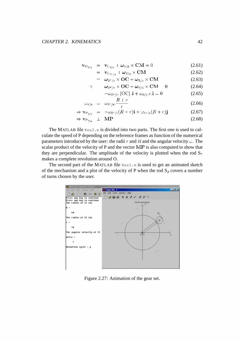
The MATLAB file Kex3.m is divided into two parts. The first one is used to cal-culate the speed of P depending on the reference frames as function of the numericalparameters introduced by the user: the radiir andR and the angular velocity!. Thescalar product of the velocity of P and the vectorMP is also computed to show thatthey are perpendicular. The amplitude of the velocity is plotted when the rod S2
makes a complete revolution around O.The second part of the MATLAB file Kex3.m is used to get an animated sketch
of the mechanism and a plot of the velocity of P when the rod S2 covers a numberof turns chosen by the user.
Figure 2.27: Animation of the gear set.
CHAPTER 2. KINEMATICS 43
s
C
O
M
S
S
S
s
3
2
1
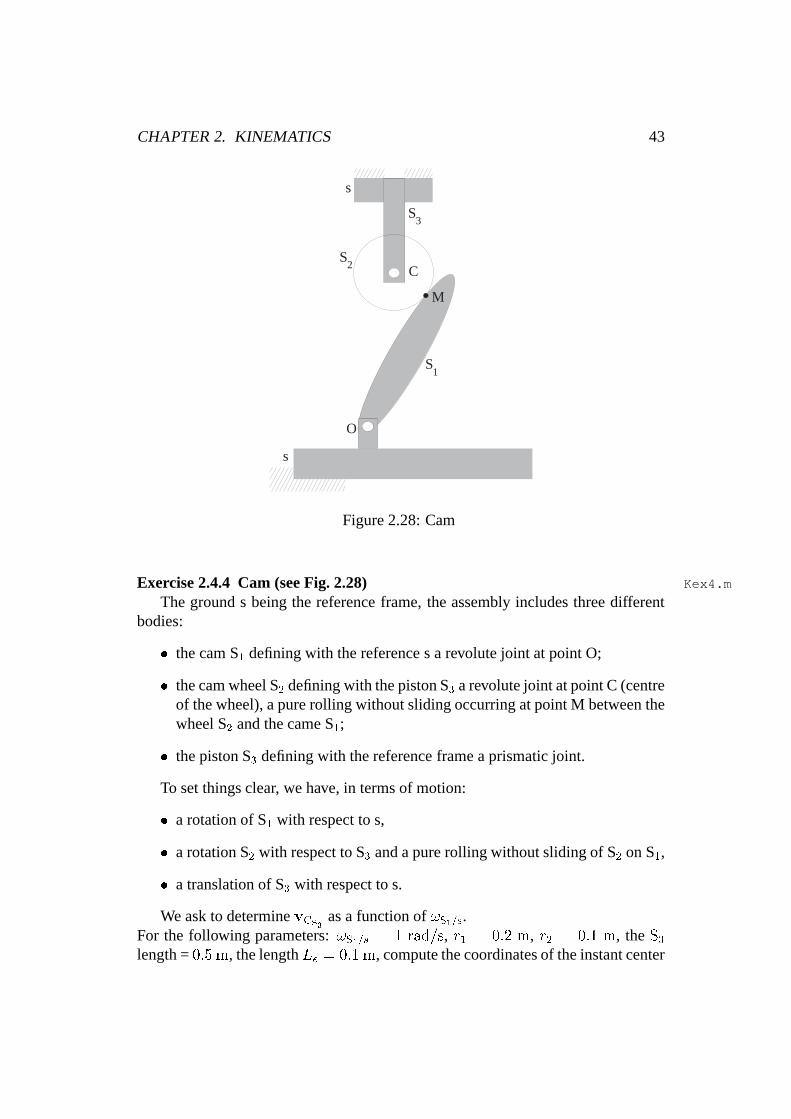
Figure 2.28: Cam
Exercise 2.4.4 Cam (see Fig. 2.28) Kex4.m
The ground s being the reference frame, the assembly includes three differentbodies:
� the cam S1 defining with the reference s a revolute joint at point O;
� the cam wheel S2 defining with the piston S3 a revolute joint at point C (centreof the wheel), a pure rolling without sliding occurring at point M between thewheel S2 and the came S1;
� the piston S3 defining with the reference frame a prismatic joint.
To set things clear, we have, in terms of motion:
� a rotation of S1 with respect to s,
� a rotation S2 with respect to S3 and a pure rolling without sliding of S2 on S1,
� a translation of S3 with respect to s.
We ask to determinevCS3 as a function of!S1=s.For the following parameters:!S1=s = 1 rad=s, r1 = 0:2 m, r2 = 0:1 m, theS3length =0:5 m, the lengthLe = 0:1 m, compute the coordinates of the instant center
CHAPTER 2. KINEMATICS 44
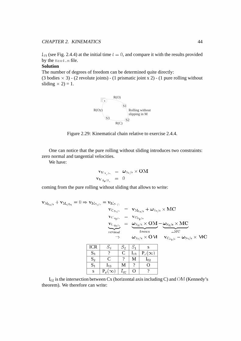
I13 (see Fig. 2.4.4) at the initial timet = 0, and compare it with the results providedby theKex4.m file.SolutionThe number of degrees of freedom can be determined quite directly:(3 bodies� 3) - (2 revolute joints) - (1 prismatic joint x 2) - (1 pure rolling withoutsliding� 2) = 1.
s
S1
S3
Rolling withoutslipping in M
R(C)
R(O)
S2
R(Oy)
Figure 2.29: Kinematical chain relative to exercise 2.4.4.
One can notice that the pure rolling without sliding introduces two constraints:zero normal and tangential velocities.
We have:
vMS1=s= !S1=s �OM
vMS2=S1= 0
coming from the pure rolling without sliding that allows to write:
vMS2=s+ vMs=S1
= 0) vMS2=s= vMS1=s
vCS2=s = vMS2=s+ !S2=s �MC
vCS3=s = vCS2=s
vCS3=s| {z }vertical
= !S1=s �OM| {z }known
+!S2=s �MC| {z }?MC
) !S1=s �OM = vCS3=s � !S2=s �MC
ICR S3 S2 S1 sS3 ? C I13 Px(1)S2 C ? M I02S1 I13 M ? Os Px(1) I02 O ?
I02 is the intersection between Cx (horizontal axis including C) andOM (Kennedy’stheorem). We therefore can write:
CHAPTER 2. KINEMATICS 45
s
s
C
O
M
S
I
I
S
S
3
02
13
2
1
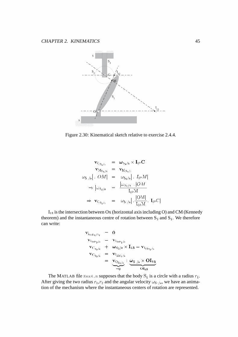
Figure 2.30: Kinematical sketch relative to exercise 2.4.4.
���vCS2=s��� = !S2=s � I02C
vMS1=s= vMS2=s��!S1=s�� : jOM j =
��!S2=s�� : jI02M j
) ��!S2=s�� =
��!S1=s�� : jOM jjI02Mj
)���vCS2=s��� =
��!S1=s�� : jOMjjI02Mj : jI02Cj
I13 is the intersection between Ox (horizontal axis including O) and CM (Kennedytheorem) and the instantaneous centre of rotation between S3 and S1. We thereforecan write:
vI13S3=S1 = 0
vI13S3=s = vI13S1=s
vCS3=s + !S3=s � I13 = vI13S1=s
vCS3=s = vI13S1=s
= vOS1=s| {z }=0
+!S1=s �OI13| {z }?OI13
The MATLAB file Kex4.m supposes that the bodyS1 is a circle with a radiusr1.After giving the two radiusr1,r2 and the angular velocity!S1=s, we have an anima-tion of the mechanism where the instantaneous centers of rotation are represented.

CHAPTER 2. KINEMATICS 46
Figure 2.31: Animation of the system of cam.
Exercise 2.4.5 Assembly of 3 bodies (see Fig. 2.32) Kex5.m
Figure 2.32: Assembly of bodies
The ground s being the reference frame, the assembly includes three differentbodies:
� a solid rod OA (lengthL) defining with the reference s a revolute joint at pointO;
� a wheel S (centre C; radiusR) defining with the solid rod AB a revolutejoint at point B (BC =R), a pure rolling without sliding occuring at point P
CHAPTER 2. KINEMATICS 47
between the wheel S and the ground s;
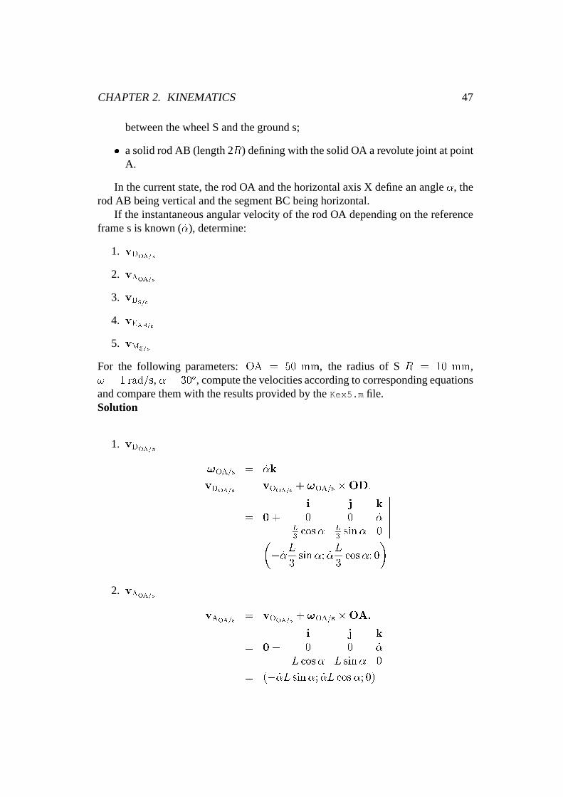
� a solid rod AB (length 2R) defining with the solid OA a revolute joint at pointA.
In the current state, the rod OA and the horizontal axis X define an angle�, therod AB being vertical and the segment BC being horizontal.
If the instantaneous angular velocity of the rod OA depending on the referenceframe s is known (_�), determine:
1. vDOA=s
2. vAOA=s
3. vBS=s
4. vEAB=s
5. vMS=s
For the following parameters:OA = 50 mm, the radius of SR = 10 mm,! = 1 rad=s,� = 30o, compute the velocities according to corresponding equationsand compare them with the results provided by theKex5.m file.Solution
1. vDOA=s
!OA=s = _�k
vDOA=s = vOOA=s + !OA=s �OD:
= 0+
������i j k
0 0 _�L3cos� L
3sin� 0
������=
�� _�
L
3sin�; _�
L
3cos�; 0
�
2. vAOA=s
vAOA=s = vOOA=s + !OA=s �OA:
= 0+
������i j k
0 0 _�L cos� L sin� 0
������= (� _�L sin�; _�L cos�; 0)
CHAPTER 2. KINEMATICS 48
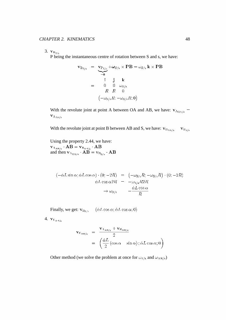
3. vBS=sP being the instantaneous centre of rotation between S and s, we have:
vBS=s = vPS=s|{z}=0
+!S=s �PB = !S=s k�PB
=
������i j k
0 0 !S=s�R R 0
������=
��!S=sR;�!S=sR; 0�With the revolute joint at point A between OA and AB, we have:vAOA=s =vAAB=s
With the revolute joint at point B between AB and S, we have:vBAB=s = vBS=s
Using the property 2.44, we have:vAAB=s �AB = vBAB=s �ABand thenvAOA=s �AB = vBS=s �AB
(� _�L sin�; _�L cos�) � (0;�2R) =��!S=sR;�!S=sR� � (0;�2R)
_�L cos�2R = �!S=sR2R! !S=s = � _�L cos�
R
Finally, we get:vBS=s = ( _�L cos�; _�L cos�; 0)
4. vEAB=s
vEAB=s =vAAB=s + vBAB=s
2
=
�_�L
2(cos�� sin�) ; _�L cos�; 0
�
Other method (we solve the problem at once for!S=s and!AB=s)
CHAPTER 2. KINEMATICS 49
vBS=s = vBAB=s = vAAB=s + !AB=sk�AB
��!S=sR;�!S=sR; 0� = (� _�L sin�; _�L cos�; 0) +
������i j k
0 0 !AB=s0 �2R 0
������=
�� _�L sin� + !AB=s2R; _�L cos�; 0�
Projection along the X axis:_�L cos� = � _�L sin� + !AB=s2R.Projection along the Y axis:�!S=sR = _�L cos� ! !S=s = � _�L cos�
R!
!AB=s =_�L2R
(cos� + sin�).
vEAB=s = vAAB=s + !AB=sk�AE
= (� _�L sin�; _�L cos�; 0) +������i j k
0 0 _�L2R
(cos�+ sin�)0 �R 0
������=
�_�L
2(cos�� sin�) ; _�L cos�; 0
�
5. vMS=s
vMS=s= vPS=s|{z}
=0
+!S=s �PM = !S=sk�PM
= 0+
������i j k
0 0 � _�L cos�R
0 2R 0
������= (2 _�L cos�; 0)
The file Kex5.m illustrates the exercise. First, the geometrical parameters of thesystem (R, d, L, p), and the angular velocity of S1 have to be introduced. Then, thefive velocitiesvDOA=s, vAOA=s, vBS=s, vEAB=s, vMS=s
are calculated.
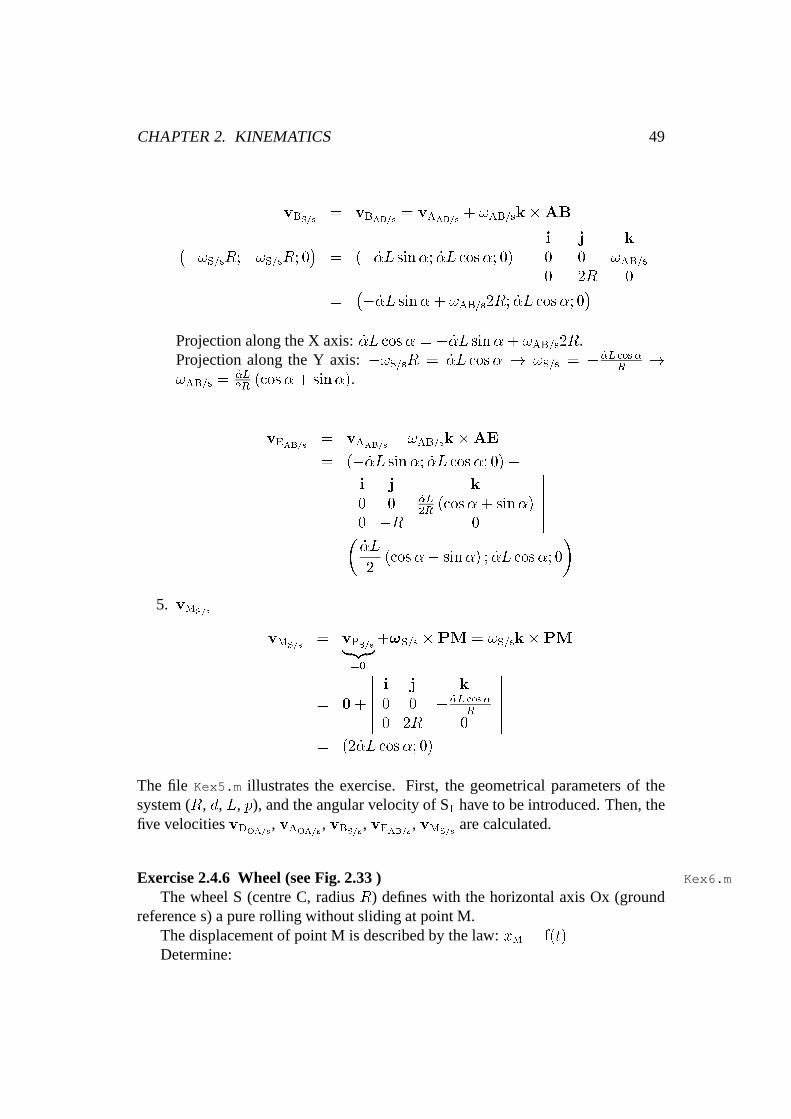
Exercise 2.4.6 Wheel (see Fig. 2.33 ) Kex6.m
The wheel S (centre C, radiusR) defines with the horizontal axis Ox (groundreference s) a pure rolling without sliding at point M.
The displacement of point M is described by the law:xM = f(t)Determine:
CHAPTER 2. KINEMATICS 50
xxxxxxxxxxxxxxxxxxxxxxxxxxxxxxxxxxxxxxxxxxxxxxxxxxxxxxxxxxxxxxxxxxxxxxxxxxxxxxxxxxxxxxxxxxxxxxxxxxxxxxxxxxxxxxxxxxxxxxxxxxxxxxxxxxxxxxxxxxxxxxxxxxxxxxxxxxxxxxxxxxxxxxxxxxxxxxxxxxxxxxxxxxxxxxxxxxxxxxxxxxxxxxxxxxxxxxxxxxxxxxxx
y
x
+
xxxx
xxxx
S
s
R C
MO
Figure 2.33: Wheel
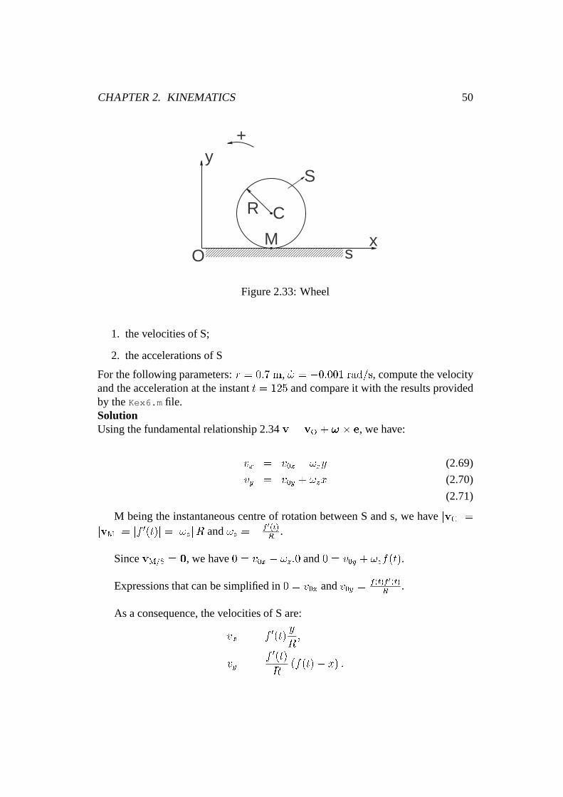
1. the velocities of S;
2. the accelerations of S
For the following parameters:r = 0:7 m, _! = �0:001 rad=s, compute the velocityand the acceleration at the instantt = 125 and compare it with the results providedby theKex6.m file.SolutionUsing the fundamental relationship 2.34v = vO + ! � e, we have:
vx = v0x � !zy (2.69)
vy = v0y + !zx (2.70)
(2.71)
M being the instantaneous centre of rotation between S and s, we havejvCj =jvMj = jf 0(t)j = j!zjR and!z = �f 0(t)
R.
SincevM=S = 0, we have0 = v0x � !z:0 and0 = v0y + !zf(t).
Expressions that can be simplified in0 = v0x andv0y =f(t)f 0(t)
R.
As a consequence, the velocities of S are:
vx = f 0(t)y
R;
vy =f 0(t)R
(f(t)� x) :

CHAPTER 2. KINEMATICS 51
Coming from these, the accelerations are:
ax =v0xdt� !z
dty � !zv0y � !2zx; (2.72)
ay =v0ydt
+!zdtx� !zv0x � !2zy; (2.73)
ax =f 00(t)R
y +f 0(t)R
f(t)f 0(t)R
� f 02(t)R2
x; (2.74)
ay =f 02(t) + f(t)f 00(t)
R� f 00(t)
Rx� f 02(t)
R2y; (2.75)
ax =f 02(t)R2
f � f 02(t)R2
x +f 00(t)R
y; (2.76)
ay =f 02 + ff 00
R� f 00
Rx� f 02
R2y: (2.77)
The file Kex6.m illustrates this exercise by giving an animation of the wheelrolling on a fixed ground. First, the geometrical parameters of the system (r, !)have to be introduced. Then, the user need to choose between a representation ofthe velocity vector or the acceleration vector during the wheel motion. We supposein this exercise that, the angular acceleration of the body S is constant.
Figure 2.34: In the animation given by the Kex6.m file we have either the velocityvector or the acceleration vector of a point of the circle.
Exercise 2.4.7 Ship motion (see Fig. 2.35) Kex7.m
A sailing O ship purely moves forward along its longitudinal axis (this axis canbe seen as the intersection between the longitudinal symmetry plane of the ship andthe surface of the sea). For such a motion to occur, the wind w should blow in thebackward face of the sail.
If � is the angle between the longitudinal axis and the wind direction and theangle between the longitudinal axis and the sail orientation (see Fig. 2.35), deter-mine the limit angle lim so that a longitudinal motion of the ship still occurs. Show
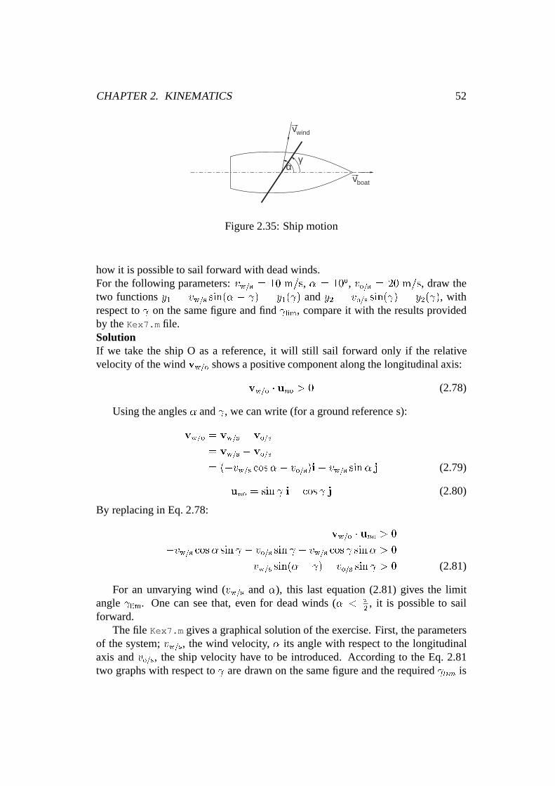
CHAPTER 2. KINEMATICS 52
γα
vwind
vboat
Figure 2.35: Ship motion
how it is possible to sail forward with dead winds.For the following parameters:vw=s = 10 m=s, � = 10o, vo=s = 20 m=s, draw thetwo functionsy1 = vw=s sin(� � ) = y1( ) andy2 = vo=s sin( ) = y2( ), withrespect to on the same figure and find lim, compare it with the results providedby theKex7.m file.SolutionIf we take the ship O as a reference, it will still sail forward only if the relativevelocity of the windvw=o shows a positive component along the longitudinal axis:
vw=o � uno > 0 (2.78)
Using the angles� and , we can write (for a ground reference s):
vw=o = vw=s � vo=s
= vw=s � vo=s
= (�vw=s cos�� vo=s)i� vw=s sin� j (2.79)
uno = sin i� cos j (2.80)
By replacing in Eq. 2.78:
vw=o � uno > 0
�vw=s cos� sin � vo=s sin + vw=s cos sin� > 0
vw=s sin(�� )� vo=s sin > 0 (2.81)
For an unvarying wind (vw=s and�), this last equation (2.81) gives the limitangle lim. One can see that, even for dead winds (� < �
2, it is possible to sail
forward.The fileKex7.m gives a graphical solution of the exercise. First, the parameters
of the system;vw=s, the wind velocity,� its angle with respect to the longitudinalaxis andvo=s, the ship velocity have to be introduced. According to the Eq. 2.81two graphs with respect to are drawn on the same figure and the required lim is
CHAPTER 2. KINEMATICS 53
α
α
vwind
boat path
Figure 2.36: Ship motion.
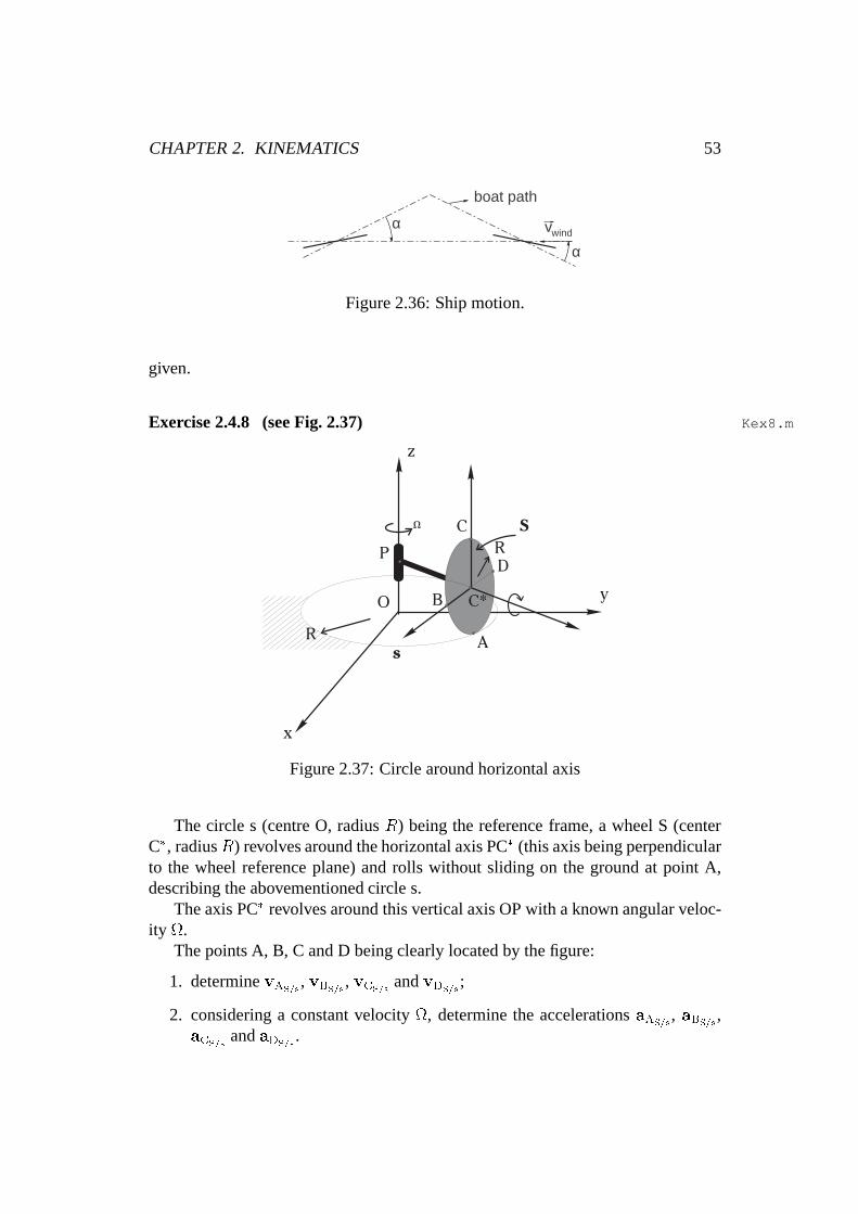
given.
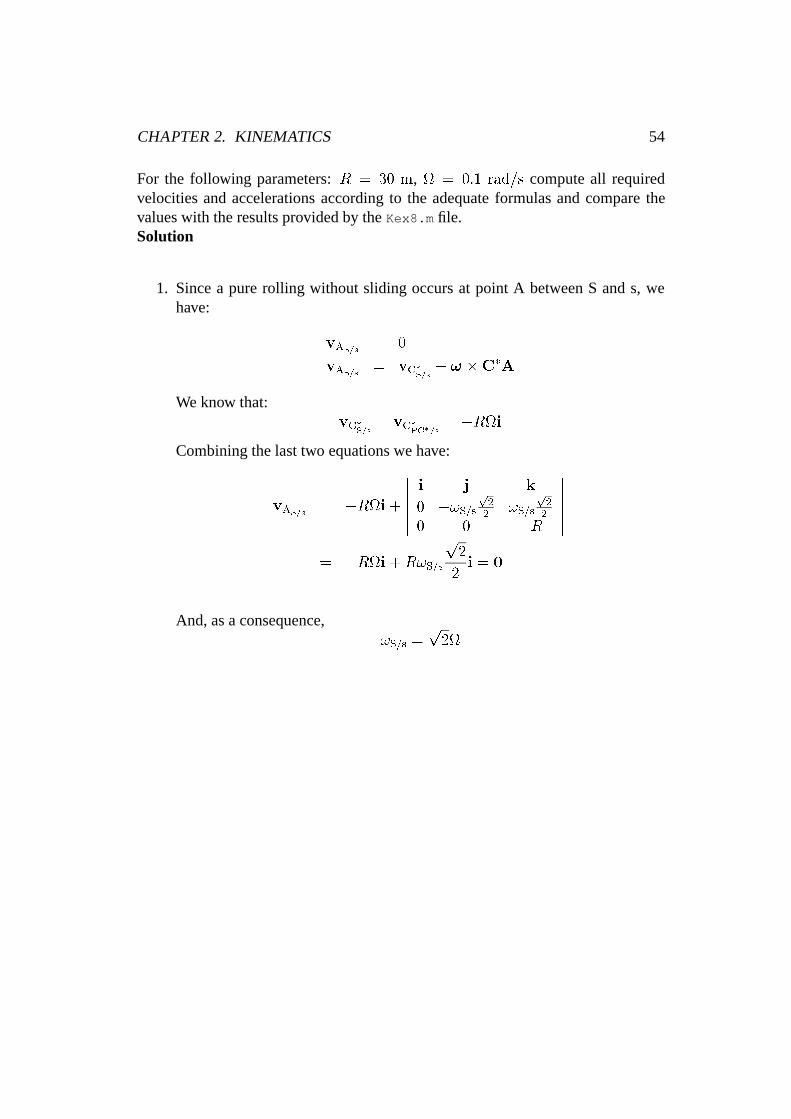
Exercise 2.4.8 (see Fig. 2.37) Kex8.m
Figure 2.37: Circle around horizontal axis
The circle s (centre O, radiusR) being the reference frame, a wheel S (centerC�, radiusR) revolves around the horizontal axis PC� (this axis being perpendicularto the wheel reference plane) and rolls without sliding on the ground at point A,describing the abovementioned circle s.
The axis PC� revolves around this vertical axis OP with a known angular veloc-ity .
The points A, B, C and D being clearly located by the figure:
1. determinevAS=s, vBS=s , vCS=s andvDS=s ;
2. considering a constant velocity, determine the accelerationsaAS=s, aBS=s ,aCS=s andaDS=s .
CHAPTER 2. KINEMATICS 54
For the following parameters:R = 30 m, = 0:1 rad=s compute all requiredvelocities and accelerations according to the adequate formulas and compare thevalues with the results provided by theKex8.m file.Solution
1. Since a pure rolling without sliding occurs at point A between S and s, wehave:
vAS=s = 0
vAS=s = vC�S=s
+ ! �C�A
We know that:vC�
S=s= vC�
PC�=s= �Ri
Combining the last two equations we have:
vAS=s = �Ri +������i j k
0 �!S=sp22
!S=sp22
0 0 �R
������= �Ri +R!S=s
p2
2i = 0
And, as a consequence,!S=s =
p2
CHAPTER 2. KINEMATICS 55
The other velocities are easily determined as shown here below:
vBS=s = vC�S=s
+ ! �C�B
= �Ri+������i j k
0 � R 0 0
������= �Ri+Rj +Rk
vCS=s = vC�S=s
+ ! �C�C
= �Ri+������i j k
0 � 0 0 R
������= �Ri� Ri = �2Ri
vDS=s = vC�S=s
+ ! �C�D
= �Ri+������
i j k
0 � �R 0 0
������= �Ri� Rj�Rk
2. Quite logically, we have:aPS=s = 0
M being a point randomly selected on S, we have:
aMS=s=
d!
dt�PM+ ! � (! �PM) ;M 2 S
We also have:
! = !S=s = p2AP
Rp2=
AP
R
If � is the instantaneous angle between PC and Ox during the motion, we canwrite:
AP = Rk�R cos�i� R sin�j
! = (k� cos�i� sin�j) :
d!
dt= (sin�i� cos�j)
d�
dt= 2 (sin�i� cos�j) :
For the current position, we have:� = �
2,
CHAPTER 2. KINEMATICS 56
! = (k� j),d!dt
= 2i,andaMS=s
= 2i�PM+ 2 ((k� j) �PM) (k� j)� 22PM.We finally get:
aAS=s = 2R (j+ k)
aBS=s = �2R (2i+ j)
aCS=s = �2R (3j+ k)
aDS=s = 2R (2i� j)
The MATLAB file Kex8.m illustrates this exercise by calculating all required ve-locities and accelerations assume toR the radius of the body S, and the angularvelocity ofPC� around the vertical axisOP, are known.
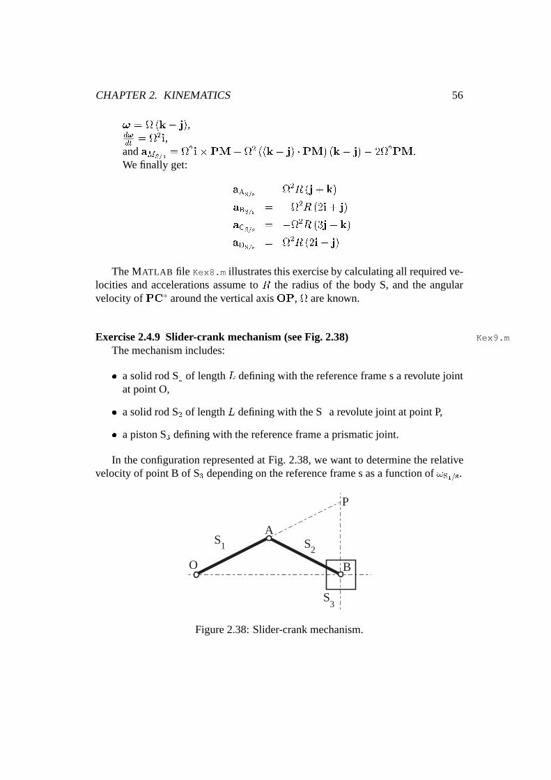
Exercise 2.4.9 Slider-crank mechanism (see Fig. 2.38) Kex9.m
The mechanism includes:
� a solid rod S1 of lengthL defining with the reference frame s a revolute jointat point O,
� a solid rod S2 of lengthL defining with the S1 a revolute joint at point P,
� a piston S3 defining with the reference frame a prismatic joint.
In the configuration represented at Fig. 2.38, we want to determine the relativevelocity of point B of S3 depending on the reference frame s as a function of!S1=s.
O
S S
S
1 2
3
A
P
B
Figure 2.38: Slider-crank mechanism.
CHAPTER 2. KINEMATICS 57
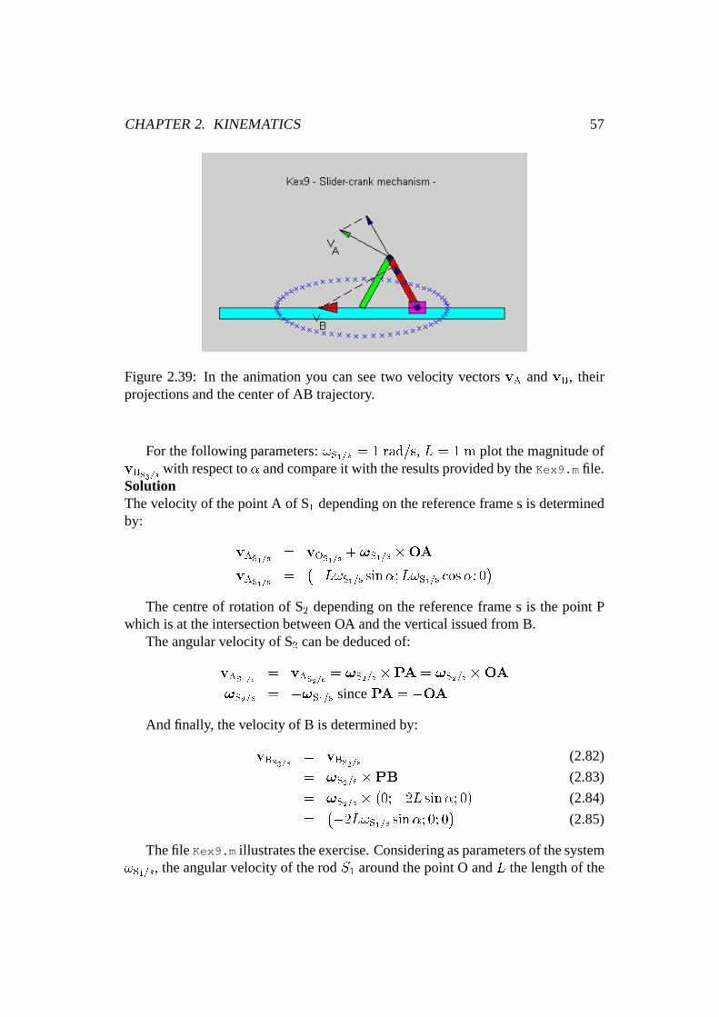
Figure 2.39: In the animation you can see two velocity vectorsvA andvB, theirprojections and the center of AB trajectory.
For the following parameters:!S1=s = 1 rad=s, L = 1 m plot the magnitude ofvBS3=s with respect to� and compare it with the results provided by theKex9.m file.SolutionThe velocity of the point A of S1 depending on the reference frame s is determinedby:
vAS1=s = vOS1=s + !S1=s �OA
vAS1=s =��L!S1=s sin�;L!S1=s cos�; 0�
The centre of rotation of S2 depending on the reference frame s is the point Pwhich is at the intersection between OA and the vertical issued from B.
The angular velocity of S2 can be deduced of:
vAS1=s = vAS2=s = !S2=s �PA = !S2=s �OA
!S2=s = �!S1=s sincePA = �OA
And finally, the velocity of B is determined by:
vBS3=s = vBS2=s (2.82)
= !S2=s �PB (2.83)
= !S2=s � (0;�2L sin�; 0) (2.84)
=��2L!S1=s sin�; 0; 0� (2.85)
The fileKex9.m illustrates the exercise. Considering as parameters of the system!S1=s, the angular velocity of the rodS1 around the point O andL the length of the
CHAPTER 2. KINEMATICS 58
two rods S1 andS2 have been introduced, the velocities of the points A and B arecalculated. An animation of the mechanism is performed (see Fig. 2.39). The me-chanical system is shown in different configurations when the solid S1 turns aroundthe Oz axis. The two velocity vectors and their projection on the AB axis are rep-resented. Thus the user can see that the relation of equiprojectivity (see Eq. 2.44) isalways verified.
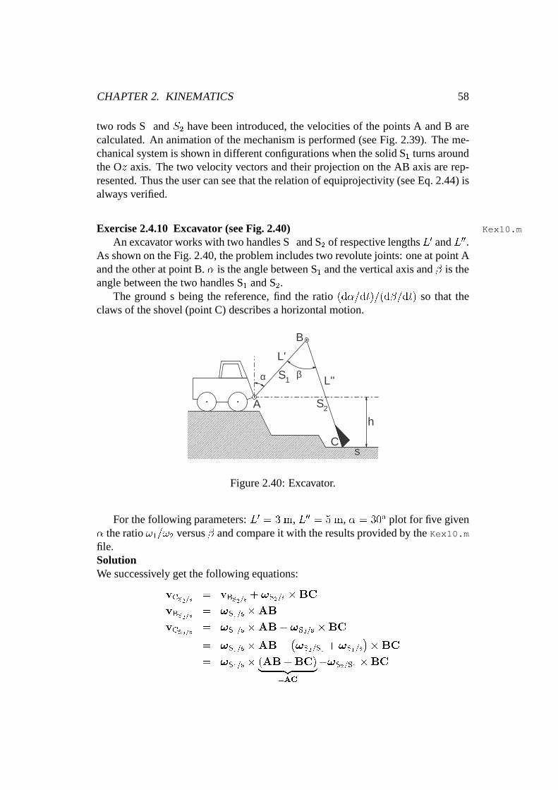
Exercise 2.4.10 Excavator (see Fig. 2.40) Kex10.m
An excavator works with two handles S1 and S2 of respective lengthsL0 andL00.As shown on the Fig. 2.40, the problem includes two revolute joints: one at point Aand the other at point B.� is the angle between S1 and the vertical axis and� is theangle between the two handles S1 and S2.
The ground s being the reference, find the ratio(d�=dt)=(d�=dt) so that theclaws of the shovel (point C) describes a horizontal motion.
xxxxxxxxxxxxxxxxxxxxxxxxxxxxxxxxxxxxxxxxxxxxxxxxxxxxxxxxxxxxxxxxxxxxxxxxxxxxxxxxxxxxxxxxxxxxxxxxxxxxxxxxxxxxxxxxxxxxxxxxxxxxxxxxxxxxxxxxxxxxxxxxxxxxxxxxxxxxxxxxxxxxxxxxxxxxxxxxxxxxxxxxxxxxxxxxxxxxxxxxxxxxxxxxxxxxxxxxxxxxxxxxxxxxxxxxxxxxxxxxxxxxxxxxxxxxxxxxxxxxxxxxxxxxxxxxxxxxxxxxxxxxxxxxxxxxxxxxxxxxxxxxxxxxxxxxxxxxxxxxxxxxxxxxxxxxxxxxxxxxxxxxxxxxxxxxxxxxxxxxxxxxxxxxxxxxxxxxxxxxxxxxxxxxxxxxxxxxxxxxxxxxxxxxxxxxxxxxxxxxxxxxxxxxxxxxxxxxxxxxxxxxxxxxxxxxxxxxxxxxxxxxxxxxxxxxxxxxxxxxxxxxxxxxxxxxxxxxxxxxxxxxxxxxxxxxxxxxxxxxxxxxxxxxxxxxxxxxxxxxxxxxxxxxxxxxxxxxxxxxxxxxxxxxxxxxxxxxxxxxxxxxxxxxxxxxxxxxxxxxxxxxxxxxxxxxxxxxxxxxxxxxxxxxxxxxxxxxxxxxxxxxxxxxxxxxxxxxxxxxxxxxxxxxxxxxxxxxxxxxxxxxxxxxxxxxxxxxxxxxxxxxxxxxxxxxxxxxxxxxxxxxxxxxxxxxxxxxxxxxxxxxxxxxxxxxxxxxxxxxxxxxxxxxxxxxxxxxxxxxxxxxxxxxxxxxxxxxxxxxxxxxxxxxxxxxxxxxxxxxxxxxxxxxxxxxxxxxxxxxxxxxxxxxxxxxxxxxxxxxxxxxxxxxxxxxxxxxxxxxxxxxxxxxxxxxxxxxxxxxxxxxxxxxxxxxxxxxxxxxxxxxxxxxxxxxxxxxxxxxxxxxxxxxxxxxxxxxxxxxxxxxxxxxxxxxxxxxxxxxxxxxxxxxxxxxxxxxxxxxxxxxxxxxxxxxxxxxxxxxxxxxxxxxxxxxxxxxxxxxxxxxxxxxxxxxxxxxxxxxxxxxxxxxxxxxxxxxxxxxxxxxxxxxxxxxxxxxxxxxxxxxxxxxxxxxxxxxxxxxxxxxxxxxxxxxxxxxxxxxxxxxxxxxxxxxxxxxxxxxxxxxxxxxxxxxxxxxxxxxxxxxxxxxxxxxxxxxxxxxxxxxxxxxxxxxxxxxxxxxxxxxxxxxxxxxxxxxxxxxxxxxxxxxxxxxxxxxxxxxxxxxxxxxxxxxxxxxxxxxxxxxxxxxxxxxxxxxxxxxxxxxxxxxxxxxxxxxxxxxxxxxxxxxxxxxxxxxxxxxxxxxxxxxxxxxxxxxxxxxxxxxxxxxxxxxxxxxxxxxxxxxxxxxxxxxxxxxxxxxxxxxxxxxxxxxxxxxxxxxxxxxxxxxxxxxxxxxxxxxxxxxxxxxxxxxxxxxxxxxxxxxxxxxxxxxxxxxxxxxxxxxxxxxxxxxxxxxxxxxxxxxxxxxxxxxxxxxxxxxxxxxxxxxxxxxxxxxxxxxxxxxxxxxxxxxxxxxxxxxxxxxxxxxxxxxxxxxxxxxxxxxxxxxxxxxxxxxxxxxxxxxxxxxxxxxxxxxxxxxxxxxxxxxxxxxxxxxxxxxxxxxxxxxxxxxxxxxxxxxxxxxxxxxxxxxxxxxxxxxxxxxxxxxxxxxxxxxxxxxxxxxxxxxxxxxxxxxxxxxxxxxxxxxxxxxxxxxxxxxxxxxxxxxxxxxxxxxxxxxxxxxxxxxxxxxxxxxxxxxxxxxxxxxxxxxxxxxxxxxxxxxxxxxxxxxxxxxxxxxxxxxxxxxxxxxxxxxxxxxxxxxxxxxxxxxxxxxxxxxxxxxxxxxxxxxxxxxxxxxxxxxxxxxxxxxxxxxxxxxxxxxxxxxxxxxxxxxxxxxxxxxxxxxxxxxxxxxxxxxxxxxxxxxxxxxxxxxxxxxxxxxxxxxxxxxxxxxxxxxxxxxxxxxxxxxxxxxxxxxxxxxxxxxxxxxxxxxxxxxxxxxxxxxxxxxxxxxxxxxxxxxxxxxxxxxxxxxxxxxxxxxxxxxxxxxxxxxxxxxxxxxxxxxxxxxxxxxxxxxxxxxxxxxxxxxxxxxxxxxxxxxxxxxxxxxxxxxxxxxxxxxxxxxxxxxxxxxxxxxxxxxxxxxxxxxxxxxxxxxxxxxxxxxxxxxxxxxxxxxxxxxxxxxxxxxxxxxxxxxxxxxxxxxxxxxxxxxxxxxxxxxxxxxxxxxxxxxxxxxxxxxxxxxxxxxxxxxxxxxxxxxxxxxxxxxxxxxxxxxxxxxxxxxxxxxxxxxxxxxxxxxxxxxxxxxxxxxxxxxxxxxxxxxxxxxxxxxxxxxxxxxxxxxxxxxxxxxxxxxxxxxxxxxxxxxxxxxxxxxxxxxxxxxxxxxxxxxxxxxxxxxxxxxxxxxxxxxxxxxxxxxxxxxxxxxxxxxxxxxxxxxxxxxxxxxxxxxxxxxxxxxxxxxxxxxxxxxxxxxxxxxxxxxxxxxxxxxxxxxxxxxxxxxxxxxxxxxxxxxxxxxxxxxxxxxxxxxxxxxxxxxxxxxxxxxxxxxxxxxxxxxxxxxxxxxxxxxxxxxxxxxxxxxxxxxxxxxxxxxxxxxxxxxxxxxxxxxxxxxxxxxxxxxxxxxxxxxxxxxxxxxxxxxxxxxxxxxxxxxxxxxxxxxxxxxxxxxxxxxxxxxxxxxxxxxxxxxxxxxxxxxxxxxxxxxxxxxxxxxxxxxxxxxxxxxxxxxxxxxxxxxxxxxxxxxxxxxxxxxxxxxxxxxxxxxxxxxxxxxxxxxxxxxxxxxxxxxxxxxxxxxxxxxxxxxxxxxxxxxxxxxxxxxxxxxxxxxxxxxxxxxxxxxxxxxxxxxxxxxxxxxxxxxx
α β
A
B
C
h
L''
L'
s
S2
S1
Figure 2.40: Excavator.
For the following parameters:L0 = 3 m, L00 = 5 m, � = 30o plot for five given� the ratio!1=!2 versus� and compare it with the results provided by theKex10.m
file.SolutionWe successively get the following equations:
vCS2=s = vBS2=s + !S2=s �BC
vBS2=s = !S1=s �AB
vCS2=s = !S1=s �AB+ !S2=s �BC
= !S1=s �AB+�!S2=S1 + !S1=s
��BC
= !S1=s � (AB+BC)| {z }=AC
+!S2=S1 �BC
BIBLIOGRAPHY 59
AC = [L0 sin� + L00 sin (� � �)] i+ [L0 cos�� L00 cos (� � �)] j
BC = [�L00 sin (� � �)] i+ [�L00 cos (� � �)] j
!S1=s �AC =
������i j k
0 0 !1L0 sin� + L00 sin (� � �) L0 cos�� L00 cos (� � �) 0
������= �!1 [L0 cos�� L00 cos (� � �)] i+ !1 [L
0 sin� + L00 sin (� � �)] j
!S2=S1 �BC =
������i j k
0 0 !2�L00 sin (� � �) �L00 cos (� � �) 0
������= !2L
00 cos (� � �) i� !2L00 sin (� � �) j
Still vCS2=s has to be parallel to the horizontal axisi, we can write:
!2:L00 sin (� � �) = !1 [L
0 sin�+ L00 sin (� � �)]
!2!1
=[L0 sin� + L00 sin (� � �)]
L00 sin (� � �)d�dtd�dt
=!1!2
=1
1 + L0 sin�L00 sin(���)
The file Kex10.m gives a graphical solution of the exercise. The parameters ofthe system areL0, the length of the bodyS1, L00, the length of the bodyS2. We plotfor five given� the ratio!1=!2 with respect to�.
Bibliography
[1] J.W. McNabb B.B. Muvdi, A.W. Al-Khafaji. Dynamics For Engineers.Springer-Verlag, New York, 1997.
[2] Serge Boucher.Mécanique Rationnelle. Editions des étudiants de la FacultéPolytechnique de Mons, Mons, Belgium, 1999. (in French, 7 volumes).
[3] E.Russel Johnston JR Ferdinand P. Beer.Vector Mechanics For engineers. Stat-ics and Dynamics. McGraw-Hill, USA, 1997.
[4] J.J. Uicker J.E. Shigley.Theory of Machines and Mechanics.McGraw-Hill,New York, 1995.
[5] Irving H. Shames. Engineering Mechanics. Statics and Dynamics. PrenticeHall, Upper Saddle River, New Jersey, USA, 1996.
BIBLIOGRAPHY 60
[6] Kenneth J. Waldron and Gary L. Kinzel.Kinematics, Dynamics and Design ofMachinery. John Wiley and Sons, New York, 1999.