Chapter 2

KINETIC THEORY

2.1 Distribution Functions

A plasma is an ensemble of particles electrons e, ions i and neutrals n withdifferent positions r and velocities v which move under the influence of externalforces (electromagnetic fields, gravity) and internal collision processes (ionization,Coulomb, charge exchange etc.)

However, what we observe is some “average” macroscopic plasma parameterssuch as j - current density, ne - electron density, P - pressure, Ti - ion temperatureetc.

These parameters are macrsocopic averages over the distribution of particlevelocities and/or positions.

In this lecture we

• Introduce the concept of the distribution function fα(r, v, t) for a givenplasma species;

• Derive the force balance equation (Boltzmann equation) that drives thetemporal evolution of fα(r, v, t);

• Show that low order velocity moments of fα(r, v, t) give various importantmacroscopic parameters;

• Consider the role of collision processes in coupling the charged and neutralspeicies dynamics in a plasma and

• Show that low order velocity moments of the Boltzmann equation give“fluid” equations for the evolution of the macroscopic quantities.

30

2.2 Phase Space

Consider a single particle of species α. It can be described by a position vector

r = xi + yj + zk

in configuration space and a velocity vector

v = vxi + vy j + vzk

in velocity space. The coordinates (r, v) define the particle position in phasespace.

For multi-particle systems, we introduce the distribution function fα(r, v, t)for species α defined such that

fα(r, v, t) dr dv = dN(r, v, t) (2.1)

is the number of particles in the element of volume dV = dv dr in phase space.Here, dr ≡ d3r ≡ dxdydz and dv ≡ d3v ≡ dvxdvydvz fα(r, v, t) is a positivefinite function that decreases to zero as |v | becomes large.

y

x

z

rdx

dy

dz

v

v

v

v

dv

x

y

z

z

dvx

dvy

o o

Figure 2.1: Left: A configuration space volume element dr = dxdydz at spatial

position r. Right: The equivalent velocity space element. Together these two

elements constitute a volume element dV = drdv at position (r, v) in phase

space.

The element dr must not be so small that it doesn’t contain a statisticallysignificant number of particles. This allows fα(r, v, t) to be approximated by

2.3 The Boltzmann Equation 31

a continuous function. For example, for typical densities in H-1NF 1012 m−3,dr ≈ 10−12 m−3 =⇒ dr

∫fα(r, v, t) dv ∼ 106 particles.

Some defnitions:

• If fα depends on r, the distribution is inhomogeneous

• If fα is independent of r, the distribution is homogeneous

• If fα depends on the direction of v, the distribution is anisotropic

• If fα is independent of the direction of v, the distribution is isotropic

• A plasma in thermal equilibrium is characterized by a homogeneous, isotropicand time-independent distribution function

2.3 The Boltzmann Equation

As we have seen, the distribution of particles is a function of both time andthe phase space coordinates (r, v). The Boltzmann equation describes the timeevolution of f under the action of external forces and internal collisions. Theremainder of this section draws on the derivation given in [2].

fα(r, v, t) changes because of the flux of particles across the surface boundingthe elemental volume drdv in phase space. This can arise continuously due toparticle velocity and external forces (accelerations) or discontinuously throughcollisions. The collisional contribution to the rate of change ∂f/∂t of the distri-bution function is written as (∂f/∂t)coll.

To account for continuous phase space flow we use the divergence theorem∫S

E.ds =∫∆V

∇.E dV (2.2)

applied to the six dimensional phase space surface S bounding the phase spacevolume ∆V enclosing the six dimensional vector field E.

Now note that conservation of particles requires that the rate of particle flowover the surface ds bounding the element ∆V plus those generated by collisionsbe equal to the rate at which particle phase space density changes with time.If we let V = (v, a) be the generalized “velocity” vector for our mathematicalphase space (r, v), then the rate of flow over S into the volume element is

−∫

Sds. [V f ]

Compare V f with the definition of particle flux Γ(r, t) - a configuration spacequantity [Eq. (2.14)]. Using the divergence theorem, this contribution can bewritten

−∫∆V

drdv [∇r.(vf) + ∇v.(af)]

32

where ∇r. is the divergence with respect to r and ∇v. is the divergence operatorwith respect to v. For example

∇r. ≡ i∂

∂x+ j

∂

∂y+ k

∂

∂z

Since ∆V is an elemental volume, the integrand changes negligibly and canbe removed from the integral. The inclusion of the continuous phase space flowterm and the discontinuous collision term then gives the result

∂f

∂t= −∇r.(vf) − ∇v.(af) +

(∂f

∂t

)coll

. (2.3)

The acceleration can be written in terms of the force F = ma applied or actingon the particle species. For plasmas, the dominant force is electromagnetic, theLorentz force

F = q(E + v×B) ≡ ma. (2.4)

Using the vector identity (product rule)

∇.(fV ) = ∇f .V + f∇.V

we can write∇v.(v×B)f = (v×B).∇vf (why?)

Moreover, since r and v are independent coordinates, we finally obtain the Boltz-mann equation

∂f

∂t+ v.∇rf +

q

m(E + v×B).∇vf =

(∂f

∂t

)coll

(2.5)

Since f is a function of seven variables r, v, t its total derivative with respectto time is

df

dt=

∂f

∂t

+∂f

∂x

dx

dt+

∂f

∂y

dy

dt+

∂f

∂z

dz

dt

+∂f

∂vx

dvx

dt+

∂f

∂vy

dvy

dt+

∂f

∂vz

dvz

dt(2.6)

The second line is just the expansion of the term v.∇rf and the third, the terma.∇vf . Thus Eq. (2.3) is simply saying that df/dt = 0 unless there are collisions!When there are no collisions, (∂f/∂t)coll = 0 and Eq. (2.5) is called the Vlasovequation.

The quantity df/dt is called the convective derivative. It contains terms dueto the explicit variation of f (or any other configuration or phase space quantity)

2.3 The Boltzmann Equation 33

with time (∂f/∂t) and an additional term v.∇f that accounts for variations inf due to the change in location in time (convection) of f to a position where fhas a different value. As an example, consider water flow at the outlet of a tap.The water is moving, but the flow pattern is not changing explicitly with time(∂f/∂t) = 0. However, the velocity of a fluid element changes on leaving the tapdue to, for example, the force of gravity. The flow velocity changes in time as thewater falls because the term (v.∇)v is nonzero. When the tap is turned off, theflow slows and stops due to (∂f/∂t) �= 0.

What does df/dt = 0 mean? With reference to Fig 2.2, consider a group ofparticles at point A with 2-D phase space density f(x, v). As time passes, theparticles will move to B as a result of their velocity at A and their velocity willchange as a result of forces acting. Since F = F (x, v), all particles at A will beaccelerated the same amount. Since the particles move together, the density atB will be the same as at A, f can only be changed by collisions.

It is important to understand that x and v are independent variables or co-ordinates, even though v = dx/dt for a given particle. The reason is that theparticle velocity is not a function of position - it can have any velocity at anyposiiton.

Collisions

A

B

x

dx

vx

dvx

Collisions

Figure 2.2: Evolution of phase space volume element under collisions

34

2.4 Plasma Macroscopic Variables

Macroscopic variables (measurable quantities) are obtained by taking appropriatevelocity moments of the distribution function. It is perhaps not surprising that thedynamical evolution of these quantities can be described by equations obtainedby taking the corresponding velocity moments of the Boltzmann equation. Theseequations (the fluid equations) are derived later in this chapter. For simplicity,and where possible, we drop the α subscript denoting the particle species for theremainder of this analysis.

2.4.1 Number density

Integration over all velocities gives the particle number density

nα =∫

fα(r, v, t) dv (2.7)

This is the zeroth order velocity moment.Multiply by mass or charge to obtain

mass density : ραm = mα

∫fα(r, v, t) dv (2.8)

charge density : ραq = qα

∫fα(r, v, t) dv (2.9)

2.4.2 Taking averages using the distribution function

The quantity

f(r, v, t) =f(r, v, t)∫f(r, v, t)dv

=f(r, v, t)

n(r, t)(2.10)

is the probability of finding one particle in a unit volume of ordinary (configura-tion) space centred at r and in a unit volume of velocity space centred at v attime t. The distribution average of some quantity g(r, v, t) is then the value of gat (r, v, t) times the probability that there is a particle with these coodinates

g(r, t) =∫

dv g(r, v, t) f(r, v, t) (2.11)

or

g(r, t) =1

n(r, t)

∫dv g(r, v, t) f(r, v, t) (2.12)

2.4.3 First velocity moment

The average velocity is obtained from the first velocity moment of f .

v(r, t) =1

n(r, t)

∫dv v f(r, v, t) (2.13)

2.4 Plasma Macroscopic Variables 35

Note that v(r, t) can be a function of r and t though v (a coordinate) is not.This is because f varies with r and t.

Multiplying the average velocity by the particle number density gives theparticle flux

Γ = nv =∫

dv v f(r, v, t) (2.14)

In a similar fashion, multiplying the flux by the charge density gives the chargeflux density or current density for a given species

j = qnv = qΓ (2.15)

2.4.4 Second velocity moment

Taking the second central moment with respect to average velocity v gives thepressure tensor (or kinetic stress tensor)

↔P (r, t) = m

∫dv (v − v)(v − v) f(r, v, t) (2.16)

We define vr = v − v, the random thermal velocity of the particles where v isthe mean drift velocity. Then vrvr is the tensor or dyadic

vrvr =

vxvx vxvy vxvz

vyvx vyvy vyvz

vzvx vzvy vzvz

(2.17)

and clearly (vrvr)αβ = (vrvr)βα so that↔P has only six independent components

which we write as

Pαβ = m∫

dv vrαvrβ f(r, v, t)

= mnvrαvrβ (2.18)

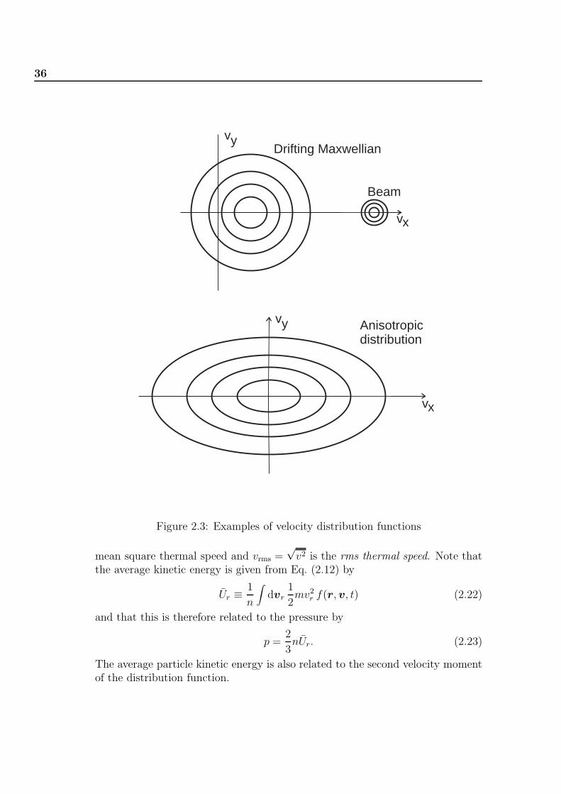
Now consider the distribution function f to be isotropic in the system driftingwith velocity v(r, t) (see Fig 2.3). Because f is isotropic in this system, vr = 0and

vrαvrβ = 0 α �= β (2.19)

= v2rα = v2

rβ = v2r/3 (2.20)

(show this result) and↔P→ p = nmv2

r/3. (2.21)

p is the rate of transfer of particle momentum in any direction. It has dimensionsforce/area or pressure. v2

r (or simply v2 when the plasma is not drifting) is the

36

vy

Beam

Drifting Maxwellianvy

vx

vx

Anisotropicdistribution

Figure 2.3: Examples of velocity distribution functions

mean square thermal speed and vrms =√

v2 is the rms thermal speed. Note thatthe average kinetic energy is given from Eq. (2.12) by

Ur ≡ 1

n

∫dvr

1

2mv2

r f(r, v, t) (2.22)

and that this is therefore related to the pressure by

p =2

3nUr. (2.23)

The average particle kinetic energy is also related to the second velocity momentof the distribution function.

2.5 Maxwell-Boltzmann Distribution 37

2.5 Maxwell-Boltzmann Distribution

So far we have shown how low order velocity moments of the particle distri-bution function are related to macroscopic parameters such as current density,pressure etc. without looking at the details of the distribution function itself. Aparticularly important velocity distribution function is the Maxwell-Boltzmanndistribution, or Maxwellian. It describes the spread of velocities for a gas whichis in thermal equilibrium. Such a system can be described by a simple Gaussianspread of velocities, the half-width being related to the gas temperature. As al-ways, the zeroth moment of such a distribution is the particle number density.Because a Gaussian has even symmetry, the odd moment will vanish unless thedistribution happens to be drifting with respect to the laboratory frame. Thesecond velocity moment is related to the temperature and also, not surprisingly,reveals a link between the gas pressure and temperature. In this section, we intro-duce this important distribution and its variants and discuss some of its physicalramifications.

2.5.1 The concept of temperature

For a gas in thermal equilibrium the most probable distribution of velocities canbe calculated using statistical mechanics to be the Maxwellian distribution. In1-D

fM(v) = A exp

(−mv2/2

kBT

)(2.24)

This is homogeneous and isotropic. Using Eq. (2.7), this can be written in termsof the density as

fM(v) = n(

m

2πkBT

)1/2

exp

(−mv2/2

kBT

)(2.25)

If we define

vth =

(2kBT

m

)1/2

(2.26)

then

fM(v) =n√πvth

exp

(− v2

v2th

). (2.27)

If we follow this analysis through in 3-D we find

fM(v) =n

(√

πvth)3exp

(− v2

v2th

)(2.28)

The function fM describes a 3-D distribution of velocities. It is useful to alsocalculate the distribution of particle speeds gM(v) by averaging the Maxwellian

38

over the velocity directions. The result obtained is

gM(v) = 4πn(

m

2πkBT

)1/2

v2 exp (−v2/v2th) (2.29)

It can be shown by differentiation that the peak of this distribution occurs atv = vth.

Several other important characteristic velocities can be related to temperaturein the case of a Maxwellian distribution. For example, the mean particle speedis calculated in Sec. 2.5.2. Perhaps most important is the rms thermal speed

vrms =

√3kBT

m. (2.30)

Relation to kinetic energy

The average particle kinetic energy can be calculated from Eq. (2.22) as

Ur ≡ Eav =1√πvth

∫ ∞

−∞1

2mv2 exp (−v2/v2

th) dv. (2.31)

It is a standard result that∫ ∞

−∞v2 exp (−av2) dv =

1

2

√π

a3(2.32)

so that we may simplify to obtain

Eav =1

4mv2

th =1

2kBT (2.33)

In three dimensions, it can be shown that

Eav =3

2kBT, (2.34)

implying that the plasma particles possess 12kBT of energy per degree of freedom.

In plasma physics it is customary to give temperatures in units of energy kBT .This energy is expressed in terms of the potential V through which an electronmust fall to acquire that energy. Thus, eV = kBT and the temperature equivalentto one electron volt is

T = e/k = 11600K (2.35)

Thus, for a 2eV plasma, kBT = 2 eV and the average particle energy Eav =32kBT = 3 eV For a 100 eV plasma (H-1NF conditions), T ∼ 106K and

vthi ∼ 1.6 × 105m/s

vthe ∼ 6.7 × 106m/s.

These velocities are in the ratio of the square root of the particle masses.

2.5 Maxwell-Boltzmann Distribution 39

Relation to pressure

The pressure is also a second moment quantity, so that it wil not be surprisingto find it related to temperature in the case of a Maxwellian distribution. It isinstructive to review the concept of plasma pressure using a simple minded modeland show how the result relates to that obtained using distribution functions.

Consider the imaginary plasma container shown in Fig. 2.4. The number ofparticles hitting the wall from a given direction per second is nAv/2 (only halfcontribute). The momentum imparted to the wall per collision is mv− (−mv) =2mv so that the force (rate of change of momentum) is F = (2mv)(nAv/2) andthe pressure is p = F/A = nmv2 per velocity component. The energy per degreeof freedom is 1

2mv2 = 1

2kBT so that p = nkBT

A

Figure 2.4: Imaginary box containing plasma at temperature T

If we sum over all plasma species we obtain

p =∑α

nαkTα (2.36)

That is, the electrons and ions contribute equally to the plasma pressure!Explanation:

By equipartition, 12miv

2thi = 1

2mev

2the so that vthe = vthi

√mi/me whereupon the

momenta imparted per collision are related by mevthe = mivthi

√me/mi. Note

however, that the collison rate for electrons is√

mi/me faster.If we use distribution functions, we obtain for a Maxwellian

Ur = Eav =3

2kBT [Eq. (2.34)]

p =2

3nUr [Eq (2.22)]

40

Combining these two recovers Eq. (2.36)

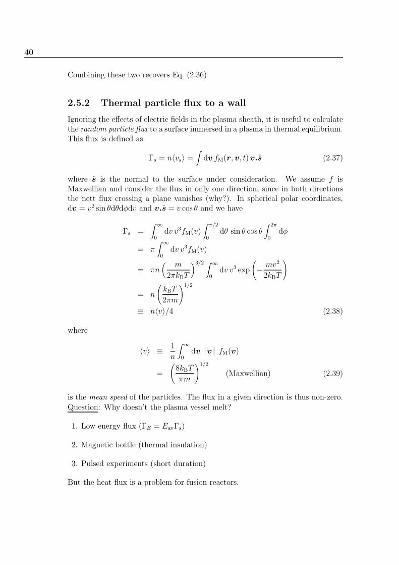
2.5.2 Thermal particle flux to a wall

Ignoring the effects of electric fields in the plasma sheath, it is useful to calculatethe random particle flux to a surface immersed in a plasma in thermal equilibrium.This flux is defined as

Γs = n〈vs〉 =∫

dv fM(r, v, t) v.s (2.37)

where s is the normal to the surface under consideration. We assume f isMaxwellian and consider the flux in only one direction, since in both directionsthe nett flux crossing a plane vanishes (why?). In spherical polar coordinates,dv = v2 sin θdθdφdv and v.s = v cos θ and we have

Γs =∫ ∞

0dv v3fM(v)

∫ π/2

0dθ sin θ cos θ

∫ 2π

0dφ

= π∫ ∞

0dv v3fM(v)

= πn(

m

2πkBT

)3/2 ∫ ∞

0dv v3 exp

(− mv2

2kBT

)

= n

(kBT

2πm

)1/2

≡ n〈v〉/4 (2.38)

where

〈v〉 ≡ 1

n

∫ ∞

0dv |v | fM(v)

=

(8kBT

πm

)1/2

(Maxwellian) (2.39)

is the mean speed of the particles. The flux in a given direction is thus non-zero.

Question: Why doesn’t the plasma vessel melt?

1. Low energy flux (ΓE = EavΓs)

2. Magnetic bottle (thermal insulation)

3. Pulsed experiments (short duration)

But the heat flux is a problem for fusion reactors.

2.5 Maxwell-Boltzmann Distribution 41

2.5.3 Local Maxwellian distribution

We define the local Maxwellian velocity distribution as

fLM(v) = n(

m

2πkBT

)3/2

exp

(− mv2

2kBT

)(2.40)

where now

n ≡ n(r, t)

T ≡ T (r, t)

depend on the spatial coordinates and time. fLM can be shown to satisfy theBoltzmann equation. Though each species in a plasma is characterised by itsown distribution function, the time evolution of these distributions are coupledby collisions between the species and the self-consistent electric field that arisesthrough particle diffusion.

2.5.4 The effect of an electric field

Till now we have implicitly ignored the influence of electric fields upon the dis-tribution function. When more than a single particle species (for example ionsand electrons) are considered, however, such fields can arise spontaneously in theplasma due to differences in the mobility or transport of the two species. Theelectric field in turn affects the spatial distribution of particle velocities throughthe Lorentz force (we here ignore complications due to magnetic fields). Thiseffect is important for the electrons owing to their much greater mobility. Thespatial variation of the electric potential (E = −∇φ) suggests the use of theconcept of a local Maxwellian.

In equilibrium (∂/∂t = 0) and for B = 0, the Boltzmann equation for elec-trons becomes

v.∇rfe − e

mE.∇vfe = 0. (2.41)

It can be verified by substitution that, in thermal equilibrium, the electron dis-tribution function differs from Maxwellian by a factor related to the electricpotential:

fe = fLM exp

(eφ

kBTe

). (2.42)

The exponent is independent of v so that integration over v gives the Boltzmannrelation

ne = ne0 exp

(eφ

kBTe

)(2.43)

42

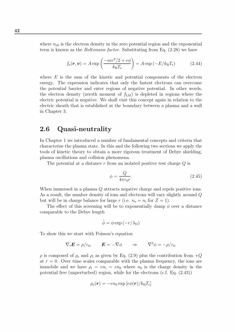
where ne0 is the electron density in the zero potential region and the exponentialterm is known as the Boltzmann factor. Substituting from Eq. (2.28) we have

fe(r, v) = A exp

(−mv2/2 + eφ

kBTe

)= A exp (−E/kBTe) (2.44)

where E is the sum of the kinetic and potential components of the electronenergy. The expression indicates that only the fastest electrons can overcomethe potential barrier and enter regions of negative potential. In other words,the electron density (zeroth moment of fLM) is depleted in regions where theelectric potential is negative. We shall visit this concept again in relation to theelectric sheath that is established at the boundary between a plasma and a wallin Chapter 3.

2.6 Quasi-neutrality

In Chapter 1 we introduced a number of fundamental concepts and criteria thatcharacterise the plasma state. In this and the following two sections we apply thetools of kinetic theory to obtain a more rigorous treatment of Debye shielding,plasma oscillations and collision phenomena.

The potential at a distance r from an isolated positive test charge Q is

φ =Q

4πε0r. (2.45)

When immersed in a plasma Q attracts negative charge and repels positive ions.As a result, the number density of ions and electrons will vary slightly around Qbut will be in charge balance for large r (i.e. ne = ni for Z = 1).

The effect of this screening will be to exponentially damp φ over a distancecomparable to the Debye length

φ = φ exp (−r/λD)

To show this we start with Poisson’s equation

∇.E = ρ/ε0, E = −∇φ ⇒ ∇2φ = −ρ/ε0.

ρ is composed of ρe and ρi as given by Eq. (2.9) plus the contribution from +Qat r = 0. Over time scales comparable with the plasma frequency, the ions areimmobile and we have ρi = eni = en0 where n0 is the charge density in thepotential free (unperturbed) region, while for the electrons (c.f. Eq. (2.43))

ρe(r) = −en0 exp [eφ(r)/kBTe]

2.6 Quasi-neutrality 43

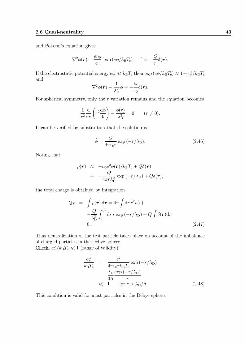
and Poisson’s equation gives

∇2φ(r) − en0

ε0[exp (eφ/kBTe) − 1] = −Q

ε0δ(r).

If the electrostatic potential energy eφ � kBTe then exp (eφ/kBTe) ≈ 1+eφ/kBTe

and

∇2φ(r) − 1

λ2D

φ = −Q

ε0δ(r).

For spherical symmetry, only the r variation remains and the equation becomes

1

r2

d

dr

(r2dφ

dr

)− φ(r)

λ2D

= 0 (r �= 0).

It can be verified by substitution that the solution is

φ =Q

4πε0rexp (−r/λD). (2.46)

Noting that

ρ(r) ≈ −n0e2φ(r)/kBTe + Qδ(r)

= − Q

4πrλ2D

exp (−r/λD) + Qδ(r),

the total charge is obtained by integration

QT =∫

ρ(r) dr = 4π∫

dr r2ρ(r)

= − Q

λ2D

∫ ∞

0dr r exp (−r/λD) + Q

∫δ(r)dr

= 0. (2.47)

Thus neutralization of the test particle takes place on account of the imbalanceof charged particles in the Debye sphere.

Check: eφ/kBTe � 1 (range of validity)

eφ

kBTe

=e2

4πε0rkBTe

exp (−r/λD)

=λD

3Λ

exp (−r/λD)

r� 1 for r > λD/Λ (2.48)

This condition is valid for most particles in the Debye sphere.

44

Figure 2.5: Electrostatic Coulomb potential and Debye potential as a function of

distance from a test charge Q.

2.7 Kinetic Theory of Electron Waves

As another example of the importance of a kinetic theory, we consider the de-scription of electron plasma oscillations (waves) in a warm plasma. When thermaleffects (a distribution of velocities) are included in the treatment of plasma oscil-lations, it is found that the disturbances, which were found to be pure oscillationsin Sec 1.1.2, do indeed propagate and are strongly damped by a linear collisionlessmechanism known as Landau damping after the Soviet physicist who predicted itmathematically in 1946. The analysis presented here closely follows those givenin [3, 4].

To describe these phenomena, we consider a simple one-dimensional system,ignore collisions and assume no magnetic field. Because of their much greaterinertia, we regard the ions as providing a fixed uniform background at frequenciesnear ωpe. The Vlasov equation can be written

∂f

∂t+ v

∂f

∂x+

qE

m

∂f

∂v= 0. (2.49)

In the presence of a wave, we allow the equilibrium distribution function f0 to beperturbed an amount f1 with an associated small electric field E = E1 due to thedisturbance. Substituting f = f0 + f1 into the 1-D Valsov equation, expanding

2.7 Kinetic Theory of Electron Waves 45

and retaining terms up to first order in small quantities gives

∂f1

∂t+ v

∂f1

∂x+

qE

m

∂f0

∂v= 0. (2.50)

We assume a plane harmonic form for the response f1 ∼ exp (ikx − iωt) to theinitial one-dimensional perturbation, recognizing that ω may be complex in orderto allow for wave damping. This allows the substitutions

∂

∂t→ −iω (2.51)

∂

∂x→ ik (2.52)

to obtain

−iωf1 + ikvf1 +qE

m

∂f0

∂v= 0. (2.53)

(We have implicitly integrated f over the velocity variables orthogonal to v, sothat f is one-dimensional.) Solving for the perturbation gives

f1 = −qE

im

∂f0/∂v

kv − ω. (2.54)

By analogy with Eq. (2.7) the perturbed density is given by

n1 = −qE

im

∫ ∞

−∞dv

∂f0/∂v

kv − ω. (2.55)

This in turn gives rise to an electric potential fluctuation φ1 that can be obtainedusing E1 = −∂φ1/∂x and Poisson’s equation ∂E/∂x = qn1/ε0. Substituting inEq. (2.55) gives the dispersion relation (a relation linking the phase velocity ofthe wave to its frequency and wavenumber)

1 = −ω2pe

k2

∫ ∞

−∞dv

∂f0/∂v

(v − ω/k). (2.56)

We have normalized the unperturbed distribution function to the electron numberdensity f0 = f0/n (see Eq. (2.10)) and used Eq. (1.14) for the plasma frequency.Note that the integrand contains a singularity at vph = ω/k and the integralrequires to be evaluated using contour integration in the complex plane. However,the correct result can also be obtained using the less rigorous approach describedbelow.

Fig. 2.6 shows the distribution f0(v) and the integrand. Assuming vph >>vthe, the latter can be conveniently separated into two parts

(i) the central region dominated by ∂f0/∂v

(ii) the region near v = vph dominated by the singularity

46

Figure 2.6: The contributions (i) and (ii) noted in the text [3]

Contribution of the central region

In this region, v � vph, allowing the integrand to be expanded in powers of v/vph

to give for the integral:

− 1

vph

∫ ∞

−∞dv

∂f0/∂v

1 − v/vph

= − 1

vph

∫ ∞

−∞dv

∂f0

∂v

1 +

v

vph

+

(v

vph

)2

+

(v

vph

)3

+ . . .

≈ − 1

v2ph

∫ ∞

−∞dv v

∂f0

∂v− 1

v4ph

∫ ∞

−∞dv v3 ∂f0

∂v(2.57)

where we have truncated the series after the two most significant terms (the termscontaining even powers of v are zero by the antisymmetry of the integrand). Theseintegrals can be evaluated by parts and substituted into Eq. (2.56) to obtain

1 =ω2

pe

ω2

(1 +

3k2

ω2v2

)

where we have made use of the definition of the mean square particle speed andignored the contribution from the singularity. For f0 Maxwellian, we have

1

2mv2 =

1

2kBT

and the above can be solved for ω2 in terms of k2 to obtain (show this)

ω2 ≈ ω2pe +

3kBT

mk2. (2.58)

This is the so-called Bohm-Gross dispersion relation for electron plasma waves(or Langmuir waves). The inclusion of finite electron temperature has contributed

2.7 Kinetic Theory of Electron Waves 47

a propagating component (k-dependent) to the dispersion relation. This resultcan also be obtained using the fluid equations (Chapter ??) which describe theevolution of distribution averaged quantities. Some important non-equilibriumphysical effects (such as Landau damping) are lost in this averaging process. Itis the remaining integral over the singularity that reveals this.

Contribution of the singularity

Within a narrow range of velocity around the singularity, we may regard ∂f0/∂vas constant and remove it from the integral. With u = v − ω/k, the integral canbe written

ω2pe

k2

(∂f0

∂v

)ω/k

∫ ∞

−∞du

u(2.59)

Now ∫ a

−a

du

u= ln a − ln−a = ln a − ln [a exp (iπ + i2πn)]

= ln a − ln a − (iπ + i2πn)

= −iπ (2.60)

where we have taken n = 0. Thus the singularity component becomes

−iπω2

pe

k2

(∂f0

∂v

)ω/k

(2.61)

and the full dispersion relation for electron plasma waves is

1 =ω2

pe

ω2

(1 +

3k2

ω2v2

)− iπ

ω2pe

k2

(∂f0

∂v

)ω/k

(2.62)

Treating the imaginary part (damping term) as small, and neglecting the thermalcorrection, we can use Taylor’s theorem and rearrange to obtain (Prove thisresult)

ω = ωpe

1 + i

π

2

ω2pe

k2

(∂f0

∂v

)ω/k

(2.63)

It is left as an exercise to show that if f0 is a one-dimensional Maxwellian, thedamping is finally given by

Im

(ω

ωpe

)= −0.22

√π(

ωpe

kvth

)2

exp

( −1

2k2λ2D

)(2.64)

where λD is given by Eq. (1.15). Since Im(ω) is negative, the wave is damped, theeffect becoming important for waves of wavelength smaller or comparable withthe Debye length.

48

2.7.1 The physics of Landau damping

We have noted the appearance of a small electric field associated with the elec-tron wave and an accompanying disturbance of the distribution from thermalequilibrium. The Boltzmann relation requires that the density varies with theelectric potential according to Eq. (2.43). This is shown schematically in Fig.2.7 where is plotted the potential energy qφ = −eφ of an electron in an electronplasma wave. Thus, at the wave potential energy peaks, the electron density islower than in the troughs.

Figure 2.7: Diagram showing the electron potential energy −eφ in an electron

plasma wave. Regions labelled A accelerate the electron while in B, the electron

is decelerated [3].

Now consider electrons at the potential energy peak moving with velocityslightly faster than the phase velocity of the wave. These electrons will be accel-erate, sacrificing potential for kinetic energy. Those particles in the trough willbe decelerated. However, there are more particles in the trough than at the peak,so the net effect is deceleration and the electrons give energy to the wave.

This argument can be inverted, however, by considering electrons movingslightly slower than the wave. The net effect is opposite: the wave gives energyto the electrons. There is remaining, however, a fundamental asymmetry in thatthere are more particles moving slower than the wave velocity vph than goingfaster due to the slope of the distribution function. Thus, overall, there is a netloss of energy by the wave which is damped and a corresponding modification ofthe distribution function around v = vph. There is no dissipation inherent in theprocess. However, collisions will cause the perturbed distribution to relax backto Maxwellian in the absence of a source for the wave excitation which couldmaintain the perturbation.

2.8 Collision Processes 49

2.8 Collision Processes

Collisions mediate the transfer of energy and momentum between various speciesin a plasma, and as we shall see later, allow a treatment of highly ionized plasmaas a single conducting fluid with resistivity determined by electron-ion collisions.

Collisions which conserve total kinetic energy are called elastic. Some exam-ples are atom-atom, electron-atom, ion-atom (charge exchange) etc. In inelas-tic collisions, there is some exchange between potential and kinetic energies ofthe system. Examples are electron-impact ionization/excitation, collisions withsurfaces etc. In this section, we consider both types of collision process, withparticular emphasis on Coulomb collisions between charged particles, this beingthe dominant process in a plasma.

A simple expression for the collision term on the right of Eq. (2.5) is the Krookcollision term (

∂f

∂t

)coll

= −(

f − fM

τ

)(2.65)

where fM is the Maxwellian towards which the system is tending and τ is themean (constant) collision time. The model integrates to give

f(t) = fM + (f(0) − fM) exp (−t/τ). (2.66)

The model is not very good if the masses of the species are very different.

2.8.1 Fokker-Planck equation

2.8.2 Mean free path and cross-section

To properly treat the physics of collisions we need to introduce the concept ofmean free path - a measure of the likelihood of a collision event. Imagine electronsimpinging on a box of neutral gas of cross-sectional area A (see Fig 2.8).

If there are nn atoms m−3 in volume element Adx the total area of atoms inthe volume (viewed along the x-axis) is nnAdxσ where σ is the cross-section andnnAdxσ � A so that there is no “shadowing”. The fraction of particles makinga collision is thus nnAdxσ/A - the fraction of the cross-section blocked by atoms.If Γ is the incident particle flux, the emerging flux is Γ′ = Γ(1 − nnσdx) and thechange of Γ with distance is described by

dΓ

dx= −nnσΓ. (2.67)

The solution is

Γ = Γ0 exp (−x/λmfp)

λmfp =1

nnσ(2.68)

50

dx

Area A n atoms/cm3

x

Incoming particle

Figure 2.8: Particles moving from the left and impinging on a gas undergo colli-

sions.

where λmfp is the mean free path for collisions characterised by the cross-sectionσ. The physics of the interaction is carried by σ, the rest is geometry.

The mean free time between collisions, or collision time for particles of ve-locity v is τ = λmfp/v and the collision frequency is ν = τ−1 = v/λmfp = nnσv.Averaging over all of the velocities in the distribution gives the average collisionfrequency

ν = nnσv (2.69)

where we have allowed for the fact that σ can be energy dependent as we shallsee below.

2.8.3 Coulomb collisions

Coulomb collisions between free particles in a plasma is an elastic process. Letus consider the Coulomb force between two test charges q and Q

F =qQ

4πε0r2≡ C

r2(2.70)

This is a long range force and the cross-section for inetraction of isolated chargesis infinity! It is quite different from elastic “hard-sphere” encounters such asthat which can occur between electrons and neutrals for example. In a plasma,however, the Debye shielding limits the range of the force so that an effectivecross-section can be found. Nevertheless, because of the nature of the force, themost frequent Coulomb deflections result in only a small deviation of the particlepath before it encounters another free charge. To produce an effective 90◦ scat-tering of the particle (and hence momentum transfer) requires an accumulationof many such glancing collisions. The collision cross-section is then calculated bythe statistical analysis of many such small-angle encounters.

2.8 Collision Processes 51

Consider the force Eq. (2.70) on an electron as it follows the unperturbed pathshown in Fig. 2.9 In this picture, only the perpendicular component mattersbecause the parallel compoent of the force reverses direction after q passes Q.Thus F⊥/F = b/r or

F⊥ = Cb/r3 =cb

(x2 + b2)3/2

where b is the impact parameter for the interaction. Since x (the parallel coordi-nate) changes with time, we integrate along the path to obtain the net perpen-dicular impulse delivered to q

δ(mv⊥) =∫ ∞

−∞F⊥dt = cb

∫ ∞

−∞dx

(x2 + b2)3/2

dt

dx

F

xq

Q

bImpactparameter

Unperturbed path

Figure 2.9: The trajectory taken by an electron as it makes a glancing impact

with a massive test charge Q

Now ∫dx

(x2 + b2)3/2=

x

b2(x2 + b2)1/2

→ −1/b2 x → −∞→ 1/b2 x → ∞

so that

δv⊥ =2c

mvb. (2.71)

We consider a statistical average over a random distribution of such smallangle collisions. For a random walk with step length δs, the total displacementafter N steps is ∆s =

√Nδs (i.e. (∆s)2 =

∑(δs)2) where N is the number of

steps. The total change in velocity is thus

(∆v⊥)2 = N(δv⊥)2. (2.72)

52

Now integrate over the range of impact parameters b to estimate the number ofglancing collisions in time t. Small angle colisions are much less likely because ofthe geometrical effect

N(b) = n(2πbdb)vt. (2.73)

We combine equations (2.71), (2.72) and (2.73) and integrate over impact param-eter:

(∆v⊥)2 =8πnC2t

m2v

∫ bmax

bmin

db

b. (2.74)

bmin is the closest approach that satisfies the small deflection hypothesis. Weobtain this be setting δv⊥ = v

bmin =2c

mv2=

2qQ

4πε0mv2. (2.75)

Outside λD the charge Q is not felt. We thus take bmax = λD and

∫ bmax

bmin

db

b= ln

(λD

bmin

)= ln Λ.

ln Λ is called the Coulomb logarithm and is a slowly varying function of electrondensity and temperature. For fusion plasma ln Λ ∼ 6 − 16. One usually setsln Λ = 10 in quantitative estimations.

We are finally in a position to find the elapsed time necessary for a net 90◦

deflection i.e. (∆v⊥)2 = v2. Using Eq. (2.74)

(∆v⊥)2 = v2 =8πnc2t

m2vln Λ

and

ν90 = 1/t =8πnq2Q2 ln Λ

16π2ε20m

2v3.

For electron-ion encounters, q = −e and Q = Ze so

ν90ei ≡ νei =niZ

2e4 ln Λ

2πε20m

2v3(2.76)

and νei = niσeiv implies that

σei =Z2e4 ln Λ

2πε20m

2v4(2.77)

Let’s review this derivation

• Perpendicular impulse ∼ 1/vb

• Angular deflection ∆θ ∼ δv⊥/v ∼ 1/v2

2.8 Collision Processes 53

• Random walk to scatter one radian (∆v/v = 1) ∼ 1/(∆θ)2 → σ ∼ 1/v4

• Integrate over b → ln Λ.

The dependence σ ∼ 1/v4 has very important ramifications. A high temperatureplasma is essentially collisionless. This means that plasma resistance decreasesas temperature increases. In some circumstances populations of particles canbe continually accelerated, losing energy only through synchrotron radiation (forexample runaway electrons in a tokamak).

Energy transfer in electron-ion collisions

A pervading theme in plasma physics is me � mi. This has consequences forcollisions between the species in that we expect very little energy transfer betweenthe species. To illustrate this, consider such a collision in the centre-of-mass frame(a direct hit).

m M

After

Before

Vv

v0V0

Figure 2.10: Collison between ion and electron in centre of mass frame.

mv0 + MV0 = 0 = mv + MV momentum

mv20 + MV 2

0 = mv2 + MV 2 energy

mv20

(1 +

m

M

)= mv2

(1 +

m

M

)eliminate V

⇒ v = ±v0 and V = ±V0. (2.78)

Now translate to frame in which ion M is at rest (initially). In this frame theinitial electron energy is

Ee0 =1

2m(v0 − V0)

2 =1

2mv2

0

(1 +

m

M

)2

and the final ion energy is

Ei =1

2M(2V0)

2 = 2M

(m2v2

0

M2

).

54

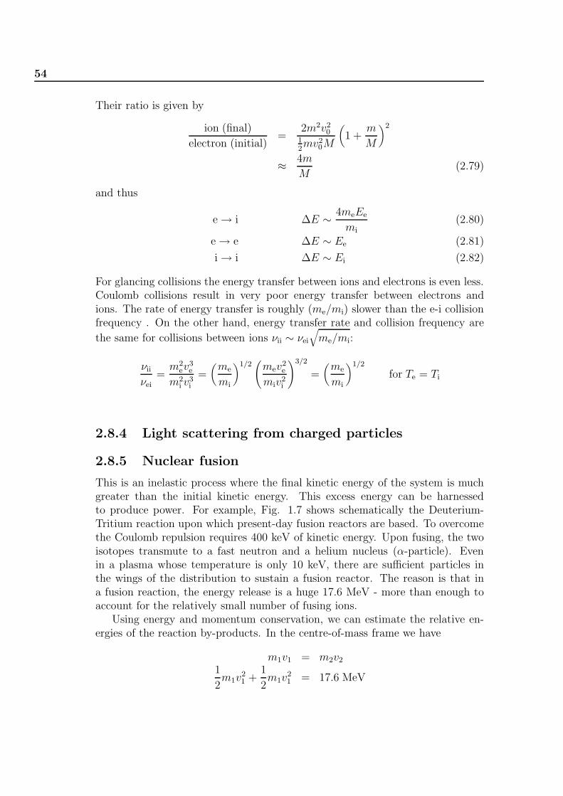
Their ratio is given by

ion (final)

electron (initial)=

2m2v20

12mv2

0M

(1 +

m

M

)2

≈ 4m

M(2.79)

and thus

e → i ∆E ∼ 4meEe

mi

(2.80)

e → e ∆E ∼ Ee (2.81)

i → i ∆E ∼ Ei (2.82)

For glancing collisions the energy transfer between ions and electrons is even less.Coulomb collisions result in very poor energy transfer between electrons andions. The rate of energy transfer is roughly (me/mi) slower than the e-i collisionfrequency . On the other hand, energy transfer rate and collision frequency are

the same for collisions between ions νii ∼ νei

√me/mi:

νii

νei=

m2ev

3e

m2i v

3i

=(

me

mi

)1/2(

mev2e

miv2i

)3/2

=(

me

mi

)1/2

for Te = Ti

2.8.4 Light scattering from charged particles

2.8.5 Nuclear fusion

This is an inelastic process where the final kinetic energy of the system is muchgreater than the initial kinetic energy. This excess energy can be harnessedto produce power. For example, Fig. 1.7 shows schematically the Deuterium-Tritium reaction upon which present-day fusion reactors are based. To overcomethe Coulomb repulsion requires 400 keV of kinetic energy. Upon fusing, the twoisotopes transmute to a fast neutron and a helium nucleus (α-particle). Evenin a plasma whose temperature is only 10 keV, there are sufficient particles inthe wings of the distribution to sustain a fusion reactor. The reason is that ina fusion reaction, the energy release is a huge 17.6 MeV - more than enough toaccount for the relatively small number of fusing ions.

Using energy and momentum conservation, we can estimate the relative en-ergies of the reaction by-products. In the centre-of-mass frame we have

m1v1 = m2v2

1

2m1v

21 +

1

2m1v

21 = 17.6 MeV

2.8 Collision Processes 55

where subscripts 1 and 2 refer respectively to the α-particle and the neutron.Eliminating v1 gives

1

2m2v

22

(1 +

m2

m1

)= 17.6 MeV.

Substituting m2/m1 = 1/4 shows that 14.1 MeV is carried by the neutron whichescapes the confining magnetic field to deliver useful energy elsewhere. The fastα (3.5 MeV) is confined by the magnetic field where it delivers its energy to thedeuterium and tritium ions.

For the D-T reaction in a high temperature plasma with n ∼ 1 × 1020 m−3

and σ ∼ 10−29 m−2 at 100 keV where v ∼ 5 × 106 m/s, the mean free path for afusion collision is

λmfp =1

nσ= 109 m

and τ = λmfp/v ≈ 200 s. In other words, D and T have to be confined for 200s and travel a million km without hitting the container walls! The situation ismitigated by the fact that 17.6 MeV 10 keV so that not all particles need tofuse in order to achieve a net energy gain.

2.8.6 Photoionization and excitation

To understand these processes, we must first look at the atomic physics of the H-atom. This is governed by the Coulomb force. Taking a semi-classical approach,we may equate the centripetal force with the Coulomb attraction

F =mv2

r=

e2

4πε0r2.

The kinetic energy of the electron is 12mv2 = e2/(8πε0r) and the potential en-

ergy is −e2/(4πε0r) so that the total energy of the atomic system is KE+PE =−e2/(8πε0r) (it is a bound system).

Given that electrons are bound in states having de Broglie wavelength satis-fying nλ = 2πr, we may obtain for the energies of the bound states

En = −13.6 eV/n2 n = 1, 2, 3, . . .

(To see this, we write nh = hkr = mvr, or r = nh/mv and substitute into theexpression for the kinetic energy to obtain r = (n2/Z)a0 where a0 is the Bohrradius. This is finally subsituted into the expression for the total energy of theatom.) It is clear that the energy required to ionize the H atom is 13.6 eV andto excite from the ground state is E2 − E1 = 10.2 eV. Photons of these energiesreside in the deep ultarviolet of the spectrum. Since the photon energy is usedto disrupt a bound system, this is an inelastic process.

56

2.8.7 Electron impact ionization

The area of the hydrogen atom is πa20 = 0.88 × 10−20m−2. If an electron comes

within a radius a0 of the atom and has energy in excess of 13.6 eV, ionizationwill probably result. The behaviour of the electron impact ioization cross-sectionas a function of electron energy is shown in Fig. 2.11.

Figure 2.11: The electron impact ionization cross-section for hydrogen as a func-

tion of electron energy. Note the turn-on at 13.6 eV. [2]

The cross-section falls for energies greater than 100 eV since the electron doesnot spend much time in the vicinity of the atom. The cross section, averagedover the distribution of electron velocities, can be used to estimate the electronmean free path for a given neutral density. Again this is an inelastic process.

2.8.8 Collisions with surfaces

Reactions with surfaces are complex. Gases are readily adsorbed on a cleansurface, sticking with probability 0.3 to 0.5 to form a “monolayer” surface. Thebinding energy is a strong function of the type of gas however, being smallestfor the noble gases. Heating at temperatures >∼ 2000◦ will usually produce anatomically clean surface in <∼ 1 sec.

Secondary emission by electrons

Electrons striking a surface can, if their energy exceeds that of the surface workfunction, eject other electrons. The emission coefficient falls at high energies be-cause the incident electron penetrates too deeply and secondaries cannot escape.

2.9 Fluid Equations 57

At low energies, the released electron energy is less than the work function and itcannot escape. At intermediate energies we can have δ > 1 (gain). The shape ofthe plot of secondary emission coefficient δ (number of electrons emitted for eachincident electron) versus incident energy is similar for all materials. Because ofthe mass difference, electrons have low probability of ejecting atoms.

Figure 2.12: Electron secondary emission for normal incidence on a typical metal

surface [2]

Secondary electron emission by ions

The number of secondary electrons emitted per positive ion is denoted γi. Typi-cally γi < 0.3 and is roughly independent of the ion speed.

2.9 Fluid Equations

Just as the velocity moments of the distribution function give important macro-scopic variables, so the velocity moments of the plasma kinetic equation (Boltz-mann equation Eq. (2.5)) give the equations that describe the time evolution ofthese macroscopic parameters. Because these equations (apart from the Lorentzforce) are identical with the continuum hydrodynamic equations, the theoriesusing the low-order moments are called fluid theories. Remember that the fluidequations can be applied separately to each of the species that constitute theplasma.

58

2.9.1 Continuity—particle conservation

The equation of continuity is derived from the zeroth velocity moment of theBoltzmann equation. Its analogue for the particle distribution function is justthe number density. It is not surprising that continuity describes conservation ofparticle number. We shall derive the moment equations only for the zeroth mo-ment and simply state the result for the higher order moments of the Boltzmannequation.

Since v0 = 1, the zeroth order moment implies a simple integration overvelocity space to obtain

∫∂f

∂tdv +

∫v.∇rfdv +

q

m

∫(E + v×B).∇vfdv =

∫ (∂f

∂t

)coll

dv (2.83)

The first term gives ∫∂f

∂tdv =

∂

∂t

∫fdv =

∂n

∂t. (2.84)

Since v is independent of r (independent variables) the second term gives∫v.∇rfdv = ∇r.

∫vfdv = ∇.(nv) ≡ ∇.(nu) (2.85)

where we have used Eq. (2.14) and defined u as the “fluid” velocity. The terminvolving E in the third integral vanishes:

∫E.

∂f

∂vdv =

∫∂

∂v.(fE)dv =

∫S∞

fE.dS = 0 (2.86)

where the surface S∞ is the v-space surface at v → ∞. The first step is validbecause E is independent of v while the second is an application of Gauss’ vectorintegral theorem. This last integral vanishes because f vanishes faster than v−2

(area varies as 4πv2) as v → ∞ (i.e. finite energy system). The v×B componentcan be written∫

(v×B).∂f

∂vdv =

∫ ∂

∂v.(fv×B)dv −

∫f

∂

∂v×(v×B)dv = 0 (2.87)

The second term can be transformed to a surface integral which again vaishes atinfinity. Because ∂/∂v and v×B are mutually perpendicular, the second righthand term also vanishes. Finally, the 4th term of Eq. (2.83) vanishes becausecollisions cannot change the number of particles (at least for warm plasmas,where recombination can be ignored). The final result is

∂n

∂t+ ∇.(nu) = 0 (2.88)

which expresses conservation of particles . Multiplying by m or q yields conser-vation of mass or charge.

2.9 Fluid Equations 59

Note that taking the zeroth moment of the Boltzmann equation has intro-duced a higher order moment u — the first velocity moment of f . Its descriptionwill require taking the first order moment of the Boltzmann equation. As we shallsee, this will in turn generate second order moments and so on. This is knownas the closure problem. At some stage, the sequence must be terminated bysome reasonable procedure. Usually this is effected by setting the third velocitymoment of f (describing the thermal conductivity) to zero.

2.9.2 Fluid equation of motion

The first moment equation (multiply by mv the particle momentum and inte-grate) expresses conservation of momentum. The resulting equation of motion isgiven by

mn

[∂u

∂t+ (u.∇)u

]= qn(E + u×B) −∇.

↔P +Pcoll (2.89)

where the left hand side will be recognized as proportional to the convectivederivative of the average velocity u. The right side includes the Lorentz force,the divergence of the pressure tensor (a second order quantity) and the exchangeof momentum due to collisions with other species in the plasma:

Pcoll =∫

mv

(∂f

∂t

)coll

dv =

[∂

∂t

∫mvfdv

]coll

(2.90)

Collisions between like particles cannot produce a net change of momentum ofthat species.

Pressure tensor

The elements of the pressure tensor are defined by Eq. (2.16) such that Pij =mnvivj . For an isotropic Maxwellian distribution,

↔P=

p 0 00 p 00 0 p

(2.91)

and ∇.↔P= ∇P where P = mnv2

r/3 = nkT is the scalar pressure. In thepresence of a magnetic field, isotropy can be lost and the species may assumedistict temperatures along and across the magnetic field so that p‖ = nkT‖ andp⊥ = nkT⊥ with

↔P=

p⊥ 0 0

0 p⊥ 00 0 p‖

where it is customary to take the z direction to conincide with the direction ofB. Note that the pressure is still isotropic in the plane normal to B.

60

The collision term

If a species α (for example electrons) is interacting with another via collisions,the momentum lost per collision will be proportional to the relative fluid velocityuα−uβ where β denotes the “background” fluid (for example ions or neutrals). Ifthe mean free time between collisions τ is approximately constant, the resultingfrictional drag term can be written as

Pei = −mene(ue − ui)

τei(2.92)

where Pei is the force felt by the electron fluid flowing with velocity ue−ui relativeto the background (in this case ion) fluid. By conservation of momentum, themomentum lost (gained) through collisions by the electrons on ions must equalthe momentum gained (lost) by the ions. Thus

Pei = −Pie. (2.93)

What does this say about νie compared with νei?

2.9.3 Equation of state

The second moment equation describes conservation of energy. It is derived bymultiplying the Boltzmann equation by mv2/2 and integrating over velocity. Theresult is

∂

∂t

(nm

2v2)

+ ∇r.(

nm

2vv2

)= j.E +

∫dv

nm

v2

(∂f

∂t

)coll

. (2.94)

The left hand side terms represent the change of energy density with time and theenergy flow across the surface bounding the volume element of interest. The sumof these two terms equals the electric power dissipated in the plasma plus anyenergy that might be generated per unit time through collisions. The magneticfield does no work because it always acts in a direction perpendicular to theparticle velocity.

The equation can be dramatically simplified under the assumption that thedistribution function is a drifting Maxwellian (v = u+vr where vr is the randomor thermal velocity component) and provided collisions do not create new par-ticles (ionization) or change the temperature (thermal conductivity = 0). Thiscorresponds to a system undergoing adiabatic changes (no heat flow). The secondmoment equation then becomes the equation of state:

dp

dn=

5p

3n(2.95)

On integration this givesp = p0n

5/3. (2.96)

2.9 Fluid Equations 61

More generally, we can writep = Cργ (2.97)

where C is a constant,γ = (2 + N)/N (2.98)

is the ratio of specific heats (Cp/CV ) and N is the number of degrees of freedom.In 3-D, N = 3, γ = 5/3 and we recover Eq. (2.96). Equation (2.97) can also bewritten as

∇p

p= γ

∇n

n(2.99)

or ∇p = γkBT ∇n (2.100)

For the isothermal case (T=constant, thermal conductivity infinite) we have

∇p = ∇(nkBT ) = kBT∇n (2.101)

and γ = 1

2.9.4 The complete set of fluid equations

Let us define

σ = niqi + neqe (2.102)

j = niqiui + neqeue (2.103)

as net charge and current densities respecticely. Ignoring collisions and viscosity(i.e. the pressure tensor → scalar pressure p) we have fluid equations for speciesj = i, e

∂nj

∂t+ ∇.(njuj) = 0 (2.104)

mjnj

[∂uj

∂t+ (uj.∇)uj

]= qjnj(E + uj×B) −∇pj (2.105)

pj = Cjnγj

j (2.106)

supplemented by Maxwell’s equations for the field

∇.E =σ

ε0(2.107)

∇×E = −∂B

∂t(2.108)

∇.B = 0 (2.109)

∇×B = µ0j + µ0ε0∂E

∂t. (2.110)

These two sets of equations provide 16 independent equations for the 16 unknownsni, ne, pi, pe, ui, ue, E and B. Two of Maxwell’s equations are redundant. In thiscourse we shall examine and employ these equations to solve a range of simpleplasma physics problems.

62

2.9.5 The plasma approximation

In many plasma applications it is usually possible to assume ni = ne and ∇.E �= 0at the same time. On time scales slow enough for the ions and electrons to move,Poisson’s equation can be replaced by ni = ne (i.e. quasi-neutrality). Poisson’sequation holds for electrostatic applications:

∂B

∂t= 0 ⇒ ∇×E = 0 ⇒ E = −∇φ ⇒ ∇2φ = −σ/ε0.

The electric field can be found from the equations of motion. If necessary, thecharge density can then be found from Poisson’s equation. but it is usually verysmall. This, so-called “plasma approximation” is only valid for low frequencyapplications. For high frequency electron waves, for example, where charges canseparate, it is not a valid approximation.

Problems

Problem 2.1 A chamber of volume 0.5 m3 is filled with hydrogen at a pressure of

10 Pa at room temperature (20◦. Calculate

(a) The number of H2 molecules in the chamber

(b) the mass of the gas in the chamber (proton mass = 1.67 × 1027 kg)

(c) the average kinetic energy of the molecules

(d) the RMS speed of the molecules

(e) the energy in Joules required to heat the gas to 100,000 K, given that it takes 2

eV to dissociate a H2 molecule into H atoms and 13.6 eV to ionize each atom.

Assume that Te = Ti and that the plasma is fully ionized.

(f) the total plasma pressure when Te = Ti = 105K

(g) the RMS speeds of the ions and electrons when Te = Ti = 105K

(h) The electron plasma frequency ωpe, Debye length λD, number of particles in the

Debye sphere ND and the ion-electron collision frequency νei.

Problem 2.2 In the two dimensional phase space (x, v), show the trajectory of

a particle at rest, moving with constant velocity, accelerating at a constant rate,

executing simple harmonic motion and damped simple harmonic motion.

2.9 Fluid Equations 63

Problem 2.3 For any distribution f which is isotropic about its drift velocity v,

prove that

vrαvrβ = v2rδαβ/3

where δαβ is the Kronecker delta

Problem 2.4 If a particle of mass m, velocity v, charge q approaches a massive

particle (M → ∞) of like charge q0, show by energy considerations that the distance

of closest approach is 2qq0/(4πε0mv2).

Problem 2.5 Calculate the cross-section σ90 for an electron Coulomb collsion with

an ion which results in at least a 90◦ deflection of the electron from its initial trajectory.

(HINT: This cross-section is πb2 where b is the maximum impact parameter for such

a collision). Show that the ratio σei/σ90 = 2logeΛ where σei is the collsion cross

section calculated in the notes for multiple small angle Coulomb collisions. Comment

on the significance of this result.

Problem 2.6 Consider the motion of charged particles, in one dimension only, in

an electric potential φ(x). Show, by direct substitution, that a function of the form

f = f(mv2/2 + qφ) is a solution of the Boltzmann equation under steady state

conditions.

Problem 2.7 Since the Maxwellian velocity distribution is isotropic (independent

of velocity direction) it is of interest to define a distribution of speeds v =| v |. That

is, we want a new function g(v) which describes the numer of particles with speeds

between v and v + dv. Show that the desired distribution of speeds (in 3-d) is

g(v) = 4πv2n(m

2πkT)3/2 exp (−mv2/2kT )

Plot this distribution and calculate the most probable particle speed, or in other words,

the speed for which g(v) is a maximum.

Problem 2.8 Consider the following two-dimensional Maxwellian distribution func-

tion:

f(vx, vy) = n0(m

2πkT) exp [−m(v2

x + v2y)/2kT ]

(a) Verify that n0 represents correctly the particle number density, that is, the number

of particles per unit area. (b) Draw, in 3-d, the surface for this distribution function,

plotting f in terms of vx and vy. Sketch on this surface curves of constant vx,

constant vy and constant f .

64

Problem 2.9 The entropy of a system can be expressed in terms of the distribution

function as

S = −k∫ ∞

−∞

∫ ∞

−∞dr dv f f

Show that the total time derivative of the entropy for a system which obeys the

collisionless Boltzmann equtaion is zero.