Embed Size (px)
Citation preview
Chapter 2
POLYHEDRAL COMBINATORICS
Robert D. CarrDiscrete Mathematics and Algorithms Department, Sandia National [email protected]
Goran KonjevodComputer Science and Engineering Department, Arizona State [email protected]
Abstract Polyhedral combinatorics is a rich mathematical subject motivated byinteger and linear programming. While not exhaustive, this survey cov-ers a variety of interesting topics, so let’s get right to it!
Keywords: combinatorial optimization, integer programming, linear programming,polyhedron, relaxation, separation, duality, compact optimization, pro-jection, lifting, dynamic programming, total dual integrality, integralitygap, approximation algorithms
IntroductionThere exist several excellent books [15, 24, 29, 35, 37] and survey
articles [14, 33, 36] on combinatorial optimization and polyhedral com-binatorics. We do not see our article as a competitor to these fine works.Instead, in the first half of our Chapter, we focus on the very founda-tions of polyhedral theory, attempting to present important conceptsand problems as early as possible. This material is for the most partclassical and we do not trace the original sources. In the second half(Sections 5–7), we present more advanced material in the hope of draw-ing attention to what we believe are some valuable and useful, but lesswell explored, directions in the theory and applications of polyhedralcombinatorics. We also point out a few open questions that we feel havenot been given the consideration they deserve.
2-2 Polyhedral Combinatorics
2.1 Combinatorial Optimization and PolyhedralCombinatorics
Consider an undirected graph G = (V,E) (i.e. where each edge isa set of 2 vertices (endpoints) in no specified order). A cycle C =(V (C), E(C)) in G is a subgraph of G (i.e. a graph with V (C) ⊆ V andE(C) ⊆ E) that is connected, and in which every vertex has degree 2.If V (C) = V , then C is said to be a Hamilton cycle in G. We define thetraveling salesman problem (TSP) as follows. Given an undirected graphG = (V,E) and a cost function c : E → R, find a minimum cost Hamil-ton cycle in G. The TSP is an example of a combinatorial optimizationproblem. In fact, it is an NP-hard optimization problem [31], althoughsome success has been achieved both in approximating the TSP and insolving it exactly [19].
More generally, a combinatorial optimization problem is by definitiona set, and we refer to its elements as instances. Each instance furtherspecifies a finite set of objects called feasible solutions, and with eachsolution there is an associated cost (usually an integer or rational num-ber). Solving an instance of a combinatorial optimization problem meansfinding a feasible solution of minimum (in the case of a minimizationproblem)—or maximum (in the case of a maximization problem)—cost.The solution to a combinatorial optimization problem is an algorithmthat solves each instance.
A first step in solving a combinatorial optimization problem instanceis the choice of representation for the set of feasible solutions. Practi-tioners have settled on representing this set as a set of vectors in a finite-dimensional space over R. The dimension depends on the instance, andthe set of component indices typically has a combinatorial meaning spe-cial to the problem, for example, the edge-set E of a graph G = (V,E)that gives rise to the instance (Section 2.2). However, we sometimes justuse the index set [n] = {1, 2, . . . , n}.
There often are numerous ways to represent feasible solutions as vec-tors in the spirit of the previous paragraph. Which is the best one? It isoften most desirable to choose a vector representation so that the costfunction on the (finite) set of feasible solutions can be extended to alinear function on RI (where I is an index set) that agrees with the costof each feasible solution when evaluated at the vector representing thesolution.
In Theorems 2.1 and 2.2, we give just one concrete reason to strivefor such a linear cost function. But first, some definitions (for thosemissing from this paragraph, see Section 2.2.2). Let S ⊂ RI be a setof vectors (such as the set of all vectors that represent the (finitely
Combinatorial Optimization and Polyhedral Combinatorics 2-3
many) feasible solutions to an instance of a combinatorial optimizationproblem, in some vector representation of the problem instance). Aconvex combination of a finite subset {vi | i ∈ I} of vectors in S is a linearcombination
∑i∈I λiv
i of these vectors such that the scalar multiplier λiis nonnegative for each i (λi ≥ 0) and∑
i∈Iλi = 1.
Geometrically, the set of all convex combinations of two vectors formsthe line segment having these two vectors as endpoints. A convex setof vectors is a set (infinite unless trivial) of vectors that is closed withrespect to taking convex combinations. The convex hull of S (conv(S))is the smallest (with respect to inclusion) convex set that contains S.For a finite S, it can be shown that conv(S) is a bounded set that can beobtained by intersecting a finite number of closed halfspaces. The lattercondition defines the notion of a polyhedron. The first condition (thatthe polyhedron is also bounded) makes it a polytope (see Theorem 2.31).Polyhedra can be specified algebraically, by listing their defining half-spaces using inequalities as in (2.1).
Now, the theorems that justify our mathematical structures.
Theorem 2.1 If the cost function is linear, each minimizer over S isalso a minimizer over conv(S).
Theorem 2.2 (Khachiyan, see the reference [15].) If the cost functionis linear, finding a minimizer over a polyhedron is a polynomially solvableproblem as a function of the size of the input, namely the number of bitsin the algebraic description of the polyhedron (in particular, this will alsodepend on the number of closed halfspaces defining the polyhedron andthe dimension of the space the polyhedron lies in).
Proof: Follows from an analysis of the ellipsoid method or an interiorpoint method.
We refer to any problem of minimizing (maximizing) a linear functionover a polyhedron as a linear programming problem, or just a linearprogram. Often we just use the abbreviation LP.
Consider a combinatorial optimization problem defined by a graphG = (V,E) and a cost function on E. We define the size of this inputto be |V | + |E| and denote it by |G|. Denote the set of feasible solu-tions for an instance where the input graph is G by SG. The followingpossibility, of much interest to polyhedral combinatorics, can occur. Itis usually the case that |SG| grows as an exponential function of |G|. Inthis case, it may be hard to tell whether this combinatorial optimization

2-4 Polyhedral Combinatorics
problem is polynomially solvable. However, it is possible here that boththe number of closed halfspaces defining conv(SG) and the dimension ofthe space that the convex hull conv(SG) lies in grow only as polynomialfunctions of |G|. Hence, if we can find this set of closed halfspaces inpolynomial time, the above theorems allow us to immediately concludethat our optimization problem is polynomially solvable! This polyhedralapproach may not be the most efficient way of solving our problem (andadmittedly, there are annoying technical difficulties to overcome whenthe minimizer found for conv(SG) is not in SG), but it is a sure-firebackup if more combinatorial approaches are not successful. We willfind out later that polynomial solvability is also guaranteed if there ex-ist polynomially many (as a function of |G|) sufficiently well-behavedfamilies of halfspaces defining conv(SG). This involves the concept ofseparation, which we discuss in Section 2.3.2.
2.2 Polytopes in Combinatorial OptimizationLet us recall the traveling salesman problem of the previous section.
When the input graph is undirected, we will refer to the symmetric trav-eling salesman problem (STSP), in contrast to the asymmetric travelingsalesman problem (ATSP) that results when the input graph is directed.(For more on polytopes and polyhedra related to STSP and ATSP seethe surveys by Naddef [28] and Balas and Fischetti [1].) It is conve-nient to assume that the input graph for the STSP is a complete graphKn = (Vn, En) on n vertices for some n ≥ 3. Along with the completegraph assumption, we usually assume that the cost function satisfies thetriangle inequality (i.e. defines a metric on Vn).
Recall that we wish to have a vector representation of Hamilton cyclesso that our cost function is linear. If H is a Hamilton cycle, then thecost c(H) :=
∑e∈E(H) ce. So, we cleverly represent each Hamilton cycle
H in Kn by its edge incidence vector χE(H) defined by
χE(H)e :=
{1 e ∈ E(H),0 e ∈ En \ E(H).
Note that now c(H) = c ·χE(H). Hence, we can extend our cost functionfrom edge incidence vectors of Hamilton cycles to a linear function onthe entire space REn by simply defining c(x) := c · x for each x ∈ REn .
The convex hull of all edge incidence vectors of Hamilton cycles in Kn
is a polytope called STSP (n). We noted earlier that optimizing a lin-ear cost function over STSP (n) can be done in polynomial time in thenumber of closed halfspaces defining the polytope, the dimension of thespace and the maximum number of bits needed to represent any coeffi-
Polytopes in Combinatorial Optimization 2-5
cient in the algebraic description of the halfspaces (the size of the explicitdescription), using linear programming. Unfortunately, every known ex-plicit description of STSP (n) is exponential in size with respect to n.Note that in our representation the vector representing any Hamiltoncycle has only integer values, in fact only values in {0, 1}. This suggeststhe new problems of integer programming (IP) and 0-1 programming.For each of these problems, analyzing the geometry of polytopes is ofvalue. We introduce some geometric concepts related to polyhedra andpolytopes, starting with the notion of a polyhedron’s dimension.
2.2.1 Affine Spaces and DimensionLet S = {vi | i ∈ I} be a set of points in RI , where I is a finite index
set. An affine combination on S is a linear combination∑
i∈I λivi, where
the scalar multipliers λi satisfy∑i∈I
λi = 1.
An affine set (space) is a set which is closed with respect to taking affinecombinations. The affine hull aff(S) of a set S is the smallest (withrespect to inclusion) affine set containing S.
We now give two definitions of affine independence.
Definition 2.3 A finite set S is affinely independent iff for any pointwhich can be expressed as an affine combination of points in S, thisexpression is unique.
For the second definition, we introduce the notion of an affine0 combi-nation on S, which is a linear combination
∑i∈I λiv
i where the scalarmultipliers λi satisfy ∑
i∈Iλi = 0.
Definition 2.4 A finite set S is affinely independent iff the only affine0
combination of points in S that gives the 0 (the origin) is that where thescalar multipliers satisfy λi = 0 for all i ∈ I.
Definition 2.5 A set B is an affine basis of an affine space U if it isaffinely independent and aff(B) = U .
Theorem 2.6 The affine hull aff(S) of a set S of points in a finite-dimensional space RI has an affine basis of cardinality at most |I|+ 1.Furthermore, every affine basis of aff(S) has the same cardinality.
Finally, we can define the dimension of a polyhedron P .
2-6 Polyhedral Combinatorics
Definition 2.7 The dimension dim(P ) of a polyhedron P (or any con-vex set) is defined to be |B| − 1, where B is any affine basis of aff(P ).
For example, consider the one-dimensional case. Any two distinct pointsv1, v2 ∈ RI define a one-dimensional affine space aff{v1, v2} called theline containing v1, v2.
If we replace “affine” in Definition 2.4 by “linear,” and “points” by“vectors,” we get the definition of linear independence:
Definition 2.8 A set of vectors V = {v1, . . . , vk} is linearly indepen-dent, if the only linear combination of vectors in V that gives the 0 vectoris that where the scalar multipliers satisfy λi = 0 for all i ∈ I.
Note that linear independence could also be defined using a propertyanalogous to that of Definition 2.3. Either affine or linear independencecan be used for a development of the notion of dimension:
Theorem 2.9 A set {x1, . . . , xk, xk+1} is affinely independent iff the set{x1 − xk+1, . . . , xk − xk+1} is linearly independent.
As in the definition of an affine space, a linear (vector) space is closedwith respect to linear combinations. Let span(B) denote the smallestset containing all linear combinations of elements of B. There is also anotion of basis for linear spaces:
Definition 2.10 A set B is a linear basis of a linear space U if it islinearly independent and span(B) = U .
Theorem 2.11 The linear space span(S), for a set S of vectors in afinite-dimensional space RI has a linear basis of cardinality at most |I|.Furthermore, every linear basis of span(S) has the same cardinality.
Affine independence turns out to be more useful in polyhedral combi-natorics, because it is invariant with respect to translation. This is notso with linear independence. Another way to see this distinction is tounderstand that linear (in)dependence is defined for vectors, and affineis for points. The distinction between points and vectors, however, isoften blurred because we use the same representation (|I|-tuples of realnumbers) for both.
2.2.2 Halfspaces and PolyhedraA simple but important family of convex sets is that of halfspaces.
We say that a set H is a halfspace in RI , if both H and its complementHc are convex and nonempty. An equivalent definition can be givenalgebraically: a (closed) halfspace is a set of the form
{x ∈ RI | a · x ≥ a0}, (2.1)
Polytopes in Combinatorial Optimization 2-7
where a ∈ RI and a0 ∈ R. Every halfspace is either closed or open andevery open halfspace is defined analogously but with a strict inequalityinstead. (Closed and open halfspaces are respectively closed and openwith respect to the standard Euclidean topology on RI .) This algebraicrepresentation is unique up to a positive multiple of a and a0. Theboundary of a (closed or open) halfspace is called a hyperplane, and canbe described uniquely up to a non-zero multiple of (a, a0) as the set
{x ∈ RI | a · x = a0}.
We denote the (topological) boundary of a halfspace H by ∂H. It isobvious which hyperplane forms the boundary of a given halfspace.
A polyhedron is defined as any intersection of a finite number of closedhalfspaces, and thus is a closed convex set. The space RI (intersection of0 closed halfspaces), a closed halfspace (intersection of 1 closed halfspace,namely itself), and a hyperplane (intersection of the 2 distinct closedhalfspaces that share a common boundary), are the simplest polyhedra.A bounded polyhedron is called a polytope. (The convex hull of a finiteset of points is always a polytope, and conversely any polytope can begenerated in this way: see Theorem 2.31.)
Exercise 2.12 An alternative definition of a closed halfspace: a setH is a closed halfspace if and only if H is a closed convex set strictlycontained in RI , the dimension of H is |I|, and its boundary intersectsevery line it does not contain in at most one point.
Exercise 2.13 The intersection of two polyhedra is a polyhedron.
2.2.3 Faces and FacetsConsider a polyhedron P ⊆ RI . We say that a closed halfspace
(inequality) is valid for P if P is contained in that closed halfspace.Similarly, a hyperplane (equation) can be valid for P . A halfspace H isslack for a set P if H is valid for P and the intersection of P with ∂His empty.
Every closed halfspace H valid but not slack for a polyhedron P de-fines a (nonempty) face F of P , by
F := ∂H ∩ P,
where ∂H is the boundary of H. Of course, F is also a polyhedron. Aface of P that is neither empty nor P is said to be proper. A face F ofP whose dimension satisfies
dim(F ) = dim(P )− 1,
2-8 Polyhedral Combinatorics
in other words, a maximal proper face, is said to be a facet of P . Finally,when a face of P consists of a single point x, this point is said to be anextreme point of P .
Corresponding naturally to each facet (face) are one or more facet-defining (face-defining) inequalities. The only case where this correspon-dence is unique is for facet-defining inequalities of a full-dimensionalpolyhedron P (i.e. dim(P ) = |I|). A polyhedron P that is not full-dimensional is said to be flat. The following theorem gives an interestingcertificate that a polyhedron P is full-dimensional.
Theorem 2.14 A polyhedron P 6= ∅ is full-dimensional iff one can findx ∈ P such that every closed halfspace defining P is slack for x (i.e. theinterior of P is non-empty, with x being in P ’s interior).
A set of closed halfspaces whose intersection is P 6= ∅ forms a de-scription of P . It turns out that there is a facet-defining inequality forevery facet of P in any description of P . A minimal description consistsonly of facet-defining inequalities and a minimal set of inequalities (orequations if permitted) that define the affine hull aff(P ) of P . Given aminimal description of P , we refer to the set of hyperplanes (equations)that are valid for P as the equality system P= of P . That is,
P= := {(a, a0) ∈ RI ×R | a · x = a0 is valid for P}.
Consider the normal vectors for the hyperplanes of P=, namely
N(P=) := {a ∈ RI | ∃a0 ∈ R s.t. (a, a0) ∈ P=}.
Let B be a linear basis for N(P=). The minimum number of equationsneeded to complete the description of P will then be |B|. We definedim(P=) := |B|. An important theorem concerning the dimension of apolyhedron P follows.
Theorem 2.15 If the polyhedron P 6= ∅ lies in the space RI , then
dim(P ) = |I| − dim(P=).
A useful technique for producing a set of affinely independent points{x1, . . . , xk} of P is to find a set of valid inequalities (ai, ai0) for i ∈ [k−1]such that for each i,
ai · xi > ai0,ai · xj = ai0, ∀j > i.
Theorem 2.16 {x1, . . . , xk} is affinely independent iff for each i ∈ [k−1], one can find (ai, ai0) such that
ai · xi 6= ai0,ai · xj = ai0 ∀j > i.
Polytopes in Combinatorial Optimization 2-9
One can determine that a face F of P is a facet by producing dim(P )affinely independent points on F (showing F is at least a facet), and onepoint in P \ F (showing F is at most a facet).
For a valid inequality a · x ≥ a0, we say that it is less than facet-defining for P , if the hyperplane defined by the inequality intersects Pin a nonmaximal proper face of P . We can use the following theorem todetermine that an inequality a · x ≥ a0 is less than facet-defining.
Theorem 2.17 The inequality a ·x ≥ a0 is less than facet-defining iff itcan be derived from a (strictly) positive combination of valid inequalitiesai · x ≥ ai0, for i = 1, 2 and one can find x1, x2 ∈ P such that
a2 · x1 > a20,
a2 · x2 = a20,
a · x2 > a0.
To understand the above, note that the first condition implies thatthe hyperplane {x | a2 · x = a2
0} does not contain P (that is, the secondinequality is not valid as an equation). Together, the second and thirdcondition imply that a1 · x ≥ a1
0 is not valid as an equation and the twovalid inequalities ai · x ≥ ai0, i = 1, 2, define distinct faces of P .
Finally, we give a certificate important for determining the dimensionof an equality system for a polyhedron.
Theorem 2.18 A system of equations ai ·x = ai0 for i ∈ [k] is consistentand linearly independent iff one can find x0 satisfying all k equations andxi satisfying precisely all equations except equation i for all i ∈ [k].
2.2.4 Extreme PointsExtreme points, the proper faces of dimension 0, play a critical role
when minimizing (maximizing) a linear cost function. Denote the set ofextreme points of a polyhedron P by ext(P ). For any polyhedron P ,ext(P ) is a finite set. For the following four theorems, assume that P isa polytope.
Theorem 2.19 Let x ∈ P . Then x ∈ ext(P ) iff it cannot be obtainedas a convex combination of other points of P iff it cannot be obtained asa convex combination of other points of ext(P ) iff ∀x1, x2 ∈ P s.t.
12x1 +
12x2 = x,
we have x1 = x2 = x.
Theorem 2.20 If there is a minimizer in P of a linear cost function, atleast one of these minimizers is also in ext(P ). Moreover, any minimizerin P is a convex combination of the minimizers also in ext(P ).
2-10 Polyhedral Combinatorics
Theorem 2.21 Any point x ∈ P can be expressed as a convex combi-nation of at most dim(P ) + 1 points in ext(P ).
Theorem 2.22 Any extreme point can be expressed (not necessarily ina unique fashion) as an intersection of dim(P=) valid hyperplanes withlinearly independent normals and another dim(P ) hyperplanes comingfrom facet-defining inequalities. Conversely, any such non-empty inter-section yields a set consisting precisely of an extreme point.
A set S is in convex position (or convexly independent) if no elementin S can be obtained as a convex combination of the other elements inS. Suppose S is a finite set of solutions to a combinatorial optimizationproblem instance. We saw that forming the convex hull conv(S) is usefulfor optimizing a linear cost function over S.
We have the following theorem about the extreme points of conv(S).
Theorem 2.23 ext(conv(S)) ⊆ S, and ext(conv(S)) = S if and only ifS is in convex position.
Hence, when minimizing (maximizing) over conv(S) as a means of min-imizing over S, one both wants and is (in principle) able to choose aminimizer that is an extreme point (and hence in S).
The extreme point picture will be completed in the next section, butfor now we add these elementary theorems.
Theorem 2.24 Every extreme point of a polyhedron P is a unique min-imizer over P of some linear cost function.
Proof: Construct the cost function from the closed halfspace that de-fines the face consisting only of the given extreme point.
Conversely, only an extreme point can be such a unique minimizerof a linear cost function. Also, we have the following deeper theorem,which should be compared to Theorem 2.22.
Theorem 2.25 If an extreme point x is a minimizer for P , it is alsoa minimizer for a cone Q (defined in Section 2.2.5) pointed at x anddefined by a set of precisely dim(P=) valid hyperplanes and a particularset of dim(P ) valid closed halfspaces whose boundaries contain x.
Define the relative interior of a (flat or full-dimensional) polyhedronP to be the set of points x ∈ P such that there exists a sphere S ⊂ RI
centered at x such that S ∩ aff(P ) ⊂ P . A point in the relative interioris topologically as far away from being an extreme point as possible. Wethen have
Theorem 2.26 If x is a minimizer for P and x is in the relative interiorof P , then every point in P is a minimizer.
Polytopes in Combinatorial Optimization 2-11
The famous simplex method for solving a linear program has not yetbeen implemented so as to guarantee polynomial time solution perfor-mance [40], although it is fast in practice. However, a big advantageof the simplex method is that it only examines extreme point solutions,going from an extreme point to a neighboring extreme point withoutincreasing the cost. Hence, the simplex method outputs an extremepoint minimizer every time. In contrast, its polynomial time perfor-mance competitors, interior point methods that go through the interiorof a polyhedron, and the ellipsoid method that zeros in on a polyhedronfrom the outside, have a somewhat harder time obtaining an extremepoint minimizer.
2.2.5 Extreme RaysA conical combination (or non-negative combination) is a linear com-
bination where the scalar multipliers are all non-negative. A finite setS of vectors is conically independent if no vector in S can be expressedas a conical combination of the other vectors in S. Denote the set ofall non-negative combinations of vectors in S by cone(S). Note that0 ∈ cone(S).
A (convex) cone is a set of vectors closed with respect to non-negativecombinations. A polyhedral cone is a cone that is also a polyhedron.Note that the facet-defining inequalities for a (full-dimensional or flat)polyhedral cone are all of the form ai · x ≤ 0.
Theorem 2.27 A cone C is polyhedral iff there is a conically indepen-dent finite set S such that cone(S) = C.
Such a finite set S is said to generate the cone C and (if minimal) issometimes referred to as a basis for C. Suppose x ∈ C has the propertythat when
12x1 +
12x2 = x
for some x1, x2 ∈ C, it follows that x1 and x2 differ merely by a nonneg-ative scalar multiple. When this property holds, x is called an extremeray of C. When C is a polyhedral cone that doesn’t contain a line, thenthe set of extreme rays of C is its unique basis.
Given two convex sets A,B ⊆ RI , let A+B = {u+v | u ∈ A, v ∈ B}.The set A + B is usually called the Minkowski sum of A and B andis also convex. This notation makes it easy to state some importantrepresentation theorems.
A pointed cone is any set of the form a+C, where a is a point in RI
and C a polyhedral cone that does not contain a line. Here, a is the
2-12 Polyhedral Combinatorics
unique extreme point of this cone. Similarly, a pointed polyhedron is apolyhedron that has at least one extreme point.
Theorem 2.28 A non-empty polyhedron P is pointed iff P does notcontain a line.
Theorem 2.29 A set P ⊂ RI is a polyhedron iff one can find a polytopeQ (unique if P is pointed) and a polyhedral cone C such that P = Q+C.
An equivalent representation is described by the following theorem.
Theorem 2.30 Any (pointed) polyhedron P can be decomposed using afinite set S of (extreme) points and a finite set S0 of (extreme) rays, i.e.written in the form
P = conv(S) + cone(S0).
This decomposition is unique up to positive multiples of the extremerays only for polyhedra P that are pointed. On the other hand, thedecomposition of Theorem 2.30 for the polyhedron formed by a singleclosed halfspace, which has no extreme points, is far from unique.
A consequence of these theorems, anticipated in the earlier sections is
Theorem 2.31 A set S ⊆ RI is a polytope iff it is the convex hull of afinite set of points in RI .
2.3 Traveling Salesman and Perfect MatchingPolytopes
A combinatorial optimization problem related to the symmetric trav-eling salesman problem is the perfect matching problem. Consider anundirected graph G = (V,E). For each v ∈ V , denote the set of edgesin G incident to v by δG(v), or just δ(v). Similarly, for ∅ ⊂ S ⊂ Vn,define δ(S) ⊂ En to be the set of those edges with exactly one endpointin S. For F ⊂ En, we also use the notation x(F ) to denote
∑e∈F xe.
A matching in G is a subgraph M = (V (M), E(M)) of G such that foreach v ∈ V (M),
|E(M) ∩ δG(v)| = 1.
A perfect matching in G is a matching M such that V (M) = V . The per-fect matching problem is: given a graph G = (V,E) and a cost functionc : E → R as input, find a minimum cost perfect matching. Unlike theSTSP (under the assumption P 6= NP ), the perfect matching problemis polynomially solvable (i.e. in P ). However, as we will see later, thereare reasons to suspect that in a certain sense, it is one of the hardestsuch problems.
Traveling Salesman and Perfect Matching Polytopes 2-13
As in the STSP, we use the edge incidence vector of the underly-ing graph to represent perfect matchings, so that we obtain a linearcost function. We consider the special case where the input graph isa complete graph Kn = (Vn, En) on n vertices. We denote the perfectmatching polytope that results from this input by PM(n). (Of course,just as is the case with the traveling salesman problem, there is one per-fect matching polytope for each value of the parameter n. Most of thetime, we speak simply of the perfect matching polytope, or the travelingsalesman polytope, etc.)
2.3.1 Relaxations of PolyhedraWe would like a complete description of the facet-defining inequalities
and valid equations for both STSP (n) and PM(n) (we assume in thissection that n is even so that PM(n) is non-trivial). For STSP (n),this is all but hopeless unless P = NP . But, there is just such a com-plete description for PM(n). However, these descriptions can get quitelarge and hard to work with. Hence, it serves our interest to obtainshorter and more convenient approximate descriptions for these poly-topes. Such an approximate description can actually be a description ofa polyhedron that approximates but contain the more difficult originalpolyhedron Zn, and this new polyhedron Pn is then called a relaxation ofZn. A polyhedron Pn is a relaxation of Zn (e.g. STSP (n) or PM(n)),if Pn ⊇ Zn. Often, an advantage of a relaxation Pn is that a linearfunction can be optimized over Pn in polynomial time in terms of n, ei-ther because it has a polynomial number of facets and a polynomial-sizedimension in terms of n, or because its facets have a nice combinatorialstructure. Performing this optimization then gives one a lower bound tothe original problem of minimizing over the more intractable polytope,say STSP (n).
The description of a relaxation will often be a subset of a minimaldescription for the original polyhedron. An obvious set of valid equationsfor STSP (n) and PM(n) results from considering the number of edgesincident to each node v ∈ Vn in a Hamilton cycle or a perfect matching.Hence, for each v ∈ Vn, we have the degree constraints:
x(δ(v)) = 2 (STSP (n)),x(δ(v)) = 1 (PM(n)).
We also have inequalities valid for both STSP (n) and PM(n) that resultdirectly from our choice of a vector representation for Hamilton cycles
2-14 Polyhedral Combinatorics
and perfect matchings. These are 0 ≤ xe ≤ 1 for each e ∈ En. Thus,
x(δ(v)) = 2 ∀v ∈ Vn,0 ≤ xe ≤ 1 ∀e ∈ En,
(2.2)
describes a relaxation of STSP (n). Similarly,
x(δ(v)) = 1 ∀v ∈ Vn,0 ≤ xe ≤ 1 ∀e ∈ En,
(2.3)
describes a relaxation of PM(n). The polytopes STSP (n) and PM(n)both have the property that the set of integer points they contain,namely ZEn ∩STSP (n) (ZEn ∩PM(n)) is in one-to-one correspondencewith the set of extreme points of these polytopes, which are in factalso the vector representations of all the Hamilton cycles in Kn (perfectmatchings in Kn). If all the extreme points are integral, and the vec-tor representations for all the combinatorial objects are precisely theseextreme points, we call such a polytope an integer polytope. When itsinteger solutions occur only at its extreme points, we call this polytopea fully integer polytope.
For the integer polytope Zn of a combinatorial optimization problem,it may happen that a relaxation Pn is an integer programming (IP)formulation. We give two equivalent definitions of an IP formulationthat are appropriate even when Zn is not a fully integer polytope.
Definition 2.32 The relaxation Pn together with integrality constraintson all variables forms an integer programming formulation for the poly-tope Zn iff
ZI ∩ Pn = ZI ∩ Zn.
The second definition is:
Definition 2.33 The relaxation Pn (together with the integrality con-straints) forms an IP formulation for the polytope Zn, iff
Pn ⊇ Zn ⊃ Pn ∩ ZI .
These definitions can be modified for the mixed integer case where onlysome of the variables are required to be integers. One can see that theconstraint set (2.3) results in an IP formulation for PM(n). However, theconstraint set (2.2) does not result in an IP formulation for STSP (n)because it does not prevent an integer solution consisting of an edge-incidence vector for 2 or more simultaneously occurring vertex-disjointnon-Hamiltonian cycles, called subtours. To prevent these subtours, weneed a fairly large number (exponential with respect to n) of subtour
Traveling Salesman and Perfect Matching Polytopes 2-15
elimination constraints. That is, for each ∅ ⊂ S ⊂ Vn, we need a con-straint
x(δ(S)) ≥ 2 (2.4)
to prevent a subtour on the vertices in S from being a feasible solu-tion. Although (2.3) describes an IP formulation for PM(n), this re-laxation can also be strengthened by preventing a subtour over everyodd-cardinality set S consisting of edges of value 1/2. That is, for each∅ ⊂ S ⊂ Vn, |S| odd, we add a constraint
x(δ(S)) ≥ 1 (2.5)
to prevent the above mentioned fractional subtour on S. We call theseodd cut-set constraints. It is notable that for even |S| the correspondingfractional subtours (of 1/2’s) actually are in the PM(n) polytope.
We saw that adding (2.4) to further restrict the polytope Pn of (2.2),we obtain a new relaxation P ′n of STSP (n) that is tighter than Pn, thatis
Pn ⊃ P ′n ⊇ STSP (n).
In fact, P ′n is an IP formulation of STSP (n), and is called the subtourrelaxation or subtour polytope (SEP (n)) for STSP (n). Similarly, we canobtain a tighter relaxation PPMn for PM(n) by restricting the polytopeof (2.3) by the constraints of (2.5). In fact, adding these constraintsyields the complete description of PM(n), i.e. PPMn = PM(n) [34].However, we cannot reasonably hope that SEP (n) = STSP (n) unlessP = NP .
2.3.2 Separation AlgorithmsInformally, we refer to the subtour elimination inequalities of STSP (n)
and the odd cut-set inequalities of PM(n) as families or classes of in-equalities. We will now discuss the idea that a relaxation Pn consistingof a family of an exponential number of inequalities with respect to ncan still be solved in polynomial time with respect to n if the family hassufficiently nice combinatorial properties. The key property that guar-antees polynomial solvability is the existence of a so-called separationalgorithm that runs in polynomial time with respect to n and its otherinput (a fractional point x∗).
Definition 2.34 A separation algorithm for a class A of inequalitiesdefining the polytope PAn takes as input a point x∗ ∈ RI , and eitheroutputs an inequality in A that is violated by x∗ (showing x∗ 6∈ PAn )or an assurance that there are no such violated inequalities (showingx∗ ∈ PAn ).
2-16 Polyhedral Combinatorics
Without giving a very formal treatment, the major result in the fieldis the following theorem that shows the equivalence of separation andoptimization.
Theorem 2.35 (Grotschel, Lovasz and Schrijver, see the reference [15].)One can minimize (maximize) over the polyhedron Zn using any linearcost function c in time polynomial in terms of n and size(c) if and onlyif there is a polynomial-time separation algorithm for the family of in-equalities in a description of Zn.
(The notion of size used in the statement of this theorem is defined asthe number of bits in a machine representation of the object in question.)The algorithm used to optimize over Zn given a separation algorithm in-volves the so-called ellipsoid algorithm for solving linear programs (Sec-tion 2.4.3).
It turns out that there are polynomial time separation algorithms forboth the subtour elimination constraints of SEP (n) and the odd cut-set constraints of PM(n). Hence, we can optimize over both SEP (n)and PM(n) in polynomial time, in spite of the exponential size of theirexplicit polyhedral descriptions. This means in particular that, purelythrough polyhedral considerations, we know that the perfect matchingproblem can be solved in polynomial time.
By analogy to the ideas of complexity theory [31], one can definethe notion of polyhedral reduction. Intuitively, a polyhedron A can bereduced to the polyhedron B, if by adding polynomially many new vari-ables and inequalities, A can be restricted to equal B. A combinatorialoptimization problem L can then be polyhedrally reduced to the prob-lem M , if any polyhedral representation A of L can be reduced to apolyhedral representation B of M .
Exercise 2.36 Given a graph G = (V,E) and T ⊆ V , a subset F ⊆ Eis a T -join if T the set of odd-degree vertices in the graph induced by F .Show that the V -join and perfect matching problems are equivalent viapolyhedral reductions. (One of the two reductions is easy.)
The idea that the perfect matching problem is perhaps the hardest prob-lem in P is can be expressed using the following informal conjectures.
Conjecture 2.37 [43] Any polyhedral proof that PM(n) is polynomi-ally solvable requires the idea of separation.
Conjecture 2.38 Every polynomially solvable polyhedral problem Zhas a polyhedral proof that it is polynomially solvable, and the idea ofseparation is needed in such a proof only if Z can be polyhedrally reducedto perfect matching.
Duality 2-17
2.3.3 Polytope Representations and AlgorithmsAccording to Theorem 2.31, every polytope can be defined either as
the intersection of finitely many halfspaces (an H-polytope) or as theconvex hull of a finite set of points (a V-polytope). It turns out thatthese two representations have quite different computational properties.
Consider the H-polytope P defined by {x | Ax ≥ b}, for A ∈ RI×J ,b ∈ RI . Given a point x0 ∈ RJ , deciding whether x0 ∈ P takes O(|I||J |)elementary arithmetic operations. However, if P is a V-polytope, thereis no obvious simple separation algorithm for P .
The separation problem for the V-polytope P = conv{vi | i ∈ I} canbe solved using linear programming:
minimize λi′subject to ∑
i∈I λivi = x0∑
i∈I λi = 1λ ≥ 0,
where i′ is an arbitrary element of I (the objective function doesn’tmatter in this case, only whether the instance is feasible). The LP (2.3.3)has a feasible solution iff x0 can be written as a convex combination ofextreme points of P iff x0 ∈ P . Therefore any linear programmingalgorithm provides a separation algorithm for V-polytopes. Even forspecial cases, such as that of cyclic polytopes [44], it is not known how tosolve the membership problem (given x, is x ∈ P?) in polynomial time,without using linear programming.
Symmetrically, the optimization problem for V-polytopes is easy (justcompute the objective value at each extreme point), but optimizationfor H-polytopes is exactly linear programming.
Some basic questions concerning the two polytope representationsare still open. For example, the polyhedral verification, or the convexhull problem is, given an H-polytope P and a V-polytope Q, to decidewhether P = Q. Polynomial-time algorithms are known for simple andsimplicial polytopes [20], but not for the general case.
2.4 DualityConsider a linear programming (LP) problem instance whose feasible
region is the polyhedron P ⊂ RI . One can form a matrix A ∈ Rm×I
and b ∈ Rm such that
P = {x ∈ RI | A · x ≥ b}.
2-18 Polyhedral Combinatorics
This linear program can then be stated as
minimize c · xsubject to
A · x ≥ b.
In this section we derive a natural notion of a dual linear program.Hence, we sometimes refer to the original LP as the primal. In theprimal LP, the variables are indexed by a combinatorially meaningfulset I. We may want to similarly index the constraints, (currently theyare indexed by integers 1, . . . ,m). We simply write J for the index set ofthe constraints, and when convenient associate with J a combinatorialinterpretation.
One way to motivate the formulation of the dual linear program isby trying to derive valid inequalities for P through linear algebraic ma-nipulations. For each j ∈ J , multiply the constraint indexed by j bysome number yj ≥ 0, and add all these inequalities to get a new validinequality. What we are doing here is choosing y ∈ RJ
+, and deriving
(y ·A) · x = y · (A · x) ≥ y · b. (2.6)
If by this procedure we derived the inequality
c · x ≥ c0,
where (c, c0) ∈ RI ×R, then clearly c0 would be a lower bound for anoptimal solution to the primal LP. The idea of the dual LP is to obtainthe greatest such lower bound. Informally, the dual problem can bestated as:
maximize c0
subject toc · x ≥ c0
can be derived from A · x ≥ bby linear-algebraic manipulations.
More formally, the dual LP is (see (2.6))
maximize y · bsubject to
y ·A = cy ≥ 0.
In the next section we derive the strong duality theorem, which statesthat in fact all valid inequalities for P can be derived by these linear-algebraic manipulations.
Duality 2-19
If the primal LP includes the non-negativity constraints for all thevariables, i.e. is
minimize c · xsubject to
A · x ≥ bx ≥ 0,
(2.7)
then valid inequalities of the form c · x ≥ c0 can also be obtained byrelaxing the equality constraint y · A = c to y · A ≤ c (≤ instead ofmerely =). Hence, the dual LP for this primal is
maximize y · bsubject to
y ·A ≤ cy ≥ 0.
(2.8)
2.4.1 Properties of DualityIn the remainder of Section 2.4, we focus on the primal-dual pair (2.7)
and (2.8). First, observe the following:
Theorem 2.39 The dual of the dual is again the primal.
An easy consequence of the definition of the dual linear problem isthe following weak duality theorem.
Theorem 2.40 If x is feasible for the primal and y is feasible for thedual, then
c · x ≥ y · b.
In fact, we can state something much stronger than this. A deep result inpolyhedral theory says that the linear-algebraic manipulations describedin the previous section can produce all of the valid inequalities of apolyhedron P . As a consequence, we have the strong duality theorem.
Theorem 2.41 Suppose the primal and dual polyhedra are non-empty.Then both polyhedra have optimal solutions (by weak duality). Moreover,if x∗ is an optimal primal solution and y∗ is an optimal dual solution,then
c · x∗ = y∗ · b.
It should be noted that either or both of these polyhedra could be empty,and that if exactly one of these polyhedra is empty, then the objectivefunction of the other is unbounded. Also, if either of these polyhedra hasan optimal solution, then both of these polyhedra have optimal solu-tions, for which strong duality holds. This implies a very nice property
2-20 Polyhedral Combinatorics
of linear programming: an optimal solution to the dual provides a certifi-cate of optimality for an optimal solution to the primal. That is, merelyproducing a feasible solution y∗ to the dual proves the optimality of afeasible solution x∗ to the primal, as long as their objective values areequal (that is, c · x∗ = y∗ · b). Some algorithms for the solution of linearprogramming problems, such as the simplex method, in fact naturallyproduce such dual certificates.
To prove the strong duality theorem, according to the previous dis-cussion, it suffices to prove the following:
Claim 2.42 (Strong Duality) If (2.7) has an optimal solution x∗,then there exists a feasible dual solution y∗ to (2.8) of equal objectivevalue.
Proof: Consider an extreme-point solution x∗ that is optimal for (2.7).It clearly remains optimal even after all constraints that are not tight,that are either from A or are non-negativity constraints, have been re-moved from (2.7). Denote the system resulting from the removal of thesenon-tight constraints by
A′ · x ≥ b′
I ′ · x ≥ 0.
That x∗ is optimal can be seen to be equivalent to the fact that thereis no improving feasible direction. That is, x∗ is optimal for (2.7) ifand only if there exists no r ∈ RI such that x∗ + r is still feasibleand c · (x∗ + r) < c · x∗. (The vector r is called the improving feasibledirection.) The problem of finding an improving feasible direction canbe cast in terms of linear programming, namely
minimize c · rsubject to
A′ · r ≥ 0I ′ · r ≥ 0.
(2.9)
Clearly, 0 is feasible for (2.9). Since x∗ is optimal for the LP (2.7), 0 isthe optimum for the “improving” LP (2.9).
Stack A′ and I ′ to form the matrix A. Denote the rows of A by{a1, a2, . . . , ak}. Next we resort to the Farkas Lemma:
Lemma 2.43 The minimum of the LP (2.9) is 0 if and only if c is inthe cone generated by {a1, a2, . . . , ak}.
Since x∗ is optimal, the minimum for LP (2.9) is 0. Hence, by the FarkasLemma, c is in the cone generated by {a1, a2, . . . , ak}. Thus, there exist
Duality 2-21
multipliers y1, y2, . . . , yk ≥ 0 such that
c =k∑i=1
yiai.
We now construct our dual certificate y∗ from y. First throw out any yisthat arise from the non-negativity constraints of I ′. Renumber the restof the yis so that they correspond with the rows of A. We now define y∗
by
y∗i ={
0 if constraint i of A is not tight at x∗,yi otherwise. (2.10)
One can see that y∗ is feasible for (2.8). From weak duality, we thenhave the chain
c · x∗ ≥ (y∗ ·A) · x∗ = y∗ · (A · x∗) ≥ y∗ · b. (2.11)
It is easy to verify that the above chain of inequalities is in fact tight,so we actually have c · x∗ = y∗ · b, completing our proof.
Proof of the Farkas Lemma: If c is in the cone of the vectors ai,then the inequality c · r ≥ 0 can be easily derived from the inequalitiesai · r ≥ 0 (since c is then a non-negative combination of the vectors ai).But 0 is feasible for (2.9), so the minimum of (2.9) is then 0.
Now suppose c is not in the cone of the vectors ai. It is then geomet-rically intuitive that there is a separating hyperplane r′ · a ≥ r′0 passingthrough the origin (the ~0-vector) such that all the vectors ai (and thusthe entire cone) are on one side (halfspace) of the hyperplane, and c isstrictly on the other side. In fact, r′0 = 0 since the origin lies on thishyperplane. We place the vector r′ so that it is on the side of the hy-perplane that contains the cone generated by the vectors ai. Then r′ isfeasible for (2.9), but r′ ·c < 0, demonstrating that the minimum of (2.9)is less than 0.
Let x∗ be feasible for the primal and y∗ feasible for the dual. Denotethe entry in the j-th row and i-th column of the constraint matrix byaj,i. Then, we have the complementary slackness theorem:
Theorem 2.44 The points x∗ and y∗ are optimal solutions for the pri-mal and dual if and only if
y∗j (∑i∈I
aj,ix∗i − bj) = 0 ∀j ∈ J,
andx∗i (ci −
∑j∈J
aj,iy∗j ) = 0 ∀i ∈ I.
2-22 Polyhedral Combinatorics
In other words, for x∗, y∗ to be optimal solutions, for each i ∈ I, eitherthe i-th primal variable is 0 or the dual constraint corresponding to thisvariable is tight. Moreover, for each j ∈ J , either the j-th dual variableis 0 or the primal constraint corresponding to this variable is tight.
Exercise 2.45 Consider the linear program
minimize c · xsubject to
A · x ≥ bI ′ · x ≥ 0,
where the matrix[AI ′
]is square and I ′ consists of a subset of the set
of rows of an identity matrix. Suppose x∗ is the unique optimal solutionto this linear program that satisfies all constraints at equality. Constructa dual solution y∗ that certifies the optimality of x∗.
Exercise 2.46 (Due to R. Freund [35].) Given the linear programAx ≥ b, describe a linear program from whose optimal solution it can im-mediately be seen which of the inequalities are always satisfied at equality.(Hint: Solving a linear program with n2 + n variables gives the answer.Is there a better solution?)
2.4.2 Primal, Dual Programs in the Same SpaceWe can obtain a nice picture of duality by placing the feasible solutions
to the primal and the dual in the same space. In order to do this, letus modify the primal and dual linear programs by adding to them eachother’s variables and a single innocent constraint to both of them:
minimize c · xsubject to
A · x ≥ bx ≥ 0
c · x− y · b ≤ 0,
maximize y · bsubject to
y ·A ≤ cy ≥ 0
c · x− y · b ≤ 0.
The y variables are in just one primal constraint in the revised primal LP.Hence, this constraint is easy to satisfy and does not affect the x variable
Duality 2-23
values in any optimal primal solution. Likewise for the x variables inthe revised dual LP.
Now comes some interesting geometry. Denote the optimal primaland dual objective function values by zp and zd, as if you were unawareof strong duality.
Theorem 2.47 (Weak Duality) If the primal and dual linear pro-grams are feasible, then the region
{(x, y) ∈ RI∪J | 2zp ≥ c · x+ b · y ≥ 2zd},
and in particular the hyperplane
{(x, y) ∈ RI∪J | c · x+ b · y = zp + zd},
separates the revised primal and revised dual polyhedra.
Theorem 2.48 (Strong Duality) If the primal and dual linear pro-grams are feasible, then the intersection of the revised primal polyhedronand the revised dual polyhedron is non-empty.
2.4.3 Duality and the Ellipsoid MethodThe ellipsoid method takes as input a polytope P (or more generally a
bounded convex body) that is either full-dimensional or empty, and givesas output either an x ∈ P or an assurance that P = ∅. In the typicalcase where P may not be full-dimensional, with extra care, the ellipsoidmethod will still find an x ∈ P or an assurance that P = ∅. With evenmore care, the case where P may be unbounded can be handled too.
The ellipsoid method, when combined with duality, provides an el-egant (though not practical) way of solving linear programs. Findingoptimal primal and dual solutions to the linear programs (2.7) and (2.8)is equivalent (see also Chvatal [7], Exercise 16.1) to finding a point inthe polyhedron P defined by
P := {(x, y) ∈ RI∪J | A · x ≥ b, y ·A ≤ c, x, y ≥ 0, c · x− y · b ≤ 0}.
Admittedly, P is probably far from full-dimensional, and it may not bebounded either. But, consider the set of ray directions of P , given by
R := {(s, t) ∈ RI∪J | A · s ≥ 0, t ·A ≤ 0, s, t ≥ 0, c · s, y · t = 0,s(I) + t(J) = 1}.
(For the theory of the derivation of this kind of result, see Nemhauserand Wolsey [29].) Since the polytope R gives the ray directions of P ,
2-24 Polyhedral Combinatorics
P is bounded if R = ∅. Conversely, if R 6= ∅, then P is unbounded orempty.
Suppose we are in the lucky case where R = ∅, and thus P is apolytope (the alternative is to artificially bound P ). We also choose toignore the complications arising from P being almost certainly flat. Theellipsoid method first finds an ellipsoid E that contains P and determinesits center x. We run a procedure required by the ellipsoid algorithm (andcalled the separation algorithm) on x. The separation algorithm eitherdetermines that x ∈ P or finds a closed halfspace that contains P butnot x. The boundary of this halfspace is called a separating hyperplane.From this closed halfspace and E , both of which contain P , the ellipsoidmethod determines a provably smaller ellipsoid E ′ that contains P . Itthen determines the center x′ of E ′ and repeats the process. The sequenceof ellipsoids shrinks quickly enough so that in a number of iterationspolynomial in terms of |I ∪ J |, we can find an x ∈ P or determine thatP = ∅, as required.
The alternative to combining duality with the ellipsoid method forsolving linear programs is to use the ellipsoid method together withbinary search on the objective function value. This is, in fact, a morepowerful approach than the one discussed above, because it only requiresa linear programming formulation and a separation algorithm, and runsin time polynomial in |I|, regardless of |J |. Thus the ellipsoid method(if used for the “primal” problem, with binary search) can optimize overpolytopes like the matching polytope PM(n) in spite of the fact thatPM(n) has exponentially many facets (in terms of n). The size of anexplicit description in and of itself simply has no effect on the runningtime of the ellipsoid algorithm.
2.4.4 Sensitivity AnalysisSensitivity analysis is the study of how much changing the input data
or the variable values affects the optimal LP solutions.
2.4.4.1 Reduced Cost. Let x∗ and y∗ be optimal solutionsto (2.7)-(2.8). The reduced cost crede of a variable xe is defined to be
crede := ce − (y∗ ·A)e.
Note that our dual constraints require that crede ≥ 0. Moreover crede > 0only when x∗e = 0 by complementary slackness. The reduced cost isdesigned to put a lower bound on the increase of the cost of the primalsolution when it changes from the solution x∗, where x∗e = 0, to a feasiblesolution x+, where x+
e = 1.
Duality 2-25
Theorem 2.49 If x+ is a feasible primal solution, and e ∈ E such thatx∗e = 0, but x+
e = 1, then c · x+ ≥ c · x∗ + crede .
Proof: Complementary slackness implies c · x+ − y∗ · b ≥ crede .The reduced cost is of use when the primal is a relaxation of a 0-
1 program or integer program. In particular, if c · x∗ + crede (can berounded up for integral c) exceeds the cost of a known feasible integersolution, then the variable indexed by e can never appear in any integeroptimal solution. Hence, this variable can be permanently removed fromall formulations.
Another use of reduced cost is when the (perhaps “exponentiallymany”) xe variables are not all explicitly present in the linear program,and one is using variable generation (or column generation) to add theminto the formulation when this results in a lower cost solution. Variablegeneration is analogous to the ideas of separation, whether using theellipsoid method or a simplex LP method.
Assume that |I| grows exponentially (O(2n)) with respect to n, but|J | grows polynomially. If a variable xe is not currently in the n-th for-mulation, then implicitly, x∗e = 0. If crede < 0, then there is a chance thatadding xe into the LP formulation will lower the cost of the resultingoptimal solution. A valuable pricing algorithm (or dual separation algo-rithm) is one that in O(logk |I|) steps, either finds an e ∈ I such thatcrede < 0, or an assurance that there is no such e ∈ I. In this latter case,the current solution x∗ is in fact optimal for the entire problem! Withsuch a pricing algorithm, the ellipsoid method guarantees that these LPproblem instances can be solved in polynomial time with respect to n.
Finally, there is an analogous dual concept of reduced cost, which canbe easily derived.
2.4.4.2 Changing Right Hand Sides. Now we address howthe optimal LP solutions are affected by changing the right hand sideb or the cost c. We will address the case when b is altered only, sincethe case when c is altered can be easily derived from this. Suppose weadd δ to the right hand side for j ∈ J . The dual solution y∗ that wasonce optimal is still feasible. However, the dual objective function haschanged from b to some b′ (differing only in row index j). So,
b′ · y∗ = b · y∗ + δy∗j = c · x∗ + δy∗j .
Since y∗ is known only to be feasible for the new dual, the optimalsolution to this dual can only be better. Since the dual problem is amaximization problem, the value of the new optimal dual solution isthus at least δy∗j more than the value of the old optimal dual solution
2-26 Polyhedral Combinatorics
y∗. Hence, the new optimal primal solution value is also at least δy∗jmore than that of the old optimal primal solution x∗ (now potentiallyinfeasible). In other words, the cost of the best primal solution has goneup by at least δy∗j .
2.5 Compact Optimization and Separation
2.5.1 Compact OptimizationConsider as an example the following optimization problem: given
the integer k and a linear objective function c, maximize c · x under theconstraint that the L1 norm ‖x‖1 of x ∈ RI is at most k (by definition,‖x‖1 =
∑i∈I |xi|). This optimization problem at first leads to a linear
programming formulation with 2|I| constraints, namely for every vectora ∈ {−1, 1}I , we require that a · x ≤ k. Introducing |I| new variablesmakes it possible to reduce the number of constraints to 2|I|+1 instead.For each i ∈ I, the variable yi will represent the absolute value |xi| ofthe i-th component of x. This is achieved by imposing the constraintsyi ≥ xi and yi ≥ −xi. Then the 2|I| original constraints are replaced bya single one: ∑
i∈Iyi ≤ k.
It turns out that introducing additional variables can make it easierto describe the polyhedron using linear inequalities. In this section,we denote the additional variables (those not needed to evaluate theobjective function) by y, and the decision variables (those needed toevaluate the objective function) by x.
Suppose we have a linear objective representation for each instance ofa combinatorial optimization problem. We informally define an approachto describing the convex hull of feasible solutions for such a linear ob-jective representation. A linear description is an abstract mathematicaldescription or algorithm that for each instance n, can quickly explicitlyproduce all facet-defining inequalities and equations valid for the lin-ear objective representation of the n-th instance. Here, “quickly” is interms of the number of these facet-defining inequalities and equationsand the number of variables for an instance. Given a linear descriptionand a particular instance n, we can thus explicitly produce the matrixAn ∈ RJn×(In∪I′n) and right hand side bn ∈ RJn so that the convex hullPn of feasible solutions is given by the x variables (Section 2.5.2) of
Pn = {(x, y) ∈ RIn∪I′n | An[xy
]≥ bn}. (2.12)
Compact Optimization and Separation 2-27
A compact linear description is a linear description where the polyhedronlies in a space of polynomial (in terms of n) dimension and is the inter-section of polynomially many (in terms of n) closed halfspaces. We calloptimization using a compact linear description compact optimization.Since linear programming is polynomially solvable, a compact linear de-scription guarantees that this combinatorial optimization problem is inP . Many combinatorial optimization problems in P have compact lineardescriptions. A notorious possible exception to this (as we have alreadyindicated in Section 2.3.2) is the perfect matching problem.
2.5.2 Projection and LiftingConsider the polyhedron Pn defined by (2.12). Recall that the y
variable values have no effect on the objective function value for ourproblem instance. In fact, the only role these y variables have is tomake it easier to form a linear description for our problem.
Suppose one wanted to extract the feasible polyhedron Projx(Pn) thatresults from just the x decision variables when the y variables are re-moved from the vector representation. The process of doing this is calledprojection, and the resulting polyhedron Projx(Pn) is called the projec-tion of the polyhedron Pn onto the space of the x variables. This newpolyhedron is in fact a projection in a geometric sense, satisfying
Projx(Pn) = {x ∈ RIn | ∃y ∈ RI′n s.t. (x, y) ∈ Pn}.A fundamental property of projection is that
minimize c · xsubject to (x, y) ∈ Pn,
andminimize c · xsubject to x ∈ Projx(Pn)
have the same minimizers (when the minimizers of Pn are projected ontothe space of the x variables).
But what are the facet-defining closed halfspaces and hyperplanes ina description of Projx(Pn)? Let us break up An by columns into Axand Ay, the submatrices that act on the x variables and the y variablesrespectively. By strong duality, one can see that the valid inequalitiesfor Projx(Pn) (involving only the x variables) are precisely
(λ ·An) · x ≥ λ · bn,such thatλ ·Ay = 0,λ ≥ 0,∑
i∈Jn λi = 1,
(2.13)
2-28 Polyhedral Combinatorics
where this last sum is an arbitrary scaling of each inequality by a positivemultiple.
Theorem 2.50 The facet-defining inequalities and equations of the poly-hedron Projx(Pn) correspond exactly with the extreme points of (2.13).
The concept opposite to projection is that of lifting, where one addsmore variables, inter-relating them to the original variables, to form alifted linear description in a higher dimensional space. As already seen,lifting is useful in producing non-obvious compact linear descriptions forcombinatorial optimization problems (when the obvious linear descrip-tions are exponential in terms of n).
We describe two examples of compact linear programs possible onlythanks to the introduction of new variables and constraints.
Example: Parity polytope [43]. Let PP (n) denote the convexhull of zero-one vectors over Rn with an odd number of ones, that is,PP (n) = conv{x ∈ {0, 1}n |
∑i xi is odd}. This polytope has exponen-
tially many facets [18], but by introducing new variables the number ofconstraints can be reduced significantly. The idea is to write x ∈ PP (n)as a convex combination
∑k odd λky
k, where yk is a convex combina-tion of extreme points of PP (n) with k ones. We represent λkyk by thevariable zk in the linear program, obtaining
minimize c · xsubject to ∑
k odd λk = 1∑k odd z
ki = xi ∀i∑
i zki = kλk for odd k0 ≤ zki ≤ λk ∀i, k.
(2.14)
In fact, a similar formulation exists for any symmetric 0-1 functionf : {0, 1}n → {0, 1}. (A function f is symmetric, if its value doesn’tchange when its arguments are reordered.) In the 0-1 case, the value of asymmetric function depends only on the number of non-zero coordinatesin the argument. Thus in the formulation (2.14), whenever there is areference to the set of odd integers, it should be replaced with the set Isuch that f(x) = 1 iff the number of nonzero coordinates of x belongsto I.
Example: Arborescences in directed graphs. Given a ver-tex r of a directed graph G = (V,E), an arborescence rooted at r is asubgraph of G that contains a directed path from r to v for each v ∈ V ,but no (undirected) cycles. If we represent arborescences in G by theirincidence vectors, then the convex hull of all such incidence vectors is
Compact Optimization and Separation 2-29
the set of solutions to
x(δ+(S)) ≥ 1 ∀S ⊂ V such that r ∈ Sx(E) = |V | − 1x ≥ 0,
(2.15)
where δ+(S) denotes the set of directed edges of G leaving S [10]. Theconstraints can be intuitively be thought of as requiring that every cutseparating a vertex of G from the root r is crossed by at least oneedge. This idea is the basis of an extended formulation. For each v, werequire that the solution support a path from r to v. This path will berepresented by a flow of value 1 from r to v.
minimize c · xsubject to
xe ≥ yte ∀e ∈ E, ∀t ∈ V \ {r}yt(δ−(v)) = yt(δ+(v)) ∀t, v ∈ V \ {r}, v 6= tyt(δ−(t)) = 1 ∀t ∈ V \ {r}yt(δ−(r)) = 0 ∀t ∈ V \ {r}yt(δ+(r)) = 1 ∀t ∈ V \ {r}
x(E) = |V | − 1y ≥ 0
(2.16)
Now by the max-flow-min-cut theorem [11], each of the cuts in the con-straints of LP (2.15) has value at least 1 iff for every v 6= r, there is anr-v flow of value at least 1. In other words, the projection of LP (2.16)to the space spanned by the x-variables is exactly the r-arborescencepolytope defined by LP (2.15). The number of constraints in the flow-based formulation is polynomial in the size of G. See Pulleyblank [33]for a discussion and references.
2.5.3 Compact SeparationConsider an optimization problem that can be phrased as
minimize c · xsubject to
x ∈ PAn (⊂ RIn),(2.17)
such as we saw earlier (Definition 2.34) in Section 2.3.2. Here, n is aninteger parameter indicating the size of the instance, and PAn is a poly-hedron whose variables are indexed by In and constraints come froma class A of valid inequalities. Unfortunately, the number of inequali-ties describing PAn will usually grow exponentially with n. In this case,directly solving this problem through linear programming takes expo-nential time. But, as we saw in the last two sections, a compact linear
2-30 Polyhedral Combinatorics
description may still be possible. That is, if we introduce additionalvariables y, we are sometimes able to express the polyhedron PAn as:
PAn = Projx{(x, y) ∈ RIn∪I′n | An ·[x
y
]≥ bn}, (2.18)
where the total number of variables and constraints grows polynomiallywith respect to n, as was done in (2.12). This gives a polynomial-timesolution to our problem using linear programming, showing that thisproblem is in P.
Recall the separation problem defined in Section 2.3.2 for our prob-lem (2.17). In this section, we learned that (2.17) is in P if and onlyif the separation problem for the class A of inequalities is polynomiallysolvable. This raises the following natural question:
Question 2.51 Can we use the polynomial solvability of the separationproblem to construct a compact linear description for our problem?
A partial answer to this question was given by Martin [26] and by Carrand Lancia [5].
Answer 2.52 If (and only if) the separation problem can be solved bycompact optimization then one can construct a compact linear descrip-tion of our problem from a compact linear description of the separationproblem.
In other words, if we can phrase the separation algorithm as a compactlinear program, then we can use this to optimize compactly.
When one can solve the separation problem by compact optimization,this is called compact separation. We first argue that compact separationis a plausible case. Consider (2.17) again. Denote by Qn the set of points(a, a0) ∈ RIn ×R corresponding to valid inequalities a · x ≥ a0 of PAn(with (a, a0) scaled so that −1 ≤ (a, a0) ≤ 1). It follows from the theorybehind projection (described in Section 2.5.2) and duality that Qn is a(bounded) polyhedron!
Hence, the separation problem for the class A of inequalities can bephrased as a linear program of the form
minimize x∗ · a− a0
subject to(a, a0) ∈ Qn,
(2.19)
where, x∗ is the fractional point we wish to separate from PAn . There isa violated inequality if and only if the minimum objective function valueis less than 0. In this case, if the minimizer is (a∗, a∗0), then
a∗ · x ≥ a∗0
Compact Optimization and Separation 2-31
is a valid inequality for PAn that is violated by x∗.Unfortunately, the polyhedron Qn often has exponentially many con-
straints with respect to n. But it may be possible to obtain compactseparation by examining either Qn or the workings of a polynomial sep-aration algorithm. We thus strive to obtain
Qn = Proj(a,a0){(a, a0, w) ∈ RIn×R×RJn | Bn [a a0w]τ ≥ dn}, (2.20)
where there is a polynomial number of variables and constraints withrespect to n.
We now state the main theorem of this section.
Theorem 2.53 [26, 5] Compact optimization is possible for PAn if (andonly if) compact separation is possible for the class A of valid inequalitiesof PAn .
Proof: We only give the “if” direction here. Let Qn be the polyhedronof valid inequalities a · x ≥ a0 of PAn . Assuming compact separationis possible, let (2.21) be the LP that achieves this, with a polynomialnumber of variables and constraints with respect to n.
minimize x∗ · a− a0
subject to
Bn
aa0
w
≥ dn (2.21)
Here, x∗ violates an inequality in A if and only if the minimum of (2.21)is less than 0. Hence, x∗ satisfies all such inequalities iff the minimumof (2.21) is at least 0. Partition Bn by columns into [Ba
nBa0n B
wn ]. Con-
sider the dual linear program:
maximize y · dnsubject to
y ·Ban = x∗
y ·Ba0n = −1
y ·Bwn = 0
y ≥ 0.
(2.22)
By strong duality, we now have that x∗ satisfies all such inequalities iffthe maximum of (2.22) is at least 0. When we remove the star (!) fromx∗, we see that x satisfies all the inequalities of A iff the linear system
y · dn ≥ 0y ·Ba
n = xy ·Ba0
n = −1y ·Bw
n = 0y ≥ 0
(2.23)
2-32 Polyhedral Combinatorics
has a feasible solution. Thus, PAn is given by
PAn = Projx{(x, y) ∈ RIn∪Jn | (x, y) satisfies (2.23)},
which is of the form (2.20). Hence, compact optimization of (2.17) isgiven by
minimize c · xsubject to
(x, y) satisfies (2.23),(2.24)
which concludes our proof.
2.6 Integer Polyhedra, TDI Systems andDynamic Programming
In this section we are concerned with problems formulated in terms ofinteger programs. In order to solve such a problem in polynomial timewe may apply a linear programming algorithm to the linear relaxationof the integer program. This approach sometimes works because polyhe-dra P associated with several combinatorial optimization problems areinteger polyhedra (have only integer extreme points). In such a case,any polynomial-time algorithm for linear programming that outputs anextreme point solution implies a polynomial-time algorithm for the prob-lem. How can we tell whether a given polyhedron is integer? It is easyto see that the problem of determining whether a given polyhedron isinteger is in Co-NP, but it is not known if it is in NP. However, in orderto optimize a linear objective function over the polyhedron, we do notneed to know that it is integer. Since the known polynomial-time algo-rithms for linear programming can be used to find an optimal extremepoint, it follows that an integer programming problem can be solved inpolynomial time when the polyhedron of its linear relaxation is integer.
There do exist several typical classes of integer polyhedra and theycome with characterizations that allow one to prove their integrality, orat least, that an integer optimum can be found efficiently.
2.6.1 Total UnimodularityAn important special case of integer polyhedra is the class defined by
totally unimodular matrices. In this case the matrix of the polyhedronnearly guarantees all by itself that the polyhedron is integer.
Definition 2.54 A matrix A is totally unimodular, if for each integervector b, the polyhedron {x | x ≥ 0, Ax ≤ b} has only integer vertices.
It can easily be seen that all the entries of a totally unimodular matrixbelong to {0,−1, 1}.
Integer Polyhedra, TDI Systems and Dynamic Programming 2-33
There exist several other conditions that can be used as definitions oftotal unimodularity. We only list a few.
Theorem 2.55 For a matrix A with entries from {0,−1, 1}, the follow-ing conditions are equivalent:
1 For each integral vector b, the polyhedron {x | x ≥ 0, Ax ≤ b} hasonly integral vertices.
2 The determinant of each square submatrix of A belongs to {0,−1, 1}.
3 Each subset of columns (rows) of A can be split into two parts A1
and A2 so that the difference of the sum of columns (rows) in A1
and the sum of columns (rows) in A2 has all entries in {0,−1, 1}.
Total unimodularity is preserved under typical matrix operations suchas transposition, multiplication of a row or column by −1, interchangeor duplication of rows or columns, or appending a basis vector.
The typical example of a totally unimodular matrix is the vertex-edgeincidence matrix of a bipartite graph. To prove the total unimodularity,split the rows (corresponding to vertices) into two sets according to abipartition of the graph. Then for each column (edge), the differencebetween the sums of the rows in the two subsets is 0 (one endpoint ineach set), and the third condition of Theorem 2.55 is satisfied. It isnot difficult to prove the converse, either, namely that the vertex-edgeincidence matrix of a nonbipartite graph is not totally unimodular.
2.6.2 Total Dual IntegralityAs long as the right-hand side vector b is integral, a totally unimod-
ular matrix A will define an integral polyhedron Ax ≤ b. In order togeneralize the class of integral polyhedra we consider, we may include theright-hand side in the specification of an instance. The system Ax ≤ b(with rational A and b) is totally dual integral, if it is feasible, and forevery integral objective function c, the dual problem
min{y · b | y ≥ 0, yA = c} (2.25)
has an integer optimal solution y∗, when the dual is feasible.
Theorem 2.56 If Ax ≤ b is totally dual integral and b is integer, thenAx ≤ b defines an integer polyhedron.
From Theorem 2.56 it follows that one can optimize efficiently over poly-hedra defined by totally dual integral systems. However, a stronger re-sult holds and this is possible even without requiring the integrality ofb [35].
2-34 Polyhedral Combinatorics
Theorem 2.57 If Ax ≤ b is a totally dual integral system and c anintegral objective function, then it is possible to find an integral solutionto the dual problem (2.25) in polynomial time.
Totally dual integral systems do not behave as nicely as totally uni-modular matrices when subjected to transformations. In fact, any ra-tional system Ax ≤ b can be made totally dual integral by dividing bothsides of the equation with an appropriately chosen (potentially large)integer k [35]. (Of course, if b was integral before, it is unlikely to re-main integral upon dividing by such a k.) Another way of stating thisproperty of rational systems is that regardless of the objective function(as long as it is integral), there is an integer k such that in the optimumsolution to the dual problem (2.25) each entry is an integral multiple of1/k.
However, there is a simple and useful operation that does preservetotal dual integrality.
Theorem 2.58 If Ax ≤ b is a totally dual integral system, then so isthe system obtained from it by making any inequality an equality.
2.6.3 Dynamic Programming and IntegralityIn this section we describe a very general source of totally dual integral
systems, integer polytopes and compact linear formulations of combina-torial optimization problems. The main source for this material is thepaper of Martin et al. [27].
2.6.3.1 Discrete Dynamic Programming. A combinato-rial minimization problem (maximization can be handled analogously)can be solved using dynamic programming, if for each instance of theproblem there exists a family of instances S (called the family of sub-problems, or states) and a decomposition relation D ⊆ 2S × S such thatthe following two conditions hold:
1 (Optimality principle.) For each (A, I) ∈ D, an optimal solution toI can be constructed from any collection that includes an optimalsolution to every instance in A.
2 (Acyclicity.) There is an ordering σ : S → [m] (where m = |S|)compatible with the decomposition relation: given I ′ ∈ S, A ⊆ Ssuch that (A, I ′) ∈ D, the condition σ(I) < σ(I ′) holds for allI ∈ A.
The dynamic programming algorithm solves the given problem Im bysolving recursively each of the subproblems I such that I ∈ A for some
Integer Polyhedra, TDI Systems and Dynamic Programming 2-35
A ⊆ S that satisfies (A, Im) ∈ D. Then the algorithm builds an optimalsolution to Im from optimal solutions to the collection of subproblems A′
that minimizes (over the selection of A) the cost∑
I′∈A c(I′) + c(A, Im).
Here, c(I) is the cost of an optimal solution to I and c(A, Im) denotes thecost of building a solution to Im from the solutions of the subproblemsin A.
A simple example of this paradigm in action is provided by the shortestpath problem: given a graph G = (V,E) with a nonnegative cost (orlength) function c : E → R+ defined on the set of edges, and given twovertices s and t of G, find an s-t path of minimum cost. The collection ofsubproblems consists of pairs (v, i), where v ∈ V and i ∈ [n] (n = |V |).Solutions to the subproblem (v, i) are all s-v paths no more than i edgeslong. Then for every pair of vertices u and v such that uv ∈ E and forevery i ≤ n, there will be an element ({(u, i)}, (v, i+1)), in the relation Dsuch that the optimal cost for (v, i+1) is equal to the optimal cost for thepair (u, i) plus cuv. Consequently, the associated cost c({(u, i)}, (v, i+1))equals the cost cuv of the edge uv.
The shortest path problem possesses a special property, namely therelation D again defines a graph on the set of subproblems, and in fact,solving the dynamic programming formulation is equivalent to solvinga shortest path problem on this decision graph. This has been used byseveral authors [21, 17, 9]. We follow the paper of Martin et al. [27]in describing a more general hypergraph model. In this context, theelements of the relation D will be called decisions or hyperarcs.
Another example is provided by the parity polytope. We gave a lin-ear description of the parity polytope in Section 2.5.1, following Yan-nakakis [43]. Here is an alternative description motivated by dynamicprogramming.
Let Pn = {x ∈ {0, 1}n |∑
i xi is odd}, as in Section 2.5.1. Weintroduce additional variables pi, i = 1, . . . , n. The idea is to have pi′express the parity of the partial sum
∑i≤i′ xi. The first constraint is
p1 = x1. (2.26)
For each i ∈ {2, . . . n− 1}, there will be four constraints:
pi+1 ≤ pi + xi+1
pi+1 ≤ 2− (pi + xi+1)pi+1 ≥ pi − xi+1
pi+1 ≥ xi+1 − pi.
(2.27)
Finally, to ensure the sum of all components of x is odd, the constraint
pn = 1 (2.28)
2-36 Polyhedral Combinatorics
is needed. Upper and lower bounds complete the formulation:
0 ≤ x, p ≤ 1. (2.29)
It is easy to interpret this formulation in terms of the dynamic program-ming paradigm and infer the integrality of the polyhedron described bythe constraints. Note the small numbers of 2n variables and 6n− 6 con-straints used, as opposed to roughly n2/2 variables and constraints eachin the formulation (2.14). However, this alternative formulation is notsymmetric with respect to the variables. In fact, the asymmetry seemsto have helped make this a smaller formulation. Yannakakis proves [43]that no symmetric linear programming formulation of polynomial sizeexists for the matching or traveling salesman polytopes and conjecturesthat asymmetry will not help there. Is he right?
2.6.3.2 Polyhedral formulations. To construct a polyhedraldescription of the general discrete dynamic programming problem, letS denote the set of states, ordered by σ : S → [m], and let D be thedecomposition relation.
For each (A, I) ∈ D, let there be a binary variable zA,I whose valueindicates whether the hyperarc (A, I) is a part of the (hyper)path tothe optimum. Let Im ∈ S be the subproblem corresponding to theoriginal instance. It must be solved by the dynamic program, hence theconstraint ∑
{A | (A,Im)∈D}
zA,Im = 1. (2.30)
If some subproblem is used in the solution of another, then it mustbe solved too. This leads us to flow conservation constraints∑
{A | (A,I)∈D}
zA,I =∑
{(A,J)∈D | I∈A}
zA,J , for all I 6= Im. (2.31)
The polyhedral description of the dynamic programming problem iscompleted by the nonnegativity constraints
zA,I ≥ 0, for all (A, I) ∈ D. (2.32)
Now the complete formulation is
minimize∑
(A,I)∈D c(A, I)zA,Isubject to
(2.30)–(2.32).(2.33)
Integer Polyhedra, TDI Systems and Dynamic Programming 2-37
To relate this to the dynamic programming algorithm, consider thedual formulation
maximize vsubject tov −
∑J∈A uJ ≤ c(A, I) for all (A, I) ∈ D
such that I = ImuI −
∑J∈A uJ ≤ c(A, I) for all (A, I) ∈ D,
such that I 6= Im.
(2.34)
Dual construction.The dynamic programming procedure directly finds an optimal solutionto the dual LP (2.34) by setting the dual variables uI corresponding tothe constraints (2.30)–(2.31) in the order defined by σ: once the valueu∗I has been defined for each I such that σ(I) < i, the procedure sets
u∗Ii = minA | (A,Ii)∈D
{c(A, Ii) +∑J∈A
u∗J},
and continues until reaching Im.Given u∗, the computation of the dynamic program can be reversed
to recursively construct a primal solution z∗ as follows.
Primal Construction:
(1) Initialize z∗ = 0, t = 0, A0 = {Im} (At is the set of subproblemswhose solution is required at depth t).
(2) While At 6= ∅, do steps (3)–(5).
(3) Pick a subproblem I ∈ At, remove it from At.
(4) Select a set At+1 such that u∗I = c(At+1, I) +∑
J∈At+1u∗J .
(5) If t > 0, set t = t− 1 and return to step (2) (backtrack).
Theorem 2.59 Consider u∗ and z∗ produced by the two constructionsabove. If the acyclic condition defined in Section 2.6.3.1 holds, then z∗
and u∗ are optimal solutions to (2.33) and (2.34), respectively, and z∗
is an integer solution.
Note that z∗ is integer by the primal construction. Hence it is enoughto prove that z∗ is feasible for the primal (2.33), that u∗ is feasible forthe dual (2.34), and that the complementary slackness conditions (The-orem 2.44) are satisfied. We leave the details to the reader, but notethat in the critical step (4) in the primal construction, the set At+1 canalways be found because of the way u∗I has been defined during the dual
2-38 Polyhedral Combinatorics
construction. This same observation helps in establishing complemen-tary slackness: a primal variable is only increased from its original zerovalue if the corresponding dual constraint is tight.
Theorem 2.59 implies also total dual integrality of the system definingthe LP (2.33). However, it is possible that z∗ contains some entries ofvalue greater than 1, and so does not correspond to a dynamic program-ming solution. If constraints are added to LP (2.33), requiring that eachentry of z is at most 1, then the LP may not have an integer optimumsolution. Thus we must impose additional structure on the dynamic pro-gramming problem to ensure that zero-one solutions are extreme points.This structure can be expressed by associating with each state I ∈ S anonempty subset RI of a finite reference set R. The partial order de-fined on the family of reference subsets induced by set inclusion must becompatible with the relation D:
RI ⊆ RJ ,
for all I, J such that there exists an A such that I ∈ A and (A, J) ∈ D.The reference subsets must also satisfy the following condition:
RI ∩RI′ = ∅ for all (A, J) ∈ D such that I, I ′ ∈ A.
Theorem 2.60 For a discrete dynamic programming problem formu-lated over a set of states S with the decision variables zA,I for (A, I) ∈ D,where there exists a reference set R satisfying the conditions describedabove, the LP (2.33) describes the convex hull of zero-one solutions.
A few final observations:
1. The resulting formulations are compact.
2. The resulting formulations are typically not symmetric.
3. Usually related to the second statement is the fact that the for-mulations are typically not over the most natural variable space.A good example is the k-median problem on a tree. There existdynamic programming algorithms for this problem [39], but a poly-hedral formulation in terms of natural vertex decision variables isnot known [8]. Theoretically, it is possible to express the formula-tion in terms of natural variables by using a linear transformationand then a projection. However, this is often not practical.
2.7 Approximation Algorithms, Integrality Gapsand Polyhedral Embeddings
Many combinatorial optimization problems are NP-hard. In such acase, we cannot hope to have a complete polyhedral description that
Approximation Algorithms, Integrality Gaps and Polyhedral Embeddings 2-39
would be solvable in polynomial time and we must resort to relaxations(Section 2.3.1). In many cases, an optimal solution to the relaxation ofa polytope can be used as a starting point in the derivation of a pointbelonging to the polytope. In a combinatorial optimization setting, themotivation is to try and use the optimal LP solution to find a good—though not necessarily optimal—solution to the problem in question.Such a procedure is usually called LP rounding because from an optimal(fractional) solution to the LP relaxation it produces an integral solutionto the problem.
Consider a combinatorial minimization problem. Denote by z∗(I) thecost of an optimal solution to the instance I. An algorithm A thatproduces a feasible solution of cost zA(I) such that
zA(I)z∗(I)
≤ α
for all instances I is called an α-approximation algorithm for the givenproblem. In other words, an approximation algorithm provides a guar-antee on the quality of solutions it produces.
An approximation algorithm based on LP rounding usually (but notalways [23]) implies a bound on the maximum ratio between the cost z∗
of an optimal solution to the problem and the cost z∗LP of an optimalsolution to the relaxation. Given an LP relaxation of a combinatorialoptimization problem, the value
supI
z∗(I)z∗LP (I)
is called the integrality gap of the relaxation. The integrality gap will bea constant in most of our examples, but in many cases it is a functionof the instance size.
2.7.1 Integrality Gaps and ConvexCombinations
A standard example of the integrality gap is provided by the vertexcover problem. Given a graph G = (V,E) with a cost function c : V →R+, a set of U ⊆ V is a vertex cover of G, if for every edge e ∈ E, at leastone endpoint of e belongs to U . The cost of the vertex cover U is definedas c(U) =
∑v∈U cv. Any minimum-cost vertex cover of G is an optimal
solution to the vertex cover problem on G. The vertex cover problem isNP-hard and so we do not know a polyhedral description, but it turnsout that the relaxation (2.35) is useful in designing an approximation
2-40 Polyhedral Combinatorics
algorithm.
minimize∑
v∈V cvxvsubject to
xu + xv ≥ 1 ∀uv ∈ Ex ≥ 0
(2.35)
Let x∗ be an optimal solution to the relaxation (2.35) and consider2x∗. Since xu + xv ≥ 1 for every uv ∈ E, at least one of xu and xv isat least 1/2. For each edge e ∈ E, choose an endpoint ve of e such thatve ≥ 1/2. Let U = {ve | e ∈ E}. Then define a 0-1 vector xU by
xUv ={
1, v ∈ U0, v 6∈ U.
Now xU is the incidence vector of a vertex cover, and since
xU ≤ b2x∗c ≤ 2x∗,
it follows that 2x∗ dominates a convex combination (in this case a trivialcombination, consisting only of xU ) of integral solutions. The cost of thesolution xU then satisfies
c · xU ≤ 2c · x∗.
One consequence of this argument is that the integrality gap of theLP (2.35) is at most 2. Another is that the algorithm that computesand outputs xU is a 2-approximation algorithm.
How does one find a rounding procedure? The vertex cover case is sim-ple enough that the rounding can be guessed directly and the guaranteeproven easily, but in general the question of whether there is a round-ing procedure may be very difficult. The procedure described for vertexcover can be generalized to all relaxations with a nonnegative cost func-tion. In situations when there is more than one integral solution with anonzero coefficient in the convex combination, to guarantee a bound onthe integrality gap we use the additional observation that the cheapestamong these solutions costs no more than the convex combination itself.In fact, the following can be shown [3, 6]:
Theorem 2.61 For a minimization problem with a nonnegative costfunction, the integrality gap is bounded above by α if (and only if) thecorresponding multiple αx∗ of any extreme-point solution to the relax-ation dominates (component-wise) a convex combination of integral so-lutions.
Approximation Algorithms, Integrality Gaps and Polyhedral Embeddings 2-41
Thus there is no loss of generality in considering only the rounding pro-cedures of this form. In Sections 2.7.2 and 2.7.5 we show two moreexamples of this principle: those of metric STSP and edge-dominatingset problems.
Integrality gaps of many combinatorial optimization problems havebeen studied in the literature. A notable example is the traveling sales-man problem where the cost satisfies the triangle inequality (that is,defines a metric on the underlying graph), in both undirected and di-rected versions. For the undirected case (that is, metric STSP), theintegrality gap is between 4/3 and 3/2 [13, 19]. In the directed (asym-metric) case the best currently known bounds are 4/3 and log n [6]. Forthe metric STSP, it is conjectured and widely believed that the gap is4/3. Many of the integrality gap results have been motivated by thesearch for approximation algorithms [41].
2.7.2 An STSP Integrality Gap BoundClosely related to Hamilton cycles in combinatorial optimization are
spanning Eulerian multigraphs. An Eulerian (multi)graph is a graphT = (V,E(T )) where every vertex in V has even degree (and paralleledges are allowed in E(T )). Such a graph is spanning if every vertexin V is an endpoint of some edge of E(T ) (and thus at least 2 suchedges). If the cost function satisfies the triangle inequality, then anysuch multigraph can be converted to a Hamilton cycle of no greatercost by taking a so-called Euler tour (visiting each edge in E(T ) exactlyonce), and shortcutting, creating a new edge to bypass each vertex v ∈ Vthat has already been visited, thus replacing the two edges enteringand leaving v on this subsequent occasion. This relationship betweenEulerian graphs and Hamilton cycles yields the following result:
Theorem 2.62 The integrality gap for the metric STSP is at most α if(and only if) for each extreme point x∗ of the subtour relaxation, αx∗ canbe expressed as a convex combination of spanning Eulerian multigraphs.
Consider the extreme point in Figure 2.7.2. By applying the only ifpart of Theorem 2.62, one can show that the integrality gap of metricSTSP is at least 4/3 (an appropriate choice of a cost function will obtainthis result as well). Wolsey [42], and later Shmoys and Williamson [38],show this gap to be at most 3/2. We now outline an elegant argumentfor this in the spirit of Theorem 2.62. Let n = |V |. Recall that SEPdenotes the subtour polytope (Section 2.3.1).
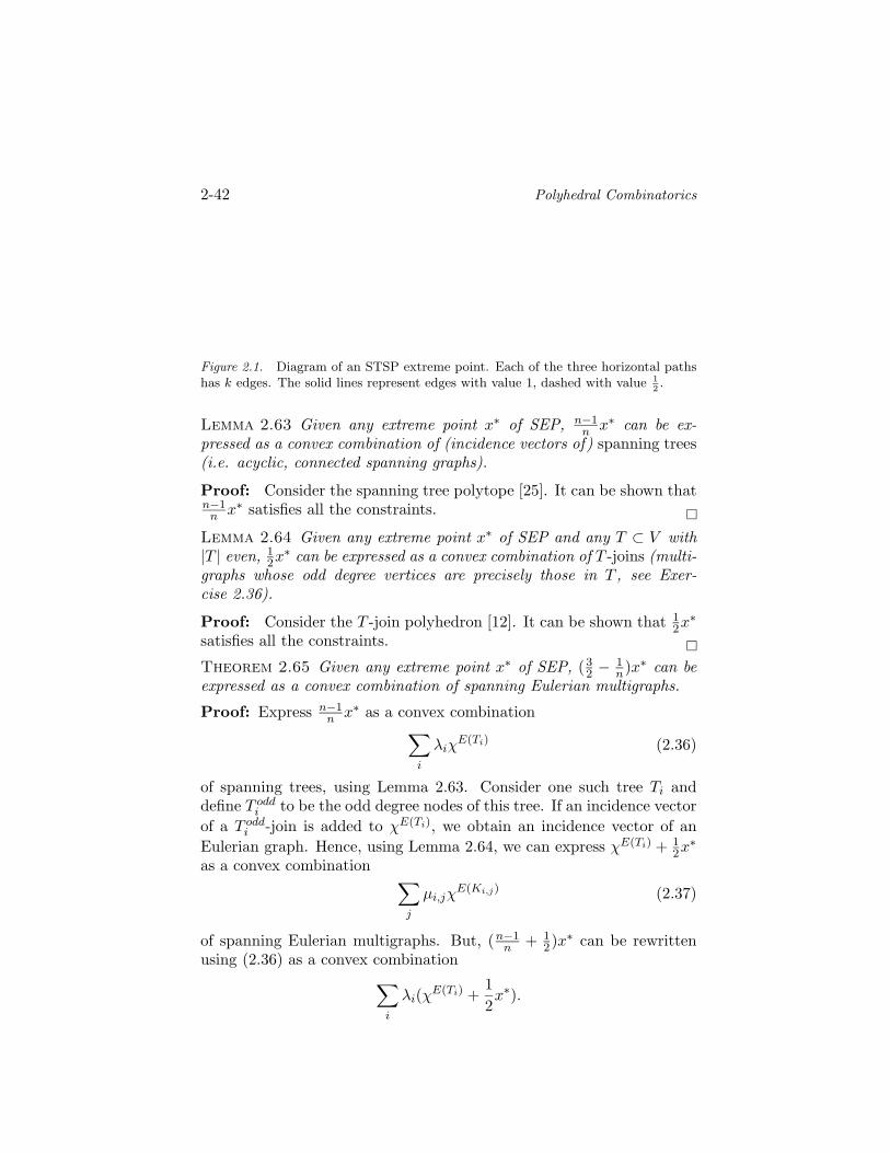
2-42 Polyhedral Combinatorics
Figure 2.1. Diagram of an STSP extreme point. Each of the three horizontal pathshas k edges. The solid lines represent edges with value 1, dashed with value 1
2.
Lemma 2.63 Given any extreme point x∗ of SEP, n−1n x∗ can be ex-
pressed as a convex combination of (incidence vectors of) spanning trees(i.e. acyclic, connected spanning graphs).
Proof: Consider the spanning tree polytope [25]. It can be shown thatn−1n x∗ satisfies all the constraints.
Lemma 2.64 Given any extreme point x∗ of SEP and any T ⊂ V with|T | even, 1
2x∗ can be expressed as a convex combination of T -joins (multi-
graphs whose odd degree vertices are precisely those in T , see Exer-cise 2.36).
Proof: Consider the T -join polyhedron [12]. It can be shown that 12x∗
satisfies all the constraints.
Theorem 2.65 Given any extreme point x∗ of SEP, (32 −
1n)x∗ can be
expressed as a convex combination of spanning Eulerian multigraphs.
Proof: Express n−1n x∗ as a convex combination∑
i
λiχE(Ti) (2.36)
of spanning trees, using Lemma 2.63. Consider one such tree Ti anddefine T oddi to be the odd degree nodes of this tree. If an incidence vectorof a T oddi -join is added to χE(Ti), we obtain an incidence vector of anEulerian graph. Hence, using Lemma 2.64, we can express χE(Ti) + 1
2x∗
as a convex combination ∑j
µi,jχE(Ki,j) (2.37)
of spanning Eulerian multigraphs. But, (n−1n + 1
2)x∗ can be rewrittenusing (2.36) as a convex combination∑
i
λi(χE(Ti) +12x∗).
Approximation Algorithms, Integrality Gaps and Polyhedral Embeddings 2-43
Therefore, (n−1n + 1
2)x∗ can be expressed as the convex combination∑i,j
λiµi,jχE(Ki,j)
of spanning Eulerian multigraphs by using (2.37), as required.
Corollary 2.66 The integrality gap of metric STSP is at most 3/2.
2.7.3 Half-integralityThe linear relaxation (2.35) of vertex cover in fact satisfies a strong,
very interesting property.
Theorem 2.67 [30] Every extreme point of the polyhedron defined bythe LP (2.35) has coordinates that all belong to {0, 1/2, 1}, that is, thepolyhedron is half-integral.
Proof: Let x∗ be an optimal solution to the LP (2.35) and define
U−1 = {v ∈ V | 0 < x∗v < 1/2},U1 = {v ∈ V | 1/2 < x∗v < 1}.
Then modify the values of x∗v for those v contained in either U−1 or U1:define y1
v = x∗v + kε and y2v = x∗v − kε if v ∈ Uk, for k ∈ {−1, 1}. Define
y1v = y2
v = xv for v 6∈ U−1 ∪ U1. Then x∗ = (y1 + y2)/2. If either U−1 orU1 is nonempty, ε may be chosen small enough that both y1 and y2 arefeasible, and thus U−1 = U1 = ∅ for an extreme point x∗.
Half-integrality is common in combinatorial optimization. We giveanother example in Section 2.7.5 and refer the reader to Hochbaum’ssurvey [16] for additional results.
2.7.4 Rounding ReductionsOccasionally, approximation algorithms may be composed by reduc-
tions that preserve approximation guarantees. For example, suppose wecan transform an instance IA of problem A to an instance IB of prob-lem B so that there is a one-to-one correspondence between solutionsof IA and those of IB such that if sA is a solution to IA and sB thecorresponding solution to IB, their costs satisfy αc(sA) ≥ c(sB). Thena β-approximation algorithm for B implies an αβ approximation algo-rithm for A.
In Section 2.7.5 we present such a reduction that uses linear relax-ations and rounding. The problems involved are the weighted edge-dominating set (EDS) and edge-cover (EC). The algorithm starts with
2-44 Polyhedral Combinatorics
an optimal solution of a relaxation of EDS and multiplies it by 2. Theresulting point can be interpreted as a solution to a relaxation of EC,and after multiplication by 4/3 expressed (after reducing the values ofsome of the variables) as a convex combination of integral solutions.
Other similar results exist [2, 22]. The integrality gap or the approxi-mation guarantee is sometimes the product of those achieved by the in-termediate steps (Section 2.7.5) and sometimes the sum (Section 2.7.2).Even better results are sometimes possible with careful analysis [4].
2.7.5 Weighted edge-dominating setsGiven a graph G = (V,E) with a cost function c : E → R+ defined on
the edge set, an edge-dominating set of G is any subset F ⊆ E of edgessuch that for every e ∈ E, at least one edge adjacent to e is containedin F . The cost of an edge-dominating set is defined as the sum of thecosts of its edges. An optimal solution to the edge-dominating set (EDS)instance defined by G is then a minimum-cost edge-dominating set.
For edges e, f ∈ E, write e ∼ f if e and f are adjacent. A simplelinear relaxation for EDS is as follows.
minimize∑
e∈E cexesubject to ∑
f∼e xf ≥ 1 ∀e ∈ E0 ≤ x ≤ 1
(2.38)
Let x∗ be an optimal solution to (2.38). Then for each edge uv ∈ E,
max{2x∗(δ(u)), 2x∗(δ(v))} ≥ 1 + x∗uv.
For each edge e ∈ E, let ve be the endpoint that achieves the maximumabove. Then let U = {ve | e ∈ E}, and ye = min{2x∗e, 1} for all e ∈ E.The point y is now an element of the polyhedron
0 ≤ ye ≤ 1 ∀e ∈ Ey(δ(v)) ≥ 1 ∀v ∈ U. (2.39)
An important observation is that any integral solution to (2.39) is also anedge-dominating set for G. We shall prove that an extreme point optimalsolution to (2.39) can be efficiently rounded to an edge-dominating setwhile increasing the cost by a factor at most 4/3, implying an 8/3-approximation algorithm (and integrality gap) for EDS.
Theorem 2.68 Let y∗ be an extreme point of the polyhedron (2.39).Then y∗ is half-integral and the edges of value 1/2 induce disjoint oddcycles in G.
Approximation Algorithms, Integrality Gaps and Polyhedral Embeddings 2-45
The proof of Theorem 2.68 is longer, but based on the same ideas asthat of Theorem 2.67 (half-integrality of vertex cover).
A final fact needed to justify the performance guarantee:
Lemma 2.69 Let C be an odd cycle of edges with value 1/2. Let yC de-note the vector of fractional edge-values of C. Then (4/3)yC dominatesa convex combination of edge-covers of C.
Proof: Let C = (VC , EC), where VC = {v1, . . . , vk} and EC ={v1v2, v2v3, . . . , vkv1}. Define integral edge-covers D1, . . . , Dk as follows.For each i, Di will have (k+ 1)/2 edges. For i < k, let Di contain ei andei+1. Then add (k − 3)/2 edges to Di so that ei and ei+1 are the onlyadjacent pair of edges in Di. In Dk, the adjacent edges are ek and e1.
Let yi denote the incidence vector of Di. Then
y0 =1k
(y1 + y2 + · · ·+ yk)
is a convex combination of edge-covers, and y0i = (k + 1)/(2k) for all
i. Since 4/3 ≥ (k + 1)/k for all k ≥ 3 (and the shortest odd cycle is atriangle), it follows that (4/3)yC ≥ y0.
Note that, because the sum of coefficients in any convex combinationis 1, it follows that at least one of the edge-covers D1, . . . , Dk has costno more than 4/3 times the cost of yC .
Algorithm:
(1) Solve the LP-relaxation (2.38). Let xLP be an optimal solution.
(2) Let U = ∅. For each edge e = uv ∈ E, if xLP (δ(u)) ≥ 1/2, add uto U , otherwise add v to U .
(3) Solve the relaxed edge-cover linear program, where the constraintsy(δ(u)) ≥ 1 are included only for u ∈ U , and the objective functionis min
∑e∈E ceye. Find an optimal solution y∗ which is an extreme
point.
(4) Let D = {e ∈ E | y∗e = 1}. Find the least cost edge-cover of eachodd cycle in y∗, and add its edges to D.
(5) Output D.
Note that D is an edge-dominating set because the edge-covering con-straints for U require at least one endpoint of each edge in E to becovered (dominated) by an edge in D.
Theorem 2.70 The edge-dominating set D that the above algorithmoutputs has cost no more than 8/3 times the cost of an optimal edge-dominating set.
2-46 Polyhedral Combinatorics
Theorem 2.71 For any extreme point xLP of (2.38), (8/3)xLP domi-nates a convex combination of edge-dominating sets. Thus the integralitygap of the LP (2.38) is at most 8/3.
A more careful analysis shows that the integrality gap of the relax-ation (2.38) is in fact at most 2.1. In fact, the integrality gap is exactly2.1 [4]: consider the complete graph K5n on 5n vertices and partition itinto n disjoint copies of K5, named G1, . . . , Gn. Let ce = 1 for each edgee induced by some Gi, and ce = 11n for every other edge e. Now anyintegral edge-dominating set has cost at least 3n − 1, but on the otherhand assigning xe = 1/7 to all the edges of Gi for each i results in afeasible solution of cost 10n/7.
It is possible to strengthen the linear relaxation (2.38) by adding in-equalities for hypomatchable sets [32]. The integrality gap of the resultingrelaxation is 2, and an algorithm with approximation guarantee 2 fol-lows as well. Further improvements would imply improvements also forvertex cover, which is an outstanding open problem.
As a final remark, we note that the algorithm described above, aswell as many others based on the same paradigm, can actually be imple-mented without explicitly solving the initial LP relaxation, and insteadbased on (more efficient) algorithms for approximating the “intermediateproblem” (vertex cover).
AcknowledgmentThis chapter arose partially from notes for a course taught at theUniversity of New Mexico. Sandia is a multiprogram laboratoryoperated by Sandia Corporation, a Lockheed Martin Company, for theU.S. Department of Energy under Contract DE-AC04-94AL85000.
References
[1] E. Balas and M. Fischetti. Polyhedral theory for the asymmetric travelingsalesman problem. In The traveling salesman problem and its variations, pages117–168. Kluwer, 2002.
[2] D. Bienstock, M. Goemans, D. Simchi-Levi, and David Williamson. A note onthe prize-collecting traveling salesman problem. Mathematical Programming,Series A, 59(3):413–420, 1993.
[3] S. Boyd and R. D. Carr. A new bound for the radio between the 2-matchingproblem and its linear relaxation. Mathematical Programming, Series A,86(3):499–514, 1999.
[4] R. D. Carr, T. Fujito, G. Konjevod, and O. Parekh. A 2 110
approximationalgorithm for a generalization of the weighted edge-dominating set problem.Journal of Combinatorial Optimization, 5:317–326, 2001.
References 2-47
[5] R. D. Carr and G. Lancia. Compact vs. exponential-size LP relaxations. Oper-ations Research Letters, 30(1):57–65, 2002.
[6] R. D. Carr and S. Vempala. Towards a 4/3-approximation for the asymmetrictraveling salesman problem. In Proceedings of the 11th Annual ACM-SIAMSymposium on Discrete Algorithms, pages 116–125, 2000.
[7] V. Chvatal. Linear programming. Freeman, 1983.
[8] S. de Vries, M. E. Posner, and R. Vohra. Polyhedral properties of the K-medianproblem on a tree. No 1367 in Discussion Papers, Northwestern University,Center for Mathematical Studies in Economics and Management Science, 42pages, 2003.
[9] E. V. Denardo. Dynamic programming: theory and practice. Prentice-Hall, 1978.
[10] J. Edmonds. Optimum branchings. Journal of Research of the National Bureauof Standards, 71B:233–240, 1967.
[11] L. R. Ford and D. R. Fulkerson. Flows in Networks. Princeton University Press,Princeton, NJ, 1962.
[12] A. M. H. Gerards. Matching. In Network models, volume 7 of Handbooks inOperations Research, pages 135–224. Elsevier, 1995.
[13] M. Goemans. Worst-case comparison of valid inequalities for the TSP. Mathe-matical Programming, 69:335–349, 1995.
[14] M. Grotschel and L. Lovasz. Combinatorial optimization. In Handbook of com-binatorics, volume 2, pages 1541–1597. Elsevier, 1995.
[15] M. Grotschel, L. Lovasz, and A. Schrijver. Geometric Algorithms and Combi-natorial Optimization. Springer Verlag, 1988.
[16] D. S. Hochbaum. Approximating covering and packing problems: set cover, ver-tex cover, independent set, and related problems. In Approximation algorithmsfor NP-hard problems, pages 94–143. PWS, 1997.
[17] T. Ibaraki. Solvable classes of discrete dynamic programming. Journal of Math-ematical Analysis and Applications, 43:642–693, 1973.
[18] R. G. Jeroslow. On defining sets of vertices of the hypercube by linear inequal-ities. Discrete Mathematics, 11:119–124, 1975.
[19] M. Junger, G. Reinelt, and G. Rinaldi. The traveling salesman problem. InNetwork models, volume 7 of Handbooks in Operations Research, pages 225–329.Elsevier, 1995.
[20] V. Kaibel and M. Pfetsch. Some algorithmic problems in polytope theory. InAlgebra, Geometry and Software Systems, pages 23–47. Springer Verlag, 2003.arXiv:math.CO/0202204v1.
[21] R. M. Karp and M. Held. Finite state processes and dynamic programming.SIAM Journal of Applied Mathematics, 15:693–718, 1967.
[22] J. Konemann, G. Konjevod, O. Parekh, and A. Sinha. Improved approximationalgorithms for tour and tree covers. In Proceedings of APPROX 2000, volume1913 of Lecture Notes in Computer Science, pages 184–193, 2000.
[23] G. Konjevod, R. Ravi, and A. Srinivasan. Approximation algorithms for thecovering Steiner problem. Random Structures & Algorithms, 20:465–482, 2002.
[24] B. Korte and J. Vygen. Combinatorial optimization. Theory and algorithms.Springer Verlag, 2000.
2-48 Polyhedral Combinatorics
[25] T. L. Magnanti and L. A. Wolsey. Optimal trees. In Network models, volume 7of Handbooks in Operations Research, pages 503–615. Elsevier, 1995.
[26] R. K. Martin. Using separations algorithms to generate mixed integer modelreformulations. Operations Research Letters, 10(3):119–128, 1991.
[27] R. K. Martin, R. Rardin, and B. A. Campbell. Polyhedral characterizations ofdiscrete dynamic programming. Operations Research, 38(1):127–138, 1990.
[28] D. Naddef. Polyhedral theory and branch-and-cut algorithms for the symmet-ric TSP. In The traveling salesman problem and its variations, pages 29–116.Kluwer, 2002.
[29] G. Nemhauser and L. Wolsey. Integer and Combinatorial Optimization. Wiley,1988.
[30] G. L. Nemhauser and L. E. Trotter. Properties of vertex packing and indepen-dence system polyhedra. Mathematical Programming, 6:48–61, 1974.
[31] C. Papadimitriou. Computational Complexity. Addison-Wesley, 1994.
[32] O. Parekh. Edge-dominating and hypomatchable sets. In Proceedings of the13th Annual ACM-SIAM Symposium on Discrete Algorithms, pages 287–291,2002.
[33] W. R. Pulleyblank. Polyhedral combinatorics. In Optimization, volume 1 ofHandbooks in Operations Research, pages 371–446. Elsevier, 1989.
[34] W. R. Pulleyblank. Matchings and extensions. In Handbook of combinatorics,volume 1, pages 179–232. Elsevier, 1995.
[35] A. Schrijver. Theory of Linear and Integer Programming. Wiley, 1986.
[36] A. Schrijver. Polyhedral combinatorics. In Handbook of combinatorics, volume 2,pages 1649–1704. Elsevier, 1995.
[37] A. Schrijver. Combinatorial Optimization: Polyhedra and Efficiency. SpringerVerlag, 2003.
[38] D. B. Shmoys and D. P. Williamson. Analyzing the Held-Karp TSP bound: amonotonicity property with application. Information Processing Letters, 35:281–285, 1990.
[39] A. Tamir. An O(pn2) algorithm for the p-median and related problems on treegraphs. Operations Research Letters, 19(2):59–64, 1996.
[40] T. Terlaky and S. Zhang. Pivot rules for linear programming: a survey on recenttheoretical developments. Annals of Operations Research, 46:203–233, 1993.
[41] V. V. Vazirani. Approximation algorithms. Springer Verlag, 2001.
[42] L. A. Wolsey. Heuristic analysis, linear programming and branch and bound.Mathematical Programming Study, 13:121–134, 1980.
[43] M. Yannakakis. Expressing combinatorial optimization problems by linear pro-grams. Journal of Computer and System Sciences, 43(3):441–466, 1991.
[44] G. Ziegler. Lectures on Polytopes. Springer, 1995.