13

CHAPTER 2

SEDIMENT TRANSPORT UNDER SIZE SELECTIVE CONDITIONS

2.1 INTRODUCTION

Transient processes in rivers occur at different spatial scales: i) the macro-scale, adequate

to understand the morphologic evolution of the river valley; ii) the meso-scale, appropriate to

study delimited river zones such as reaches subjected to, for instance, persistent aggradation

or degradation; iii) the micro-scale, the scale of the flow depth and of the bed forms and iv)

the grain-scale, the scale at which fluid-sediment interaction takes place, namely momentum

transfer from the fluid flow to the sediment grains at the bed and the collisional transfer of

momentum among sediment grains. The first three scales are classical in alluvial morphology

studies (Klaassen 1988) while the fourth is an evermore workable scale as the improvement

of measuring and computational techniques allow researchers to perform reliable

measurements and numerical simulations within it (cf. Nelson et al. 1995, Schmeeckle &

Nelson 2003).

The first objective of the present chapter is the development of a conceptual model based on

a set of differential equations that express the fundamental conservation principles in

unsteady open-channel flows with mobile beds composed of cohesionless poorly sorted

sediment. It is intended that the range of applicability of the ensuing model belongs to the

14

domain of the meso-scale problems. In other words, the conceptual model should be able to

describe the mechanics of sediment transport and associated morphologic impacts in

delimited river reaches.

In order to optimize the delicate compromise between solution quality, formal complexity and

computational cost, it is impossible to express all the phenomena through conservation

equations. The system of conservation laws is open, i.e., the number of unknowns is larger

than the number of conservation equations. Thus, it is necessary to specify much of the

relevant phenomena as closure equations.

The second objective of the present chapter is the development of closure equations that

account for the most relevant fluid-sediment interaction phenomena. These comprise energy

dissipation and sediment transport. The materialization of the later into semi-empirical

equations requires the specification of grain velocity and of hiding and protrusion effects.

The closure equations will be derived strictly within the grain-scale framework. The closure

sub-model will be applicable to flows where the macroscopic flow variables such as the

friction slope and the sediment discharge are a result from the integration of processes that

take place at the scale of the grain. For instance, it is intended that the sediment discharge

formula should be based on the quantification of the momentum transfer from the fluid flow to

the sediment grains, during shear-producing turbulent events. Therefore, micro-scale

phenomena will not be addressed in the theoretical and experimental work that is presented

in this chapter. In particular, bed-form induced flow resistance will not be studied nor any

other aspects pertaining bed form formation and destruction.

This restricts the domain of application of the conceptual model to gravel- and sand-bed

rivers featuring low Froude numbers. Upper plane bed flow would also be amenable to a

grain-scale description. Such study is left out of the scope of this chapter and is undertaken

in Chapter 3.

The proposed conceptual model is one-dimensional. The reason for not including other space

dimensions is related to the nature of the work program. The straightforward way to include

grain-scale effects is by means of semi-empirical formulæ. These are developed in

controlled laboratorial experiments, that express, in terms of micro-variables like flow depth,

mean velocity shear stress or bedload discharge, phenomena that ultimately depend on grain-

scale interactions. Thus, such semi-empirical formulæ are, ultimately, one-dimensional.

The best classic example is Einstein’s (1950) derivation of his bedload formula, based on the

mean step length of individual particles and on the pick up and rest probabilities of bed

particles. Such a formula can easily be generalised to a vectorial space, retaining the velocity

vector as a variable, and introduced in a two-dimensional model. Yet, it is still a one-

dimensional formula.

It is noted that considerable scientific investment has been made with the objective of

improving one-dimensional models. Because they may be regarded as a nursery of semi-

empirical closure sub-models, a great proportion of the relevant research is of

phenomenological nature (cf. Hirano 1971, Ashida & Michue 1971, Fernandez Luque & van

Beek 1976, Parker et al. 1982, Bell & Sutherland 1983, Parker 1990, Niño et al. 1994,

Armanini & di Silvio 1988, Armanini 1995, Hoey & Ferguson 1994, Toro Escobar et. al. 1996,

Nikora et al. 2001, Parker et al. 2003, among others). But it should be emphasised that there

15

are also abundant examples of investigation on the mathematical properties of the

conservation equations (Lyn 1987, Saiedi 1997, Cao et al. 2002, Lyn & Altinakar 2002), on

the numerical properties of the applicable discretization schemes (Preissmann, 1961, Lyn &

Goodwin 1987, Lai et al. 1994) and on the production of new benchmark data for some

problems (Belo 1992, §5 and 6, pp. 71 -128).

Vast applicability, low computational cost and conceptual simplicity are, thus, the main

reasons that justify the continuing scientific investment in the development of one-

dimensional models. In particular, the properties of the global structure of the model must be

known so that the contribution of the phenomenological closure sub-models is properly

isolated and understood. If the conservation structure of the model is well established, this

will allow for a proper understanding of the role of the closure equations.

A first step in this direction is achieved by understanding the prolegomena of one-

dimensional modelling of morphologic problems. The first attempts to model the unsteady

open-channel flows with mobile beds avoided the explicit description of vertical fluxes of

sediment between the flow and the bed. Because of computational constraints, these fluxes

would be included by means of a sediment discharge formula parameterized to flow variables

such as the mean flow velocity, the flow depth or the shear stress. The result is sufficiently

good if the time scales of sediment phenomena are sufficiently larger than those of the

hydrodynamic phenomena (Klaassen 1988).

De Vries (1965) model, applicable to unsteady open-channel flows with mobile beds, is the

archetypal example of these early modelling efforts. The conservation equations comprehend

the Saint-Venant equations for clear water and a sediment mass conservation equation, or

Exner-Polya equation, according to Yalin (1992), p. 24. The system can be written as

( ) ( ) 0t xh uh∂ + ∂ = (2.1)

( ) ( ) ( ) ( ) ( )( )wt x x x b bu u u g h g Y h∂ + ∂ + ∂ + ∂ = −τ ρ (2.2)

( ) ( )(1 ) 0t b x sp Y q− ∂ + ∂ = (2.3)

where the symbols refer to the water depth, h, the depth-averaged flow velocity, u, the bed

elevation, Yb, the bed shear stress, τb, the water density, ( )wρ , the sediment discharge, qs, the

porosity of the bed, p, and the acceleration of gravity, g. The system is closed by the closure

equations that specify the flow resistance and the equilibrium sediment transport rate.

Without loss of generality, it can be assumed that the closure models must specify τb and qs

as a functions of the dependent variables h and u and of a number of parameters concerning

the fluid (mainly viscosity and density) and the sediment (mainly density, descriptors of size

distribution but also coefficient of restitution and granular temperature as seen in Chapter 3).

If the Froude number of the flow is small, one has

( )( ) ( ), ; , , , , ,w gb b s gh u d gτ = τ μ ρ ρ σ (2.4)

( )( ) ( ), ; , , , , ,w gs s s gq q h u d g= μ ρ ρ σ (2.5)

where μ is the fluid viscosity, ( )gρ the density of the sediment grains, ds is a representative

diameter of the sediment mixture, for instance the mean diameter, and σg is a representative

second moment of the grain size distribution or a related parameter, for instance the

16

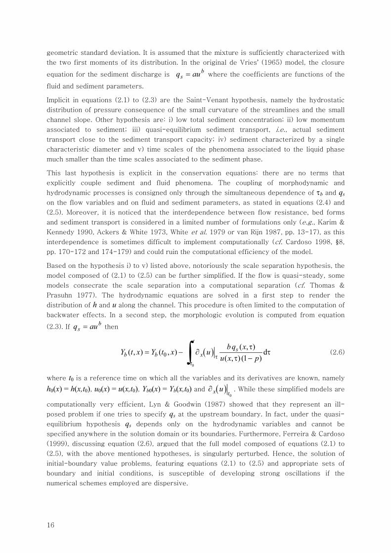
geometric standard deviation. It is assumed that the mixture is sufficiently characterized with

the two first moments of its distribution. In the original de Vries’ (1965) model, the closure

equation for the sediment discharge is b

s auq = where the coefficients are functions of the

fluid and sediment parameters.

Implicit in equations (2.1) to (2.3) are the Saint-Venant hypothesis, namely the hydrostatic

distribution of pressure consequence of the small curvature of the streamlines and the small

channel slope. Other hypothesis are: i) low total sediment concentration; ii) low momentum

associated to sediment; iii) quasi-equilibrium sediment transport, i.e., actual sediment

transport close to the sediment transport capacity; iv) sediment characterized by a single

characteristic diameter and v) time scales of the phenomena associated to the liquid phase

much smaller than the time scales associated to the sediment phase.

This last hypothesis is explicit in the conservation equations: there are no terms that

explicitly couple sediment and fluid phenomena. The coupling of morphodynamic and

hydrodynamic processes is consigned only through the simultaneous dependence of τb and qs

on the flow variables and on fluid and sediment parameters, as stated in equations (2.4) and

(2.5). Moreover, it is noticed that the interdependence between flow resistance, bed forms

and sediment transport is considered in a limited number of formulations only (e.g., Karim &

Kennedy 1990, Ackers & White 1973, White et al. 1979 or van Rijn 1987, pp. 13-17), as this

interdependence is sometimes difficult to implement computationally (cf. Cardoso 1998, §8,

pp. 170-172 and 174-179) and could ruin the computational efficiency of the model.

Based on the hypothesis i) to v) listed above, notoriously the scale separation hypothesis, the

model composed of (2.1) to (2.5) can be further simplified. If the flow is quasi-steady, some

models consecrate the scale separation into a computational separation (cf. Thomas &

Prasuhn 1977). The hydrodynamic equations are solved in a first step to render the

distribution of h and u along the channel. This procedure is often limited to the computation of

backwater effects. In a second step, the morphologic evolution is computed from equation

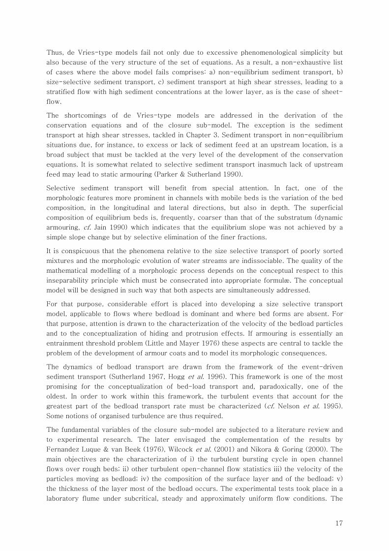
(2.3). If b

s auq = then

( )0

0( , )

( , ) ( , ) d( , ) (1 )

ts

b b xt

b q xY t x Y t x u

u x pτ

τ= − ∂ τ

τ −∫ (2.6)

where t0 is a reference time on which all the variables and its derivatives are known, namely

h0(x) = h(x,t0), u0(x) = u(x,t0), Yb0(x) = Yb(x,t0) and ( )0

x tu∂ . While these simplified models are

computationally very efficient, Lyn & Goodwin (1987) showed that they represent an ill-

posed problem if one tries to specify qs at the upstream boundary. In fact, under the quasi-

equilibrium hypothesis qs depends only on the hydrodynamic variables and cannot be

specified anywhere in the solution domain or its boundaries. Furthermore, Ferreira & Cardoso

(1999), discussing equation (2.6), argued that the full model composed of equations (2.1) to

(2.5), with the above mentioned hypotheses, is singularly perturbed. Hence, the solution of

initial-boundary value problems, featuring equations (2.1) to (2.5) and appropriate sets of

boundary and initial conditions, is susceptible of developing strong oscillations if the

numerical schemes employed are dispersive.

17

Thus, de Vries-type models fail not only due to excessive phenomenological simplicity but

also because of the very structure of the set of equations. As a result, a non-exhaustive list

of cases where the above model fails comprises: a) non-equilibrium sediment transport, b)

size-selective sediment transport, c) sediment transport at high shear stresses, leading to a

stratified flow with high sediment concentrations at the lower layer, as is the case of sheet-

flow.

The shortcomings of de Vries-type models are addressed in the derivation of the

conservation equations and of the closure sub-model. The exception is the sediment

transport at high shear stresses, tackled in Chapter 3. Sediment transport in non-equilibrium

situations due, for instance, to excess or lack of sediment feed at an upstream location, is a

broad subject that must be tackled at the very level of the development of the conservation

equations. It is somewhat related to selective sediment transport inasmuch lack of upstream

feed may lead to static armouring (Parker & Sutherland 1990).

Selective sediment transport will benefit from special attention. In fact, one of the

morphologic features more prominent in channels with mobile beds is the variation of the bed

composition, in the longitudinal and lateral directions, but also in depth. The superficial

composition of equilibrium beds is, frequently, coarser than that of the substratum (dynamic

armouring, cf. Jain 1990) which indicates that the equilibrium slope was not achieved by a

simple slope change but by selective elimination of the finer fractions.

It is conspicuous that the phenomena relative to the size selective transport of poorly sorted

mixtures and the morphologic evolution of water streams are indissociable. The quality of the

mathematical modelling of a morphologic process depends on the conceptual respect to this

inseparability principle which must be consecrated into appropriate formulæ. The conceptual

model will be designed in such way that both aspects are simultaneously addressed.

For that purpose, considerable effort is placed into developing a size selective transport

model, applicable to flows where bedload is dominant and where bed forms are absent. For

that purpose, attention is drawn to the characterization of the velocity of the bedload particles

and to the conceptualization of hiding and protrusion effects. If armouring is essentially an

entrainment threshold problem (Little and Mayer 1976) these aspects are central to tackle the

problem of the development of armour coats and to model its morphologic consequences.

The dynamics of bedload transport are drawn from the framework of the event-driven

sediment transport (Sutherland 1967, Hogg et al. 1996). This framework is one of the most

promising for the conceptualization of bed-load transport and, paradoxically, one of the

oldest. In order to work within this framework, the turbulent events that account for the

greatest part of the bedload transport rate must be characterized (cf. Nelson et al. 1995).

Some notions of organised turbulence are thus required.

The fundamental variables of the closure sub-model are subjected to a literature review and

to experimental research. The later envisaged the complementation of the results by

Fernandez Luque & van Beek (1976), Wilcock et al. (2001) and Nikora & Goring (2000). The

main objectives are the characterization of i) the turbulent bursting cycle in open channel

flows over rough beds; ii) other turbulent open-channel flow statistics iii) the velocity of the

particles moving as bedload; iv) the composition of the surface layer and of the bedload; v)

the thickness of the layer most of the bedload occurs. The experimental tests took place in a

laboratory flume under subcritical, steady and approximately uniform flow conditions. The

18

bed was permeable and composed of cohesionless natural sediment, transported exclusively

as bed-load. No appreciable bed forms were registered.

The prosecution of the objectives outlined above shapes the structure of the present chapter.

Its first sub-chapter, §2.2, is dedicated to the derivation of the conservation equations of the

conceptual model. For this purpose, a control volume analysis similar to that of Armanini & di

Silvio (1988) is privileged. The physical system is first described, a task that is followed by

the derivation of the differential equations that express the conservation of mass and

momentum of both the water and the sediment constituents. This is followed by a discussion

of the less well-known terms of these equations. It is aimed at the elimination of algebraically

less important terms in order to simplify the solution procedure. At the end of §2.2 there is a

summary of the governing equations written in suitable forms for numerical discretization.

The derivation of the closure equations is partially based in experimental evidence produced

for that purpose. Before deriving the closure equations, the characterization of the

experimental tests, namely the installations, the equipment and the procedures, is performed

in §2.3.1 and §2.3.2. The presentation of the experimental results and its discussion is

presented in §2.4. Special emphasis is given to i) the characterization of the velocity profiles

and other mean quantities, ii) the description of the bursting cycle in open-channel turbulent

flows over rough fixed and mobile beds, iii) the quantification of the velocity of the sediment

particles, iv) the quantification of the thickness of the most relevant layers and v) the

evaluation of the total and fractional bedload rates. Annex 2.4 is invoked in a sub-chapter; it

describes the development of a particle tracking algorithm that allows for the computation of

the statistics of the velocity of the particles transported as bedload.

The derivation of an event-driven bedload formula for the prediction of size-selective

sediment transport is undertaken in §2.4.7. It is based on a literature review and uses the

results of the experimental work. Hiding and protrusion effects are explicitly addressed by

means of a probabilistic analysis of the entrained volumes and formula calibration.

The chapter is ended by §2.5, a synthesis of the main results and prospects for future work.

2.2 DERIVATION OF THE GOVERNING EQUATIONS

2.2.1 General description of the physical system

Researchers on the mathematical modelling of size selective sediment transport and

associated changes in bed texture and morphology have found in the work of Hirano (1971)

their landmark study. It is, to this day, one of the conceptually best supported approaches.

The concept of a mixing layer1, placed between the transport layer and the bed and endowed

with filter functions, has allowed for the organization of the empirical information about the

vertical sediment fluxes between the bed and the transport layer.

The equation of conservation of the mixing layer, in Hirano’s original formulation, is formally

distinct depending on the type of morphologic process. If the porosity is considered constant,

for deposition one has

1 Also known as exchange layer or active layer (cf. Armanini 1995).

19

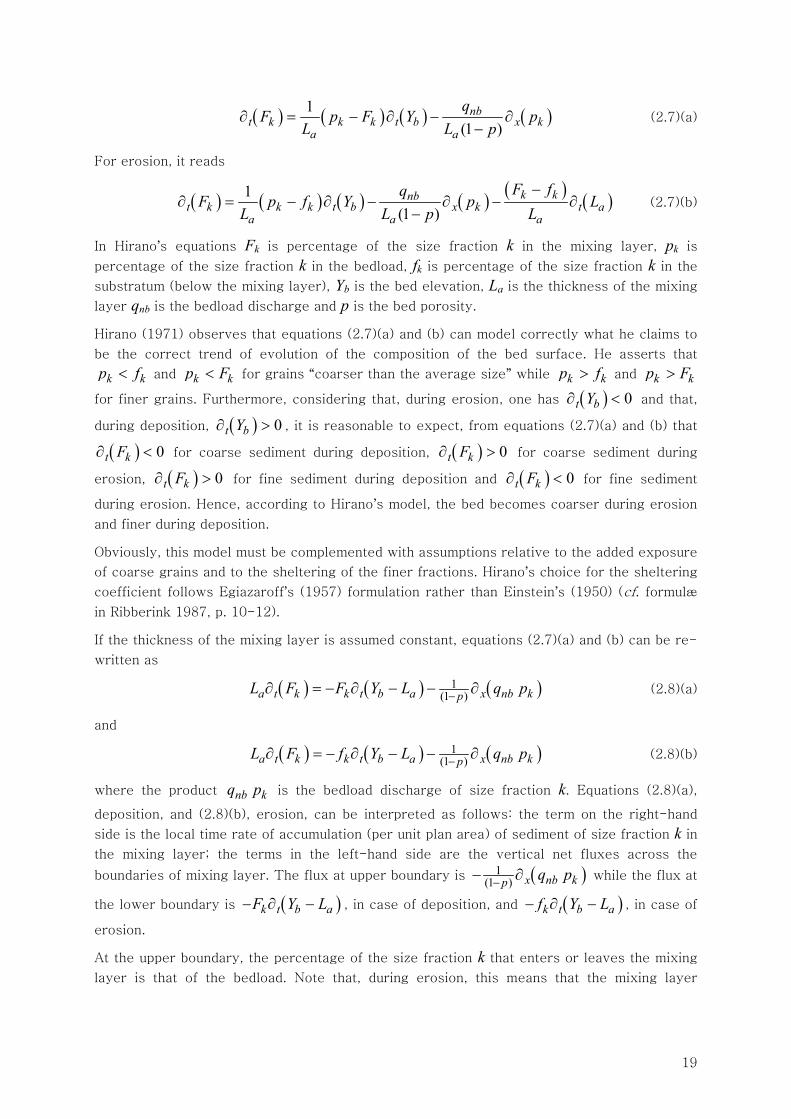
( ) ( ) ( ) ( )1(1 )

nbt k k k t b x k

a a

qF p F Y p

L L p∂ = − ∂ − ∂

− (2.7)(a)

For erosion, it reads

( ) ( ) ( ) ( ) ( ) ( )1(1 )

k knbt k k k t b x k t a

a a a

F fqF p f Y p L

L L p L−

∂ = − ∂ − ∂ − ∂−

(2.7)(b)

In Hirano’s equations Fk is percentage of the size fraction k in the mixing layer, pk is

percentage of the size fraction k in the bedload, fk is percentage of the size fraction k in the

substratum (below the mixing layer), Yb is the bed elevation, La is the thickness of the mixing

layer qnb is the bedload discharge and p is the bed porosity.

Hirano (1971) observes that equations (2.7)(a) and (b) can model correctly what he claims to

be the correct trend of evolution of the composition of the bed surface. He asserts that

k kp f< and k kp F< for grains “coarser than the average size” while k kp f> and k kp F>

for finer grains. Furthermore, considering that, during erosion, one has ( ) 0t bY∂ < and that,

during deposition, ( ) 0t bY∂ > , it is reasonable to expect, from equations (2.7)(a) and (b) that

( ) 0t kF∂ < for coarse sediment during deposition, ( ) 0t kF∂ > for coarse sediment during

erosion, ( ) 0t kF∂ > for fine sediment during deposition and ( ) 0t kF∂ < for fine sediment

during erosion. Hence, according to Hirano’s model, the bed becomes coarser during erosion

and finer during deposition.

Obviously, this model must be complemented with assumptions relative to the added exposure

of coarse grains and to the sheltering of the finer fractions. Hirano’s choice for the sheltering

coefficient follows Egiazaroff’s (1957) formulation rather than Einstein’s (1950) (cf. formulæ

in Ribberink 1987, p. 10-12).

If the thickness of the mixing layer is assumed constant, equations (2.7)(a) and (b) can be re-

written as

( ) ( ) ( )1(1 )a t k k t b a x nb kpL F F Y L q p−∂ = − ∂ − − ∂ (2.8)(a)

and

( ) ( ) ( )1(1 )a t k k t b a x nb kpL F f Y L q p−∂ = − ∂ − − ∂ (2.8)(b)

where the product nb kq p is the bedload discharge of size fraction k. Equations (2.8)(a),

deposition, and (2.8)(b), erosion, can be interpreted as follows: the term on the right-hand

side is the local time rate of accumulation (per unit plan area) of sediment of size fraction k in

the mixing layer; the terms in the left-hand side are the vertical net fluxes across the

boundaries of mixing layer. The flux at upper boundary is ( )1(1 ) x nb kp q p−− ∂ while the flux at

the lower boundary is ( )k t b aF Y L− ∂ − , in case of deposition, and ( )k t b af Y L− ∂ − , in case of

erosion.

At the upper boundary, the percentage of the size fraction k that enters or leaves the mixing

layer is that of the bedload. Note that, during erosion, this means that the mixing layer

20

controls the composition of the bedload. During deposition, it is implicit that the mixing layer

receives sediment with the composition of the bedload.

During deposition the mixing layer is displaced upwards. It is implicit in Hirano’s model that

the percentage of the size fraction k at the interface between the mixing layer and the

substratum is equal to that of the mixing layer itself. Thus, Hirano assumed that, as it moves

upwards, the mixing layer leaves behind its own composition. During erosion, it is implicit in

Hirano’s model that the percentage of the size fraction k at the interface between the mixing

layer and the substratum is equal to that of the substratum. This is equivalent to assuming

that, as the mixing moves downwards, the mixing layer incorporates sediment from the

substratum.

Hirano’s model have been generalized and modified over the past three decades. One of its

weak points, the assumptions regarding sediment composition at the boundaries of the mixing

layer, have been challenged and refined. Further investigation on vertical sediment exchange

(Ribberink 1987, §2, 3 and 4, pp. 7-72, Armanini & di Silvio 1988, Rahuel et al. 1989, di Silvio

1991, Hoey & Ferguson 1994, Toro-Escobar et al. 1996 and Cui et al. 1996) helped to

establish a paradigm, which, in this text, will be known as the multiple layer approach.

Despite this intensive research effort, the morphologic response of a gravel bed or a poorly

sorted sand bed water stream, given a number of initial and boundary conditions, is still

difficult to predict. This fact is due not so much to the conceptual formulation of the problem,

which, in its one-dimensional version, is elaborated and sophisticated enough, but rather to

the poor knowledge of some of the several parameters that stem, precisely, from the intended

sophistication.

Armanini (1995) objected to some of the theoretical assumptions of the multiple layer

modelling, namely the assumption that complete and instantaneous mixing of all grain sizes

occurs in the so-called mixing layer. He also considered that the absence of a vertical flux

between the mixing layer and the substratum, other than that provided by the vertical

displacement of the mixing layer, is a fault of multi-layer modelling.

This author proposed a different approach. The bed was sought to be a continuum medium

and the vertical sediment fluxes would be modelled as obeying to a Boussinesq diffusive

model. This approach gives rise to what can be called diffusive models, for which the

percentage of the size fraction k in the bed is given by

( ) ( )( )* *t k z z z kF F∂ = ∂ ε ∂ (2.9)

where εz is a diffusion coefficient, z stands for the vertical axis whose zero is at the bed

elevation and whose positive values are below the bed and * *( )k kF F z= is the percentage of

size-fraction k at a given depth, z, below the bed. The equation of conservation of size

fraction k transported near the bed includes the vertical flux

( )*0bY z k

zF

=−ε ∂

where bYε is a diffusion coefficient at the bed surface. Armanini, op. cit., provides a semi-

empirical expression relating bYε and εz. Furthermore, Armanini, op. cit., shows that the

equation of conservation of the mass of size fraction k in the mixing layer can be retrieved by

21

means of and upwind discretization of (2.9), introducing the equation of conservation of the

size fraction k in the bedload layer and neglecting a diffusive flux at the boundary between

the mixing layer and substratum. In that case, kF would be the average value of *kF between

z = 0 and z = La.

Although not relying on a great number of parameters, the results of these models depend

strongly on the values of the diffusion coefficients, in the bed surface and within the bed, for

which there is virtually no experimental data. Furthermore, the fundamental technique, the

Boussinesq decomposition into mean and fluctuating values seems more appropriate in beds

that develop strong amplitude bed forms. As stated before, the general purpose of this

dissertation is the study of unsteady flows with mobile beds whose main phenomena depends

only on grain-scale interactions between the flow and sediment grains. The effects of bed

forms, including its influence on the composition of the bed surface and of the bedload, are

not reducible to grain-scale interactions. Hence, the conceptual model herein presented is

developed within the multiple layer paradigm.

A comparison between multiple layer and diffusive models can be seen in Ferreira & Cardoso

(1999). The evaluation of the merits of each model in that work is far from exhaustive. The

authors did not pursue the comparison further because of the lack of proper data to evaluate

the parameters of the diffusive model.

Understood as a family of techniques to build conceptual models, the multiple layer approach

enables the maintenance of the computational simplicity and tractability of the one

dimensional models while explicitly addressing vertical exchange processes. The concept of

layer is broadly understood as a constrained portion of the flow, whose dimensions are much

larger in the longitudinal direction than in the direction normal to the flow, where it is

believed that the fundamental quantities are approximately constant in a plane perpendicular

to the bed (uniform in the cross section), structurally invariant or self-similar. The boundaries

are virtual planes, e.g., time-averaged streamlines, developing along stream, through which

there are vertical fluxes of mass and momentum. The flow variables become depth-averaged

quantities, integrated over the layer thickness. For instance, the mean layer velocity and

concentration are

0

0

1 ( )dy h

ly

u uh

+Δ

= ξ ξΔ ∫ ,

0

0

1 ( ) ( )dy h

ll y

C u chu

+Δ

= ξ ξ ξΔ ∫ (2.10)(a)(b)

where Δh is the layer thickness, y0 the elevation of its lower boundary and ξ a dummy

variable that stands for the height above the bed.

It is notorious that the model composed of equations (2.1) to (2.5) does not comprise any

detailed phenomenological assumptions on how sediment is entrained from and deposited on

the bed. It neither contains references to sediment dynamics, namely where, near the bed or

in the water column, the sediment flow occurs and what are its driving forces. Net loss or net

accumulation of sediment in the bed, over the time, are a consequence of the behaviour of the

velocity gradient, as is clear from equation (2.6).

On the contrary, the model herein developed procures, using the multiple layer approach, a

delicate balance between the computational simplicity of one-dimensional models and the

22

phenomenological complexity of two-dimensional (in the vertical plane) models. A functional

description of the layers that were considered essential for the correct description of the

involved phenomena is undertaken next.

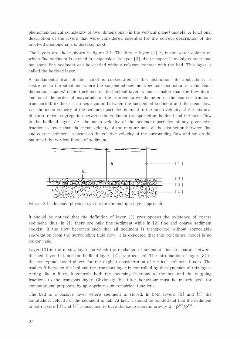
The layers are those shown in figure 2.1. The first - layer [1] -, is the water column on

which fine sediment is carried in suspension. In layer [2], the transport is mainly contact load

but some fine sediment can be carried without relevant contact with the bed. This layer is

called the bedload layer.

A fundamental trait of the model is consecrated in this distinction: its applicability is

restricted to the situations where the suspended-sediment/bedload distinction is valid. Such

distinction implies: i) the thickness of the bedload layer is much smaller than the flow depth

and is of the order of magnitude of the representative diameter of the coarser fractions

transported; ii) there is no segregation between the suspended sediment and the mean flow,

i.e., the mean velocity of the sediment particles is equal to the mean velocity of the mixture;

iii) there exists segregation between the sediment transported as bedload and the mean flow

in the bedload layer, i.e., the mean velocity of the sediment particles of any given size

fraction is lower than the mean velocity of the mixture and iv) the distinction between fine

and coarse sediment is based on the relative velocity of the surrounding flow and not on the

nature of the vertical fluxes of sediment.

FIGURE 2.1. Idealised physical system for the multiple layer approach

It should be noticed that the definition of layer [2] presupposes the existence of coarse

sediment; thus, in [1] there are only fine sediment while in [2] fine and coarse sediment

coexist. If the flow becomes such that all sediment is transported without appreciable

segregation from the surrounding fluid flow, it is expected that this conceptual model is no

longer valid.

Layer [3] is the mixing layer, on which the exchange of sediment, fine or coarse, between

the bed, layer [4], and the bedload layer, [2], is processed. The introduction of layer [3] in

the conceptual model allows for the explicit consideration of vertical sediment fluxes. The

trade-off between the bed and the transport layer is controlled by the dynamics of this layer.

Acting like a filter, it controls both the incoming fractions to the bed and the outgoing

fractions to the transport layer. Obviously this filter behaviour must be materialized, for

computational purposes, by appropriate semi-empirical functions.

The bed is a passive layer where sediment is stored. In both layers [3] and [4] the

longitudinal velocity of the sediment is null. At last, it should be pointed out that the sediment

in both layers [3] and [4] is assumed to have the same specific gravity ( ) ( )g ws = ρ ρ .

[ 4 ]

[ 1 ]

[ 2 ]

[ 3 ]

hb h

Yb

23

In the next sub-chapters, mass and momentum conservation equations will be derived for

each of the layers identified in figure 2.1. Closure equations will then be required to specify

some of the most relevant physical phenomena occurring in and between layers. In particular,

the thickness of the layers, the equilibrium sediment concentrations, the shear stress profiles

and the velocity profiles must be characterized. The important issues about hiding (or

sheltering, in Hirano 1971) and protrusion (or exposure) will also be addressed.

2.2.2 Mass and momentum equations

2.2.2.1 Introductory remarks

The equations of conservation of mass and momentum for each layer shown in figure 2.1, p.

22, are derived next. The physical system is composed of sediment and fluid constituents.

While the fluid is generally modelled as a continuum (Atkin & Craine 1970) even if laden with

fine sediment, coarse sediment moving as bedload is difficult to conceptualize as so. Yet, the

only practical way to model large numbers of moving particles is precisely to model the fluid-

sediment mixture as a continuum. Early modelling attempts would either model the entire flow

depth as a continuum or simply ignore the dynamic effects of the added density by assigning

an infinitely small thickness to the bedload layer (de Vries 1965).

The multiple layer approach followed in this work attempts a compromise between the

sophistication of two dimensional vertical flow descriptions and the tractability of the one

dimensional description. It follows that over the flow depth the density is not constant as in

the early models, but piecewise constant. Each layer is described as a continuum but the

existence of four layers, with different densities, allows for a better description of the

dynamics of the system.

In the following sections, continuum equations will be derived for the discrete fluid-sediment

system organized in the layers shown in figure 2.1, p. 22.

2.2.2.2 Depth- and flux-averaged quantities

The fundamental variables for each layer are summarized next.

Layer 1, suspended sediment layer:

• total mass, volume and momentum, (1)M ,

(1)∀ , (1)P ;

• mass and volume of sediment, (1)sM ,

(1)s∀ ;

• layer thickness, hw;

• velocity of the sediment constituent; at a given height above a datum, ( )( )su y , and

depth-averaged, usw;

• velocity of the water constituent; at a given height above a datum, ( ) ( )wu y , and depth-

averaged, uww;

• continuum layer velocity; at a given height above a datum, (1) ( )u y , and depth-

averaged, uw;

• concentration of suspended sediment; at a given height above a datum, (1)( )sC y , and

depth-averaged, (1)ˆsC ;

24

• flux-averaged concentration of suspended sediment, Cs;

• apparent sediment density; at a given height above a datum, (1) ( )s yρ , and depth-

averaged, (1)ˆ sρ ;

• apparent water density; at a given height above a datum, (1) ( )w yρ , and depth-averaged,

(1)ˆ wρ ;

• flux-averaged apparent density of suspended sediment, swρ

• flux-averaged apparent density of water, wwρ

• continuum layer density based on depth-averaged concentrations, (1)ρ ;

• continuum layer density based on flux-averaged concentrations, sρ ;

• suspended sediment discharge, qsw;

• water discharge, qww;

• total layer discharge, qw = hwuw = qsw + qww;

Layer 2, bedload layer:

• total mass and volume, (2)M ,

(2)∀ , (2)P ;

• mass and volume of fine sediment, (2)sM ,

(2)s∀ ;

• mass and volume of fine sediment, (2)cM ,

(2)c∀ ;

• layer thickness, hb;

• velocity of the fine sediment; at a given height above a datum, ( )( )su y , and depth-

averaged, usb;

• velocity of the coarse sediment; at a given height above a datum, ( )( )gu y , and depth-

averaged, ucb;

• velocity of the water constituent; at a given height above a datum, ( ) ( )wu y , and depth-

averaged, uwb;

• continuum layer velocity; at a given height above a datum, (2) ( )u y , and depth-

averaged, ub;

• concentration of fine sediment; at a given height above a datum, (2)( )sC y , and depth

averaged, (2)ˆsC ;

• concentration of coarse sediment; at a given height above a datum, (2)( )cC y , and depth

averaged, (2)ˆcC ;

• total concentration of sediment; at a given height above a datum, (2)( )C y , and depth

averaged, (2)C ;

• flux-averaged concentration of fine sediment, Csb;

25

• flux-averaged concentration of coarse sediment, Ccb;

• total flux-averaged concentration in the layer, Cb;

• apparent density of fine sediment; at a given height above a datum, (2) ( )s yρ , and

depth-averaged, (2)ˆ sρ ;

• apparent density of coarse sediment; at a given height above a datum, (2) ( )c yρ , and

depth-averaged, (2)ˆ cρ ;

• apparent depth-averaged sediment density, (2)ˆ nbρ ;

• apparent depth-averaged water density, (2)ˆ wbρ ;

• continuum layer density based on depth-averaged concentrations, (2)ρ ;

• continuum layer density based on flux-averaged concentrations, bρ ;

• fine sediment discharge, qsb;

• coarse sediment discharge, qcb;

• total sediment discharge in the layer, qnb = qsb + qcb;

• water discharge, qwb;

• total layer discharge, qb = hbub = qsb + qcb + qwb.

Flow depth, Layers 1 and 2:

• flow depth, h;

• depth-average mean flow velocity, u;

• total flux-averaged sediment concentration, C;

• continuum flux-averaged flow density, mρ ;

• sediment discharge, qs = qsw + qnb = qsw + qsb + qcb;

• total discharge, q = uh = qw + qb = qsw + qww + qsb + qcb + qwb.

Layers 3, mixing layer:

• mass and volume of sediment, (3)sM ,

(3)s∀ ;

• layer thickness, La;

• sediment concentration, reciprocal of porosity, Cbed = (1 – p);

• continuum layer density, bedρ .

Layer 4, substratum or undisturbed bed:

• mass and volume of sediment, (4)sM ,

(4)s∀ ;

• sediment concentration, reciprocal of porosity, Cbed = (1 – p).

• continuum layer density, bedρ .

26

The task of determining each of these variables will be undertaken next. The upper layer,

Layer 1, is characterised by transporting water and fine sediment. Leaving aside, for now,

considerations about the shape of the time-averaged velocity profile, u(y), the depth-

averaged flow velocity can be obtained from (2.10). For this particular layer it is

1 ( )d

b

h

ww h

u uh

= ξ ξ∫

where w bh h h= − . One of the hypothesis cited in §2.2.1 is that suspended sediment is

transported with a mean velocity close to that of the surrounding water flow. Thus,

sw ww wu u u≈ ≈ .

The depth-averaged volumetric concentration of fine sediment, designated Csw in Layer 1, can

be computed from

(1)(1)

(1)ˆ s

sw sC C∀

= ≡∀

(2.11)

where (1)s∀ is the volume of suspended sediment in the total volume,

(1)∀ , and (1)ˆ

sC is the

depth-averaged volumetric2 sediment concentration. Concentration measurements based on

image analysis would provide the result of (2.11).

Alternatively, concentrations can be measured from the analysis of a sample collected from

the flow. Typically, a small but representative volume is taken from the system by collecting

the total discharge over a time interval. The concentrations thus obtained are called flux-

averaged concentrations. In Layer 1, one obtains

swsw

w

qC

q= (2.12)

where

2

2

1 ( , ) d d

l

lb

h

wh

ql

−

= ξ σ ξ σ∫ ∫ u ni

and where l is the width of the plane that defines the cross-section. In strict one-

dimensional flows, wq is simply

2 In this text, all depth-average concentrations are volumetric concentrations. Massic concentrations for

layer n, ( )ˆ nsm , are defined as

( )( )

( ) ( )

( ) ( )( )

( ) ( )( ) ( )ˆ

g

g w

n nn s s

s n nn ns s

Mm

Mρ ∀

≡ =ρ ∀ + ρ ∀ −∀

where ( )nsM is the mass of sediment in layer n and

( )nM is the total mass in that layer. Hence, ( )ˆ nsm

can be retrieved from the volumetric concentration by

( )

( )( )

( )

ˆˆ

ˆ1 1

nn s

s ns

sCm

s C=

+ −

27

( )db

h

w w wh

q u h u= ξ ξ =∫ (2.13)

In Layer 1, equations (2.12) and (2.11) are equivalent. Yet, while (2.12) is generally easy to

determine in the laboratory or in the field, (2.11) is not generally easy to compute.

Depth-averaged and flux-averaged conceptions of concentration are equivalent if there is no

segregation between the transported size fractions and the water flow, i.e., if the time-

averaged velocity of the sediment is equal to the time averaged flow velocity at any depth. To

verify this claim, it should be noticed that the discharge of fine sediment in Layer 1 can be

given by

( )1 ds

s

sw sql

Ω

= Ω∫ u ni ⇔

( )

0

1 dlim dd

s

s

sw stq

l tΔ →Ω

= Ω∫ x ni (2.14)

where ( )su is the velocity of the suspended particles,

( )d sx is the excursion length of the

suspended sediment particles during dt and dΩs is the elemental area occupied by the

sediment particles on each element of a plane normal to the bed. Two elementary volumes

can be defined:

( ) ( )(1)d d d d dw wx S∀ = Ω =x ni (2.15)(a)

and

( ) ( )(1)d d d d ds s

s s sx S∀ = Ω =x ni (2.15)(b)

where ( )d wx is the excursion length of a fluid element during dt, dΩ is the total area of the

plane normal to the bed, dS is the projection of dΩ in the plane simultaneously normal to

the bed and the flow direction and d sS is the projection of d sΩ in the plane simultaneously

normal to the bed and the flow direction. From (2.11), (1) (1) (1)ˆd ds sC∀ = ∀ and, from (2.15)(a) and

(b), the integral (2.14) becomes

( ) ( ) ( )(1) (1)

sd 0 d 0 d 0

1 d 1 d 1 dˆ ˆlim d lim d lim dd d d

s w w

sw s st t tS S S

xq C C Sl t l t B t→ → →

= Ω = Ω =∫ ∫ ∫x xn ni i

in which ( ) ( )d dw wx=x ni and where B is the channel width. A simple algebraic manipulation

renders

( ) ( ) ( )(1) ( ) (1)

( ) ( )d 0

1 d d 1ˆ ˆlim d dd d

s w ws

s ssw s stS S

x x uq C S u C SB t x B u→

⎛ ⎞ ⎛ ⎞= =⎜ ⎟ ⎜ ⎟⎝ ⎠ ⎝ ⎠∫ ∫

where ( ) ( )d dw wu x t= is the velocity of fluid elements. Since

(1)ˆsC is a depth-averaged

volumetric concentration, it is independent of the volume of integration. Then, from (2.12),

the above equation becomes

( )( )

( )

(1)

dˆ

ws

s

Ssw s

w

uu Su

C CB q

⎛ ⎞⎜ ⎟⎝ ⎠

=∫

(2.16)

28

The factor ( ) ( )( ) ( ) ( ) ds w sw

S

u u u S B q∫ is 1 if ( ) ( ) 1w su u = . As explained in §2.2.1, the

condition ( ) ( )s w

sw ww wu u u u u≡ = ≡ = represents one of the main assumptions of the model.

Hence, in Layer 1, the flux-averaged concentration is equal to the depth-averaged

concentration. Figure 2.2 illustrates this condition: the excursion length of a suspended

particle, |dx(s)|, is the same of that of a fluid element, |dx(w)|.

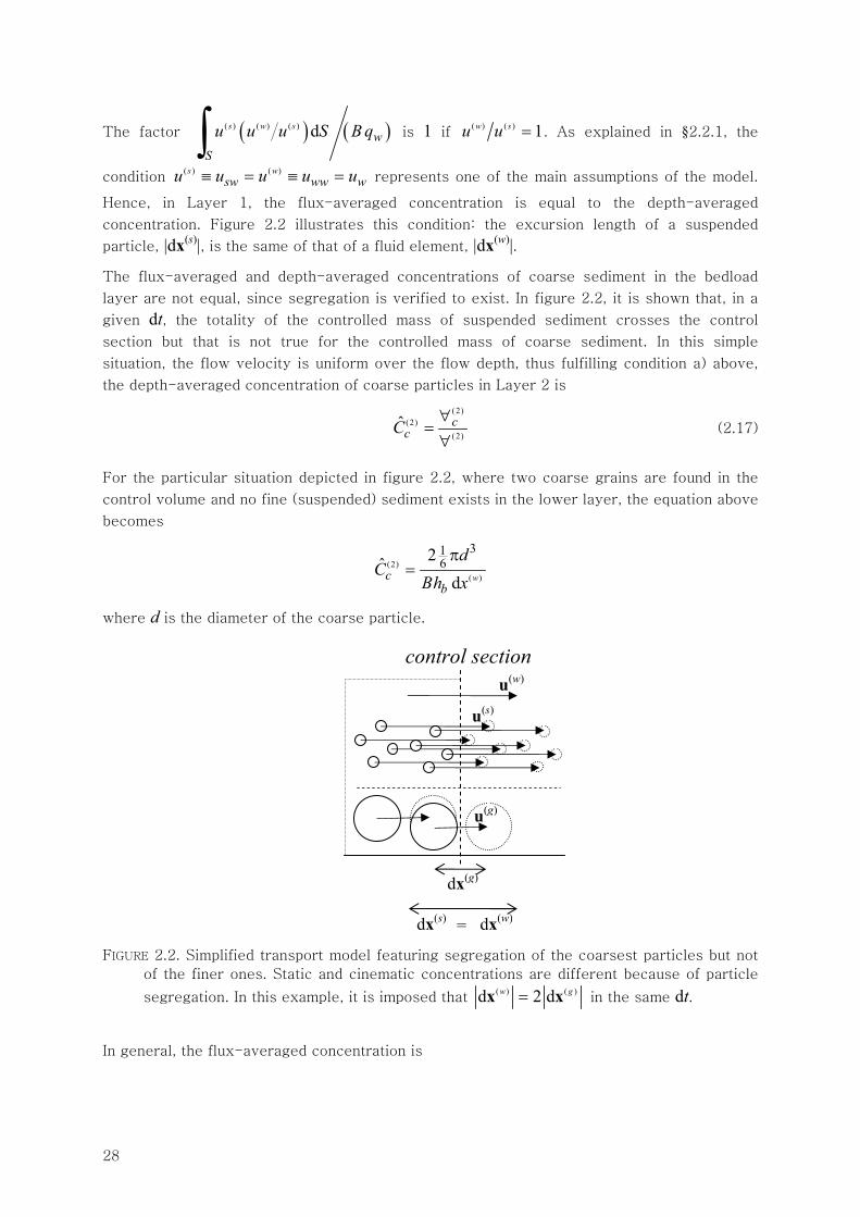
The flux-averaged and depth-averaged concentrations of coarse sediment in the bedload

layer are not equal, since segregation is verified to exist. In figure 2.2, it is shown that, in a

given dt, the totality of the controlled mass of suspended sediment crosses the control

section but that is not true for the controlled mass of coarse sediment. In this simple

situation, the flow velocity is uniform over the flow depth, thus fulfilling condition a) above,

the depth-averaged concentration of coarse particles in Layer 2 is

(2)(2)

(2)ˆ ccC

∀=∀

(2.17)

For the particular situation depicted in figure 2.2, where two coarse grains are found in the

control volume and no fine (suspended) sediment exists in the lower layer, the equation above

becomes

(2)

( )

3162ˆ

d wcb

dC

Bh xπ

=

where d is the diameter of the coarse particle.

FIGURE 2.2. Simplified transport model featuring segregation of the coarsest particles but not

of the finer ones. Static and cinematic concentrations are different because of particle

segregation. In this example, it is imposed that ( ) ( )d 2 dw g=x x in the same dt.

In general, the flux-averaged concentration is

u(w)

u(s)

u(g)

dx(g)

dx(s) dx(w)

control section

=

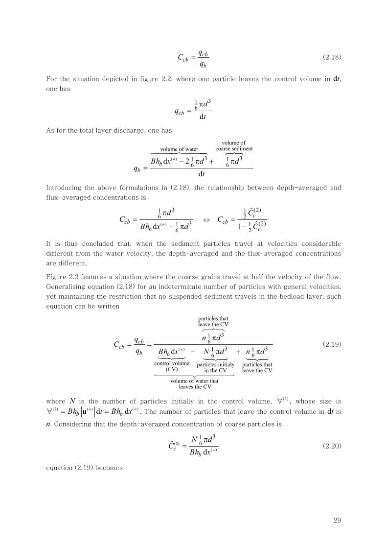
29

cbcb

b

qC

q= (2.18)

For the situation depicted in figure 2.2, where one particle leaves the control volume in dt, one has

316

dcbd

qt

π=

As for the total layer discharge, one has

( )

volume of coarse sedimentvolume of water

3 31 16 6d 2

d

wb

bBh x d d

qt

− π + π=

Introducing the above formulations in (2.18), the relationship between depth-averaged and

flux-averaged concentrations is

( )

316

316d wcb

b

dC

Bh x d

π=

− π ⇔

(2)12

(2)12

ˆ

ˆ1c

cbc

CC

C=

−

It is thus concluded that, when the sediment particles travel at velocities considerable

different from the water velocity, the depth-averaged and the flux-averaged concentrations

are different.

Figure 2.2 features a situation where the coarse grains travel at half the velocity of the flow.

Generalising equation (2.18) for an indeterminate number of particles with general velocities,

yet maintaining the restriction that no suspended sediment travels in the bedload layer, such

equation can be written

( )

particles thatleave the CV

316

3 31 16 6

control volume particles initialy particles that(CV) in the CV leave the CV

volume of water that leaves the CV

d w

cbcb

b b

n dqC

q Bh x N d n d

π= =

− π + π (2.19)

where N is the number of particles initially in the control volume, (2)∀ , whose size is

(2) ( ) ( )d dw wb bBh t Bh x∀ = =u . The number of particles that leave the control volume in dt is

n. Considering that the depth-averaged concentration of coarse particles is

(2)

( )

316ˆ

d wcb

N dC

Bh xπ

= (2.20)

equation (2.19) becomes

30

(2)( )

(2)

( ) ( )

316

3 31 16 6

ˆd

ˆ1 11d d

w

w w

cb

cb

cb b

N dn n CN Bh x NCnN d N dn CNBh x N Bh x

π

= =⎛ ⎞π π − −⎜ ⎟− + ⎝ ⎠

(2.21)

The fluid velocity in the bedload layer may be expressed as *wb wu u= α , where

( )*

wbu = τ ρ is the friction velocity. As for the mean velocity of the coarse grains, data

from Fernandez-Luque & van Beek (1976) may be used to show that *cb cu u= α where

c wα < α . Thus, the relation between wbu and cbu can be written

*wb cbu u= α (2.22)

where * 1α > . If the particles are homogeneously distributed in the layer, then *N n= α . In

general, the particles are not evenly distributed in the control volume. For instance, some

degree of spatial coherence is expected if bedload sheets are present. Nevertheless, if qcb in

(2.19) is understood as a mean value of a sufficiently long temporal series or an ensemble

average of a large number of realizations, it is likely that

*

1n nN N

≈ =α

(2.23)

In this case, equation (2.21) becomes

( )(2)

*

(2)

*

1

1

ˆ

ˆ1 1

ccb

c

CC

C

α

α

=− −

(2.24)

and, reciprocally,

( )

(2) *

*

ˆ1 1

cbc

cb

CC

Cα

=+ α −

(2.25)

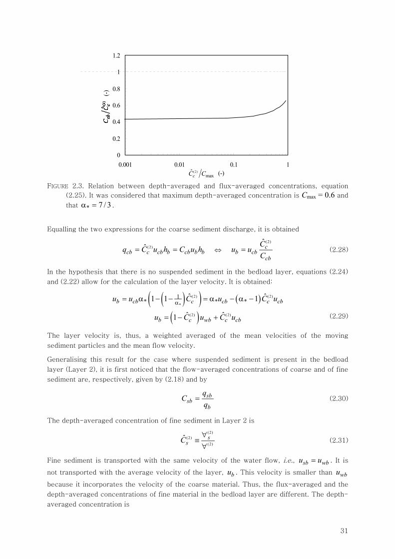
Equation (2.24) is graphically depicted in figure 2.3 for * 7 / 3α = and, hence, *

1 0.429α ≈ . It

is clear that, for (2)

maxˆ 0.3cC C < it is

(2)

*

1 ˆcb cC Cα≈ . Since it is expected that the bedload

concentrations do not exceed 0.1 (see §2.4.6, p. 133), it is legitimate to consider that the

relation between depth- and flux-averaged concentrations is

(2)

*

1 ˆcb cC Cα= and

(2)*

ˆc cbC C= α (2.26)(a) and (b)

The sediment discharge of coarse material is, from (2.18), determined by

cb cb b bq C u h= (2.27)

where ub is the mean layer velocity, understood as a continuum. The total discharge must be

the same whether expressed in terms of the depth-averaged or of flux-averaged

concentrations.

31

0

0.2

0.4

0.6

0.8

1

1.2

0.001 0.01 0.1 1C (2)/C max (-)

Ccb

/C(2

) (-)

FIGURE 2.3. Relation between depth-averaged and flux-averaged concentrations, equation

(2.25). It was considered that maximum depth-averaged concentration is Cmax = 0.6 and

that * 7 / 3α = .

Equalling the two expressions for the coarse sediment discharge, it is obtained

(2)ˆ

cb c cb b cb b bq C u h C u h= = ⇔

(2)ˆc

b cbcb

Cu u

C= (2.28)

In the hypothesis that there is no suspended sediment in the bedload layer, equations (2.24)

and (2.22) allow for the calculation of the layer velocity. It is obtained:

( )( ) ( )

( )

(2) (2)

*

(2) (2)

1* * *

ˆ ˆ1 1 1

ˆ ˆ1

b cb c cb c cb

b c wb c cb

u u C u C u

u C u C u

α= α − − = α − α −

= − +

(2.29)

The layer velocity is, thus, a weighted averaged of the mean velocities of the moving

sediment particles and the mean flow velocity.

Generalising this result for the case where suspended sediment is present in the bedload

layer (Layer 2), it is first noticed that the flow-averaged concentrations of coarse and of fine

sediment are, respectively, given by (2.18) and by

sbsb

b

qC

q= (2.30)

The depth-averaged concentration of fine sediment in Layer 2 is

(2)(2)

(2)ˆ s

sC∀

≡∀

(2.31)

Fine sediment is transported with the same velocity of the water flow, i.e., sb wbu u= . It is

not transported with the average velocity of the layer, bu . This velocity is smaller than wbu

because it incorporates the velocity of the coarse material. Thus, the flux-averaged and the

depth-averaged concentrations of fine material in the bedload layer are different. The depth-

averaged concentration is

(2)max

ˆcC C

32

(2)ˆ bs sb

wb

uC C

u= (2.32)

and, since wb bu u> , one has (2)ˆs sbC C< . The total sediment discharge in Layer 2, called

near-bed sediment discharge, qnb, is a simple summation of coarse and fine material

nb sb cbq q q= + ⇔ nb sb b b cb b bq C h u C h u= + (2.33)

If it written in terms of depth-averaged concentrations, one has

(2) (2) (2) (2)ˆ ˆ ˆ ˆ

nb c cb b s sb b c cb b s wb bq C u h C u h C u h C u h= + = + (2.34)

It is also convenient to express the total sediment discharge in Layer 2 in terms of a flux-

averaged concentration Cb, i.e., nb b b bq C h u= . From (2.33) it is obvious that

nbb sb cb

b

qC C C

q= = + (2.35)

Since the water discharge in Layer 2 is ( )1wb b nb b bq q q C q= − = − , one has

( )( )1wb cb sb b bq C C u h= − + (2.36)

Obviously, the water discharge can also be expressed in terms of water velocities and depth-

averaged concentrations. In that case, since a simple volume analysis reveals that

( )(2) (2)ˆ ˆ1wb c s wb bq C C u h= − − (2.37)

The total layer discharge is

b nb wb b bq q q u h= + = (2.38)

Introducing (2.37) and (2.34) in (2.38) one obtains

( )(2) (2) (2) (2)ˆ ˆ ˆ ˆ1b cb c wb s wb c su u C u C u C C= + + − − (2.39)

Equation (2.39) generalises equation (2.29): the layer velocity is the weighted average of the

velocities of each sediment class and of the water velocity. The weighting coefficients of

each sediment class are corresponding depth-averaged concentrations. Note that, (2.39)

bears the hypothesis sb wbu u= . This definition maintains the Eulerian nature of the

description: on a given instant and on a given location the mean velocity is an average of the

velocities of the different constituents at that location and at that time.

Flux-averaged concentrations are easier to determine than depth-averaged ones. Thus, it is

convenient to express bu as a function of cbC and of sbC . From equations (2.39) and (2.32)

one can express the depth-average suspended sediment concentration as

(2) (2) (2)ˆ ˆ ˆ1cbs sb c c

wb

uC C C C

u⎛ ⎞

= + −⎜ ⎟⎝ ⎠

Introducing (2.22) and (2.26), one obtains

( )( )(2)* *

ˆ 1 1s sb cb sbC C C C= − α − = β (2.40)

33

where ( )* *1 1cbCβ = − α − . As for the layer velocity, it is

( )( )*1 1b wb cbu u C= − α − (2.41)

These equations fully determine the depth-averaged concentration of fine sediment and the

layer velocity. Note that the flux-averaged concentrations and the velocity of the water are

easy to measure. They are valid for max *0.3cbC C< α , which, for max 0.6C = and

* 7 / 3α = , is 0.1cbC < , approximately. If that is not the case, full equation (2.24) should be

used instead of (2.26).

Having stated the averaged concentrations in Layers 1 and 2 and the corresponding layer

velocities and discharges, it is now necessary to determine the relation between the mac-

roscopic flow variables, h, u, and C, being C the total flow-averaged sediment concentration,

u the depth-averaged velocity and h the flow depth.

The total flow velocity is obtained by a layer-averaging process. Hence

( )1b wu q q

h= + ⇔ b w b b w w

b w b w

q q h u h uu

h h h h+ +

= =+ +

(2.42)

where qw is the discharge in Layer 1.

The total sediment discharge is

s sw cb sb nb swq q q q q q= + + = + ⇔ s b b b s w wq C h u C h u= + (2.43)

The total flux-averaged concentration can be defined from the total discharge. One has

sq Chu= ⇔ sqC

q=

sb b b cb b b s w wC h u C h u C h uC

hu+ +

= ⇔ b b b s w wC h u C h uC

hu+

= (2.44)

Equation (2.44) shows that the flux-averaged concentration can be seen as a layer-averaged

concentration. The concentration of each layer is weighted by the correspondent total layer

discharge.

In Layer 1, the depth-averaged apparent density of the suspended sediment is

(1) (1) ( ) (1) ( ) (1)

0 0

1 1 ˆˆ ( ) d ( )dw w

g g

h h

s s s sw w

C Ch h

ρ = ρ ξ ξ = ρ ξ ξ = ρ∫ ∫ (2.45)

Performing a similar integration, the apparent density of the water is ( )(1) ( ) (1)ˆˆ 1gw sCρ = ρ − .

Performing similar integrations, the depth-averaged apparent densities in Layer 2 are (2) ( ) (2)ˆˆ gs sCρ = ρ ,

(2) ( ) (2)ˆˆ gc cCρ = ρ and ( )(2) ( ) (2) (2)ˆ ˆˆ 1g

w s cC Cρ = ρ − − , respectively for the fine

sediment, coarse sediment and water.

The continuum layer densities will now be determined. For the suspended sediment layer

there is no segregation between water and sediment. Hence,

34

( ){ } ( )(1) ( ) (1) ( ) (1) ( ) (1) ( ) (1)ˆ ˆˆ 1 d 1w g w g

b

h

s s s sh

C C C Cρ = ρ − + ρ ξ = ρ − + ρ∫

( )(1) ( )ˆ 1 ( 1)ws ss Cρ = ρ = ρ + − (2.46)

For Layer 2, one has

( ){ }(2) ( ) (2) (2) ( ) (2) ( ) (2)

0

ˆ 1 db

w g g

h

s c s cC C C Cρ = ρ − − + ρ + ρ ξ∫

( )(2) ( ) (2) (2) ( ) (2) ( ) (2)ˆ ˆ ˆ ˆˆ 1w g gs c s cC C C Cρ = ρ − − + ρ + ρ

( )(2) ( ) (2) ( ) (2)ˆ ˆˆ 1w gC Cρ = ρ − + ρ ⇔ ( )(2) ( ) (2)ˆˆ 1 ( 1)w s Cρ = ρ + − (2.47)

The mixing layer and the substratum have the same apparent density. It is

( )( ) 1 ( 1)(1 )gbed s pρ = ρ + − − (2.48)

Flux-averaged concentrations allow for the determination of the following apparent densities.

For the suspended sediment layer one has ( )g

sw sCρ = ρ and ( )( ) 1www sCρ = ρ − for

suspended sediment and for water, respectively. Coarse and fine sediment in Layer 2 have,

respectively, ( )g

cb cbCρ = ρ and ( )g

sb sbCρ = ρ . The apparent density of water is

( )( ) 1wwb sb cbC Cρ = ρ − − .

The continuum layer density of the suspended sediment layer is

( )( ) ( ) 1g ws w w sw w w ww w w s w w s w wu h u h u h C u h C u hρ = ρ + ρ = ρ + ρ −

( ) ( )( ) ( ) ( )1 1 ( 1)g w gs s s sC C s Cρ = ρ + ρ − = ρ + − (2.49)

For the bedload layer, one has

b b b sb b b cb b b wb b bu h u h u h u hρ = ρ + ρ + ρ ⇔

⇔ ( ) ( )( ) ( ) 1g wb b b sb cb b b sb cb b bu h C C u h C C u hρ = ρ + + ρ − − ⇔

⇔ ( )( ) 1 ( 1)gb bs Cρ = ρ + − (2.50)

The apparent density of Layers 1 and 2 can be obtained from

( ) ( )( ) ( ) ( ) ( )1 1g g w wm b b b s w w b b b s w wuh C h u C h u Cuh C h u C h uρ = ρ + ρ + ρ − + ρ −

( )( ) ( ) 1g wmuh Cuh C uhρ = ρ + ρ − ⇔ ( )( ) 1 ( 1)g

b s Cρ = ρ + − (2.51)

The most relevant depth- and flow-averaged quantities in each layer are now determined.

The continuum conservation equations can now be derived.

2.2.2.3 Equations of conservation of fluid and sediment mass

Conservation of fine sediment mass in Layers 1 is expressed by

( )(1) ( )d d dsist

sistt s t sM

∀

= ρ ∀∫

Reynolds’ transport theorem (cf. Currie 1980, p. 9) is used to obtain an Eulerian formulation

35

(1) (1) ( )

(1) (1)

d d d 0st s s r S

∀ ∂∀

ρ ∀ + ρ =∫ ∫ u ni (2.52)

The velocity ur is relative to the boundaries of the control volume. Expressing d∀ as d dx S

and performing a time integration one obtains

2 2 2

(1) (1) ( ) (1) ( )

(1) (1) (1)1 1 1 1 2( , ) ( , ) ( , )

d d d d d d ds s

t x t

t s s st x S x t t S x t S x t

S x t u S u S t⎧ ⎫⎪ ⎪ρ + − ρ + ρ⎨ ⎬⎪ ⎪⎩ ⎭∫ ∫ ∫ ∫ ∫ ∫

( ) ( ){ }2 2

(2) (1)

1 1

2,1 2,1 1,2 1,2ˆ ˆ d d 0t x

s st x

l l x t+ − ρ φ + ρ φ =∫ ∫ (2.53)

where 2,1φ and 1,2φ are, respectively, the downwards and upwards velocities associated the

vertical3 fluxes of sediment in and out of the control volume and is l2,1 and l1,2 are the

effective channel widths at the interface between Layers 1 and 2. They need not be equal

because some lateral areas might not contribute to the vertical exchange of sediment. It

should be noticed that the last term in (2.53) is the integral of the net sediment flux between

Layers 1 and 2.

Assuming, for the sake of simplicity, that the channel is prismatic, the accumulation term in

(2.53) is

(1) (1) (1) (1) (1) (1) (1)

(1) ( , )

ˆd db

h

s s s w s wS x t h

S l l h l hρ = ρ ξ = ρ = ρ∫ ∫ (2.54)

Under the same hypotheses, the convective terms in (2.53) are

(1) ( ) (1) (1) ( ) (1) (1) ( )

(1) ( , )

d ds s s

b

h

s s s wS x t h

u S l u l u hρ = ρ ξ = ρ∫ ∫

and, by definition (see equation (2.14)), one has

(1) (1) (1) (1)

s w sw w wl u h l u hρ ≡ ρ (2.55)

Introducing these equations in (2.53) and considering that (2) ( ) (2)ˆ gs sCρ = ρ and

(1) ( ) (1)ˆ gs sCρ = ρ ,

one has

( ) ( ){ }2 2 2

(1) (1) (1) (1)

1 21 1 1

ˆd d d dt x t

t w s sw w w sw w wx xt x t

l h x t l h u l h u tρ + − ρ + ρ∫ ∫ ∫

( ) ( ){ }2 2

( ) (2) ( ) (1)

1 1

2,1 2,1 1,2 1,2ˆ ˆ d d 0g g

t x

s st x

l C l C x t+ − ρ φ + ρ φ =∫ ∫

3 It is admitted that channel slopes are small; hence, the direction normal to the flow towards the free

surface is designated by vertical direction.

36

Applying Leibnitz rule to the time derivative of the integrals (cf. Abramowitz & Stegun 1964,

p. 11) one obtains

( ) ( )2 2 2 2

(1) (1) (1)

1 1 1 1

ˆ d d d dt x t x

t w s x sw w wt x t x

l h x t l h u x t∂ ρ + ∂ ρ∫ ∫ ∫ ∫

( ) ( ){ }2 2

( ) (2) ( ) (1)

1 1

2,1 2,1 1,2 1,2ˆ ˆ d d 0g g

t x

s st x

l C l C x t+ − ρ φ + ρ φ =∫ ∫ (2.56)

If the vertical sediment fluxes are ( ) ( )

, , 1, 2i is s i jC iφ = φ = , the net vertical fluxes become

{ }2

(2) (1)

1

2,1 2,1 1,22 1

1 dx

nets s s

x

xx x

φ = − −φ + φ− ∫

where x1 and x2 delimit a representative length along the channel where the net flux is

calculated. It should be noticed that

{ } ( )2 2

(2) (1)

1 1

2,1 1,2 2 1 2,1 2,1d dx x

net nets s s s

x x

x x x x−φ + φ = − − φ = − φ∫ ∫ (2.57)

Introducing (2.57) in (2.56), one has

( ) ( )2 2 2 2

(1)

1 1 1 1

ˆ d d d dt x t x

t w s x sw w wt x t x

h x t h u x t∂ ρ + ∂ ρ∫ ∫ ∫ ∫2 2

( )

1 1

2,1d d 0g

t xnets

t x

x t+ −ρ φ =∫ ∫

Because the control volume is of arbitrary shape, the integrand must be zero. Thus

( ) ( )(1)ˆt w s x sw w wh h u∂ ρ + ∂ ρ ( )2,1 0g net

s−ρ φ =

Considering that (1) ( ) (1)ˆˆ gs sCρ = ρ and that

(1)ˆs swC C= and dividing by ρ(g), one obtains

( ) ( )t s w x s w wC h C h u∂ + ∂ 2,1 0nets−φ = (2.58)

Equation (2.58) is the partial differential equation that expresses the conservation of fine

sediment in the suspended sediment layer.

It is unnecessary to repeat all the steps for the remaining layers and for the remaining flow

constituents. Thus, employing a symmetric reasoning, the equation of conservation of fine

sediment in Layer 2 is

( )(2)dt sM = (2) (2) ( )

(2) (2)

d d d 0st s s r S

∀ ∂∀

ρ ∀ + ρ =∫ ∫ u ni

( ) ( )(2)ˆt s b x sb b bC h C h u∂ + ∂ 3,2 2,1 0net net

s s−φ + φ = (2.59)

Obviously, there are two net fluxes of fine sediment in this layer; 2,1netsφ directed to the

suspended sediment layer and 3,2nets−φ , directed to the mixing layer.

37

The mass conservation of coarse sediment mass in layer 2 obeys to

( )(2)dt cM = (2) (2) ( )

(2) (2)

d d d 0ct c c r S

∀ ∂∀

ρ ∀ + ρ =∫ ∫ u ni

Following the same line of reasoning one has

( ) ( )(2)ˆt b c x cb b bh h u∂ ρ + ∂ ρ ( )3,2 0g net

c−ρ φ = (2.60)

The only net flux of coarse sediment occurs due to interactions with the bed. As stated

before, the suspended sediment layer does not carry sediment whose velocity is different

from that of the surrounding water flow. In (2.60), (2) ( ) (2)ˆˆ gc cbCρ = ρ and

( )gcb cbCρ = ρ but

(2)ˆcbcbC C≠ . Thus, if the differential equation is supposed to be expressed in terms of cbC , as

it is easier to compute, equation (2.26) must be invoked. Thus, one has

( ) ( )(2)ˆt b c x cb b bh C C u h∂ + ∂ 02,3 =φ− net

c ⇔

⇔ ( ) ( )*t b cb x cb b bh C C u h∂ α + ∂ 02,3 =φ− netc (2.61)

Equation (2.61) is the continuum conservation equation of coarse sediment in the bedload

layer.

The sediment mass conservation in the mixing layer is

( )(3)dt sM = (3)

(3)

d d 0t s∀

ρ ∀ =∫

and, since there is no movement in the bed,

( ) (1 )t aL p∂ − 3,2netc+φ 3,2

nets+φ 4,3

netc−φ 4,3 0net

s−φ = (2.62)

Likewise, in the substratum, one has

( ) (1 )t b aY L p∂ − − 4,3netc+φ 4,3 0net

s+φ = (2.63)

The conservation equations for the mass of water will now be determined. The conservation

of water in Layer 1 is

( )(1)dt wM = (1) (1) ( )

(1) (1)

d d d 0wt w w r S

∀ ∂∀

ρ ∀ + ρ =∫ ∫ u ni

The vertical fluxes are ( )(1) (1)1,2

ˆ1w sCφ = − φ and the apparent density is ( )(1) ( ) (1)ˆˆ 1ww sCρ = ρ − .

The continuum conservation equation is

( ) ( )(1) (1)ˆ ˆt w w x w w wh h u∂ ρ + ∂ ρ ( )2,1 0w net

w−ρ φ =

( )( ) ( )( )1 1t w sw x sw w wh C C h u∂ − + ∂ − 2,1 0netw−φ = (2.64)

The conservation of water in Layer 2 is

38

( )(2)dt wM = (2) (2) ( )

(1) (1)

d d d 0wt w w r S

∀ ∂∀

ρ ∀ + ρ =∫ ∫ u ni

Given that the vertical fluxes are ( )(2) (2) (2)2,1w s c jC Cφ = − − φ , j = 1 or 3, the continuum

conservation equation is

( ) ( )(2)ˆt b w x wb b bh h u∂ ρ + ∂ ρ ( ) ( )3,2 2,1 0w wnet net

w w−ρ φ + ρ φ =

The apparent densities are ( )(2) ( ) (2) (2)ˆ ˆˆ 1ww s cC Cρ = ρ − − and ( )( ) 1w

wb sb cbC Cρ = ρ − − . Hence

( )( ) ( )( )(2) (2)ˆ ˆ1 1t b s c x b b sb cbh C C h u C C∂ − − + ∂ − − 3,2 2,1 0net netw w−φ + φ = (2.65)

is the conservation equation for the mass of water in the bedload layer.

The conservation of the mass of water in the mixing layer and in the substratum is trivially

obtained if the reciprocal of the porosity, (1−p) is, in (2.62) and (2.63), substituted by the

porosity, p and if the vertical sediment fluxes are substituted by the corresponding water

fluxes. Thus, one has

( )t aL p∂ 3,2netw+φ 4,3 0net

w−φ = and ( )t b aY L p∂ − 4,3 0netw+φ = (2.66)(a) and (b)

It is not practical to work with water conservation equations. The non-linearity of the terms

in ( )(1 )iC− , which is bound to cause discretization problems, can easily be avoided if the

system of conservation laws features, along with sediment mass conservation, total mass

conservation equations instead of its fluid counterparts.

Total conservation equations for Layer 1 are obtained by summing (2.58) and (2.64). One has

( ) ( )( ) ( ) ( )( )1 1t sw w t w sw x sw w w x sw w wC h h C C h u C h u∂ + ∂ − + ∂ + ∂ − 2,1nets−φ 2,1 0net

w−φ =

( ) ( )t w x w wh h u∂ + ∂ 2,1 0net−φ = (2.67)

where 2,1netsφ + 2,1

netwφ 2,1

net= φ . Likewise, the total conservation equation for the bedload

layer is obtained from (2.59), (2.61) and (2.65). The equation reads

( ) ( ) ( )( )( ) ( ) ( )( )* * * *1

1t sb b t b cb t b sb cb

x sb b b x cb b b x b b sb cb

C h h C h C C

C h u C u h h u C C

∂ β + ∂ α + ∂ −β − α

+∂ + ∂ + ∂ − −

3,2 3,2 3,2 2,1 2,1 0net net net net nets c w s w−φ − φ − φ + φ + φ =

( ) ( )t b x b bh h u∂ + ∂ 3,2 2,1 0net net−φ + φ = (2.68)

where 3,2 3,2 3,2 3,2net net net nets c wφ + φ + φ = φ and 2,1 2,1 2,1

net net nets wφ + φ = φ because there is no

vertical flux of coarse sediment between layers 1 and 2.

As for the total mass conservation in the bed, one has, from (2.66)a) and b), (2.63) and (2.62)

( ) 3,2 0nett bY∂ + φ = (2.69)

39

The mass conservation equations drawn in this section can be further recombined to fit

numerical modelling requirements.

2.2.2.4 Equations of conservation of fluid and sediment momentum

The continuum approach followed in the previous section featured independent derivation of

the sediment and water mass conservation equations, followed by its summation. In this

section, the conservation of momentum will be derived for the sediment-water mixture,

considered as a homogeneous continuum. Later, the sediment contribution will be evaluated

so that simplifications can be discussed.

The conservation of momentum of a layer where the longitudinal velocity is not zero, for

instance Layer 2, is

( ) (2)(2)d d d dsist sist sist

t t b M SP S∀ ∀ ∂∀

= ρ ∀ = ∀ +∫ ∫ ∫u f f d (2.70)

where (2)P is the momentum in Layer 2, fM represents the mass forces and fS the surface

forces. If the equation of conservation of momentum is derived within the continuum

hypothesis, flux-averaged quantities must be used. The layer density is, it should be

remembered, ( )( ) 1 ( 1)wb bs Cρ = ρ + − . The external forces in the above equation can be

divided into pressure and stress forces. The equation becomes

(2) (2) (2)

(2) (2) (2) (2) (2)

d d d d d dt b b r bu S S S∀ ∂∀ ∀ ∂∀ ∂∀

ρ ∀ + ρ = ρ ∀+ +∫ ∫ ∫ ∫ ∫u u n g σ τi

where g stands for the acceleration of gravity, σ stands the pressure forces and τ stands for

the tangential forces.

In the along stream direction, the left-hand member is, after a time integration in a one-

dimensional channel

2 2(2)

(1)1 1 ( , )

d d d dt x

t bt x S x t

LHx u S x t= ρ∫ ∫ ∫

( ) ( )2

(2) (2)

(2) (2)1 1 2

2 2

( , ) ( , )

d d dt

b bt S x t S x t

u S u S t⎧ ⎫⎪ ⎪+ − ρ + ρ⎨ ⎬⎪ ⎪⎩ ⎭∫ ∫ ∫

( ) ( ){ }2 2

1 1

2,1 2,1 1,2 1,2 d dt x

s w b bt x

l u l u x t+ − ρ φ + ρ φ∫ ∫ (2.71)

The vertical fluxes of momentum are originated by the fact that when a parcel of fluid or of

sediment changes layer it does so bringing with it the longitudinal velocity of the original

layer. The net momentum flux is

( ) ( ){ }2 2

( ) (2)

1 1

2,1 2,1 1,2 1,2 2,1d dw

x xnet

s w b b Ix x

l u l u x l u x− ρ φ + ρ φ = − ρ φ∫ ∫ (2.72)

40

where Iu is a representative longitudinal velocity, defined as a combination of the velocities

and densities of the adjacent layers.

Introducing (2.72) in (2.71) and performing the integration of the velocities over the layer

cross-section, one obtains

2 2(2)

1 1

d d dt x

t b b bt x

LHx l h u x t= ρ∫ ∫ ( )( ) ( )( )2

(2) (2)

1 21

2 2 dt

b b b b b bx xt

l h u l h u t⎧ ⎫

+ − ρ + ρ⎨ ⎬⎩ ⎭∫

2 2( ) (2)

1 1

2,1 dw

t xnet

It x

l u x− ρ φ∫ ∫

Applying the Leibnitz rule, one has

( ) ( )( )2 2 2 2

(2) (2)

1 1 1 1

2d d d dt x t x

t b b b x b b b bt x t x

LHx l h u x t l h u u x t= ∂ ρ + ∂ ρ∫ ∫ ∫ ∫

2 2( ) (2)

1 1

2,1 dw

t xnet

It x

l u x− ρ φ∫ ∫ (2.73)

Because the channel is wide and prismatic,

( ) ( )( )2 2 2 2

1 1 1 1

2d d d dt x t x

t b b b x b b bt x t x

LHx B h u x t h u x t= ∂ ρ + ∂ ρ∫ ∫ ∫ ∫

2 2( )

1 1

2,1 dw

t xnet

It x

u x− ρ φ∫ ∫ (2.74)

As for the right-hand member, assuming that the channel is wide and prismatic, it becomes

2 2(2)

1 1

d dt x

x b bt x

RHx g l h x t= ρ∫ ∫

( )( ) ( )( )2

(2) (2) (2) (2)

1 21

2 21 12 2 d

t

b b s w b b b s w bx xt

g l h l h h l h l h h t⎧ ⎫

+ ρ + ρ − ρ + ρ⎨ ⎬⎩ ⎭∫

2 2 2 2

1 1 1 1

3,2 3,2 2,1 2,1d d d dt x t x

t x t x

l x t l x t+ τ − τ∫ ∫ ∫ ∫ ⇔

⇔ ( )( )1 2 1 2

1 1 1 1

212d d d d

t x t x

x b b x b b s w bt x t x

RHx B g h x t g h h h x t= ρ + ∂ ρ + ρ∫ ∫ ∫ ∫

2 2 2 2

1 1 1 1

3,2 2,1d d d dt x t x

t x t x

x t x t+ τ − τ∫ ∫ ∫ ∫ (2.75)

41

The only mass force per unit mass is the force of gravity, whose component in the along-

stream direction is ( )( )sin( )x x bg g g Y= θ = −∂ .

Considering that the volume is arbitrary and equating (2.74) and (2.75), one obtains

( ) ( ) ( ) ( )2 212,12 2 w net

t b b b x b b b x s w b b b Iu h u h g h h h u∂ ρ + ∂ ρ + ∂ ρ + ρ = ρ φ

( )b b x bg h Y− ρ ∂ 1,22,3 τ−τ+ (2.76)

Equation (2.76) is the momentum conservation equation of the bedload layer, idealized as a

continuum. Using a symmetric algebraic process, the equation of momentum conservation of

the suspended sediment layer is

( ) ( ) ( ) ( )( )2 212,1 2,12

w nett s w w x s w w x s w I s w x bu h u h g h u g h Y∂ ρ + ∂ ρ + ∂ ρ = ρ φ − ρ ∂ + τ (2.77)

It is reasonable to discuss whether or not the momentum transported by the coarse particles

in the bedload layer is relevant in the total balance, given that the mass of water in the

overall flow is much greater than the mass of the coarse particles. If the momentum

associated to the coarse particles can be discarded, the overall momentum conservation can

be greatly simplified, which greatly favours the efficiency of the solution procedures.

2.2.2.5 Conservation of momentum of the coarse particles in the bedload layer

The momentum balance for the coarse particles transported in the bedload layer is expressed

by a conservation equation whose derivation does not follow the application of Reynolds’ transport theorem. This is so because the system is composed of a discrete particle set.

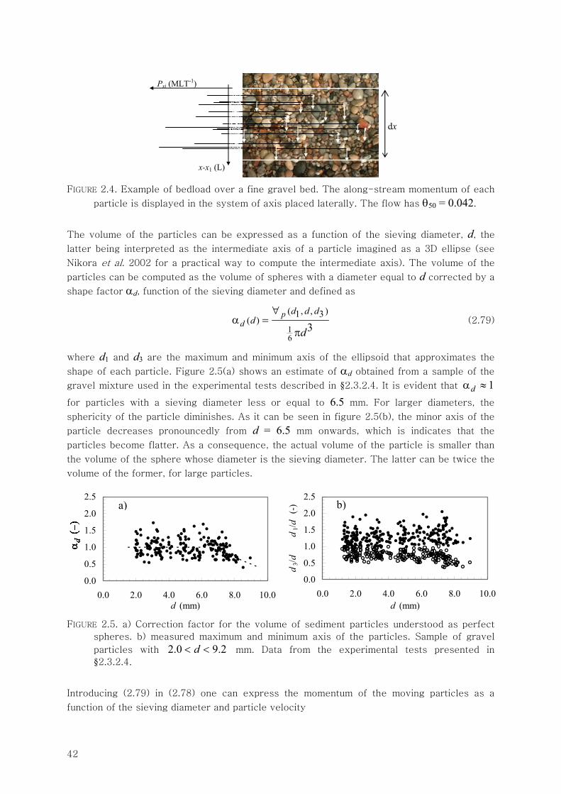
Figure 2.4 displays a typical flow situation, taken from a still image of the video footing of an

experimental gravel transport test (see §2.3.2.4, p. 67 and following). The bed is composed of

fine gravel and some of the grains are moving with a downstream velocity represented by the

white arrows.

In the along-stream direction, dPs is the momentum of the set of moving particles contained,

at a given instant, in a strip of length dx, arbitrarily small, and is computed as

( )

1

d g

n

s pi pi

i

P u

=

= ρ ∀∑ (2.78)

where upi and ∀pi are, respectively, the velocity and the volume of each of the mobile

particles, n is the number of moving particles in the strip and ρ(g) is the density of the

particles, assumed equal for all the bed particles. The momentum, in the along-stream

direction, of each particle in the strip of length dx can be seen in figure 2.4, in the frame

whose x-axis runs along stream.

This is an Eulerian, rather than Lagrangean, account of the momentum associated to the

moving particles, for it is taken at a given instant in an arbitrary domain and not from a fixed

set of chosen particles followed over the time. The Eulerian account is desirable to ensure

compatibility with the remaining conservation equations, since they were obtained, through

Reynolds’ transport theorem, on such grounds. It should be noticed that both Eulerian and

Lagrangean accounts would be equivalent only if the followed particles were the same ones

that would turn out at the sediment sampler as a bedload sample.

42

FIGURE 2.4. Example of bedload over a fine gravel bed. The along-stream momentum of each

particle is displayed in the system of axis placed laterally. The flow has θ50 = 0.042.

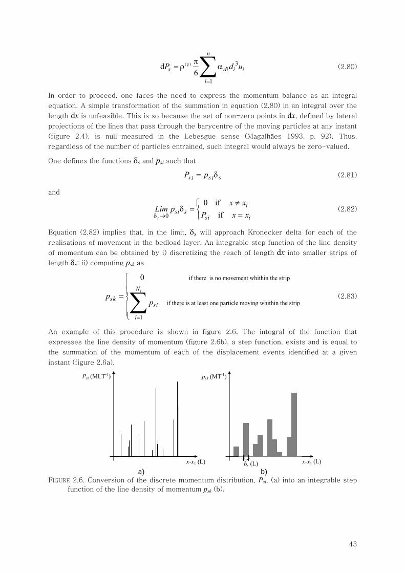
The volume of the particles can be expressed as a function of the sieving diameter, d, the

latter being interpreted as the intermediate axis of a particle imagined as a 3D ellipse (see

Nikora et al. 2002 for a practical way to compute the intermediate axis). The volume of the

particles can be computed as the volume of spheres with a diameter equal to d corrected by a

shape factor αd, function of the sieving diameter and defined as

16

( , , )1 3( )

3p

dd d d

dd

∀α =

π (2.79)

where d1 and d3 are the maximum and minimum axis of the ellipsoid that approximates the

shape of each particle. Figure 2.5(a) shows an estimate of αd obtained from a sample of the

gravel mixture used in the experimental tests described in §2.3.2.4. It is evident that 1dα ≈

for particles with a sieving diameter less or equal to 6.5 mm. For larger diameters, the

sphericity of the particle diminishes. As it can be seen in figure 2.5(b), the minor axis of the

particle decreases pronouncedly from d = 6.5 mm onwards, which is indicates that the

particles become flatter. As a consequence, the actual volume of the particle is smaller than

the volume of the sphere whose diameter is the sieving diameter. The latter can be twice the

volume of the former, for large particles.

0.0

0.5

1.0

1.5

2.0

2.5

0.0 2.0 4.0 6.0 8.0 10.0d (mm)

⊗ d (-

)

0.0

0.5

1.0

1.5

2.0

2.5

0.0 2.0 4.0 6.0 8.0 10.0d (mm)

d3/d

d1/d

(-

)

FIGURE 2.5. a) Correction factor for the volume of sediment particles understood as perfect

spheres. b) measured maximum and minimum axis of the particles. Sample of gravel

particles with 2.0 9.2d< < mm. Data from the experimental tests presented in

§2.3.2.4.

Introducing (2.79) in (2.78) one can express the momentum of the moving particles as a

function of the sieving diameter and particle velocity

dx

Psi (MLT-1)

x-x1 (L)

a) b)

43

( ) 3

1

d6

g

n

s di i i

i

P d u

=

π= ρ α∑ (2.80)

In order to proceed, one faces the need to express the momentum balance as an integral

equation. A simple transformation of the summation in equation (2.80) in an integral over the

length dx is unfeasible. This is so because the set of non-zero points in dx, defined by lateral

projections of the lines that pass through the barycentre of the moving particles at any instant

(figure 2.4), is null-measured in the Lebesgue sense (Magalhães 1993, p. 92). Thus,

regardless of the number of particles entrained, such integral would always be zero-valued.

One defines the functions δs and psi such that

sisis pP δ= (2.81)

and

0

0 ififs

isi s

si i

x xLim p

P x xδ →

≠⎧δ = ⎨ =⎩

(2.82)

Equation (2.82) implies that, in the limit, δs will approach Kronecker delta for each of the

realisations of movement in the bedload layer. An integrable step function of the line density

of momentum can be obtained by i) discretizing the reach of length dx into smaller strips of

length δs; ii) computing psk as

if there is no movement whithin the strip

if there is at least one particle moving whithin the strip

1

0 iN

sksi

i

pp

=

⎧⎪⎪= ⎨⎪⎪⎩∑ (2.83)

An example of this procedure is shown in figure 2.6. The integral of the function that

expresses the line density of momentum (figure 2.6b), a step function, exists and is equal to

the summation of the momentum of each of the displacement events identified at a given

instant (figure 2.6a).

a) b)

FIGURE 2.6. Conversion of the discrete momentum distribution, Psi, (a) into an integrable step

function of the line density of momentum psk (b).

Psi (MLT-1)

x-x1 (L)

psk (MT-1)

x-x1 (L) δs (L)

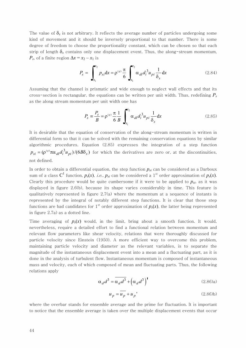
44

The value of δs is not arbitrary. It reflects the average number of particles undergoing some

kind of movement and it should be inversely proportional to that number. There is some

degree of freedom to choose the proportionality constant, which can be chosen so that each

strip of length δs contains only one displacement event. Thus, the along-stream momentum,

Ps, of a finite region Δx = x2 – x1 is

2 2( )

1 1

3 1d d6

g

x x

s si di i pisx x

P p x d u xπ= = ρ α

δ∫ ∫ (2.84)

Assuming that the channel is prismatic and wide enough to neglect wall effects and that its

cross-section is rectangular, the equations can be written per unit width. Thus, redefining Ps

as the along stream momentum per unit width one has

2( )

1

31 1 d6

g

xs

s di i pisx

PP d u x

B Bπ

≡ = ρ αδ∫ (2.85)

It is desirable that the equation of conservation of the along-stream momentum is written in

differential form so that it can be solved with the remaining conservation equations by similar

algorithmic procedures. Equation (2.85) expresses the integration of a step function ( ) 3( ) /(6 )g

si di i pi sp d u B= ρ πα δ for which the derivatives are zero or, at the discontinuities,

not defined.

In order to obtain a differential equation, the step function psi can be considered as a Darboux

sum of a class C1 function, ps(x), i.e., psi can be considered a 1st order approximation of ps(x).

Clearly this procedure would be quite cumbersome if it were to be applied to psi, as it was

displayed in figure 2.6(b), because its shape varies considerably in time. This feature is

qualitatively represented in figure 2.7(a) where the momentum at a sequence of instants is

represented by the integral of notably different step functions. It is clear that those step

functions are bad candidates for 1st order approximation of ps(x), the latter being represented

in figure 2.7a) as a dotted line.

Time averaging of ps(x) would, in the limit, bring about a smooth function. It would,

nevertheless, require a detailed effort to find a functional relation between momentum and

relevant flow parameters like shear velocity, relations that were thoroughly discussed for

particle velocity since Einstein (1950). A more efficient way to overcome this problem,

maintaining particle velocity and diameter as the relevant variables, is to separate the

magnitude of the instantaneous displacement event into a mean and a fluctuating part, as it is

done in the analysis of turbulent flow. Instantaneous momentum is composed of instantaneous

mass and velocity, each of which composed of mean and fluctuating parts. Thus, the following

relations apply

( )3 3 3 'd d dd d dα = α + α (2.86)a)

'ppp uuu += (2.86)b)

where the overbar stands for ensemble average and the prime for fluctuation. It is important

to notice that the ensemble average is taken over the multiple displacement events that occur

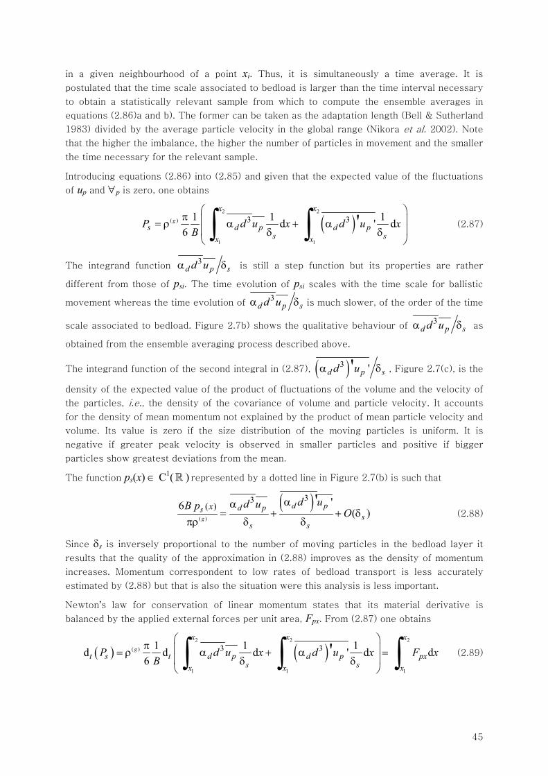
45

in a given neighbourhood of a point xi. Thus, it is simultaneously a time average. It is

postulated that the time scale associated to bedload is larger than the time interval necessary

to obtain a statistically relevant sample from which to compute the ensemble averages in

equations (2.86)a and b). The former can be taken as the adaptation length (Bell & Sutherland

1983) divided by the average particle velocity in the global range (Nikora et al. 2002). Note

that the higher the imbalance, the higher the number of particles in movement and the smaller

the time necessary for the relevant sample.

Introducing equations (2.86) into (2.85) and given that the expected value of the fluctuations

of up and ∀p is zero, one obtains

( )2 2

( )

1 1

3 31 1 1d ' d6

'g

x x

s d p d ps sx x

P d u x d u xB

⎛ ⎞π ⎜ ⎟= ρ α + α⎜ ⎟δ δ⎝ ⎠∫ ∫ (2.87)

The integrand function 3

d p sd uα δ is still a step function but its properties are rather

different from those of psi. The time evolution of psi scales with the time scale for ballistic

movement whereas the time evolution of 3

d p sd uα δ is much slower, of the order of the time

scale associated to bedload. Figure 2.7b) shows the qualitative behaviour of 3

d p sd uα δ as

obtained from the ensemble averaging process described above.

The integrand function of the second integral in (2.87), ( )3 ''d p sd uα δ , Figure 2.7(c), is the

density of the expected value of the product of fluctuations of the volume and the velocity of

the particles, i.e., the density of the covariance of volume and particle velocity. It accounts

for the density of mean momentum not explained by the product of mean particle velocity and

volume. Its value is zero if the size distribution of the moving particles is uniform. It is

negative if greater peak velocity is observed in smaller particles and positive if bigger

particles show greatest deviations from the mean.

The function ps(x) ∈ C1( ) represented by a dotted line in Figure 2.7(b) is such that

( )

( )

33( ) '6

( )'

g

d pd pss

s s

x d ud uB pO

αα= + + δ

πρ δ δ (2.88)

Since δs is inversely proportional to the number of moving particles in the bedload layer it

results that the quality of the approximation in (2.88) improves as the density of momentum

increases. Momentum correspondent to low rates of bedload transport is less accurately

estimated by (2.88) but that is also the situation were this analysis is less important.

Newton’s law for conservation of linear momentum states that its material derivative is

balanced by the applied external forces per unit area, Fpx. From (2.87) one obtains

( ) ( )2 2 2

( )

1 1 1

3 31 1 1d d d ' d d6

'g

x x x

t s t d p d p pxs sx x x

P d u x d u x F xB

⎛ ⎞π ⎜ ⎟= ρ α + α =⎜ ⎟δ δ⎝ ⎠∫ ∫ ∫ (2.89)

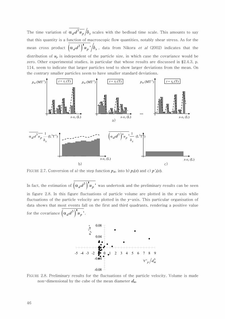
46

The time variation of 3

d p sd uα δ scales with the bedload time scale. This amounts to say

that this quantity is a function of macroscopic flow quantities, notably shear stress. As for the

mean cross product ( )3 ''d p sd uα δ , data from Nikora et al (2002) indicates that the

distribution of up is independent of the particle size, in which case the covariance would be

zero. Other experimental studies, in particular that whose results are discussed in §2.4.3, p.

114, seem to indicate that larger particles tend to show larger deviations from the mean. On

the contrary smaller particles seem to have smaller standard deviations.

FIGURE 2.7. Conversion of a) the step function psk, into b) ps(x) and c) p’s(x).

In fact, the estimation of ( )3 ''d pd uα was undertook and the preliminary results can be seen

in figure 2.8. In this figure fluctuations of particle volume are plotted in the x-axis while

fluctuations of the particle velocity are plotted in the y-axis. This particular organisation of

data shows that most events fall on the first and third quadrants, rendering a positive value

for the covariance ( )3 ''d pd uα .

-0.08

-0.04

0

0.04

0.08

-5 -4 -3 -2 -1 0 1 2 3 4 5 6 7 8 9

V p '/D m3

up

'/u*

FIGURE 2.8. Preliminary results for the fluctuations of the particle velocity. Volume is made

non-dimensional by the cube of the mean diameter dm.

psk (MT-1)

x-x1 (L)

t = t1 (T) psk (MT-1)

x-x1 (L)

t = t2 (T) psk (MT-1)

x-x1 (L)

t = tn (T)

( )3 1'' ps

ud dαδ

(L3T-1)

x-x1 (L)

3 1p

sd udα

δ(L3T-1)

x-x1 (L)

a)

b) c)

3'p md∀

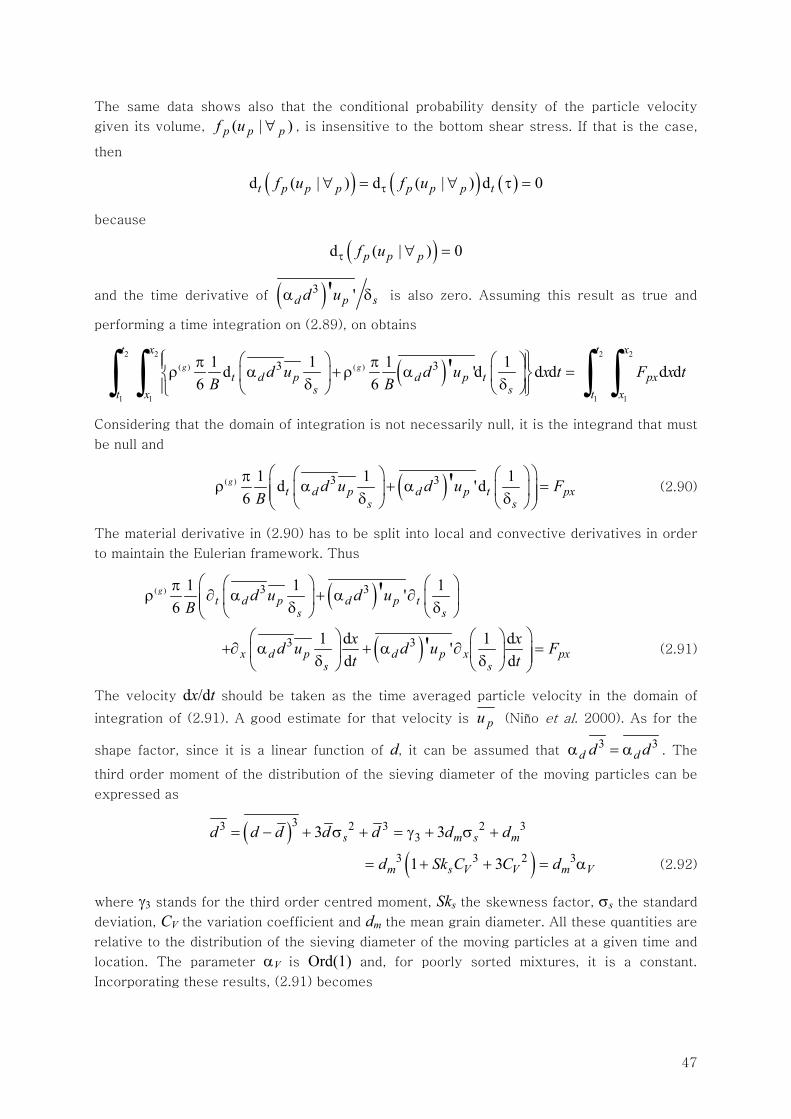
47

The same data shows also that the conditional probability density of the particle velocity

given its volume, )|( ppp uf ∀ , is insensitive to the bottom shear stress. If that is the case,

then

( ) ( ) ( )d ( | ) d ( | ) d 0t p p p p p p tf u f uτ∀ = ∀ τ =

because

( )d ( | ) 0p p pf uτ ∀ =

and the time derivative of ( )3 ''d p sd uα δ is also zero. Assuming this result as true and

performing a time integration on (2.89), on obtains

( )2 2 2 2

( ) ( )

1 1 1 1

3 31 1 1 1d 'd d d d d6 6

'g g

t x t x

t d p d p t pxs st x t x

d u d u x t F x tB B

⎧ ⎫⎛ ⎞ ⎛ ⎞π π⎪ ⎪ρ α + ρ α =⎨ ⎬⎜ ⎟ ⎜ ⎟δ δ⎪ ⎪⎝ ⎠ ⎝ ⎠⎩ ⎭∫ ∫ ∫ ∫

Considering that the domain of integration is not necessarily null, it is the integrand that must

be null and

( )( ) 3 31 1 1d 'd6

'gt d p d p t px

s sd u d u F

B⎛ ⎞⎛ ⎞ ⎛ ⎞π

ρ α + α =⎜ ⎟⎜ ⎟ ⎜ ⎟⎜ ⎟δ δ⎝ ⎠ ⎝ ⎠⎝ ⎠ (2.90)

The material derivative in (2.90) has to be split into local and convective derivatives in order

to maintain the Eulerian framework. Thus

( )( ) 3 31 1 1'6

'gt d p d p t

s sd u d u

B⎛ ⎛ ⎞ ⎛ ⎞π

ρ ∂ α + α ∂⎜ ⎜ ⎟ ⎜ ⎟⎜ δ δ⎝ ⎠ ⎝ ⎠⎝

( )3 31 d 1 d'd d

'x d p d p x pxs s

x xd u d u Ft t

⎞⎛ ⎞ ⎛ ⎞+∂ α + α ∂ =⎟⎜ ⎟ ⎜ ⎟ ⎟δ δ⎝ ⎠ ⎝ ⎠ ⎠

(2.91)

The velocity dx/dt should be taken as the time averaged particle velocity in the domain of

integration of (2.91). A good estimate for that velocity is pu (Niño et al. 2000). As for the

shape factor, since it is a linear function of d, it can be assumed that 3 3

d dd dα = α . The

third order moment of the distribution of the sieving diameter of the moving particles can be

expressed as

( )33 2 3 2 333 3s m s md d d d d d d= − + σ + = γ + σ +

( )3 3 2 31 3m s V V m Vd Sk C C d= + + = α (2.92)

where γ3 stands for the third order centred moment, Sks the skewness factor, σs the standard

deviation, CV the variation coefficient and dm the mean grain diameter. All these quantities are

relative to the distribution of the sieving diameter of the moving particles at a given time and

location. The parameter αV is Ord(1) and, for poorly sorted mixtures, it is a constant.

Incorporating these results, (2.91) becomes

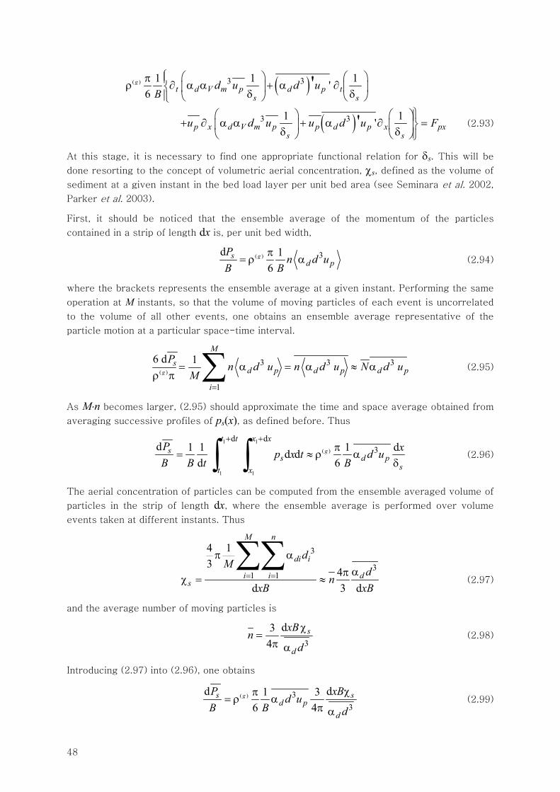
48

( )( ) 3 31 1 1'6

'gt d V m p d p t

s sd u d u

B⎧ ⎛ ⎞ ⎛ ⎞π ⎪ρ ∂ α α + α ∂⎨ ⎜ ⎟ ⎜ ⎟δ δ⎪ ⎝ ⎠ ⎝ ⎠⎩

( )3 31 1''p x d V m p p d p x pxs s

u d u u d u F⎫⎛ ⎞ ⎛ ⎞⎪+ ∂ α α + α ∂ =⎬⎜ ⎟ ⎜ ⎟δ δ ⎪⎝ ⎠ ⎝ ⎠⎭

(2.93)

At this stage, it is necessary to find one appropriate functional relation for δs. This will be

done resorting to the concept of volumetric aerial concentration, χs, defined as the volume of

sediment at a given instant in the bed load layer per unit bed area (see Seminara et al. 2002,

Parker et al. 2003).

First, it should be noticed that the ensemble average of the momentum of the particles

contained in a strip of length dx is, per unit bed width,

( ) 3d 1

6gs

d pP

n d uB B

π= ρ α (2.94)

where the brackets represents the ensemble average at a given instant. Performing the same

operation at M instants, so that the volume of moving particles of each event is uncorrelated

to the volume of all other events, one obtains an ensemble average representative of the

particle motion at a particular space-time interval.

( )

3 3 3

1

6 d 1g

M

sd p d p d p

i

Pn d u n d u N d u

M=

= α = α ≈ αρ π ∑ (2.95)

As M⋅n becomes larger, (2.95) should approximate the time and space average obtained from

averaging successive profiles of ps(x), as defined before. Thus

1 1( )

1 1

d d3d 1 1 1 dd d

d 6g

t t x xs

s d pst x

P xp x t d uB B t B

+ +π

= ≈ ρ αδ∫ ∫ (2.96)

The aerial concentration of particles can be computed from the ensemble averaged volume of

particles in the strip of length dx, where the ensemble average is performed over volume

events taken at different instants. Thus

3

31 1

4 13

4d 3 d

M n

di i

i i ds

dM

dn

xB xB= =

π ααπ

χ = ≈∑∑

(2.97)

and the average number of moving particles is

3

d34

s

d

xBn

d

χ=

π α (2.98)

Introducing (2.97) into (2.96), one obtains

( ) 3

3

d d1 36 4

gs sd p

d

P xBd u

B B d

χπ= ρ α

π α (2.99)

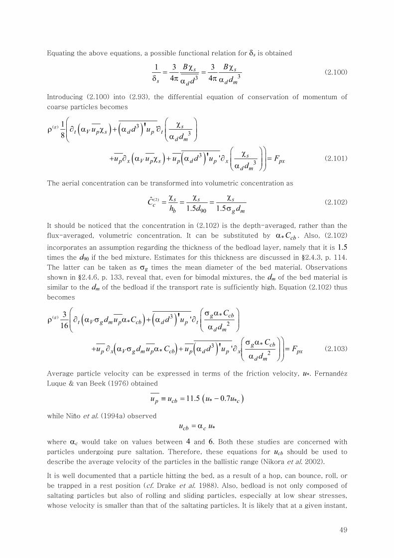
49

Equating the above equations, a possible functional relation for δs is obtained

33

1 3 34 4

s s

s d md

B Bdd

χ χ= =

δ π π αα (2.100)

Introducing (2.100) into (2.93), the differential equation of conservation of momentum of

coarse particles becomes

( ) ( )( ) 33

1 '8

'g st V p s d p t

d mu d u

d

⎛ ⎛ ⎞χ⎜ρ ∂ α χ + α ∂ ⎜ ⎟⎜ ⎟⎜ α⎝ ⎠⎝

( ) ( )33'' s

p x V p s p d p x pxd m

u u u d u Fd

⎞⎛ ⎞χ⎟+ ∂ α χ + α ∂ =⎜ ⎟⎜ ⎟⎟α⎝ ⎠⎠

(2.101)

The aerial concentration can be transformed into volumetric concentration as

(2)

90

ˆ1.5 1.5

s s sc

b g mC

h d dχ χ χ

= = =σ

(2.102)

It should be noticed that the concentration in (2.102) is the depth-averaged, rather than the

flux-averaged, volumetric concentration. It can be substituted by * cbCα . Also, (2.102)

incorporates an assumption regarding the thickness of the bedload layer, namely that it is 1.5

times the d90 if the bed mixture. Estimates for this thickness are discussed in §2.4.3, p. 114.

The latter can be taken as σg times the mean diameter of the bed material. Observations

shown in §2.4.6, p. 133, reveal that, even for bimodal mixtures, the dm of the bed material is

similar to the dm of the bedload if the transport rate is sufficiently high. Equation (2.102) thus

becomes

( ) ( )( ) *3* 2

3 '16

'g g cbt V g m p cb d p t

d m

Cd u C d u

d

⎛ ⎛ ⎞σ α⎜ρ ∂ α σ α + α ∂ ⎜ ⎟⎜ ⎟⎜ α⎝ ⎠⎝

( ) ( ) *3* 2'' g cb

p x V g m p cb p d p x pxd m

Cu d u C u d u F

d

⎞⎛ ⎞σ α⎟+ ∂ α σ α + α ∂ =⎜ ⎟⎜ ⎟⎟α⎝ ⎠⎠

(2.103)

Average particle velocity can be expressed in terms of the friction velocity, u*. Fernandéz

Luque & van Beek (1976) obtained

( )* *11.5 0.7p cb cu u u u≡ = −

while Niño et al. (1994a) observed

*cb cu u= α

where αc would take on values between 4 and 6. Both these studies are concerned with

particles undergoing pure saltation. Therefore, these equations for ucb should be used to

describe the average velocity of the particles in the ballistic range (Nikora et al. 2002).

It is well documented that a particle hitting the bed, as a result of a hop, can bounce, roll, or

be trapped in a rest position (cf. Drake et al. 1988). Also, bedload is not only composed of

saltating particles but also of rolling and sliding particles, especially at low shear stresses,

whose velocity is smaller than that of the saltating particles. It is likely that at a given instant,

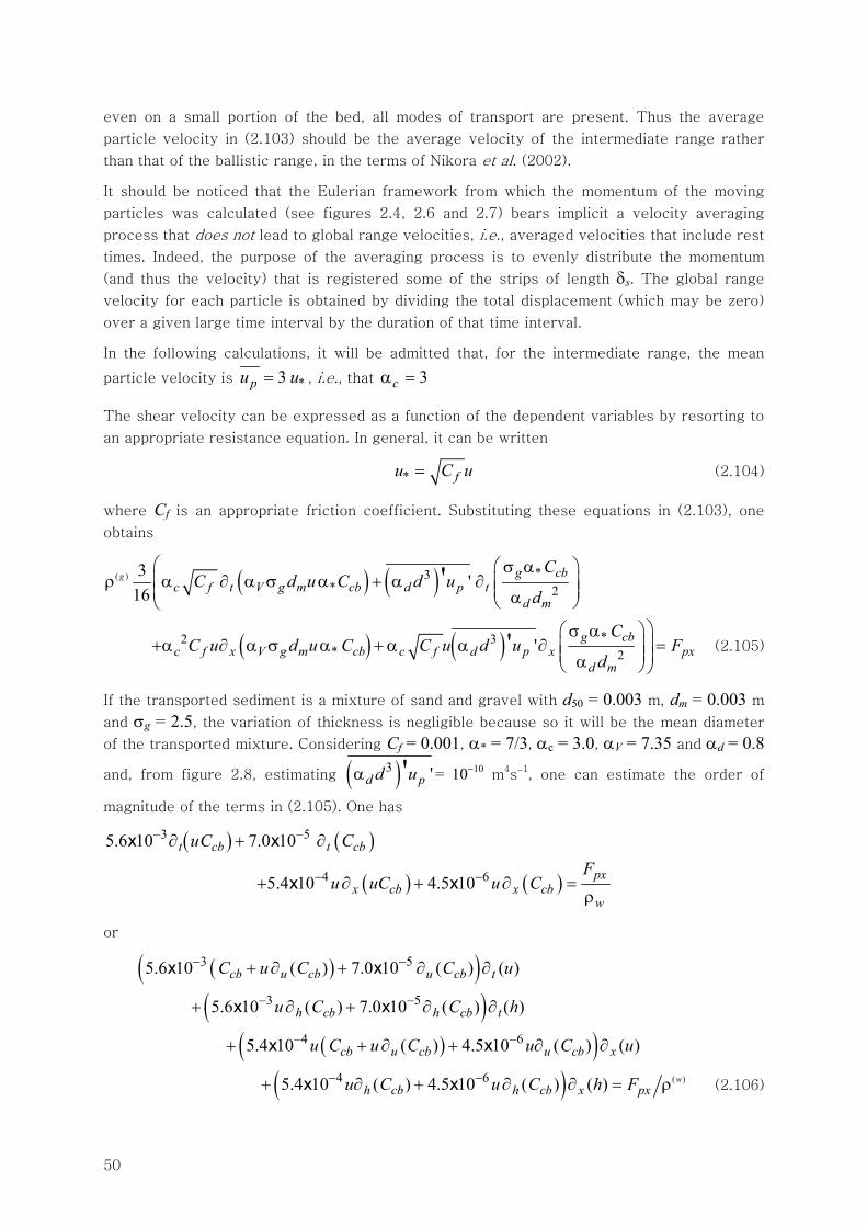
50

even on a small portion of the bed, all modes of transport are present. Thus the average

particle velocity in (2.103) should be the average velocity of the intermediate range rather

than that of the ballistic range, in the terms of Nikora et al. (2002).

It should be noticed that the Eulerian framework from which the momentum of the moving

particles was calculated (see figures 2.4, 2.6 and 2.7) bears implicit a velocity averaging

process that does not lead to global range velocities, i.e., averaged velocities that include rest

times. Indeed, the purpose of the averaging process is to evenly distribute the momentum

(and thus the velocity) that is registered some of the strips of length δs. The global range

velocity for each particle is obtained by dividing the total displacement (which may be zero)

over a given large time interval by the duration of that time interval.

In the following calculations, it will be admitted that, for the intermediate range, the mean

particle velocity is *3pu u= , i.e., that 3cα =

The shear velocity can be expressed as a function of the dependent variables by resorting to

an appropriate resistance equation. In general, it can be written

* fu C u= (2.104)

where Cf is an appropriate friction coefficient. Substituting these equations in (2.103), one

obtains

( ) ( )( ) *3* 2

3 ' 16

'g g cbc f t V g m cb d p t

d m

CC d u C d u

d

⎛ ⎛ ⎞σ α⎜ρ α ∂ α σ α + α ∂ ⎜ ⎟⎜ ⎟⎜ α⎝ ⎠⎝

( ) ( ) *2 3* 2'' g cb

c f x V g m cb c f d p x pxd m

CC u d u C C u d u F

d

⎞⎛ ⎞σ α⎟+α ∂ α σ α + α α ∂ =⎜ ⎟⎜ ⎟⎟α⎝ ⎠⎠

(2.105)

If the transported sediment is a mixture of sand and gravel with d50 = 0.003 m, dm = 0.003 m

and σg = 2.5, the variation of thickness is negligible because so it will be the mean diameter

of the transported mixture. Considering Cf = 0.001, α* = 7/3, αc = 3.0, αV = 7.35 and αd = 0.8

and, from figure 2.8, estimating ( )3 ''d pd uα = 10−10 m4s−1, one can estimate the order of

magnitude of the terms in (2.105). One has

( ) ( )3 55.6 10 7.0 10 t cb t cbuC C− −∂ + ∂x x

( ) ( )4 65.4 10 4.5 10 pxx cb x cb

w

Fu uC u C− −+ ∂ + ∂ =

ρx x

or

( )( )( )

( )( )( ) ( )

3 5

3 5

4 6

4 6

5.6 10 ( ) 7.0 10 ( ) ( )

5.6 10 ( ) 7.0 10 ( ) ( )

5.4 10 ( ) 4.5 10 ( ) ( )

5.4 10 ( ) 4.5 10 ( ) ( ) w

cb u cb u cb t

h cb h cb t

cb u cb u cb x

h cb h cb x px

C u C C u

u C C h

u C u C u C u

u C u C h F

− −

− −

− −

− −

+ ∂ + ∂ ∂

+ ∂ + ∂ ∂

+ + ∂ + ∂ ∂

+ ∂ + ∂ ∂ = ρ

x x

x x

x x

x x

(2.106)

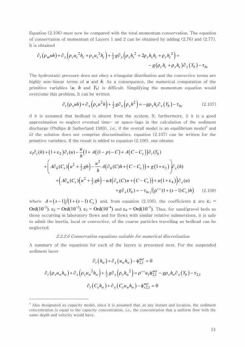
51

Equation (2.106) must now be compared with the total momentum conservation. The equation

of conservation of momentum of Layers 1 and 2 can be obtained by adding (2.76) and (2.77).

It is obtained

( ) ( ) ( )

( ) ( )

2 2 2 212 2

t m x c c c s s s x s s s s c c c

c c s s x b bc

uh u h u h g h h h h

g h h Y

∂ ρ + ∂ ρ + ρ + ∂ ρ + ρ + ρ =

− ρ + ρ ∂ − τ

The hydrostatic pressure does not obey a triangular distribution and the convective terms are

highly non-linear terms of u and h. As a consequence, the numerical computation of the

primitive variables (u, h and Yb) is difficult. Simplifying the momentum equation would

overcome this problem. It can be written

( ) ( ) ( ) ( )2 212t s x s x s s s x b bcuh u h g h g h Y∂ ρ + ∂ ρ + ∂ ρ = − ρ ∂ − τ (2.107)

if it is assumed that bedload is absent from the system. If, furthermore, i) it is a good

approximation to neglect eventual time- or space-lags in the calculation of the sediment

discharge (Phillips & Sutherland 1989), i.e., if the overall model is an equilibrium model4 and

ii) the solution does not comprise discontinuities, equation (2.107) can be written for the

primitive variables. If the result is added to equation (2.106), one obtains

( ) ( ) ( )( )1 2( ) 1 ( ) 1 (1 ) ( )t t s t buh u A p C A C C Yh

ε ∂ + + ε ∂ − + − − + − ∂

( ) ( )( ) ( )2

2 132( ) ( ) 1 ( )h s h s x

uA C u gh A C h C C g hh

⎛ ⎞+ ∂ + − ∂ + − + + ε ∂⎜ ⎟⎜ ⎟⎝ ⎠

( ) ( )( ) ( )( )2 142( ) ( ) 1 ( )u s u s xA C u gh uA C u C C u u+ ∂ + − ∂ + − + + ε ∂

( )( )( ) (1 ( 1) )wx b bc sg Y s C h+ ∂ = −τ ρ + − (2.108)

where ( ) ( )1 1 ( 1) sA s s C= − + − and, from equation (2.106), the coefficients ε are ε1 = Ord(10−2), ε2 = Ord(10−2), ε3 = Ord(10−4) and ε4 = Ord(10−5). Thus, for sand/gravel beds as

those occurring in laboratory flows and for flows with similar relative submersions, it is safe

to admit the inertia, local or convective, of the coarse particles travelling as bedload can be

neglected.

2.2.2.6 Conservation equations suitable for numerical discretization

A summary of the equations for each of the layers is presented next. For the suspended

sediment layer

( ) ( ) 2,1 0nett w x w wh u h∂ + ∂ − φ =

( ) ( ) ( ) ( )( )2 212,1 2,12

w nett s w w x s w w x s w I s w x bu h u h g h u g h Y∂ ρ + ∂ ρ + ∂ ρ = ρ φ − ρ ∂ − τ

( ) ( ) 2,1 0nett s w x s w w sC h C u h∂ + ∂ − φ =

4 Also designated as capacity model, since it is assumed that, at any instant and location, the sediment

concentration is equal to the capacity concentration, i.e., the concentration that a uniform flow with the

same depth and velocity would have.

52

In this text the situations of most practical interest are those for which the morphologic

impacts stem from the transport of sand and gravel. Thus, the importance of suspended

sediment in the bedload layer is limited, because the thickness of this layer is small

comparatively to the flow depth. Therefore, it will be assumed that b cbC C≈ and the

conservation equations are

( ) ( ) 2,1 3,2 0net nett b x b bh u h∂ + ∂ + φ − φ =

( ) ( ) ( ) ( )2 212,12 2 w net

t b b b x b b b x s w b b b Iu h u h g h h h u∂ ρ + ∂ ρ + ∂ ρ + ρ = ρ φ ( ) 2,1 3,2b b x bg h Y− ρ ∂ + τ − τ

( ) ( )* 2,1 3,2 3,2 0net net nett b b x b b b s c sC h C u h∂ α + ∂ + φ − φ − φ =

In the hypothesis that the suspended sediment discharge in the bedload layer is negligible, it

is admitted that 2,1 3,2net nets sφ = φ , i.e., that any flux of fine sediment coming from the upper layer

is necessarily deposited in the bed. The equations of conservation of the bed are

( ) 3,2 0nett bY∂ + φ =

( ) 3,2 3,2(1 ) 0net nett b c sp Y− ∂ + φ + φ =

from which one deduces that ( )3,2 3,2 3,2 (1 )net net netc s pφ = φ + φ − . The transport of granulometric

mixtures requires a conservation equation for the mixing layer. It reads

( ) (1 )t aL p∂ − 3,2netc+φ 3,2

nets+φ 4,3

netc−φ 4,3 0net

s−φ =

The conservation of the mass of each size is

( )(1 ) t a kp L F− ∂ 3,2netc k+φ 3,2

nets k+φ 4,3

netc k−φ 4,3 0net

s k−φ = (2.109)

where Fk is the percentage of the size fraction k in the mixing layer. The subscripts k in the

vertical fluxes in equation (2.109) stands for that size fraction. Indeed, dealing with

granulometric mixtures requires the splitting of sediment mass conservation equations into its

basic constituents, the conservation equations for each size fraction. In the case of the

suspended sediment layer, the equations are

( ) ( ) 2,1 0k k k

nett s w x s w w sC h C u h∂ + ∂ − φ = (2.110)

It is assumed that all the size fractions are transported with the same velocity. The

suspension hypothesis is behind this assumption. Naturally, the following summation holds

( ) ( ) 2,1 0k k k

nett s w x s w w s

k k k

C h C u h∂ + ∂ − φ =∑ ∑ ∑

and

( ) ( )k ks w s w s s

k k

C h C h C C= ⇔ =∑ ∑ (2.111)

Obviously, the summation of the vertical fluxes must be equal to the total vertical flux:

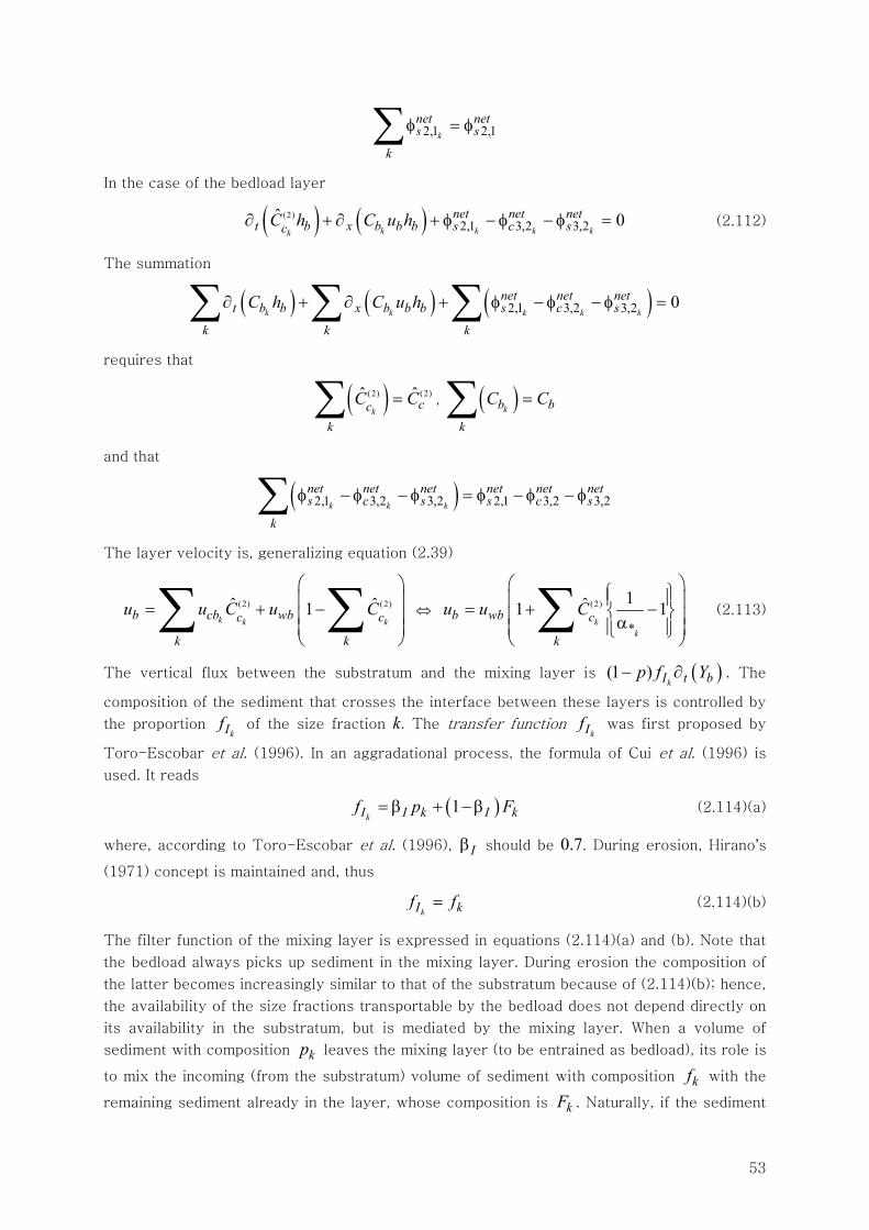
53

2,1 2,1k

net nets s

k

φ = φ∑

In the case of the bedload layer

( ) ( )(2)2,1 3,2 3,2

ˆ 0k k k kk

net net nett b x b b b s c scC h C u h∂ + ∂ + φ − φ − φ = (2.112)

The summation

( ) ( ) ( )2,1 3,2 3,2 0k k k k k

net net nett b b x b b b s c s

k k k

C h C u h∂ + ∂ + φ − φ − φ =∑ ∑ ∑

requires that

( )(2) (2)ˆ ˆk cc

k

C C=∑ , ( )kb b

k

C C=∑

and that

( )2,1 3,2 3,2 2,1 3,2 3,2k k k

net net net net net nets c s s c s

k

φ − φ − φ = φ − φ − φ∑

The layer velocity is, generalizing equation (2.39)

(2) (2)ˆ ˆ1

k k kb cb wbc c

k k

u u C u C⎛ ⎞⎜ ⎟= + −⎜ ⎟⎜ ⎟⎝ ⎠

∑ ∑ ⇔ (2)

*

1ˆ1 1k

k

b wb c

k

u u C⎛ ⎞⎧ ⎫⎪ ⎪⎜ ⎟= + −⎨ ⎬⎜ ⎟α⎪ ⎪⎜ ⎟⎩ ⎭⎝ ⎠∑ (2.113)

The vertical flux between the substratum and the mixing layer is ( )(1 )kI t bp f Y− ∂ . The

composition of the sediment that crosses the interface between these layers is controlled by

the proportion kIf of the size fraction k. The transfer function

kIf was first proposed by

Toro-Escobar et al. (1996). In an aggradational process, the formula of Cui et al. (1996) is

used. It reads

( )1kI I k I kf p F= β + −β (2.114)(a)

where, according to Toro-Escobar et al. (1996), Iβ should be 0.7. During erosion, Hirano’s

(1971) concept is maintained and, thus

kI kf f= (2.114)(b)

The filter function of the mixing layer is expressed in equations (2.114)(a) and (b). Note that

the bedload always picks up sediment in the mixing layer. During erosion the composition of

the latter becomes increasingly similar to that of the substratum because of (2.114)(b); hence,

the availability of the size fractions transportable by the bedload does not depend directly on

its availability in the substratum, but is mediated by the mixing layer. When a volume of

sediment with composition kp leaves the mixing layer (to be entrained as bedload), its role is

to mix the incoming (from the substratum) volume of sediment with composition kf with the

remaining sediment already in the layer, whose composition is kF . Naturally, if the sediment

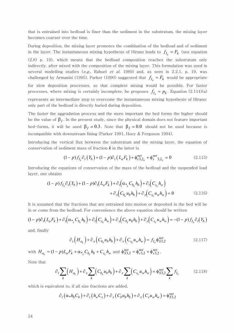
54

that is entrained into bedload is finer than the sediment in the substratum, the mixing layer

becomes coarser over the time.

During deposition, the mixing layer promotes the combination of the bedload and of sediment

in the layer. The instantaneous mixing hypothesis of Hirano leads to kI kf F= (see equation

(2.8) p. 19), which means that the bedload composition reaches the substratum only

indirectly, after mixed with the composition of the mixing layer. This formulation was used in

several modelling studies (e.g., Rahuel et al. 1989) and, as seen in 2.2.1, p. 19, was

challenged by Armanini (1995). Parker (1990) suggested that kI kf F= would be appropriate

for slow deposition processes, so that complete mixing would be possible. For faster

processes, where mixing is certainly incomplete, he proposes kI kf p= . Equation (2.114)(a)

represents an intermediate step to overcome the instantaneous mixing hypothesis of Hirano:

only part of the bedload is directly buried during deposition.

The faster the aggradation process and the more important the bed forms the higher should

be the value of Iβ . In the present study, since the physical domain does not feature important

bed-forms, it will be used 0.3Iβ = . Note that 0.0Iβ = should not be used because is

incompatible with downstream fining (Parker 1991, Hoey & Ferguson 1994).

Introducing the vertical flux between the substratum and the mixing layer, the equation of

conservation of sediment mass of fraction k in the latter is

( ) ( ) 3,2 3,2(1 ) (1 ) 0k k k

net netI t b t a k c sp f Y p L F− ∂ + − ∂ + φ + φ = (2.115)

Introducing the equations of conservation of the mass of the bedload and the suspended load

layer, one obtains

( ) ( ) ( ) ( )

( ) ( )*(1 ) (1 )

0

k k k k

k k

I t b t a k t b b t s w

x b b b x s w w

p f Y p L F C h C h

C u h C u h

− ∂ + − ∂ + ∂ α + ∂

+ ∂ + ∂ =

(2.116)

It is assumed that the fractions that are entrained into motion or deposited in the bed will be

in or come from the bedload. For convenience the above equation should be written

( ) ( ) ( ) ( ) ( ) ( )*(1 ) (1 )k k k k k kt a k t b b t s w x b b b x s w w I t bp L F C h C h C u h C u h p f Y− ∂ + ∂ α + ∂ + ∂ + ∂ = − − ∂

and, finally

( ) ( ) ( ) 3,2k k k k

nett a x b b b x s w w I SH C u h C u h f∂ + ∂ + ∂ = φ (2.117)

with *(1 )k k k ka a k b b s wH p L F C h C h= − + α + and 3,2 3,2 3,2

net net netS c sφ = φ + φ .

Note that

( ) ( ) ( ) 3,2k k k k

nett a x b b b x s w w S I

k k k k

H C u h C u h f∂ + ∂ + ∂ = φ∑ ∑ ∑ ∑ (2.118)

which is equivalent to, if all size fractions are added,

( ) ( ) ( ) ( )* 3,2net

t b b t w s x b b b x s w w Sh C h C C u h C u h∂ α + ∂ + ∂ + ∂ = φ

55

Note also that the proper way to compute Fk is

*

(1 )k k k ka b b s w

ka

H C h C hF

p L− α −

=−

(2.119)

and, thus,

*1

(1 ) kk a b b s wak k

F H C h C hp L

⎡ ⎤⎢ ⎥= − α −

− ⎢ ⎥⎣ ⎦∑ ∑ (2.120)

can be used to access numerical errors.

For convenience of computation, the water conservation equations are merged to obtain

( ) ( ) 0t b xh Y uh∂ + + ∂ = (2.121)

Likewise, the momentum equations become

( ) ( ) ( )( ) ( )

2 2 2 212 2

t m x b b b s w w x s w s w b b b

b b s w x b b

uh u h u h g h h h h

g h h Y

∂ ρ + ∂ ρ + ρ + ∂ ρ + ρ + ρ =

− ρ + ρ ∂ − τ

(2.122)

where 3,2bτ ≡ τ . Thus the final set of equations for the non-equilibrium model is

( ) ( ) 0t xY uh∂ + ∂ =

( ) ( ) ( )

( ) ( )

2 2 2 212 2

t x b b b s w w x s w s w b b b

b b s w x b b

R u h u h g h h h h

g h h Y

∂ + ∂ ρ + ρ + ∂ ρ + ρ + ρ =

− ρ + ρ ∂ − τ

(2.123)

( ) ( ) 2,1k k k

nett s w x s w w sC h C u h∂ + ∂ = φ (2.124)

( ) ( )* 2,1 3,2 3,2k k k k k k k

net net nett b b x b b b s c sC h C u h∂ α + ∂ = −φ + φ + φ (2.125)

( ) ( ) ( ) 3,2k k k k

nett a x c b b x s w w I SH C u h C u h f∂ + ∂ + ∂ = φ (2.126)

( ) 3,2(1 ) 0nett b Sp Y− ∂ + φ = (2.127)

The conservative variables are bY h Y= + , mR uh= ρ , k ks s wH C h= , *k k kb b bH C h= α and

*(1 )k k k ka a k b b s wH p L F C h C h= − + α + .

For the equilibrium model, neglecting the contribution of the inertia of the coarse particles

(see equation (2.108)), the conservative formulation is

( )( ) 0t xY uh∂ + ∂ = (2.128)

( )2 212( ) ( )t s x s s s x b bR u h gh gh Y∂ + ∂ ρ + ρ = −ρ ∂ − τ (2.129)

( )( ) 0t xZ C uh∂ + ∂ = (2.130)

Equations (2.128) to (2.130) express, respectively, the total mass conservation, the

conservation of momentum and the sediment mass conservation. The system of equations is

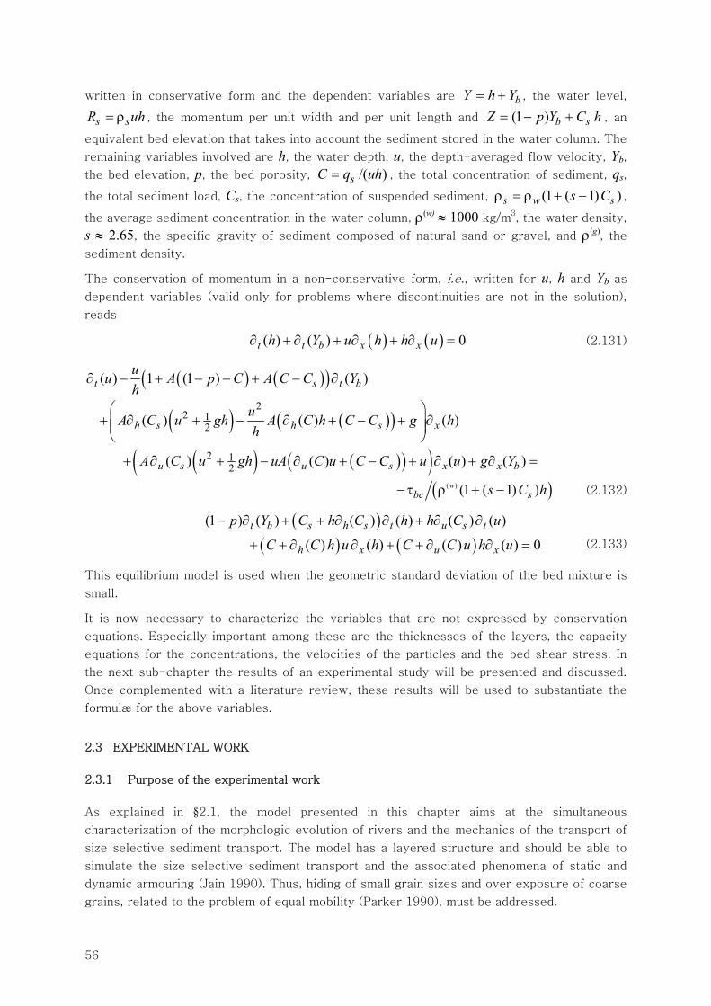
56

written in conservative form and the dependent variables are bY h Y= + , the water level,

s sR uh= ρ , the momentum per unit width and per unit length and (1 ) b sZ p Y C h= − + , an

equivalent bed elevation that takes into account the sediment stored in the water column. The

remaining variables involved are h, the water depth, u, the depth-averaged flow velocity, Yb,

the bed elevation, p, the bed porosity, /( )sC q uh= , the total concentration of sediment, qs,

the total sediment load, Cs, the concentration of suspended sediment, (1 ( 1) )s w ss Cρ = ρ + − ,

the average sediment concentration in the water column, ρ(w) ≈ 1000 kg/m3, the water density,

s ≈ 2.65, the specific gravity of sediment composed of natural sand or gravel, and ρ(g), the

sediment density.

The conservation of momentum in a non-conservative form, i.e., written for u, h and Yb as

dependent variables (valid only for problems where discontinuities are not in the solution),

reads

( ) ( )( ) ( ) 0t t b x xh Y u h h u∂ + ∂ + ∂ + ∂ = (2.131)

( ) ( )( )( ) 1 (1 ) ( )t s t buu A p C A C C Yh

∂ − + − − + − ∂

( ) ( )( )2

2 12( ) ( ) ( )h s h s x

uA C u gh A C h C C g hh

⎛ ⎞+ ∂ + − ∂ + − + ∂⎜ ⎟⎜ ⎟⎝ ⎠

( ) ( )( )( )2 12( ) ( ) ( ) ( )u s u s x x bA C u gh uA C u C C u u g Y+ ∂ + − ∂ + − + ∂ + ∂ =

( )( ) (1 ( 1) )wbc ss C h−τ ρ + − (2.132)

( )

( ) ( )(1 ) ( ) ( ) ( ) ( ) ( )

( ) ( ) ( ) ( ) 0t b s h s t u s t

h x u x

p Y C h C h h C u

C C h u h C C u h u

− ∂ + + ∂ ∂ + ∂ ∂

+ + ∂ ∂ + + ∂ ∂ =

(2.133)

This equilibrium model is used when the geometric standard deviation of the bed mixture is

small.

It is now necessary to characterize the variables that are not expressed by conservation

equations. Especially important among these are the thicknesses of the layers, the capacity

equations for the concentrations, the velocities of the particles and the bed shear stress. In

the next sub-chapter the results of an experimental study will be presented and discussed.

Once complemented with a literature review, these results will be used to substantiate the

formulæ for the above variables.

2.3 EXPERIMENTAL WORK

2.3.1 Purpose of the experimental work

As explained in §2.1, the model presented in this chapter aims at the simultaneous

characterization of the morphologic evolution of rivers and the mechanics of the transport of

size selective sediment transport. The model has a layered structure and should be able to

simulate the size selective sediment transport and the associated phenomena of static and

dynamic armouring (Jain 1990). Thus, hiding of small grain sizes and over exposure of coarse

grains, related to the problem of equal mobility (Parker 1990), must be addressed.

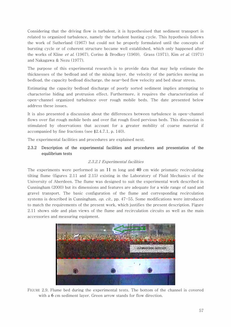
57

Considering that the driving flow is turbulent, it is hypothesised that sediment transport is

related to organized turbulence, namely the turbulent busting cycle. This hypothesis follows

the work of Sutherland (1967) but could not be properly formulated until the concepts of

bursting cycle or of coherent structure became well established, which only happened after

the works of Kline et al. (1967), Corino & Brodkey (1969), Grass (1971), Kim et al. (1971)

and Nakagawa & Nezu (1977).

The purpose of this experimental research is to provide data that may help estimate the

thicknesses of the bedload and of the mixing layer, the velocity of the particles moving as

bedload, the capacity bedload discharge, the near-bed flow velocity and bed shear stress.

Estimating the capacity bedload discharge of poorly sorted sediment implies attempting to

characterise hiding and protrusion effect. Furthermore, it requires the characterization of

open-channel organized turbulence over rough mobile beds. The date presented below

address these issues.

It is also presented a discussion about the differences between turbulence in open-channel

flows over flat rough mobile beds and over flat rough fixed pervious beds. This discussion is

stimulated by observations that account for a greater mobility of coarse material if

accompanied by fine fractions (see §2.4.7.1, p. 140).

The experimental facilities and procedures are explained next.

2.3.2 Description of the experimental facilities and procedures and presentation of the

equilibrium tests

2.3.2.1 Experimental facilities

The experiments were performed in an 11 m long and 40 cm wide prismatic recirculating

tilting flume (figures 2.11 and 2.15) existing in the Laboratory of Fluid Mechanics of the

University of Aberdeen. The flume was designed to suit the experimental work described in

Cunningham (2000) but its dimensions and features are adequate for a wide range of sand and

gravel transport. The basic configuration of the flume and corresponding recirculation

systems is described in Cunningham, op. cit., pp. 47-55. Some modifications were introduced

to match the requirements of the present work, which justifies the present description. Figure

2.11 shows side and plan views of the flume and recirculation circuits as well as the main

accessories and measuring equipment.

FIGURE 2.9. Flume bed during the experimental tests. The bottom of the channel is covered

with a 6 cm sediment layer. Green arrow stands for flow direction.

cohesionless sediment

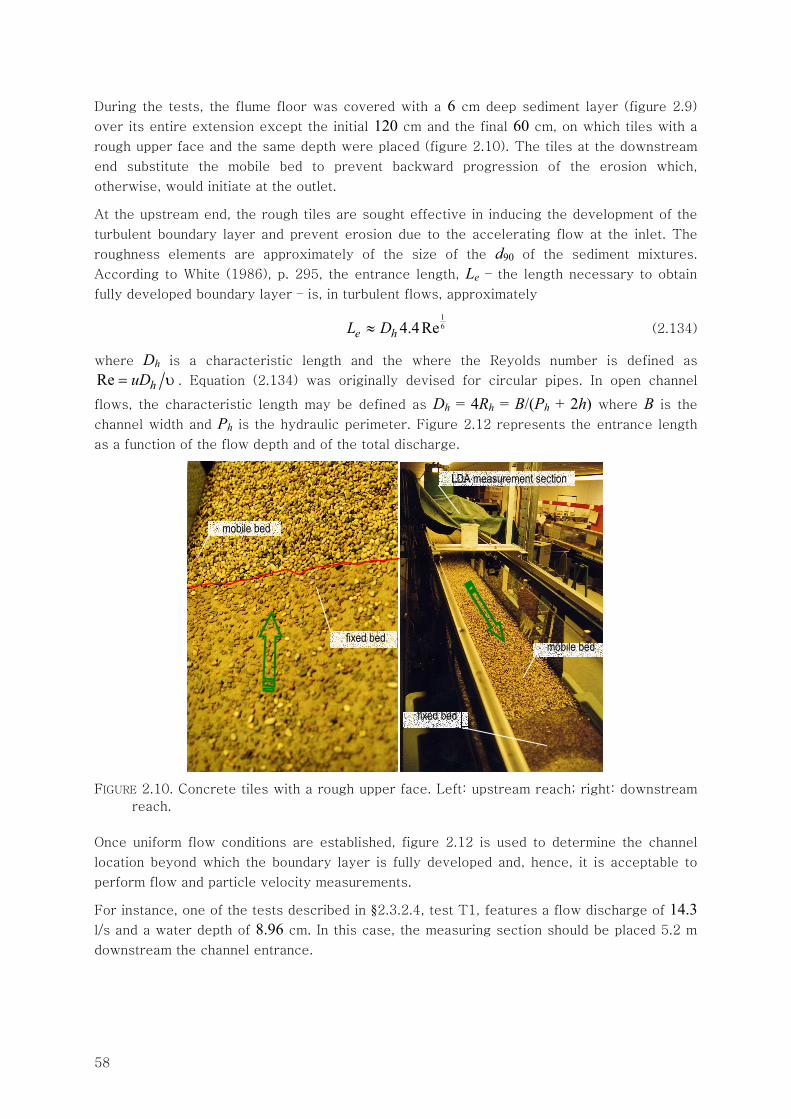
58

During the tests, the flume floor was covered with a 6 cm deep sediment layer (figure 2.9)

over its entire extension except the initial 120 cm and the final 60 cm, on which tiles with a

rough upper face and the same depth were placed (figure 2.10). The tiles at the downstream

end substitute the mobile bed to prevent backward progression of the erosion which,

otherwise, would initiate at the outlet.

At the upstream end, the rough tiles are sought effective in inducing the development of the

turbulent boundary layer and prevent erosion due to the accelerating flow at the inlet. The

roughness elements are approximately of the size of the d90 of the sediment mixtures.

According to White (1986), p. 295, the entrance length, Le – the length necessary to obtain

fully developed boundary layer – is, in turbulent flows, approximately

164.4 Ree hL D≈ (2.134)

where Dh is a characteristic length and the where the Reyolds number is defined as

Re huD= υ . Equation (2.134) was originally devised for circular pipes. In open channel

flows, the characteristic length may be defined as Dh = 4Rh = B/(Ph + 2h) where B is the

channel width and Ph is the hydraulic perimeter. Figure 2.12 represents the entrance length

as a function of the flow depth and of the total discharge.

FIGURE 2.10. Concrete tiles with a rough upper face. Left: upstream reach; right: downstream

reach.

Once uniform flow conditions are established, figure 2.12 is used to determine the channel

location beyond which the boundary layer is fully developed and, hence, it is acceptable to

perform flow and particle velocity measurements.

For instance, one of the tests described in §2.3.2.4, test T1, features a flow discharge of 14.3

l/s and a water depth of 8.96 cm. In this case, the measuring section should be placed 5.2 m

downstream the channel entrance.

fixed bed

mobile bed

LDA measurement section

mobile bed

fixed bed

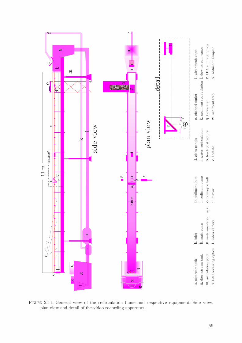
59

FIGURE 2.11. General view of the recirculation flume and respective equipment. Side view,

plan view and detail of the video recording apparatus.

f. w

ire-m

esh c

one

l. d

ow

nstr

eam

vanes

r. L

DA

em

itting o

ptics

x. sedim

ent

sam

ple

r

e. channel outlet

k. sedim

ent

recir

cula

tion

q. flow

mete

r

w. sedim

ent

trap

d. gla

ss p

anels

j. w

ate

r re

cir

cula

tion

p. fe

edin

g s

tructu

re

v. aceta

te

b. sedim

ent

inle

t

i. s

edim

ent

pum

p

o. conveyor

belt

u. m

irro

r

b. in

let

h. m

ain

pum

p

n. in

str

um

enta

tion r

ails

t. v

ideo c

am

era

a. upstr

eam

tank

g. dow

nstr

eam

tank

m. art

icula

tion p

oin

t

s. LA

D r

eceiv

ing o

ptics

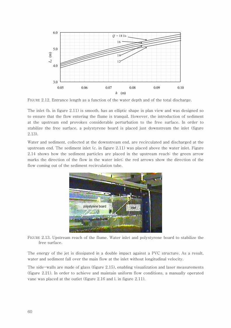
60

3.0

4.0

5.0

6.0

0.05 0.06 0.07 0.08 0.09 0.10h (m)

L e (

m)

Q = 18 l/s

16

14

12

FIGURE 2.12. Entrance length as a function of the water depth and of the total discharge.

The inlet (b. in figure 2.11) is smooth, has an elliptic shape in plan view and was designed so

to ensure that the flow entering the flume is tranquil. However, the introduction of sediment

at the upstream end provokes considerable perturbation to the free surface. In order to

stabilize the free surface, a polystyrene board is placed just downstream the inlet (figure

2.13).

Water and sediment, collected at the downstream end, are recirculated and discharged at the

upstream end. The sediment inlet (c. in figure 2.11) was placed above the water inlet. Figure

2.14 shows how the sediment particles are placed in the upstream reach: the green arrow

marks the direction of the flow in the water inlet; the red arrows show the direction of the

flow coming out of the sediment recirculation tube.

FIGURE 2.13. Upstream reach of the flume. Water inlet and polystyrene board to stabilize the

free surface.

The energy of the jet is dissipated in a double impact against a PVC structure. As a result,

water and sediment fall over the main flow at the inlet without longitudinal velocity.

The side-walls are made of glass (figure 2.15), enabling visualization and laser measurements

(figure 2.21). In order to achieve and maintain uniform flow conditions, a manually operated

vane was placed at the outlet (figure 2.16 and l. in figure 2.11).

polystyrene board inlet

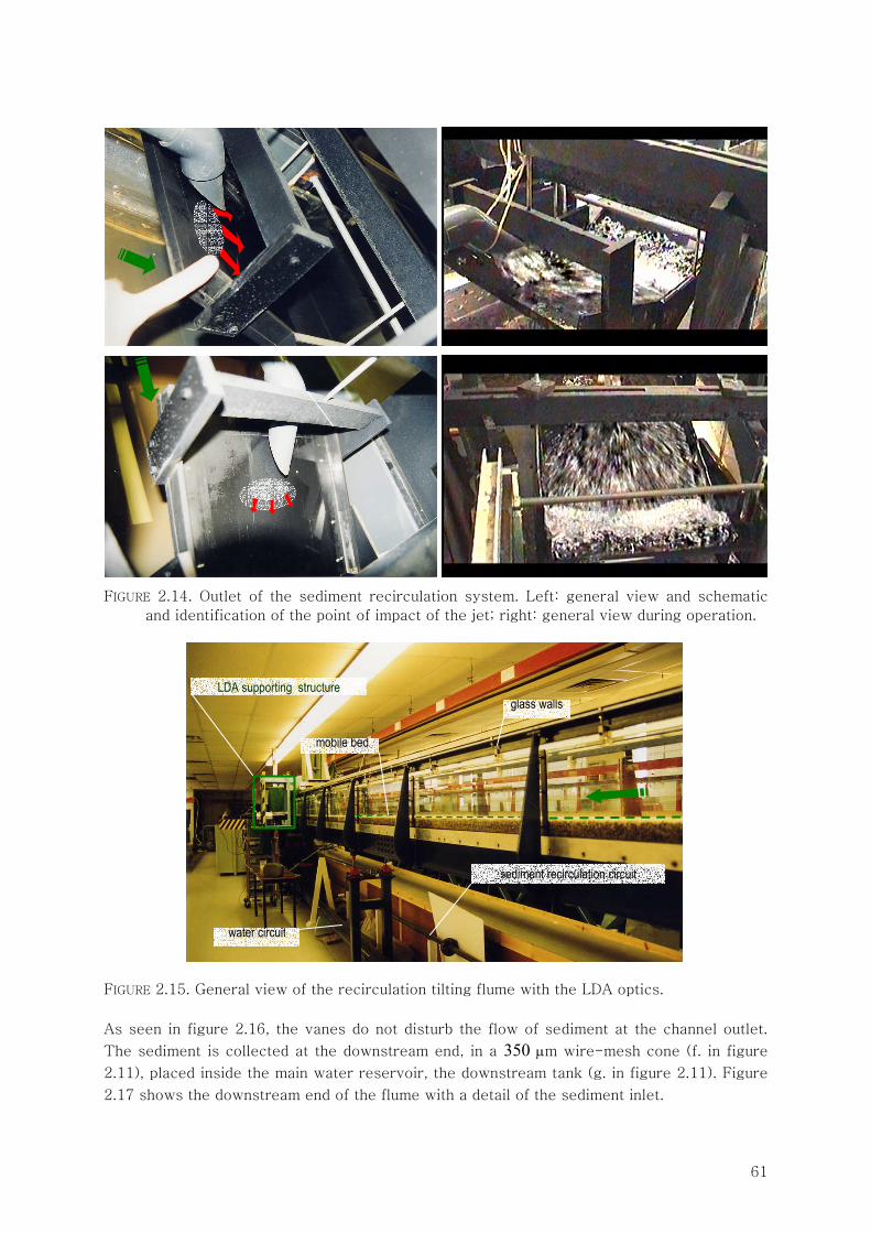
61

FIGURE 2.14. Outlet of the sediment recirculation system. Left: general view and schematic

and identification of the point of impact of the jet; right: general view during operation.

FIGURE 2.15. General view of the recirculation tilting flume with the LDA optics.

As seen in figure 2.16, the vanes do not disturb the flow of sediment at the channel outlet.

The sediment is collected at the downstream end, in a 350 μm wire-mesh cone (f. in figure

2.11), placed inside the main water reservoir, the downstream tank (g. in figure 2.11). Figure

2.17 shows the downstream end of the flume with a detail of the sediment inlet.

mobile bed

LDA supporting structure

sediment recirculation circuit

water circuit

glass walls

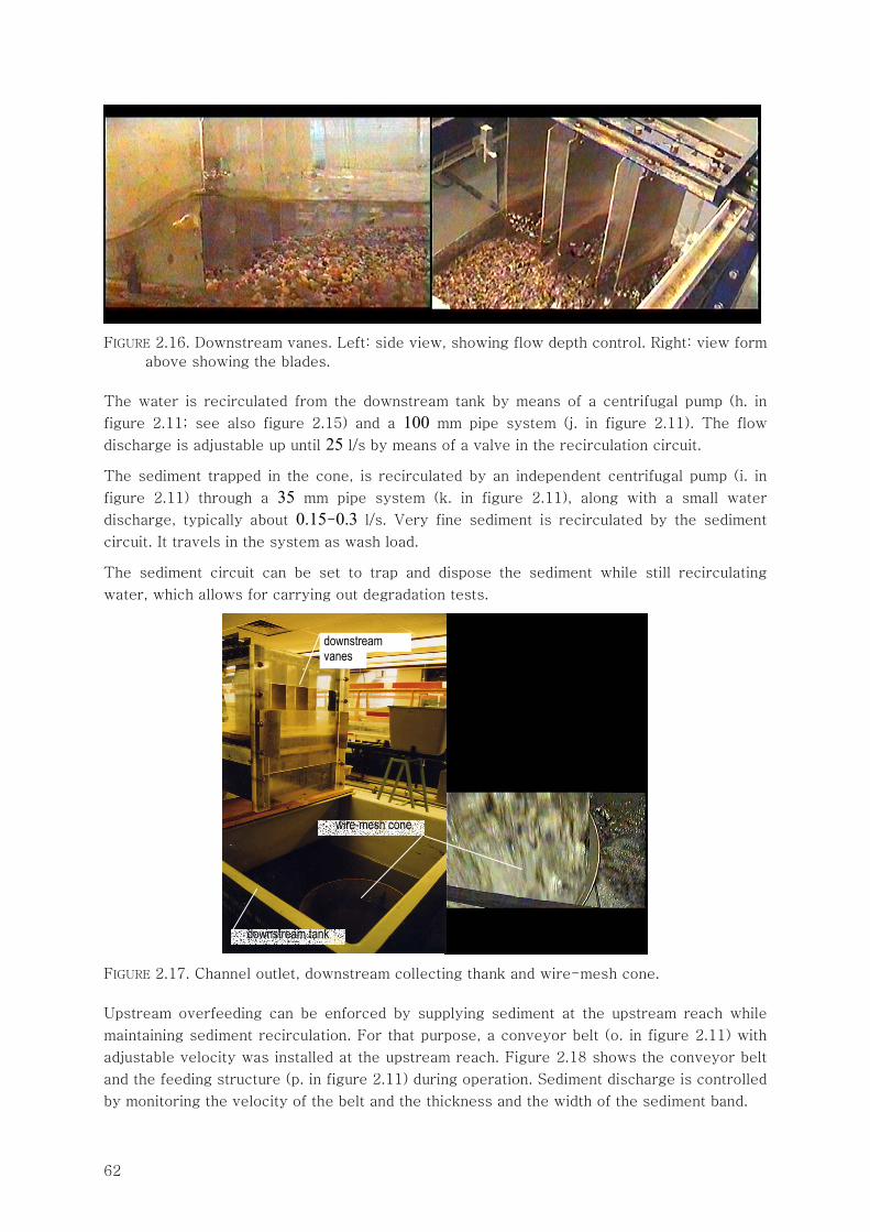
62

FIGURE 2.16. Downstream vanes. Left: side view, showing flow depth control. Right: view form

above showing the blades.

The water is recirculated from the downstream tank by means of a centrifugal pump (h. in

figure 2.11; see also figure 2.15) and a 100 mm pipe system (j. in figure 2.11). The flow

discharge is adjustable up until 25 l/s by means of a valve in the recirculation circuit.

The sediment trapped in the cone, is recirculated by an independent centrifugal pump (i. in

figure 2.11) through a 35 mm pipe system (k. in figure 2.11), along with a small water

discharge, typically about 0.15-0.3 l/s. Very fine sediment is recirculated by the sediment

circuit. It travels in the system as wash load.

The sediment circuit can be set to trap and dispose the sediment while still recirculating

water, which allows for carrying out degradation tests.

FIGURE 2.17. Channel outlet, downstream collecting thank and wire-mesh cone.

Upstream overfeeding can be enforced by supplying sediment at the upstream reach while

maintaining sediment recirculation. For that purpose, a conveyor belt (o. in figure 2.11) with

adjustable velocity was installed at the upstream reach. Figure 2.18 shows the conveyor belt

and the feeding structure (p. in figure 2.11) during operation. Sediment discharge is controlled

by monitoring the velocity of the belt and the thickness and the width of the sediment band.

downstream vanes

wire-mesh cone

downstream tank

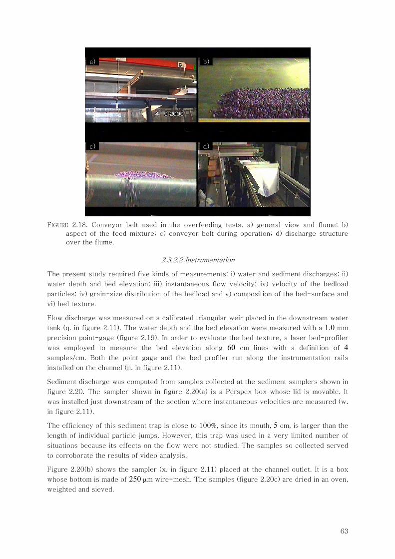
63

FIGURE 2.18. Conveyor belt used in the overfeeding tests. a) general view and flume; b)

aspect of the feed mixture; c) conveyor belt during operation; d) discharge structure

over the flume.

2.3.2.2 Instrumentation

The present study required five kinds of measurements: i) water and sediment discharges; ii)

water depth and bed elevation; iii) instantaneous flow velocity; iv) velocity of the bedload

particles; iv) grain-size distribution of the bedload and v) composition of the bed-surface and

vi) bed texture.

Flow discharge was measured on a calibrated triangular weir placed in the downstream water

tank (q. in figure 2.11). The water depth and the bed elevation were measured with a 1.0 mm

precision point-gage (figure 2.19). In order to evaluate the bed texture, a laser bed-profiler

was employed to measure the bed elevation along 60 cm lines with a definition of 4

samples/cm. Both the point gage and the bed profiler run along the instrumentation rails

installed on the channel (n. in figure 2.11).

Sediment discharge was computed from samples collected at the sediment samplers shown in

figure 2.20. The sampler shown in figure 2.20(a) is a Perspex box whose lid is movable. It

was installed just downstream of the section where instantaneous velocities are measured (w.

in figure 2.11).

The efficiency of this sediment trap is close to 100%, since its mouth, 5 cm, is larger than the

length of individual particle jumps. However, this trap was used in a very limited number of

situations because its effects on the flow were not studied. The samples so collected served

to corroborate the results of video analysis.

Figure 2.20(b) shows the sampler (x. in figure 2.11) placed at the channel outlet. It is a box

whose bottom is made of 250 μm wire-mesh. The samples (figure 2.20c) are dried in an oven,

weighted and sieved.

a) b)

c) d)

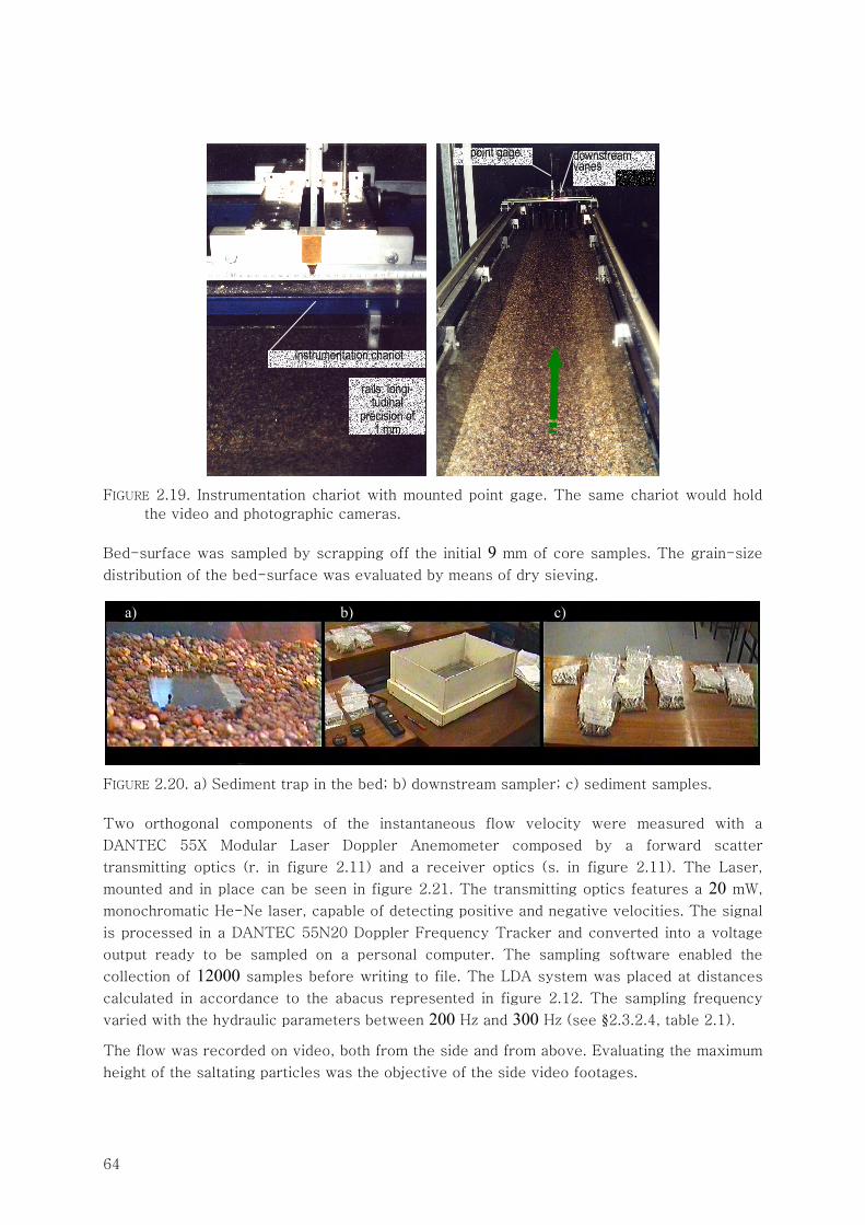
64

FIGURE 2.19. Instrumentation chariot with mounted point gage. The same chariot would hold

the video and photographic cameras.

Bed-surface was sampled by scrapping off the initial 9 mm of core samples. The grain-size

distribution of the bed-surface was evaluated by means of dry sieving.

FIGURE 2.20. a) Sediment trap in the bed; b) downstream sampler; c) sediment samples.

Two orthogonal components of the instantaneous flow velocity were measured with a

DANTEC 55X Modular Laser Doppler Anemometer composed by a forward scatter

transmitting optics (r. in figure 2.11) and a receiver optics (s. in figure 2.11). The Laser,

mounted and in place can be seen in figure 2.21. The transmitting optics features a 20 mW,

monochromatic He-Ne laser, capable of detecting positive and negative velocities. The signal

is processed in a DANTEC 55N20 Doppler Frequency Tracker and converted into a voltage

output ready to be sampled on a personal computer. The sampling software enabled the

collection of 12000 samples before writing to file. The LDA system was placed at distances

calculated in accordance to the abacus represented in figure 2.12. The sampling frequency

varied with the hydraulic parameters between 200 Hz and 300 Hz (see §2.3.2.4, table 2.1).

The flow was recorded on video, both from the side and from above. Evaluating the maximum

height of the saltating particles was the objective of the side video footages.

downstream vanes

point gage

instrumentation chariot

rails: longi-tudinal

precision of 1 mm

a) b) c)

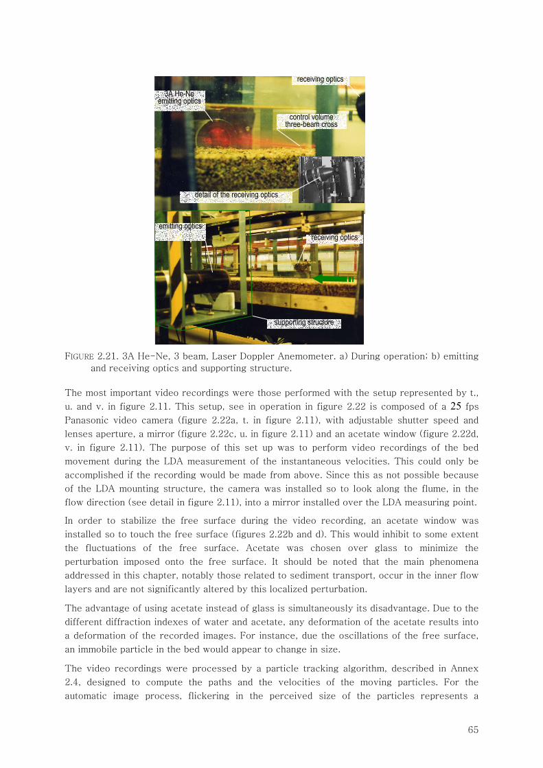
65

FIGURE 2.21. 3A He-Ne, 3 beam, Laser Doppler Anemometer. a) During operation; b) emitting

and receiving optics and supporting structure.

The most important video recordings were those performed with the setup represented by t.,

u. and v. in figure 2.11. This setup, see in operation in figure 2.22 is composed of a 25 fps

Panasonic video camera (figure 2.22a, t. in figure 2.11), with adjustable shutter speed and

lenses aperture, a mirror (figure 2.22c, u. in figure 2.11) and an acetate window (figure 2.22d,

v. in figure 2.11). The purpose of this set up was to perform video recordings of the bed

movement during the LDA measurement of the instantaneous velocities. This could only be

accomplished if the recording would be made from above. Since this as not possible because

of the LDA mounting structure, the camera was installed so to look along the flume, in the

flow direction (see detail in figure 2.11), into a mirror installed over the LDA measuring point.

In order to stabilize the free surface during the video recording, an acetate window was

installed so to touch the free surface (figures 2.22b and d). This would inhibit to some extent

the fluctuations of the free surface. Acetate was chosen over glass to minimize the

perturbation imposed onto the free surface. It should be noted that the main phenomena

addressed in this chapter, notably those related to sediment transport, occur in the inner flow

layers and are not significantly altered by this localized perturbation.

The advantage of using acetate instead of glass is simultaneously its disadvantage. Due to the

different diffraction indexes of water and acetate, any deformation of the acetate results into

a deformation of the recorded images. For instance, due the oscillations of the free surface,

an immobile particle in the bed would appear to change in size.

The video recordings were processed by a particle tracking algorithm, described in Annex

2.4, designed to compute the paths and the velocities of the moving particles. For the

automatic image process, flickering in the perceived size of the particles represents a

3A He-Ne emitting optics

receiving optics

control volume three-beam cross

supporting structure

emitting optics receiving optics

detail of the receiving optics

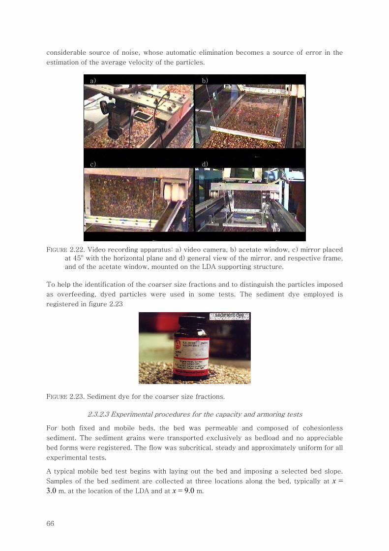
66

considerable source of noise, whose automatic elimination becomes a source of error in the

estimation of the average velocity of the particles.

FIGURE 2.22. Video recording apparatus: a) video camera, b) acetate window, c) mirror placed

at 45o with the horizontal plane and d) general view of the mirror, and respective frame,

and of the acetate window, mounted on the LDA supporting structure.

To help the identification of the coarser size fractions and to distinguish the particles imposed

as overfeeding, dyed particles were used in some tests. The sediment dye employed is

registered in figure 2.23

FIGURE 2.23. Sediment dye for the coarser size fractions.

2.3.2.3 Experimental procedures for the capacity and armoring tests

For both fixed and mobile beds, the bed was permeable and composed of cohesionless

sediment. The sediment grains were transported exclusively as bedload and no appreciable

bed forms were registered. The flow was subcritical, steady and approximately uniform for all

experimental tests.

A typical mobile bed test begins with laying out the bed and imposing a selected bed slope.

Samples of the bed sediment are collected at three locations along the bed, typically at x = 3.0 m, at the location of the LDA and at x = 9.0 m.

sediment dye

a) b)

c) d)

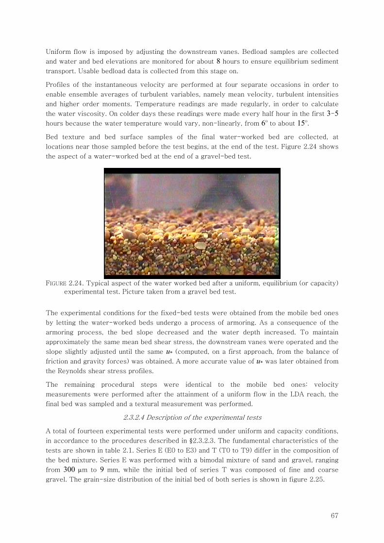
67

Uniform flow is imposed by adjusting the downstream vanes. Bedload samples are collected

and water and bed elevations are monitored for about 8 hours to ensure equilibrium sediment

transport. Usable bedload data is collected from this stage on.

Profiles of the instantaneous velocity are performed at four separate occasions in order to

enable ensemble averages of turbulent variables, namely mean velocity, turbulent intensities

and higher order moments. Temperature readings are made regularly, in order to calculate

the water viscosity. On colder days these readings were made every half hour in the first 3-5

hours because the water temperature would vary, non-linearly, from 6o to about 15o.

Bed texture and bed surface samples of the final water-worked bed are collected, at

locations near those sampled before the test begins, at the end of the test. Figure 2.24 shows

the aspect of a water-worked bed at the end of a gravel-bed test.

FIGURE 2.24. Typical aspect of the water worked bed after a uniform, equilibrium (or capacity)

experimental test. Picture taken from a gravel bed test.

The experimental conditions for the fixed-bed tests were obtained from the mobile bed ones

by letting the water-worked beds undergo a process of armoring. As a consequence of the

armoring process, the bed slope decreased and the water depth increased. To maintain

approximately the same mean bed shear stress, the downstream vanes were operated and the

slope slightly adjusted until the same u* (computed, on a first approach, from the balance of

friction and gravity forces) was obtained. A more accurate value of u* was later obtained from

the Reynolds shear stress profiles.

The remaining procedural steps were identical to the mobile bed ones: velocity

measurements were performed after the attainment of a uniform flow in the LDA reach, the

final bed was sampled and a textural measurement was performed.

2.3.2.4 Description of the experimental tests

A total of fourteen experimental tests were performed under uniform and capacity conditions,

in accordance to the procedures described in §2.3.2.3. The fundamental characteristics of the

tests are shown in table 2.1. Series E (E0 to E3) and T (T0 to T9) differ in the composition of

the bed mixture. Series E was performed with a bimodal mixture of sand and gravel, ranging

from 300 μm to 9 mm, while the initial bed of series T was composed of fine and coarse

gravel. The grain-size distribution of the initial bed of both series is shown in figure 2.25.

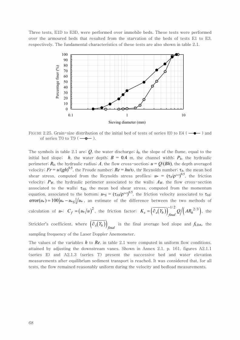
68

Three tests, E1D to E3D, were performed over immobile beds. These tests were performed

over the armoured beds that resulted from the starvation of the beds of tests E1 to E3,

respectively. The fundamental characteristics of these tests are also shown in table 2.1.

0102030405060708090

100

0.1 1 10

Sieving diameter (mm)

Perc

enta

ge fi

ner (

%)

FIGURE 2.25. Grain-size distribution of the initial bed of tests of series E0 to E4 ( ) and

of series T0 to T9 ( ).

The symbols in table 2.1 are: Q, the water discharge; i0, the slope of the flume, equal to the

initial bed slope; h, the water depth; B = 0.4 m, the channel width; Ph, the hydraulic

perimeter; Rh, the hydraulic radius; A, the flow cross-section; u = Q/(Bh), the depth averaged

velocity; Fr = u/(gh)0.5, the Froude number; Re = hu/υ, thr Reynolds number; τb, the mean bed

shear stress, computed from the Reynolds stress profiles; u* = (τb/ρ(w))0.5, the friction

velocity; PW, the hydraulic perimeter associated to the walls; AW, the flow cross-section

associated to the walls; τbS, the mean bed shear stress, computed from the momentum

equation, associated to the bottom; u*S = (τbS/ρ(w))0.5, the friction velocity associated to τbS;

* * * *error( ) 100 Su u u u= − , an estimate of the difference between the two methods of

calculation of u*; ( )2*fC u u= , the friction factor; ( )( ) ( )1/ 2 2 / 3

s x b hfinalK Y Q AR

−= ∂ , the

Strickler’s coefficient, where ( )( )x b finalY∂ is the final average bed slope and fLDA, the

sampling frequency of the Laser Doppler Anemometer.

The values of the variables h to Re, in table 2.1 were computed in uniform flow conditions,

attained by adjusting the downstream vanes. Shown in Annex 2.1, p. 161, figures A2.1.1

(series E) and A2.1.3 (series T) present the successive bed and water elevation

measurements after equilibrium sediment transport is reached. It was considered that, for all

tests, the flow remained reasonably uniform during the velocity and bedload measurements.

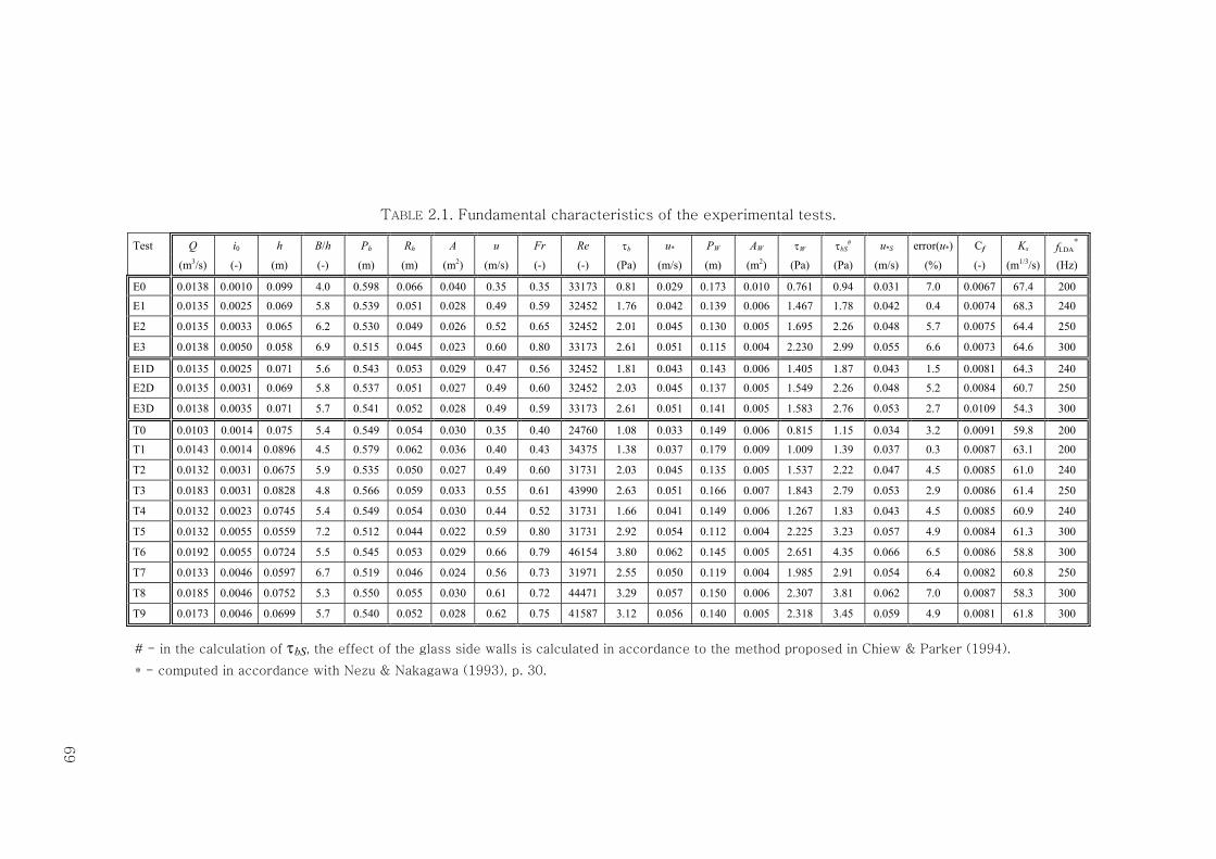
69

TABLE 2.1. Fundamental characteristics of the experimental tests.

Test Q i0 h B/h Ph Rh A u Fr Re τb u* PW AW τW τbS# u*S error(u*) Cf Ks fLDA

* (m3/s) (-) (m) (-) (m) (m) (m2) (m/s) (-) (-) (Pa) (m/s) (m) (m2) (Pa) (Pa) (m/s) (%) (-) (m1/3/s) (Hz)

E0 0.0138 0.0010 0.099 4.0 0.598 0.066 0.040 0.35 0.35 33173 0.81 0.029 0.173 0.010 0.761 0.94 0.031 7.0 0.0067 67.4 200

E1 0.0135 0.0025 0.069 5.8 0.539 0.051 0.028 0.49 0.59 32452 1.76 0.042 0.139 0.006 1.467 1.78 0.042 0.4 0.0074 68.3 240

E2 0.0135 0.0033 0.065 6.2 0.530 0.049 0.026 0.52 0.65 32452 2.01 0.045 0.130 0.005 1.695 2.26 0.048 5.7 0.0075 64.4 250

E3 0.0138 0.0050 0.058 6.9 0.515 0.045 0.023 0.60 0.80 33173 2.61 0.051 0.115 0.004 2.230 2.99 0.055 6.6 0.0073 64.6 300

E1D 0.0135 0.0025 0.071 5.6 0.543 0.053 0.029 0.47 0.56 32452 1.81 0.043 0.143 0.006 1.405 1.87 0.043 1.5 0.0081 64.3 240

E2D 0.0135 0.0031 0.069 5.8 0.537 0.051 0.027 0.49 0.60 32452 2.03 0.045 0.137 0.005 1.549 2.26 0.048 5.2 0.0084 60.7 250

E3D 0.0138 0.0035 0.071 5.7 0.541 0.052 0.028 0.49 0.59 33173 2.61 0.051 0.141 0.005 1.583 2.76 0.053 2.7 0.0109 54.3 300

T0 0.0103 0.0014 0.075 5.4 0.549 0.054 0.030 0.35 0.40 24760 1.08 0.033 0.149 0.006 0.815 1.15 0.034 3.2 0.0091 59.8 200

T1 0.0143 0.0014 0.0896 4.5 0.579 0.062 0.036 0.40 0.43 34375 1.38 0.037 0.179 0.009 1.009 1.39 0.037 0.3 0.0087 63.1 200

T2 0.0132 0.0031 0.0675 5.9 0.535 0.050 0.027 0.49 0.60 31731 2.03 0.045 0.135 0.005 1.537 2.22 0.047 4.5 0.0085 61.0 240

T3 0.0183 0.0031 0.0828 4.8 0.566 0.059 0.033 0.55 0.61 43990 2.63 0.051 0.166 0.007 1.843 2.79 0.053 2.9 0.0086 61.4 250

T4 0.0132 0.0023 0.0745 5.4 0.549 0.054 0.030 0.44 0.52 31731 1.66 0.041 0.149 0.006 1.267 1.83 0.043 4.5 0.0085 60.9 240

T5 0.0132 0.0055 0.0559 7.2 0.512 0.044 0.022 0.59 0.80 31731 2.92 0.054 0.112 0.004 2.225 3.23 0.057 4.9 0.0084 61.3 300

T6 0.0192 0.0055 0.0724 5.5 0.545 0.053 0.029 0.66 0.79 46154 3.80 0.062 0.145 0.005 2.651 4.35 0.066 6.5 0.0086 58.8 300

T7 0.0133 0.0046 0.0597 6.7 0.519 0.046 0.024 0.56 0.73 31971 2.55 0.050 0.119 0.004 1.985 2.91 0.054 6.4 0.0082 60.8 250

T8 0.0185 0.0046 0.0752 5.3 0.550 0.055 0.030 0.61 0.72 44471 3.29 0.057 0.150 0.006 2.307 3.81 0.062 7.0 0.0087 58.3 300

T9 0.0173 0.0046 0.0699 5.7 0.540 0.052 0.028 0.62 0.75 41587 3.12 0.056 0.140 0.005 2.318 3.45 0.059 4.9 0.0081 61.8 300

# - in the calculation of τbS, the effect of the glass side walls is calculated in accordance to the method proposed in Chiew & Parker (1994).

* - computed in accordance with Nezu & Nakagawa (1993), p. 30.

69

70

It should be noticed that the bed shear stress and the friction velocity shown in table 2.1 were

computed by two methods: i) equilibrium of resistance and gravitic forces, corrected to

remove side-wall effects in accordance to the method proposed by Chiew & Parker (1994),

and ii) regression on the Reynolds shear stress profiles. The difference between estimates is

less than 10% in all tests, which is interpreted as a sign of the applicability of both methods.

The bed shear stress and the shear velocity computed from the Reynolds stresses are used in

the subsequent calculations.

The values of the variables that characterize the initial bed of the tests identified in table 2.1

are presented in table 2.2. The sediment of the final, water worked bed, is characterized in

table 2.3. The symbols in tables 2.2 and 2.3 are: dm = ∑i pidi, the mean diameter; d16, the

mesh size of the sieve that retains 84%, in weight, of the sediment sample; d50, the mesh size

of the sieve that retains 50%, in weight, of the sediment sample; d90, the mesh size of the

sieve that retains 10%, in weight, of the sediment sample; σg, the geometric standard

deviation; ( )( )50 50( 1)w

b s gdθ = τ ρ − , the Shields parameter calculated with d50; θ90, the

Shields parameter calculated with d90; θc50, = θcξ50 the critical value of the Shields parameter

for the size fraction characterized by d50; θc90 = θcξ90, the critical value of the Shields

parameter for the size fraction characterized by d90. The critical values of the Shields

parameter were computed in accordance to the method proposed by Wu et al. (2000), itself

based on Egiazaroff’s (1965) hiding factor, ξk. The subscript “inic” and “fin” stand for “inicial

bed” and “inicial bed”, respectively.

It is highlighted that the curves in figure 2.25 are an average of the initial bed compositions of

each of the tests. Indeed, as seen in table 2.2, the values of d16, d50, and d90 differ slightly

within each family of tests. All of the tests of series E were made with the same bulk mixture.

Any differences stem from the way the bed was laid. The same argument is valid for the tests

of series T.

The critical values of the Shields parameter were employed to predict which size fractions

were to remain immobile in the bed during the recirculation tests. The data in table 2.2

reveals that the tests of series E were designed so that the coarsest fractions would remain

immobile during the tests. Indeed, the predicted critical value of Shields parameter, θc90, is

larger than the applied Shields parameter, θ90, for E0 through E4.

Comparing the values of θc50 and θ50, it noted that test E0 was performed under sub-

threshold conditions. All size fractions except those whose characteristic diameter is larger

than d90 are mobile in E3. Tests E1 and E2 are of intermediate mobiliy.

Tests E1 to E3 were intended to have a fixed bed counterpart with the same u*. The purpose

was to bring to light eventual changes induced by the near-bed sediment transport in

turbulence organization, undetectable by the evaluation of macroscopic mean parameters.

Fixed bed tests E1D to E3D were performed upon the armored beds obtained from their

mobile bed counterparts. The time evolution of the bedload discharge during the armoring

process in shown in figure 2.26. The critical time for the beginning of armouring appears to

scale well with h g , where h is the uniform flow depth of a given test.

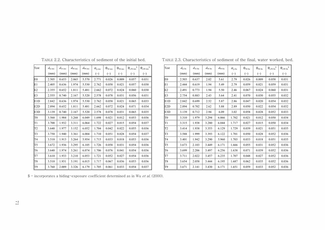
71

TABLE 2.2. Characteristics of sediment of the initial bed. TABLE 2.3. Characteristics of sediment of the final, water worked, bed.

Test dm inic d16 inic d50 inic d90 inic σg inic θ50 inic θ90 inic θc50 inic$ θc90 inic

$ Test dm fin d16 fin d50 fin d90 fin σg fin θ50 fin θ90 fin θc50 fin$ θc90 fin

$

(mm) (mm) (mm) (mm) (−) (−) (−) (−) (−) (mm) (mm) (mm) (mm) (−) (−) (−) (−) (−)

E0 2.505 0.653 2.065 5.570 2.771 0.026 0.009 0.057 0.031 E0 2.503 0.637 2.02 5.61 2.79 0.026 0.009 0.058 0.031

E1 2.405 0.636 1.974 5.530 2.762 0.058 0.021 0.057 0.030 E1 2.444 0.619 1.94 5.49 2.79 0.059 0.021 0.059 0.031

E2 2.355 0.652 1.811 5.481 2.662 0.072 0.024 0.060 0.030 E2 2.491 0.773 1.94 5.50 2.46 0.067 0.024 0.060 0.031

E3 2.555 0.740 2.167 5.520 2.578 0.078 0.031 0.056 0.031 E3 2.754 0.883 2.43 5.64 2.41 0.070 0.030 0.055 0.032

E1D 2.842 0.636 1.974 5.530 2.762 0.058 0.021 0.065 0.033 E1D 2.842 0.699 2.52 5.87 2.86 0.047 0.020 0.054 0.032

E2D 2.894 0.652 1.811 5.481 2.662 0.072 0.024 0.071 0.034 E2D 2.894 0.702 2.62 5.88 2.89 0.050 0.022 0.054 0.032

E3D 3.139 0.740 2.167 5.520 2.578 0.078 0.031 0.065 0.035 E3D 3.139 0.712 2.94 6.09 3.02 0.058 0.028 0.052 0.033

T0 3.560 1.984 3.268 6.049 1.698 0.021 0.012 0.053 0.036 T0 3.310 1.979 3.294 6.066 1.702 0.021 0.012 0.050 0.034

T1 3.700 1.932 3.311 6.064 1.722 0.027 0.015 0.054 0.037 T1 3.315 1.938 3.280 6.044 1.717 0.027 0.015 0.050 0.034

T2 3.640 1.977 3.152 6.052 1.704 0.042 0.022 0.055 0.036 T2 3.414 1.938 3.353 6.129 1.729 0.039 0.021 0.051 0.035

T3 3.750 1.940 3.361 6.004 1.710 0.051 0.028 0.054 0.037 T3 3.588 1.999 3.393 6.122 1.701 0.050 0.028 0.052 0.036

T4 3.510 1.913 3.264 5.954 1.715 0.033 0.018 0.053 0.036 T4 3.401 1.942 3.290 5.960 1.703 0.033 0.018 0.051 0.035

T5 3.672 1.936 3.295 6.105 1.726 0.058 0.031 0.054 0.036 T5 3.673 2.103 3.449 6.171 1.666 0.055 0.031 0.052 0.036

T6 3.640 1.974 3.261 6.074 1.706 0.076 0.041 0.054 0.036 T6 3.699 2.206 3.497 6.256 1.638 0.071 0.039 0.052 0.036

T7 3.610 1.933 3.210 6.053 1.721 0.052 0.027 0.054 0.036 T7 3.711 2.022 3.457 6.235 1.707 0.048 0.027 0.052 0.036

T8 3.510 1.931 3.191 6.015 1.717 0.067 0.036 0.053 0.036 T8 3.654 2.058 3.444 6.195 1.687 0.062 0.035 0.052 0.036

T9 3.760 2.009 3.326 6.179 1.705 0.061 0.033 0.054 0.037 T9 3.671 2.141 3.430 6.171 1.651 0.059 0.033 0.052 0.036

$ - incorporates a hiding-exposure coefficient determined as in Wu et al. (2000).

71

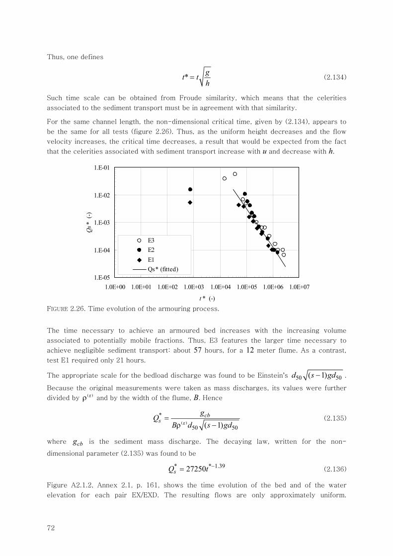
72

Thus, one defines

* gt th

= (2.134)

Such time scale can be obtained from Froude similarity, which means that the celerities

associated to the sediment transport must be in agreement with that similarity.

For the same channel length, the non-dimensional critical time, given by (2.134), appears to

be the same for all tests (figure 2.26). Thus, as the uniform height decreases and the flow

velocity increases, the critical time decreases, a result that would be expected from the fact

that the celerities associated with sediment transport increase with u and decrease with h.

1.E-05

1.E-04

1.E-03

1.E-02

1.E-01

1.0E+00 1.0E+01 1.0E+02 1.0E+03 1.0E+04 1.0E+05 1.0E+06 1.0E+07

t * (-)

Qs*

(-)

E3E2E1Qs* (fitted)

FIGURE 2.26. Time evolution of the armouring process.

The time necessary to achieve an armoured bed increases with the increasing volume

associated to potentially mobile fractions. Thus, E3 features the larger time necessary to

achieve negligible sediment transport: about 57 hours, for a 12 meter flume. As a contrast,

test E1 required only 21 hours.

The appropriate scale for the bedload discharge was found to be Einstein’s 50 50( 1)d s gd− .

Because the original measurements were taken as mass discharges, its values were further

divided by ( )gρ and by the width of the flume, B. Hence

( )

*

50 50( 1)g

cbs

gQ

B d s gd=

ρ − (2.135)

where cbg is the sediment mass discharge. The decaying law, written for the non-

dimensional parameter (2.135) was found to be

* * 1.3927250sQ t −= (2.136)

Figure A2.1.2, Annex 2.1, p. 161, shows the time evolution of the bed and of the water

elevation for each pair EX/EXD. The resulting flows are only approximately uniform.

73

However, at the location of the Laser optics, it is observable that the flow profiles are

comparable to those of the equilibrium flows. Any non-uniform flow effects are, thus,

disregarded.

As for tests of series T, only T6 was designed to have nearly all size fractions in the bedload;

only the very large clasts, about the size of d100 were to remain stable. Tests T8 and T9 show

great mobility but size fractions larger than the d80 should not be entrained. Tests T0, T1, T2

and T4 were designed so that only the very fine gravel would move. Tests T3, T5, T7 have

intermediate mobilities between T9 and T2.

The characteristic diameters of the final and of the initial beds of tests E and T are seen in

table 2.3 and compared in figure 2.27. It is evident that water worked bed are coarser than

the initial bed if the applied shear stress is high. Indeed, in the case of tests of series E, it E3

that shows the greater difference, consistent in the three characteristic grain diameters. In

series T, it is clear that the tests for which the applied shear stress is low (T0, θ50 = 0.021,

T1, θ50 = 0.027, T2, θ50 = 0.039 and T4, θ50 = 0.033) do not show appreciable differences in

the composition of the initial and final beds. It is the tests with higher shear stresses, notably

T6 (θ50 = 0.076) and T8 (θ50 = 0.071) that show the greater coarsening.

It can only be concluded that the process of entraining and deposiotion of sediment into the

bedload was initially a non-equilibrium one. In the process of attining equilibrium transport

conditions, a certain amount of volume of the finer fractions was buried and the surface

became coarser. This subject will be addressed again in §2.4.6, p. 133.

2.4 EXPERIMENTAL RESULTS AND DEVELOPMENT OF THE CLOSURE SUB-MODEL

2.4.1 Velocity profiles and turbulent characteristics

Boundary layer flows confined by smooth fixed walls provided the framework for the study of

the velocity profiles in turbulent open-channel flows. The work of Prandtl, 1930 (cf., e.g.,

White 1986, p. 299), provides a clear, if not totally undisputed (cf. Pope 2000, p. 367),

framework for the derivation of the velocity profiles. In a two-dimensional flow, uniform in

the longitudinal direction, open-channel flow with a fixed boundary, assuming that the

boundary layer is fully developed, i.e., that the turbulent boundary layer occupies the whole

of the flow depth, the equation of conservation of momentum in the along-stream direction

renders, if integrated with the appropriate boundary conditions (Townsend 1976, p. 131), the

following equation for the shear stress

( )( ) ( ) ( )dw w wyx yT u uv= μ − ρ (2.137)

where u u u= − and v v v= − are the velocity fluctuations in the longitudinal and normal

directions. The product of the shear rate and the fluid viscosity, ( )( )dwy uμ , represents the

viscous stresses and ( )w uv−ρ , named Reynolds stresses, stands for the turbulent stresses. It

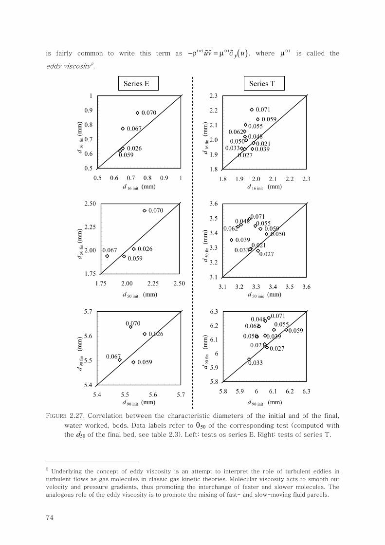
74

is fairly common to write this term as ( )( ) ( )w tyuv u−ρ = μ ∂ , where

( )tμ is called the

eddy viscosity5.

0.070

0.067

0.0590.026

0.5

0.6

0.7

0.8

0.9

1

0.5 0.6 0.7 0.8 0.9 1d 16 init (mm)

d16

fin

(mm

)

0.0710.059

0.0550.062

0.0480.050 0.021

0.0270.0390.033

1.8

1.9

2.0

2.1

2.2

2.3

1.8 1.9 2.0 2.1 2.2 2.3d 16 init (mm)

d16

fin

(mm

)

0.0670.059

0.026

0.070

1.75

2.00

2.25

2.50

1.75 2.00 2.25 2.50

d 50 init (mm)

d50

fin (

mm

)

0.0550.059

0.0500.039

0.0710.048

0.062

0.0210.0270.033

3.1

3.2

3.3

3.4

3.5

3.6

3.1 3.2 3.3 3.4 3.5 3.6d 50 inic (mm)

d50

fin

(mm

)

0.026

0.059

0.070

0.067

5.4

5.5

5.6

5.7

5.4 5.5 5.6 5.7d 90 init (mm)

d90

fin

(mm

)

0.0390.021 0.027

0.033

0.0550.0620.059

0.0710.048

0.050

5.8

5.9

6

6.1

6.2

6.3

5.8 5.9 6 6.1 6.2 6.3

d 90 init (mm)

d90

fin

(mm

)

FIGURE 2.27. Correlation between the characteristic diameters of the initial and of the final,

water worked, beds. Data labels refer to θ50 of the corresponding test (computed with

the d50 of the final bed, see table 2.3). Left: tests os series E. Right: tests of series T.

5 Underlying the concept of eddy viscosity is an attempt to interpret the role of turbulent eddies in

turbulent flows as gas molecules in classic gas kinetic theories. Molecular viscosity acts to smooth out

velocity and pressure gradients, thus promoting the interchange of faster and slower molecules. The

analogous role of the eddy viscosity is to promote the mixing of fast- and slow-moving fluid parcels.

Series E Series T

75

Reynolds stresses are, according to Prandtl, op. cit., adequately modelled with the help of the

concept of mixing length, , loosely defined as the size of the eddies that promote mixing of

fast- and slow-moving fluid across and along the flow. The usual definition is

( )( )22 d yuv u− ≡ . A combination of along-stream and normal equations of conservation of

momentum renders the triangular shear stress profile shown in figure 2.69,

( )( ) ( ) 2* 1w w

yxT u y h= ρ − . Inserting these two equations in (2.137) one obtains

( ) ( ) ( ) ( )( ) ( ) ( )2 2*d d d 1w w w

y y yu u u u y hρ + μ = ρ − (2.138)

The numerical solution of (2.138) determines the velocity profile over the flow depth.

Analytical expressions for the entire flow depth are not generally attainable. But it is easily

verified that equation (2.138) represents a multiple-scale problem. The mixing length is

necessarily very small at the vicinity of the boundary and, as a consequence, the first term of

the left-hand side of (2.138) vanishes. Hence, the solution of the equation (2.138) changes

considerably from the boundary region to the outer flow region.

The multiple-scale nature of the problem is associated to a specific flow subdivision. Near

the wall there is an inner layer where flow is much influenced by the existence of a solid

boundary where the velocity is zero; hence, in this layer, the flow undergoes appreciable

shear. The upper flow regions are much influenced by the free surface, in particular its

vertical displacements, commanded by extraneous actions like wind shear; following Nezu &

Nakagawa (1993), p. 19, this region will be termed the free surface layer. In between these

layers there is a transition region sometimes called the equilibrium layer or, simply, the

intermediate layer. This subdivision can be seen in figure 2.28.

It is pertinent to pay further attention to energetic arguments underlying this subdivision. For

instance, the concept of equilibrium layer is called forth because it is expected that

production and dissipation of turbulent kinetic energy are in equilibrium. In general, it can be

established an association between regions of production, dissipation and diffusion of

turbulent kinetic energy and flow layers. For a better understanding, the equation of

conservation of the turbulent kinetic energy is recalled. Using a combination of tensor and

Leibnitz notation, it can be written (cf., Townsend 1976, p. 124)

( ) ( ) ( )( )

( ) ( ) ( ) ( )

( ) ( ) ( )

( ) ( ) ( )

A B C12

FD E

w w w

j j j

w w w

j j k k

t x j x x

x j i i j j i x i x i x i

k u k k

u u u pu u u u u u

∂ ρ + ∂ ρ = ∂ μ ∂

− ∂ ρ + −ρ ∂ − μ ∂ ∂

(2.139)

where the turbulent kinetic energy is defined as

( )2 2 211 2 32k u u u= + + (2.140)

In the above equations, ju stands for the velocity fluctuations in the longitudinal (j = 1),

normal (j = 2) and transverse (j = 3) directions, p is the fluid pressure and the overbar stands

for time average.

76

On the left-hand side, term A stands for energy accumulation or, equivalently, local energy

variation. Term B stands for the convective transport of energy. The sum of these terms

constitutes the material variation of the turbulent kinetic energy. On the right-hand side, term

C represents molecular viscous diffusion. Term D is also a diffusion term; it represents

turbulent diffusion and is generally modelled as an analogy to the viscous diffusion, i.e.,

( ) ( )( )( ) ( )12

w t

j j jx j i i j x xu u u pu k∂ ρ + = ∂ μ ∂ where μ(t) is the eddy viscosity. Term E, the

product of the turbulent shear stresses and the shear rate, represents the production of

turbulent kinetic energy, while term F stands for “turbulent” dissipation. It should be

remembered that the dissipation is always of viscous nature. The epithet “turbulent” serves to

highlight the role of turbulence in the process, i.e., conveying energy from the larger eddies

to the smaller eddies, a process called cascading, so that the actual molecular dissipation can

act when the eddies are of sufficiently small size (cf. Kolmogorov 1962).

In a two-dimensional, steady, uniform (in the longitudinal direction) flow, the time material

derivative is zero and equation (2.139) becomes

( )( ) ( ) ( ) ( ) ( )

( )( ) ( )( ) ( )( )

( ) ( ) ( ) ( )

( ) ( ) ( )

2 2 2 212

2 2 20

w w w w

w w w

y y y y y y

y y y

k v u v w pv uv u v v

u v w

⎛ ⎞∂ μ ∂ − ∂ ρ + + − ∂ − ρ ∂ − ρ ∂⎜ ⎟⎝ ⎠

−μ ∂ − μ ∂ − μ ∂ =

Given that the flow is incompressible, that the fluid is homogeneous and that the mean normal

velocity is approximately zero6, i.e., that ( ) 0y v∂ ≈ , the equation above becomes

( ) ( )

( ) ( )( ) ( )( ) ( )( )

( )2 2 2 21

2C D1 D2

2 2 2

EF

0

wy y y

y y y y

pk v u v w v

uv u u v w

⎛ ⎞⎛ ⎞υ∂ − ∂ + + − ∂ +⎜ ⎟ ⎜ ⎟ρ⎝ ⎠ ⎝ ⎠

⎛ ⎞− ∂ − υ ∂ + ∂ + ∂ =⎜ ⎟

⎝ ⎠

(2.141)

where υ is the cinematic viscosity of the water. The time-avergaed velocity u will be herein

designated simply as u.

Restricting, for now, the analysis to flows with smooth boundaries, it is noted that viscous

diffusion is negligible at high Reynolds numbers, except at a small bounded region near the

fixed boundary. Thus, a more detailed flow subdivision must be undertaken. The region where

term C is not negligible is called the viscous sub-layer (figure 2.28). It is characterized by

important viscous stresses and negligible turbulent stresses. Direct viscous dissipation is, in

this region, a sink of kinetic energy of the mean flow. Associated to the direct dissipation of

mean kinetic energy, there is the diffusion of k away from the boundary. If term C is

negligible outside the viscous sub-layer; turbulent production, term E, is negligible inside it,

because so are the Reynolds stresses.

6 This result comes from the equation of conservation of mass, in the hypothesis that the longitudinal

pressure gradient is zero, i.e., that the flow is uniform in the longitudinal direction.

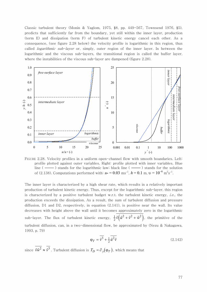
77

Classic turbulent theory (Monin & Yaglom, 1975, §8, pp. 449-567, Townsend 1976, §5),

predicts that sufficiently far from the boundary, yet still within the inner layer, production

(term E) and dissipation (term F) of turbulent kinetic energy cancel each other. As a

consequence, (see figure 2.28 below) the velocity profile is logarithmic in this region, thus

called logarithmic sub-layer or, simply, outer region of the inner layer. In between the

logarithmic and the viscous sub-layers, the transitional region is called the buffer layer,

where the instabilities of the viscous sub-layer are dampened (figure 2.28).

0.0

0.1

0.2

0.3

0.4

0.5

0.6

0.7

0.8

0.9

1.0

0 5 10 15 20 25u/u * (-)

y/h

(-)

free-surface layer

intermediate layer

inner layer logarithmic

buffer viscous 0

5

10

15

20

25

0.001 0.01 0.1 1 10 100 1000y + (-)

u+ (-

)

free-surface layerinterm

ediate layer inner layer

logarithmic

buffer

viscous

FIGURE 2.28. Velocity profiles in a uniform open-channel flow with smooth boundaries. Left:

profile plotted against outer variables. Right: profile plotted with inner variables. Blue

line ( ) stands for the logarithmic law; black line ( ) stands for the solution

of (2.138). Computations performed with: u* = 0.03 ms−1, h = 0.1 m, υ = 10−6 m2s−1.

The inner layer is characterized by a high shear rate, which results in a relatively important

production of turbulent kinetic energy. Thus, except for the logarithmic sub-layer, this region

is characterized by a positive turbulent budget w.r.t. the turbulent kinetic energy, i.e., the

production exceeds the dissipation. As a result, the sum of turbulent diffusion and pressure

diffusion, D1 and D2, respectively, in equation (2.141), is positive near the wall. Its value

decreases with height above the wall until it becomes approximately zero in the logarithmic

sub-layer. The flux of turbulent kinetic energy, ( )2 2 212 v u v w+ + , the primitive of the

turbulent diffusion, can, in a two-dimensional flow, be approximated by (Nezu & Nakagawa,

1993, p. 79)

3 21

2T v u vϕ = + (2.142)

since 2 3vw v≈ . Turbulent diffusion is ( )D y TT = ∂ ϕ , which means that

78

( ) ( ) dy

T T Dy T yυ

υδ

ϕ = ϕ δ + ∫ .

where δυ, the thickness of the viscous sub-layer, is a very small quantity. Hence, if the flux

is zero at the vicinity of the boundary, it is expected that the flux of turbulent kinetic energy

is directed upwards in the region where turbulent diffusion is positive. One is assuming that

total diffusion and pressure diffusion have the same signal, i.e., that pressure diffusion (D2)

does not change the signal of turbulent diffusion. This is known to be the case in most

boundary layer flows, where the role of particle diffusion (D2) is only residual.

The intermediate layer has, fundamentally, the same characteristics of the logarithmic

sublayer. In particular, the production and the dissipation of turbulent kinetic energy cancel

each other and the velocity profile is logarithmic.

In the free-surface layer, dissipation is dominant, not because its absolute value is large, but

because production is vanishing. As a result, turbulent diffusion must act to supply kinetic

energy from the inner layer to this layer, through the intermediate layer. These

considerations about the turbulent kinetic energy budget back the multiple scale argument

stated before.

An effective way to state the multiple scale argument, for the purpose of the derivation of the

straightforward expressions for velocity profiles, requires the dimensional analysis of the

vertical velocity distribution, through the analysis of the shear rate. It follows from equation

(2.139) that the vertical velocity distribution obeys the dimensional relation

( ) ( )( ) ( )*d , , , ,w w

y u f y h u= μ ρ (2.143)

where the friction velocity appears in substitution of the bed shear stress. Applying Vaschy-

Buckingam’s theorem the above equation becomes

( ) ( )( )

( )

*1 1

* **

d d, ,

w

w

y yy u y u yuh hu y u yy u− −

⎛ ⎞ ⎛ ⎞ρ= Π ⇔ = Π⎜ ⎟ ⎜ ⎟⎜ ⎟ υμ ⎝ ⎠⎝ ⎠

(2.144)

Clearly, equation (2.144) states that there are two length scales for the velocity profile, h, an

outer variable, and u*/υ, an inner scale. In general, all scales that involve the viscosity or the

bed shear stress are called inner scales because viscosity and shear are most important near

the boundary. If complete similarity is postulated, taking the appropriate limits to the non-

dimensional parameters may render the desired expressions for the velocity profile (cf.

Barenblatt 1996, p. 158, 270). Thus, in the inner region yet far from the boundary, 1y h ,

thus 1h y , but * 1yu υ . Under complete similarity ( ), cteΠ ∞ ∞ = and (2.144) becomes

( )

( )( )0

0

* * *

d ( ) ( ) 1 ( )d lny

y

y

y u u y u y u ycte cte cte y Au u u

η=

η=

−= ⇔ = η ⇔ = −

η∫

This equation is generally written in such way that the height above the bed is scaled by the

inner length. Also, the multiplying constant, which bears the name of the precursor of this

technique, the Hungarian engineer von Kármán, as been seen to be 1 10.4cte κ≡ . Introducing

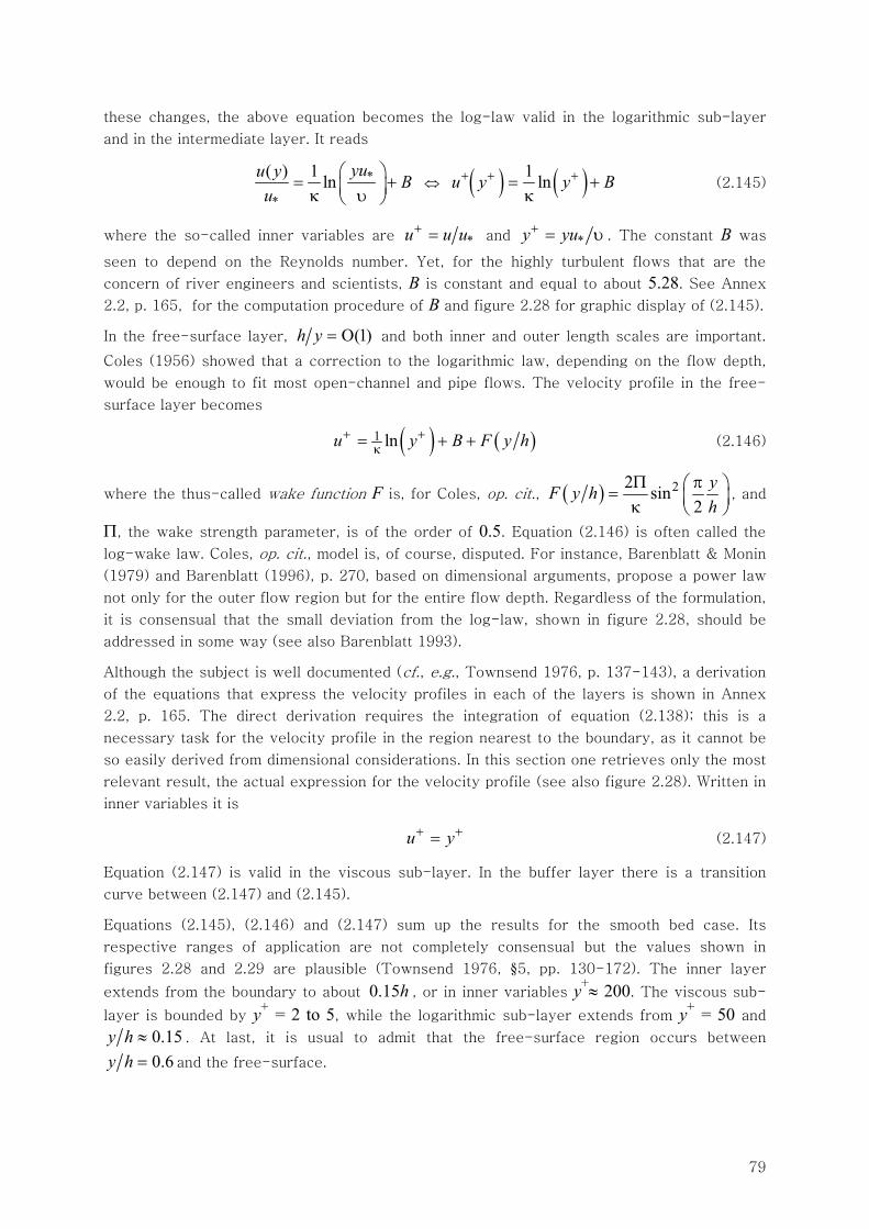
79

these changes, the above equation becomes the log-law valid in the logarithmic sub-layer

and in the intermediate layer. It reads

*

*

( ) 1 lnyuu y B

u⎛ ⎞= +⎜ ⎟κ υ⎝ ⎠

⇔ ( ) ( )1 lnu y y B+ + += +κ

(2.145)

where the so-called inner variables are *u u u+ = and *y yu+ = υ . The constant B was

seen to depend on the Reynolds number. Yet, for the highly turbulent flows that are the

concern of river engineers and scientists, B is constant and equal to about 5.28. See Annex

2.2, p. 165, for the computation procedure of B and figure 2.28 for graphic display of (2.145).

In the free-surface layer, O(1)h y = and both inner and outer length scales are important.

Coles (1956) showed that a correction to the logarithmic law, depending on the flow depth,

would be enough to fit most open-channel and pipe flows. The velocity profile in the free-

surface layer becomes

( ) ( )1 lnu y B F y h+ +κ= + + (2.146)

where the thus-called wake function F is, for Coles, op. cit., ( ) 22 sin2

yF y hh

Π π⎛ ⎞= ⎜ ⎟κ ⎝ ⎠, and

Π, the wake strength parameter, is of the order of 0.5. Equation (2.146) is often called the

log-wake law. Coles, op. cit., model is, of course, disputed. For instance, Barenblatt & Monin

(1979) and Barenblatt (1996), p. 270, based on dimensional arguments, propose a power law

not only for the outer flow region but for the entire flow depth. Regardless of the formulation,

it is consensual that the small deviation from the log-law, shown in figure 2.28, should be

addressed in some way (see also Barenblatt 1993).

Although the subject is well documented (cf., e.g., Townsend 1976, p. 137-143), a derivation

of the equations that express the velocity profiles in each of the layers is shown in Annex

2.2, p. 165. The direct derivation requires the integration of equation (2.138); this is a

necessary task for the velocity profile in the region nearest to the boundary, as it cannot be

so easily derived from dimensional considerations. In this section one retrieves only the most

relevant result, the actual expression for the velocity profile (see also figure 2.28). Written in

inner variables it is

u y+ += (2.147)

Equation (2.147) is valid in the viscous sub-layer. In the buffer layer there is a transition

curve between (2.147) and (2.145).

Equations (2.145), (2.146) and (2.147) sum up the results for the smooth bed case. Its

respective ranges of application are not completely consensual but the values shown in

figures 2.28 and 2.29 are plausible (Townsend 1976, §5, pp. 130-172). The inner layer

extends from the boundary to about 0.15h , or in inner variables y+≈ 200. The viscous sub-

layer is bounded by y+ = 2 to 5, while the logarithmic sub-layer extends from y+ = 50 and

0.15y h ≈ . At last, it is usual to admit that the free-surface region occurs between

0.6y h = and the free-surface.

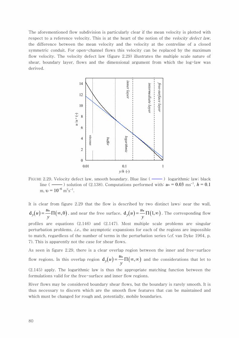
80

The aforementioned flow subdivision is particularly clear if the mean velocity is plotted with

respect to a reference velocity. This is at the heart of the notion of the velocity defect law,

the difference between the mean velocity and the velocity at the centreline of a closed

symmetric conduit. For open-channel flows this velocity can be replaced by the maximum

flow velocity. The velocity defect law (figure 2.29) illustrates the multiple scale nature of

shear, boundary layer, flows and the dimensional argument from which the log-law was

derived.

0

2

4

6

8

10

12

14

0.01 0.1 1y/h (-)

u/u

* (-)

free-surface layer

intermediate layer

inner layer logarithm

ic

bu ffer

viscous

FIGURE 2.29. Velocity defect law, smooth boundary. Blue line ( ) logarithmic law; black

line ( ) solution of (2.138). Computations performed with: u* = 0.03 ms−1, h = 0.1

m, υ = 10−6 m2s−1.

It is clear from figure 2.29 that the flow is described by two distinct laws: near the wall,

( ) ( )*d ,0yuuy

= Π ∞ , and near the free surface, ( ) ( )*d 1,yuuy

= Π ∞ . The corresponding flow

profiles are equations (2.146) and (2.147). Most multiple scale problems are singular

perturbation problems, i.e., the asymptotic expansions for each of the regions are impossible

to match, regardless of the number of terms in the perturbation series (cf. van Dyke 1964, p.

7). This is apparently not the case for shear flows.

As seen in figure 2.29, there is a clear overlap region between the inner and free-surface

flow regions. In this overlap region ( ) ( )*d ,yu

uy

= Π ∞ ∞ and the considerations that let to

(2.145) apply. The logarithmic law is thus the appropriate matching function between the

formulations valid for the free-surface and inner flow regions.

River flows may be considered boundary shear flows, but the boundary is rarely smooth. It is

thus necessary to discern which are the smooth flow features that can be maintained and

which must be changed for rough and, potentially, mobile boundaries.

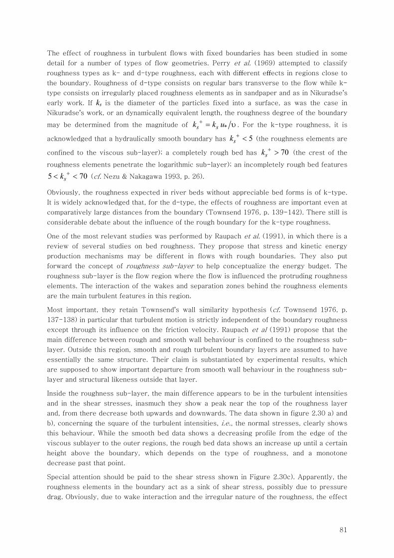
81

The effect of roughness in turbulent flows with fixed boundaries has been studied in some

detail for a number of types of flow geometries. Perry et al. (1969) attempted to classify

roughness types as k- and d-type roughness, each with different effects in regions close to

the boundary. Roughness of d-type consists on regular bars transverse to the flow while k-

type consists on irregularly placed roughness elements as in sandpaper and as in Nikuradse’s

early work. If ks is the diameter of the particles fixed into a surface, as was the case in

Nikuradse’s work, or an dynamically equivalent length, the roughness degree of the boundary

may be determined from the magnitude of *s sk k u+ = υ . For the k-type roughness, it is

acknowledged that a hydraulically smooth boundary has 5sk + < (the roughness elements are

confined to the viscous sub-layer); a completely rough bed has 70sk + > (the crest of the

roughness elements penetrate the logarithmic sub-layer); an incompletely rough bed features

5 70sk +< < (cf. Nezu & Nakagawa 1993, p. 26).

Obviously, the roughness expected in river beds without appreciable bed forms is of k-type.

It is widely acknowledged that, for the d-type, the effects of roughness are important even at

comparatively large distances from the boundary (Townsend 1976, p. 139-142). There still is

considerable debate about the influence of the rough boundary for the k-type roughness.

One of the most relevant studies was performed by Raupach et al. (1991), in which there is a

review of several studies on bed roughness. They propose that stress and kinetic energy

production mechanisms may be different in flows with rough boundaries. They also put

forward the concept of roughness sub-layer to help conceptualize the energy budget. The

roughness sub-layer is the flow region where the flow is influenced the protruding roughness

elements. The interaction of the wakes and separation zones behind the roughness elements

are the main turbulent features in this region.

Most important, they retain Townsend’s wall similarity hypothesis (cf. Townsend 1976, p.

137-138) in particular that turbulent motion is strictly independent of the boundary roughness

except through its influence on the friction velocity. Raupach et al (1991) propose that the

main difference between rough and smooth wall behaviour is confined to the roughness sub-

layer. Outside this region, smooth and rough turbulent boundary layers are assumed to have

essentially the same structure. Their claim is substantiated by experimental results, which

are supposed to show important departure from smooth wall behaviour in the roughness sub-

layer and structural likeness outside that layer.

Inside the roughness sub-layer, the main difference appears to be in the turbulent intensities

and in the shear stresses, inasmuch they show a peak near the top of the roughness layer

and, from there decrease both upwards and downwards. The data shown in figure 2.30 a) and

b), concerning the square of the turbulent intensities, i.e., the normal stresses, clearly shows

this behaviour. While the smooth bed data shows a decreasing profile from the edge of the

viscous sublayer to the outer regions, the rough bed data shows an increase up until a certain

height above the boundary, which depends on the type of roughness, and a monotone

decrease past that point.

Special attention should be paid to the shear stress shown in Figure 2.30c). Apparently, the

roughness elements in the boundary act as a sink of shear stress, possibly due to pressure

drag. Obviously, due to wake interaction and the irregular nature of the roughness, the effect

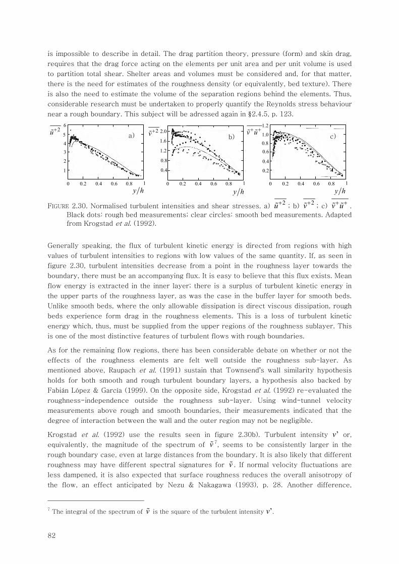
82

is impossible to describe in detail. The drag partition theory, pressure (form) and skin drag,

requires that the drag force acting on the elements per unit area and per unit volume is used

to partition total shear. Shelter areas and volumes must be considered and, for that matter,

there is the need for estimates of the roughness density (or equivalently, bed texture). There

is also the need to estimate the volume of the separation regions behind the elements. Thus,

considerable research must be undertaken to properly quantify the Reynolds stress behaviour

near a rough boundary. This subject will be adressed again in §2.4.5, p. 123.

FIGURE 2.30. Normalised turbulent intensities and shear stresses. a) 2u+

; b) 2v+

; c) v u+ +.

Black dots: rough bed measurements; clear circles: smooth bed measurements. Adapted

from Krogstad et al. (1992).

Generally speaking, the flux of turbulent kinetic energy is directed from regions with high

values of turbulent intensities to regions with low values of the same quantity. If, as seen in

figure 2.30, turbulent intensities decrease from a point in the roughness layer towards the

boundary, there must be an accompanying flux. It is easy to believe that this flux exists. Mean

flow energy is extracted in the inner layer; there is a surplus of turbulent kinetic energy in

the upper parts of the roughness layer, as was the case in the buffer layer for smooth beds.

Unlike smooth beds, where the only allowable dissipation is direct viscous dissipation, rough

beds experience form drag in the roughness elements. This is a loss of turbulent kinetic

energy which, thus, must be supplied from the upper regions of the roughness sublayer. This

is one of the most distinctive features of turbulent flows with rough boundaries.

As for the remaining flow regions, there has been considerable debate on whether or not the

effects of the roughness elements are felt well outside the roughness sub-layer. As

mentioned above, Raupach et al. (1991) sustain that Townsend’s wall similarity hypothesis

holds for both smooth and rough turbulent boundary layers, a hypothesis also backed by

Fabián López & García (1999). On the opposite side, Krogstad et al. (1992) re-evaluated the

roughness-independence outside the roughness sub-layer. Using wind-tunnel velocity

measurements above rough and smooth boundaries, their measurements indicated that the

degree of interaction between the wall and the outer region may not be negligible.

Krogstad et al. (1992) use the results seen in figure 2.30b). Turbulent intensity v’ or,

equivalently, the magnitude of the spectrum of v 7, seems to be consistently larger in the

rough boundary case, even at large distances from the boundary. It is also likely that different

roughness may have different spectral signatures for v . If normal velocity fluctuations are

less dampened, it is also expected that surface roughness reduces the overall anisotropy of

the flow, an effect anticipated by Nezu & Nakagawa (1993), p. 28. Another difference,

7 The integral of the spectrum of v is the square of the turbulent intensity v’.

0.6

0.2

0 0.2 0.4 0.6 0.8 1

0.4

0.8

1.0

1.2

c)

0.4

0.8

0 0.2 0.4 0.6 0.8 1

1.2

1.6

2.0b)

1

0 0.2 0.4 0.6 0.8 1

2

3

4

5

6

a)

y h y h y h

2u+ 2v+ v u+ +

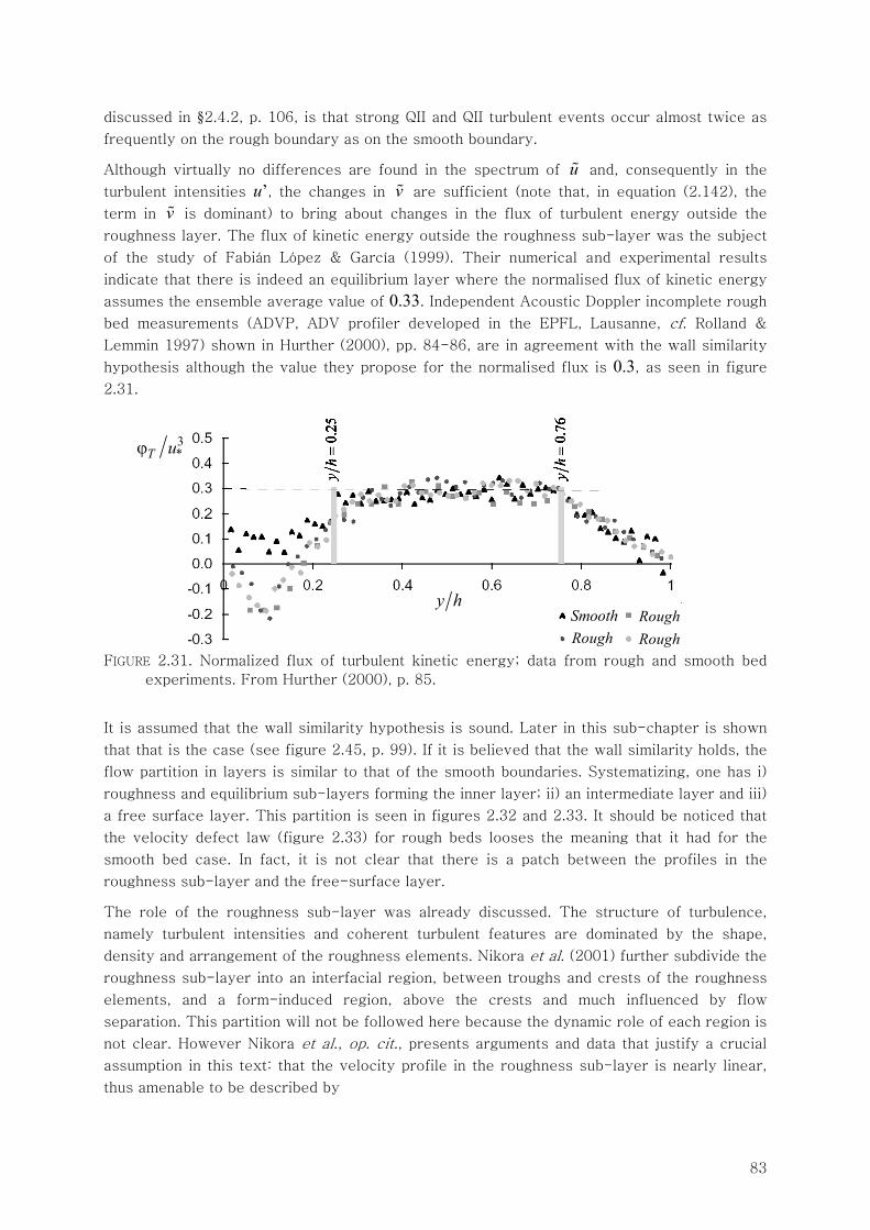
83

discussed in §2.4.2, p. 106, is that strong QII and QII turbulent events occur almost twice as

frequently on the rough boundary as on the smooth boundary.

Although virtually no differences are found in the spectrum of u and, consequently in the

turbulent intensities u’, the changes in v are sufficient (note that, in equation (2.142), the

term in v is dominant) to bring about changes in the flux of turbulent energy outside the

roughness layer. The flux of kinetic energy outside the roughness sub-layer was the subject

of the study of Fabián López & García (1999). Their numerical and experimental results

indicate that there is indeed an equilibrium layer where the normalised flux of kinetic energy

assumes the ensemble average value of 0.33. Independent Acoustic Doppler incomplete rough

bed measurements (ADVP, ADV profiler developed in the EPFL, Lausanne, cf. Rolland &

Lemmin 1997) shown in Hurther (2000), pp. 84-86, are in agreement with the wall similarity

hypothesis although the value they propose for the normalised flux is 0.3, as seen in figure

2.31.

FIGURE 2.31. Normalized flux of turbulent kinetic energy; data from rough and smooth bed

experiments. From Hurther (2000), p. 85.

It is assumed that the wall similarity hypothesis is sound. Later in this sub-chapter is shown

that that is the case (see figure 2.45, p. 99). If it is believed that the wall similarity holds, the

flow partition in layers is similar to that of the smooth boundaries. Systematizing, one has i)

roughness and equilibrium sub-layers forming the inner layer; ii) an intermediate layer and iii)

a free surface layer. This partition is seen in figures 2.32 and 2.33. It should be noticed that

the velocity defect law (figure 2.33) for rough beds looses the meaning that it had for the

smooth bed case. In fact, it is not clear that there is a patch between the profiles in the

roughness sub-layer and the free-surface layer.

The role of the roughness sub-layer was already discussed. The structure of turbulence,

namely turbulent intensities and coherent turbulent features are dominated by the shape,

density and arrangement of the roughness elements. Nikora et al. (2001) further subdivide the

roughness sub-layer into an interfacial region, between troughs and crests of the roughness

elements, and a form-induced region, above the crests and much influenced by flow

separation. This partition will not be followed here because the dynamic role of each region is

not clear. However Nikora et al., op. cit., presents arguments and data that justify a crucial

assumption in this text: that the velocity profile in the roughness sub-layer is nearly linear,

thus amenable to be described by

RoughRoughRough

Smooth

3*T uϕ

y h

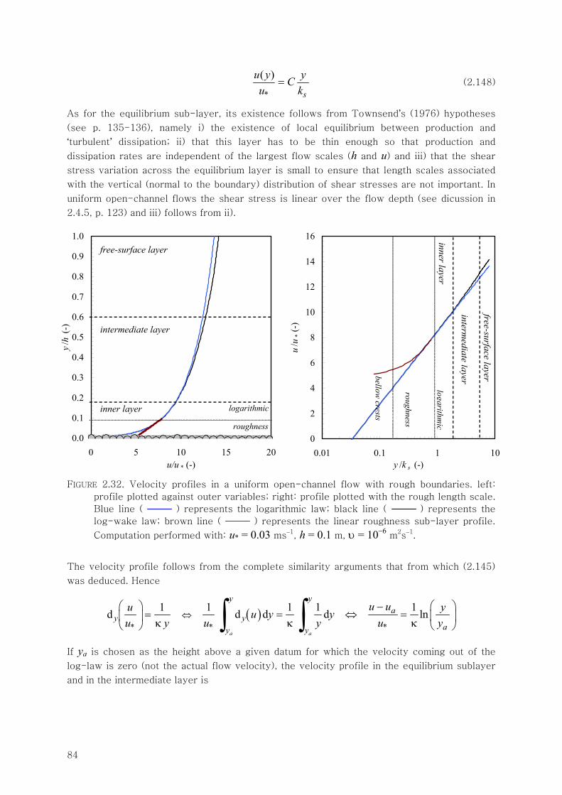
84

*

( )

s

u y yCu k

= (2.148)

As for the equilibrium sub-layer, its existence follows from Townsend’s (1976) hypotheses

(see p. 135-136), namely i) the existence of local equilibrium between production and

‘turbulent’ dissipation; ii) that this layer has to be thin enough so that production and

dissipation rates are independent of the largest flow scales (h and u) and iii) that the shear

stress variation across the equilibrium layer is small to ensure that length scales associated

with the vertical (normal to the boundary) distribution of shear stresses are not important. In

uniform open-channel flows the shear stress is linear over the flow depth (see dicussion in

2.4.5, p. 123) and iii) follows from ii).

0.0

0.1

0.2

0.3

0.4

0.5

0.6

0.7

0.8

0.9

1.0

0 5 10 15 20u/u * (-)

y/h

(-)

free-surface layer

intermediate layer

inner layer logarithmic

roughness0

2

4

6

8

10

12

14

16

0.01 0.1 1 10y /k s (-)

u/u

* (-)

free-surface layer

intermediate layer

inner layerlogarithm

ic

roughness

bellow crests

FIGURE 2.32. Velocity profiles in a uniform open-channel flow with rough boundaries. left:

profile plotted against outer variables; right: profile plotted with the rough length scale.

Blue line ( ) represents the logarithmic law; black line ( ) represents the

log-wake law; brown line ( ) represents the linear roughness sub-layer profile.

Computation performed with: u* = 0.03 ms−1, h = 0.1 m, υ = 10−6 m2s−1.

The velocity profile follows from the complete similarity arguments that from which (2.145)

was deduced. Hence

*

1d yuu y

⎛ ⎞=⎜ ⎟ κ⎝ ⎠

⇔ ( )* *

1 1 1 1d d d lna a

y ya

yay y

u u yu y yu y u y

⎛ ⎞−= ⇔ = ⎜ ⎟κ κ ⎝ ⎠∫ ∫

If ya is chosen as the height above a given datum for which the velocity coming out of the

log-law is zero (not the actual flow velocity), the velocity profile in the equilibrium sublayer

and in the intermediate layer is

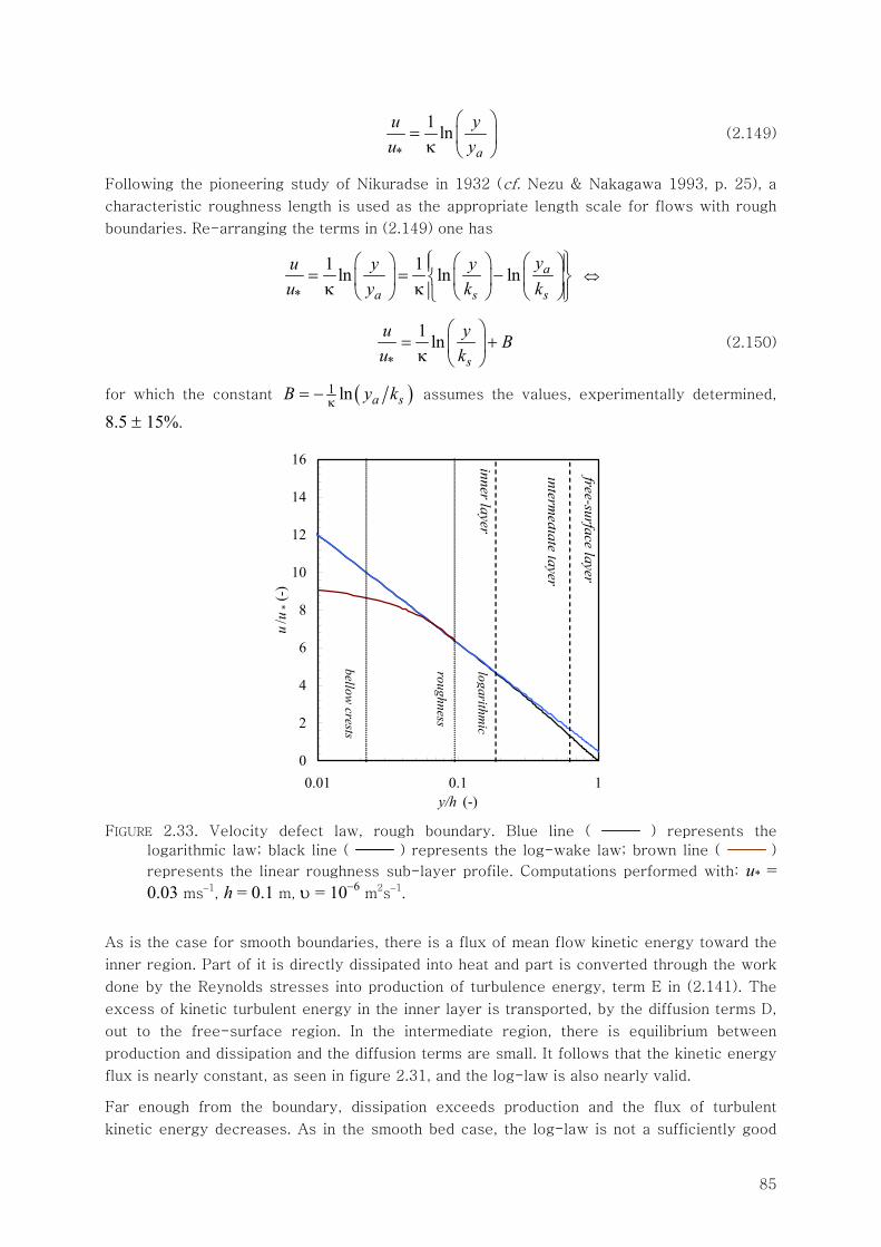
85

*

1 lna

u yu y

⎛ ⎞= ⎜ ⎟κ ⎝ ⎠

(2.149)

Following the pioneering study of Nikuradse in 1932 (cf. Nezu & Nakagawa 1993, p. 25), a

characteristic roughness length is used as the appropriate length scale for flows with rough

boundaries. Re-arranging the terms in (2.149) one has

*

1 1ln ln ln a

a s s

yu y yu y k k

⎧ ⎫⎛ ⎞ ⎛ ⎞ ⎛ ⎞⎪ ⎪= = −⎨ ⎬⎜ ⎟ ⎜ ⎟ ⎜ ⎟κ κ ⎪ ⎪⎝ ⎠ ⎝ ⎠ ⎝ ⎠⎩ ⎭ ⇔

*

1 lns

u y Bu k

⎛ ⎞= +⎜ ⎟κ ⎝ ⎠

(2.150)

for which the constant ( )1 ln a sB y kκ= − assumes the values, experimentally determined,

8.5 ± 15%.

0

2

4

6

8

10

12

14

16

0.01 0.1 1y/h (-)

u/u

* (-)

free-surface layer

intermediate layer

inner layerlogarithm

ic

roughness

bellow crests

FIGURE 2.33. Velocity defect law, rough boundary. Blue line ( ) represents the

logarithmic law; black line ( ) represents the log-wake law; brown line ( )

represents the linear roughness sub-layer profile. Computations performed with: u* = 0.03 ms−1, h = 0.1 m, υ = 10−6

m2s−1.

As is the case for smooth boundaries, there is a flux of mean flow kinetic energy toward the

inner region. Part of it is directly dissipated into heat and part is converted through the work

done by the Reynolds stresses into production of turbulence energy, term E in (2.141). The

excess of kinetic turbulent energy in the inner layer is transported, by the diffusion terms D,

out to the free-surface region. In the intermediate region, there is equilibrium between

production and dissipation and the diffusion terms are small. It follows that the kinetic energy

flux is nearly constant, as seen in figure 2.31, and the log-law is also nearly valid.

Far enough from the boundary, dissipation exceeds production and the flux of turbulent

kinetic energy decreases. As in the smooth bed case, the log-law is not a sufficiently good

86

description of the velocity profile and a correction, such as a wake law, should be considered.

Thus, the corresponding velocity profile may be

2

*

1 2ln sin2s

u y yBu k h

⎛ ⎞ Π π⎛ ⎞= + +⎜ ⎟ ⎜ ⎟κ κ ⎝ ⎠⎝ ⎠ (2.151)

Three main problems arise in the characterization of the velocity profiles: i) the location of

the datum; ii) the elevation of the log-law zero, ya; iii) the definition of the roughness scale ks.

In addition, there is also the problem of fitting Coles strength parameter, Π. The von Kármán

constant, κ, has been widely acknowledged to be approximately 0.4 for two-dimensional

open-channel and pipe flows. As for the constant B, it is fully determined by ya and ks.

Smart (1999) explicitly addressed the problem of determining the elevation of the log-law

zero, ya, and the location of the datum, y = 0 plane. He revises classic theories, namely

Nikuradse’s relation 30s ak y= . For Nikuradse the location of the y = 0 plane was

unambiguous; it was the surface on which its roughness elements were glued on. In a river

bed the plane y = 0 is more difficult to determine. Following Einstein’s early works (cf. Smart,

op. cit.), most researchers define the datum as the plane that is located δa below the elevation

of the crests of the roughness elements. This definition is not completely unambiguous if the

rough elements are non-homogeneous. Smart also recalls that this displacement distance has

been reported to be 0.2a skδ = or 3.85a ayδ = (for the atmospheric boundary layer). One

other way to define ya was fostered by van Rijn (1984), proposing ya = δυ + 0.03ks. It should

not be forgotten that Townsend (1976), p. 325, believes that ya is about one tenth of the

height of the roughness elements, which is may be expressed as ya = 0.1d90.

Smarts’, op. cit., own data show that, for ks = 10d90, the value of ks for which he achieved best

fits, δa = 1.1ya – 0.001 and ya = 0.07(u*/u*c)2, where u*c may be computed from Shields

critical bed shear stress. Given the uncertainty in defining the plane of the crests of the

roughness elements, the critical parameter for defining the datum, it is reasonable to ask, as

Smart, op. cit., did, if these best fits are not an attempt to force a logarithmic behaviour onto

the data. This care is especially stringent in the roughness layer.

Given the difficulty is defining the plane of the crests, a different conceptual route is followed

in this work. The following points configure the essential for the definition of the velocity

profiles presented in this work. The values of ks, ya, δa, B and Π are shown in table 2.4 for

each of the tests identified in table 2.1.

1) Bed profiles are taken by a point gage or, preferentially, by the high resolution electronic

profiler. Figure 2.34 shows an example from test E3D (see table 2.1) in which the step size of

the bed profiler was 2.5 mm. From this data, the distribution function of the bed area above

the lowest trough is calculated (see Parker et al. 2000). For each elevation, this function

assigns a percentage of the area of the cross-section of the longitudinal bed profile below

that elevation: if y < ylowest trough then Fb(y) = 0; if y < ylowest trough and y < yhigher crest then 0 < Fb(y) < 1; if y > yhigher crest then Fb(y) = 1. For this example, the distribution function is shown

in figure 2.35. The datum, y = 0, is defined as the elevation that corresponds to the percentile

15 of the bed area. The datum, i.e., the bed elevation is marked as a dotted line in figure 2.34.

2a) If the flow is below threshold for movement or armored or if the transport rates are low,

δa is the mean crest height above the bed elevation. It is computed as the difference between

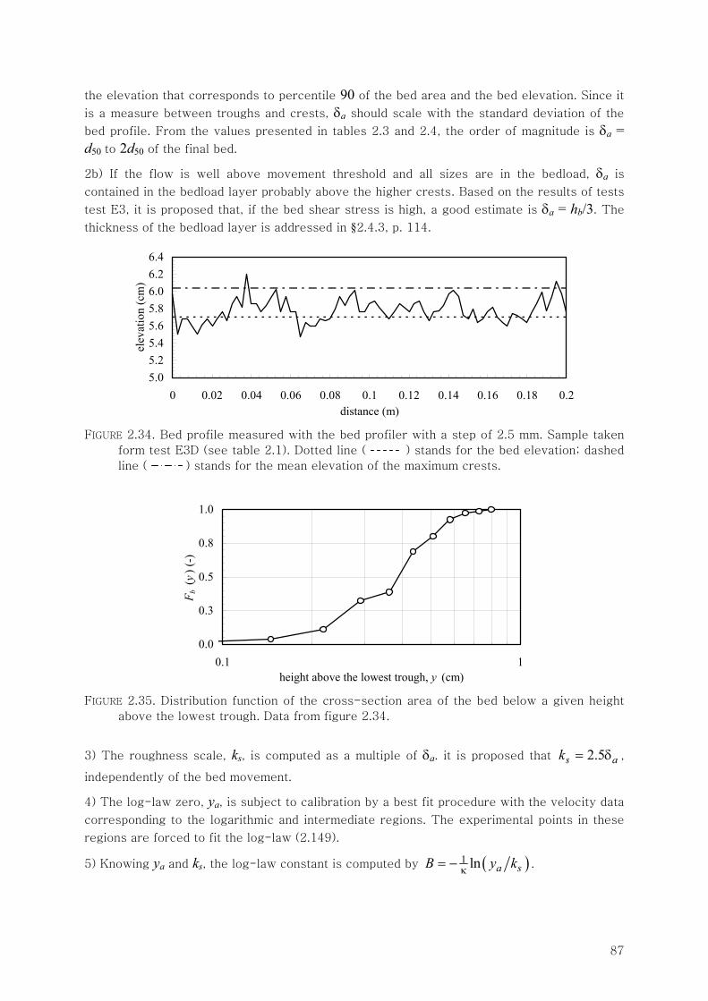
87

the elevation that corresponds to percentile 90 of the bed area and the bed elevation. Since it

is a measure between troughs and crests, δa should scale with the standard deviation of the

bed profile. From the values presented in tables 2.3 and 2.4, the order of magnitude is δa = d50 to 2d50 of the final bed.

2b) If the flow is well above movement threshold and all sizes are in the bedload, δa is

contained in the bedload layer probably above the higher crests. Based on the results of tests

test E3, it is proposed that, if the bed shear stress is high, a good estimate is δa = hb/3. The

thickness of the bedload layer is addressed in §2.4.3, p. 114.

5.05.25.45.65.86.06.26.4

0 0.02 0.04 0.06 0.08 0.1 0.12 0.14 0.16 0.18 0.2distance (m)

elev

atio

n (c

m)

FIGURE 2.34. Bed profile measured with the bed profiler with a step of 2.5 mm. Sample taken

form test E3D (see table 2.1). Dotted line ( ) stands for the bed elevation; dashed

line ( ) stands for the mean elevation of the maximum crests.

0.0

0.3

0.5

0.8

1.0

0.1 1height above the lowest trough, y (cm)

F b (y

) (-)

FIGURE 2.35. Distribution function of the cross-section area of the bed below a given height

above the lowest trough. Data from figure 2.34.

3) The roughness scale, ks, is computed as a multiple of δa. it is proposed that 2.5s ak = δ ,

independently of the bed movement.

4) The log-law zero, ya, is subject to calibration by a best fit procedure with the velocity data

corresponding to the logarithmic and intermediate regions. The experimental points in these

regions are forced to fit the log-law (2.149).

5) Knowing ya and ks, the log-law constant is computed by ( )1 ln a sB y kκ= − .

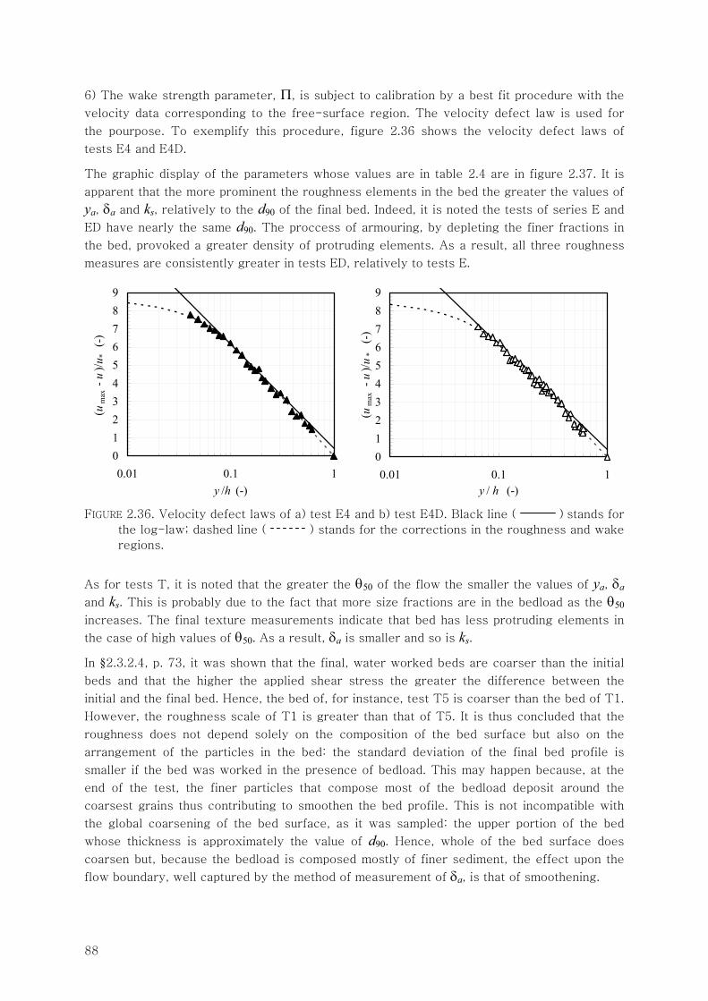
88

6) The wake strength parameter, Π, is subject to calibration by a best fit procedure with the

velocity data corresponding to the free-surface region. The velocity defect law is used for

the pourpose. To exemplify this procedure, figure 2.36 shows the velocity defect laws of

tests E4 and E4D.

The graphic display of the parameters whose values are in table 2.4 are in figure 2.37. It is

apparent that the more prominent the roughness elements in the bed the greater the values of

ya, δa and ks, relatively to the d90 of the final bed. Indeed, it is noted the tests of series E and

ED have nearly the same d90. The proccess of armouring, by depleting the finer fractions in

the bed, provoked a greater density of protruding elements. As a result, all three roughness

measures are consistently greater in tests ED, relatively to tests E.

0123456789

0.01 0.1 1y /h (-)

(um

ax -

u)/u

* (-

)

0123456789

0.01 0.1 1y / h (-)

(um

ax -

u)/u

* (-

)

FIGURE 2.36. Velocity defect laws of a) test E4 and b) test E4D. Black line ( ) stands for

the log-law; dashed line ( ) stands for the corrections in the roughness and wake

regions.

As for tests T, it is noted that the greater the θ50 of the flow the smaller the values of ya, δa

and ks. This is probably due to the fact that more size fractions are in the bedload as the θ50

increases. The final texture measurements indicate that bed has less protruding elements in

the case of high values of θ50. As a result, δa is smaller and so is ks.

In §2.3.2.4, p. 73, it was shown that the final, water worked beds are coarser than the initial

beds and that the higher the applied shear stress the greater the difference between the

initial and the final bed. Hence, the bed of, for instance, test T5 is coarser than the bed of T1.

However, the roughness scale of T1 is greater than that of T5. It is thus concluded that the

roughness does not depend solely on the composition of the bed surface but also on the

arrangement of the particles in the bed: the standard deviation of the final bed profile is

smaller if the bed was worked in the presence of bedload. This may happen because, at the

end of the test, the finer particles that compose most of the bedload deposit around the

coarsest grains thus contributing to smoothen the bed profile. This is not incompatible with

the global coarsening of the bed surface, as it was sampled: the upper portion of the bed

whose thickness is approximately the value of d90. Hence, whole of the bed surface does

coarsen but, because the bedload is composed mostly of finer sediment, the effect upon the

flow boundary, well captured by the method of measurement of δa, is that of smoothening.

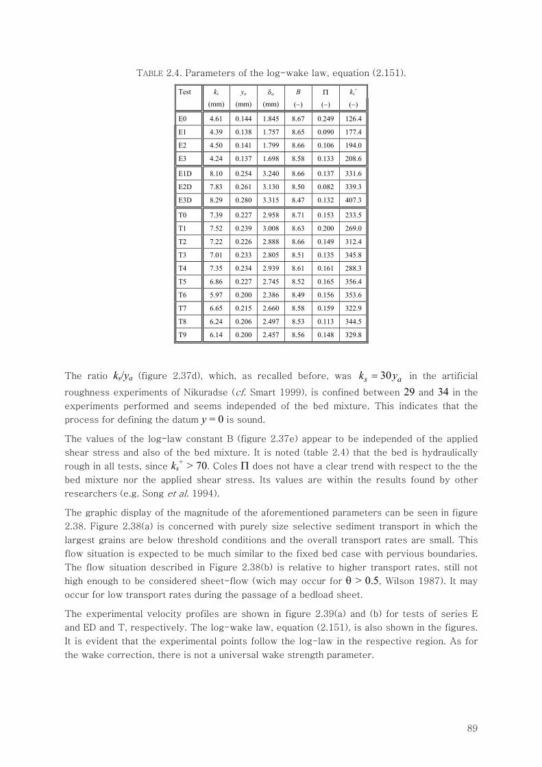
89

TABLE 2.4. Parameters of the log-wake law, equation (2.151).

Test ks ya δa B Π ks+

(mm) (mm) (mm) (−) (−) (−)

E0 4.61 0.144 1.845 8.67 0.249 126.4

E1 4.39 0.138 1.757 8.65 0.090 177.4

E2 4.50 0.141 1.799 8.66 0.106 194.0

E3 4.24 0.137 1.698 8.58 0.133 208.6

E1D 8.10 0.254 3.240 8.66 0.137 331.6

E2D 7.83 0.261 3.130 8.50 0.082 339.3

E3D 8.29 0.280 3.315 8.47 0.132 407.3

T0 7.39 0.227 2.958 8.71 0.153 233.5

T1 7.52 0.239 3.008 8.63 0.200 269.0

T2 7.22 0.226 2.888 8.66 0.149 312.4

T3 7.01 0.233 2.805 8.51 0.135 345.8

T4 7.35 0.234 2.939 8.61 0.161 288.3

T5 6.86 0.227 2.745 8.52 0.165 356.4

T6 5.97 0.200 2.386 8.49 0.156 353.6

T7 6.65 0.215 2.660 8.58 0.159 322.9

T8 6.24 0.206 2.497 8.53 0.113 344.5

T9 6.14 0.200 2.457 8.56 0.148 329.8

The ratio ks/ya (figure 2.37d), which, as recalled before, was 30s ak y= in the artificial

roughness experiments of Nikuradse (cf. Smart 1999), is confined between 29 and 34 in the

experiments performed and seems independed of the bed mixture. This indicates that the

process for defining the datum y = 0 is sound.

The values of the log-law constant B (figure 2.37e) appear to be independed of the applied

shear stress and also of the bed mixture. It is noted (table 2.4) that the bed is hydraulically

rough in all tests, since ks+ > 70. Coles Π does not have a clear trend with respect to the the

bed mixture nor the applied shear stress. Its values are within the results found by other

researchers (e.g. Song et al. 1994).

The graphic display of the magnitude of the aforementioned parameters can be seen in figure

2.38. Figure 2.38(a) is concerned with purely size selective sediment transport in which the

largest grains are below threshold conditions and the overall transport rates are small. This

flow situation is expected to be much similar to the fixed bed case with pervious boundaries.

The flow situation described in Figure 2.38(b) is relative to higher transport rates, still not

high enough to be considered sheet-flow (wich may occur for θ > 0.5, Wilson 1987). It may

occur for low transport rates during the passage of a bedload sheet.

The experimental velocity profiles are shown in figure 2.39(a) and (b) for tests of series E

and ED and T, respectively. The log-wake law, equation (2.151), is also shown in the figures.

It is evident that the experimental points follow the log-law in the respective region. As for

the wake correction, there is not a universal wake strength parameter.

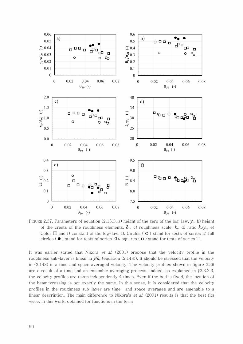
90

0

0.01

0.02

0.03

0.04

0.05

0.06

0 0.02 0.04 0.06 0.08θ50 (-)

y a/d

90

(-)

0

0.1

0.2

0.3

0.4

0.5

0.6

0 0.02 0.04 0.06 0.08θ50 (-)

¬ a/d

90

(-)

0.0

0.5

1.0

1.5

2.0

0 0.02 0.04 0.06 0.08θ50 (-)

k s/d

90

(-)

20

25

30

35

40

0 0.02 0.04 0.06 0.08θ50 (-)

k s/y

a

(-)

0

0.1

0.2

0.3

0.4

0 0.02 0.04 0.06 0.08θ50 (-)

ℵ

(-)

7.5

8.0

8.5

9.0

9.5

0 0.02 0.04 0.06 0.08θ50 (-)

B

(-)

FIGURE 2.37. Parameters of equation (2.151). a) height of the zero of the log-law, ya, b) height

of the crests of the roughness elements, δa, c) roughness scale, ks, d) ratio ks/ya, e)

Coles Π and f) constant of the log-law, B. Circles ( ) stand for tests of series E; full

circles ( ) stand for tests of series ED; squares ( ) stand for tests of series T.

It was earlier stated that Nikora et al. (2001) propose that the velocity profile in the

roughness sub-layer is linear in y/ks (equation (2.148)). It should be stressed that the velocity

in (2.148) is a time and space averaged velocity. The velocity profiles shown in figure 2.39

are a result of a time and an ensemble averaging process. Indeed, as explained in §2.3.2.3,

the velocity profiles are taken independently 4 times. Even if the bed is fixed, the location of

the beam-crossing is not exactly the same. In this sense, it is considered that the velocity

profiles in the roughness sub-layer are time- and space-averages and are amenable to a

linear description. The main difference to Nikora’s et al. (2001) results is that the best fits

were, in this work, obtained for functions in the form

a) b)

c) d)

e) f)

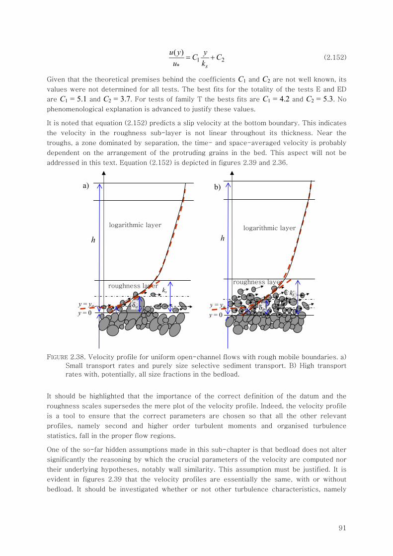
91

1 2*

( )

s

u y yC Cu k

= + (2.152)

Given that the theoretical premises behind the coefficients C1 and C2 are not well known, its

values were not determined for all tests. The best fits for the totality of the tests E and ED

are C1 = 5.1 and C2 = 3.7. For tests of family T the bests fits are C1 = 4.2 and C2 = 5.3. No

phenomenological explanation is advanced to justify these values.

It is noted that equation (2.152) predicts a slip velocity at the bottom boundary. This indicates

the velocity in the roughness sub-layer is not linear throughout its thickness. Near the

troughs, a zone dominated by separation, the time- and space-averaged velocity is probably

dependent on the arrangement of the protruding grains in the bed. This aspect will not be

addressed in this text. Equation (2.152) is depicted in figures 2.39 and 2.36.

FIGURE 2.38. Velocity profile for uniform open-channel flows with rough mobile boundaries. a)

Small transport rates and purely size selective sediment transport. B) High transport

rates with, potentially, all size fractions in the bedload.

It should be highlighted that the importance of the correct definition of the datum and the

roughness scales supersedes the mere plot of the velocity profile. Indeed, the velocity profile

is a tool to ensure that the correct parameters are chosen so that all the other relevant

profiles, namely second and higher order turbulent moments and organised turbulence

statistics, fall in the proper flow regions.

One of the so-far hidden assumptions made in this sub-chapter is that bedload does not alter

significantly the reasoning by which the crucial parameters of the velocity are computed nor

their underlying hypotheses, notably wall similarity. This assumption must be justified. It is

evident in figures 2.39 that the velocity profiles are essentially the same, with or without

bedload. It should be investigated whether or not other turbulence characteristics, namely

logarithmic layer

roughness layer

δay = 0 y = ya

ks

h

roughness layer

logarithmic layer

y = 0 y = ya

ks

δa

h

a) b)

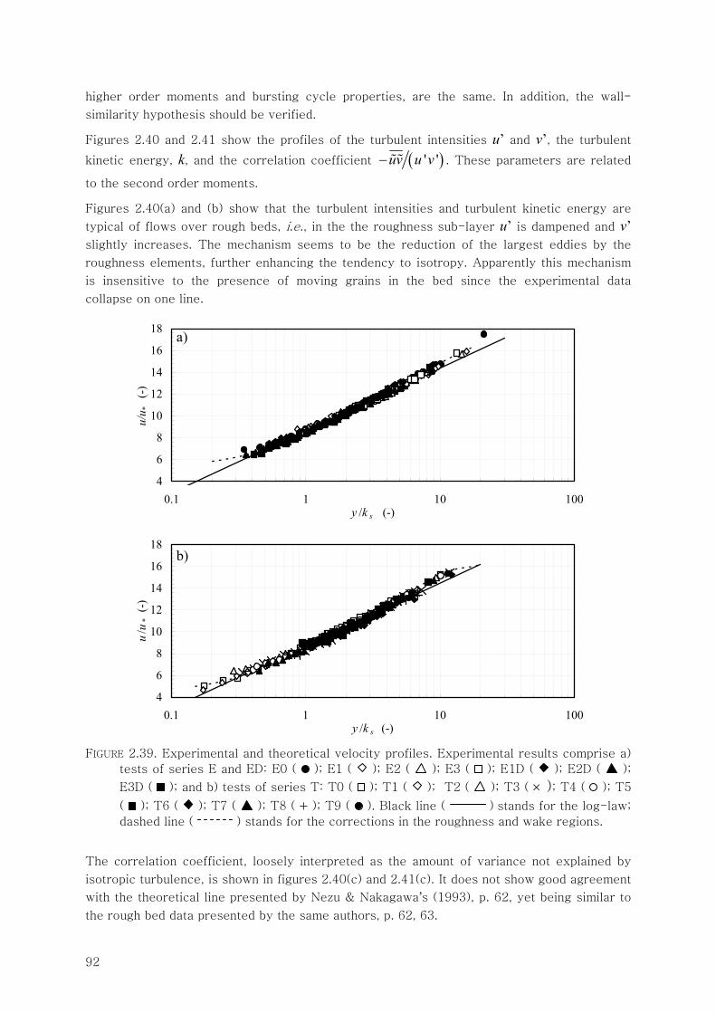
92

higher order moments and bursting cycle properties, are the same. In addition, the wall-

similarity hypothesis should be verified.

Figures 2.40 and 2.41 show the profiles of the turbulent intensities u’ and v’, the turbulent

kinetic energy, k, and the correlation coefficient ( )' 'uv u v− . These parameters are related

to the second order moments.

Figures 2.40(a) and (b) show that the turbulent intensities and turbulent kinetic energy are

typical of flows over rough beds, i.e., in the the roughness sub-layer u’ is dampened and v’ slightly increases. The mechanism seems to be the reduction of the largest eddies by the

roughness elements, further enhancing the tendency to isotropy. Apparently this mechanism

is insensitive to the presence of moving grains in the bed since the experimental data

collapse on one line.

4

6

8

10

12

14

16

18

0.1 1 10 100y /k s (-)

u/u *

(-)

4

6

8

10

12

14

16

18

0.1 1 10 100y /k s (-)

u/u

* (-

)

FIGURE 2.39. Experimental and theoretical velocity profiles. Experimental results comprise a)

tests of series E and ED: E0 ( ); E1 ( ); E2 ( ); E3 ( ); E1D ( ); E2D ( );

E3D ( ); and b) tests of series T: T0 ( ); T1 ( ); T2 ( ); T3 ( × ); T4 ( ); T5

( ); T6 ( ); T7 ( ); T8 ( + ); T9 ( ). Black line ( ) stands for the log-law;

dashed line ( ) stands for the corrections in the roughness and wake regions.

The correlation coefficient, loosely interpreted as the amount of variance not explained by

isotropic turbulence, is shown in figures 2.40(c) and 2.41(c). It does not show good agreement

with the theoretical line presented by Nezu & Nakagawa’s (1993), p. 62, yet being similar to

the rough bed data presented by the same authors, p. 62, 63.

a)

b)

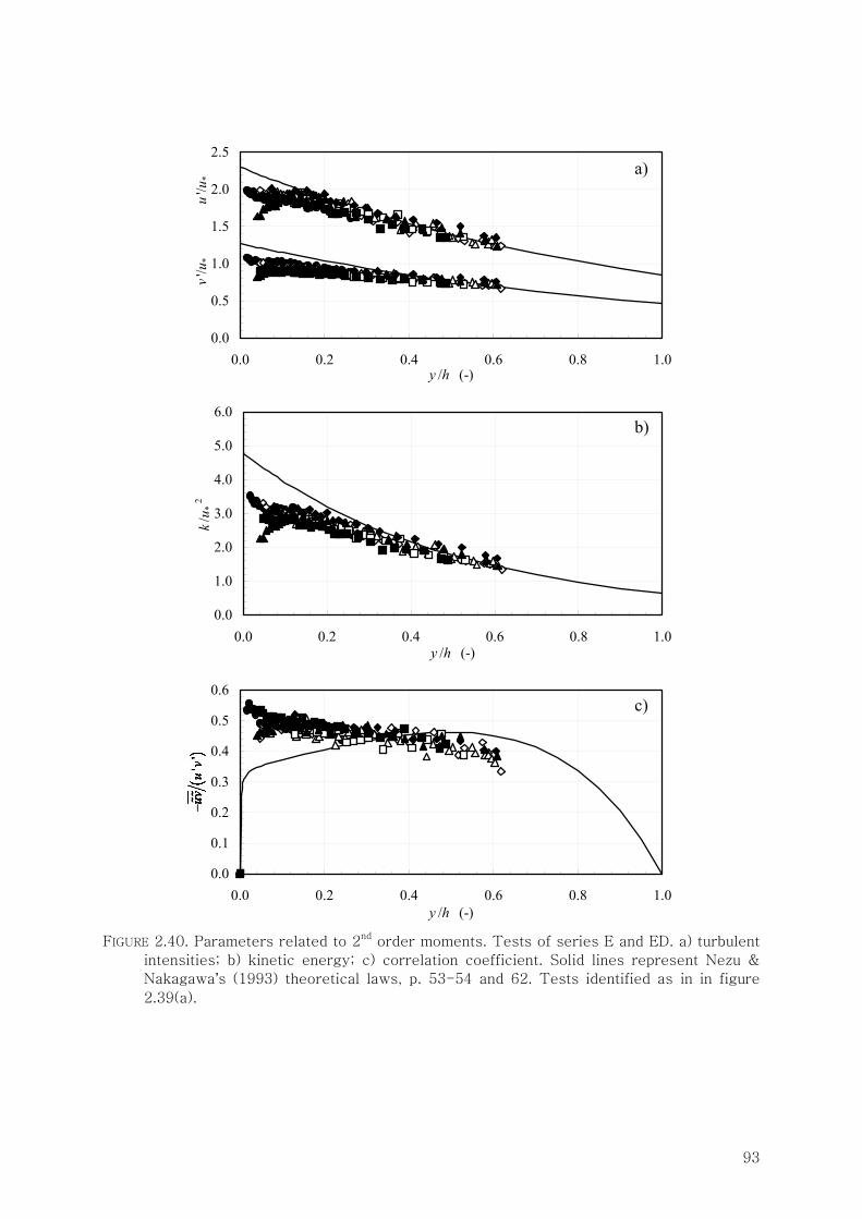
93

0.0

0.5

1.0

1.5

2.0

2.5

0.0 0.2 0.4 0.6 0.8 1.0y /h (-)

v

'/u*

u'/u

*

0.0

1.0

2.0

3.0

4.0

5.0

6.0

0.0 0.2 0.4 0.6 0.8 1.0y /h (-)

k/u *

2

0.0

0.1

0.2

0.3

0.4

0.5

0.6

0.0 0.2 0.4 0.6 0.8 1.0y /h (-)

-uv/

(u'v

')

FIGURE 2.40. Parameters related to 2nd order moments. Tests of series E and ED. a) turbulent

intensities; b) kinetic energy; c) correlation coefficient. Solid lines represent Nezu &

Nakagawa’s (1993) theoretical laws, p. 53-54 and 62. Tests identified as in in figure

2.39(a).

a)

b)

c)

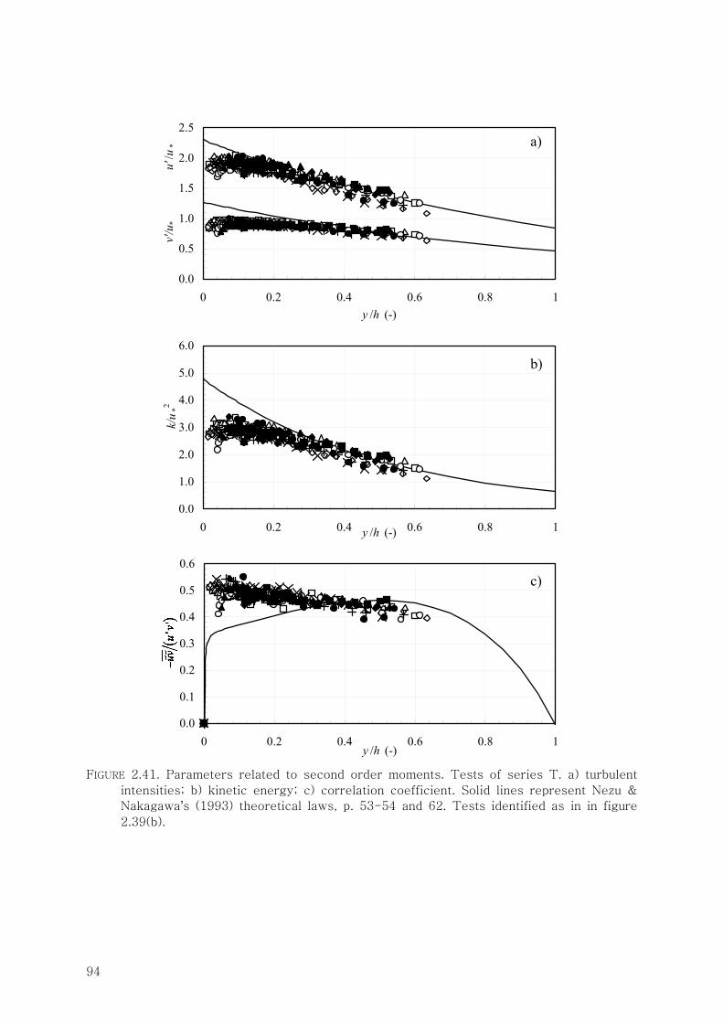
94

0.0

0.5

1.0

1.5

2.0

2.5

0 0.2 0.4 0.6 0.8 1y /h (-)

v'/u

*

u'

/u*

0.0

1.0

2.0

3.0

4.0

5.0

6.0

0 0.2 0.4 0.6 0.8 1y /h (-)

k/u

*2

0.0

0.1

0.2

0.3

0.4

0.5

0.6

0 0.2 0.4 0.6 0.8 1y /h (-)

uv/(

u'v

')

FIGURE 2.41. Parameters related to second order moments. Tests of series T. a) turbulent

intensities; b) kinetic energy; c) correlation coefficient. Solid lines represent Nezu &

Nakagawa’s (1993) theoretical laws, p. 53-54 and 62. Tests identified as in in figure

2.39(b).

a)

b)

c)

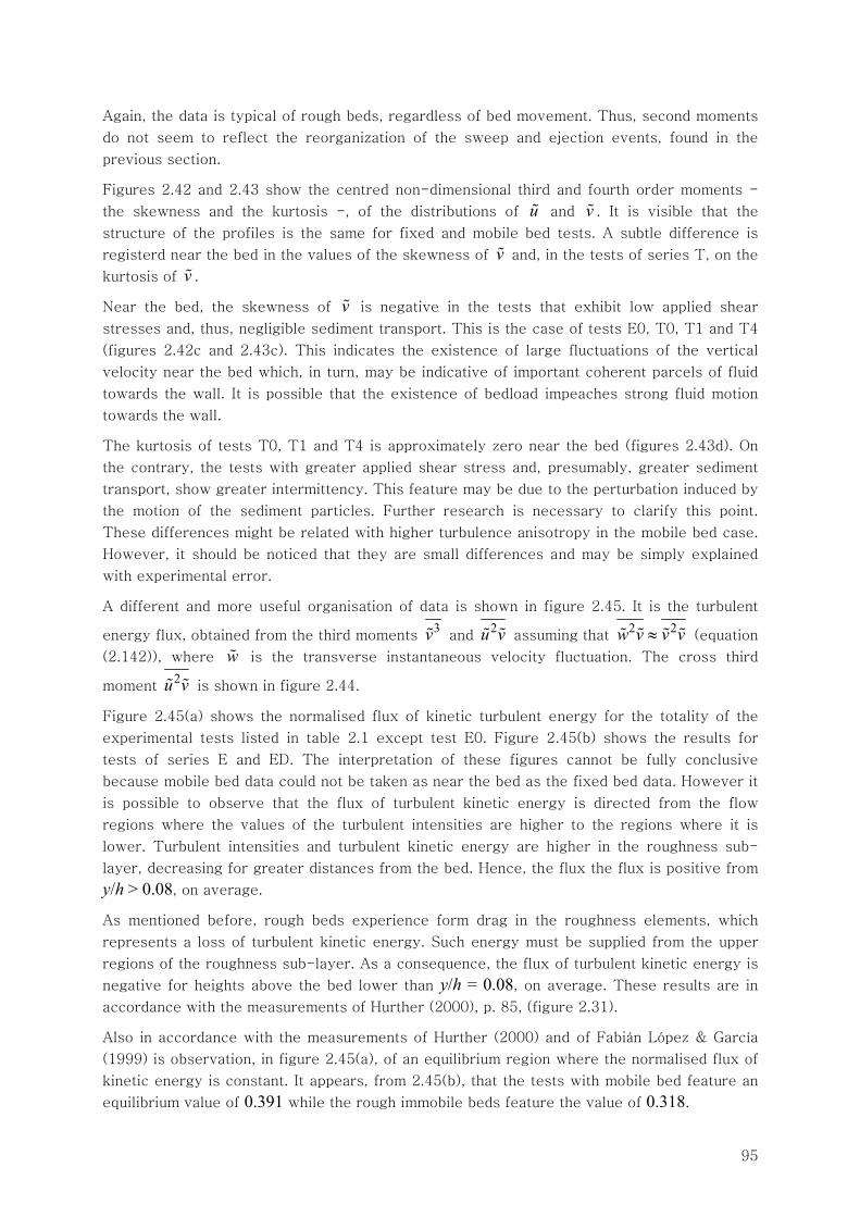
95

Again, the data is typical of rough beds, regardless of bed movement. Thus, second moments

do not seem to reflect the reorganization of the sweep and ejection events, found in the

previous section.

Figures 2.42 and 2.43 show the centred non-dimensional third and fourth order moments -

the skewness and the kurtosis -, of the distributions of u and v . It is visible that the

structure of the profiles is the same for fixed and mobile bed tests. A subtle difference is

registerd near the bed in the values of the skewness of v and, in the tests of series T, on the

kurtosis of v .

Near the bed, the skewness of v is negative in the tests that exhibit low applied shear

stresses and, thus, negligible sediment transport. This is the case of tests E0, T0, T1 and T4

(figures 2.42c and 2.43c). This indicates the existence of large fluctuations of the vertical

velocity near the bed which, in turn, may be indicative of important coherent parcels of fluid

towards the wall. It is possible that the existence of bedload impeaches strong fluid motion

towards the wall.

The kurtosis of tests T0, T1 and T4 is approximately zero near the bed (figures 2.43d). On

the contrary, the tests with greater applied shear stress and, presumably, greater sediment

transport, show greater intermittency. This feature may be due to the perturbation induced by

the motion of the sediment particles. Further research is necessary to clarify this point.

These differences might be related with higher turbulence anisotropy in the mobile bed case.

However, it should be noticed that they are small differences and may be simply explained

with experimental error.

A different and more useful organisation of data is shown in figure 2.45. It is the turbulent

energy flux, obtained from the third moments 3v and

2u v assuming that 2 2w v v v≈ (equation

(2.142)), where w is the transverse instantaneous velocity fluctuation. The cross third

moment 2u v is shown in figure 2.44.

Figure 2.45(a) shows the normalised flux of kinetic turbulent energy for the totality of the

experimental tests listed in table 2.1 except test E0. Figure 2.45(b) shows the results for

tests of series E and ED. The interpretation of these figures cannot be fully conclusive

because mobile bed data could not be taken as near the bed as the fixed bed data. However it

is possible to observe that the flux of turbulent kinetic energy is directed from the flow

regions where the values of the turbulent intensities are higher to the regions where it is

lower. Turbulent intensities and turbulent kinetic energy are higher in the roughness sub-

layer, decreasing for greater distances from the bed. Hence, the flux the flux is positive from

y/h > 0.08, on average.

As mentioned before, rough beds experience form drag in the roughness elements, which

represents a loss of turbulent kinetic energy. Such energy must be supplied from the upper

regions of the roughness sub-layer. As a consequence, the flux of turbulent kinetic energy is

negative for heights above the bed lower than y/h = 0.08, on average. These results are in

accordance with the measurements of Hurther (2000), p. 85, (figure 2.31).

Also in accordance with the measurements of Hurther (2000) and of Fabián López & García

(1999) is observation, in figure 2.45(a), of an equilibrium region where the normalised flux of

kinetic energy is constant. It appears, from 2.45(b), that the tests with mobile bed feature an

equilibrium value of 0.391 while the rough immobile beds feature the value of 0.318.

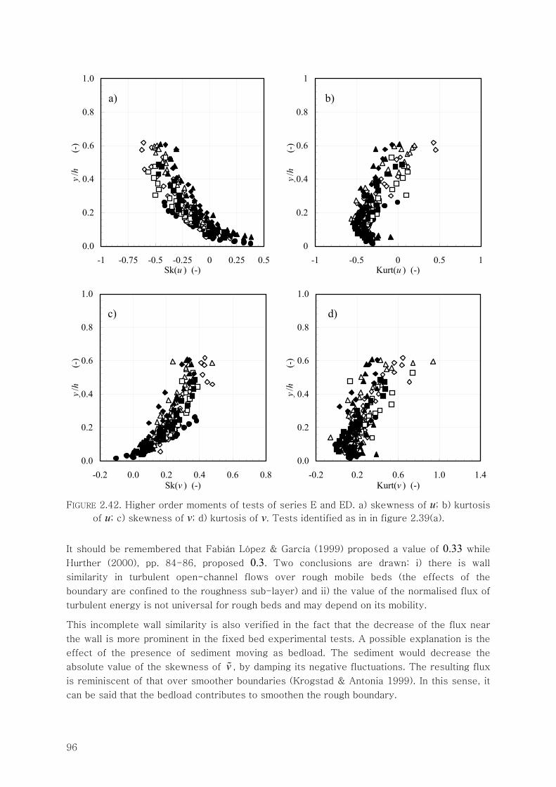
96

0.0

0.2

0.4

0.6

0.8

1.0

-1 -0.75 -0.5 -0.25 0 0.25 0.5Sk(u ) (-)

y/h

(-)

0

0.2

0.4

0.6

0.8

1

-1 -0.5 0 0.5 1Kurt(u ) (-)

y/h

(-)

0.0

0.2

0.4

0.6

0.8

1.0

-0.2 0.0 0.2 0.4 0.6 0.8Sk(v ) (-)

y/h

(-)

0.0

0.2

0.4

0.6

0.8

1.0

-0.2 0.2 0.6 1.0 1.4Kurt(v ) (-)

y/h

(-)

FIGURE 2.42. Higher order moments of tests of series E and ED. a) skewness of u; b) kurtosis

of u; c) skewness of v; d) kurtosis of v. Tests identified as in in figure 2.39(a).

It should be remembered that Fabián López & García (1999) proposed a value of 0.33 while

Hurther (2000), pp. 84-86, proposed 0.3. Two conclusions are drawn: i) there is wall

similarity in turbulent open-channel flows over rough mobile beds (the effects of the

boundary are confined to the roughness sub-layer) and ii) the value of the normalised flux of

turbulent energy is not universal for rough beds and may depend on its mobility.

This incomplete wall similarity is also verified in the fact that the decrease of the flux near

the wall is more prominent in the fixed bed experimental tests. A possible explanation is the

effect of the presence of sediment moving as bedload. The sediment would decrease the

absolute value of the skewness of v , by damping its negative fluctuations. The resulting flux

is reminiscent of that over smoother boundaries (Krogstad & Antonia 1999). In this sense, it

can be said that the bedload contributes to smoothen the rough boundary.

a) b)

c) d)

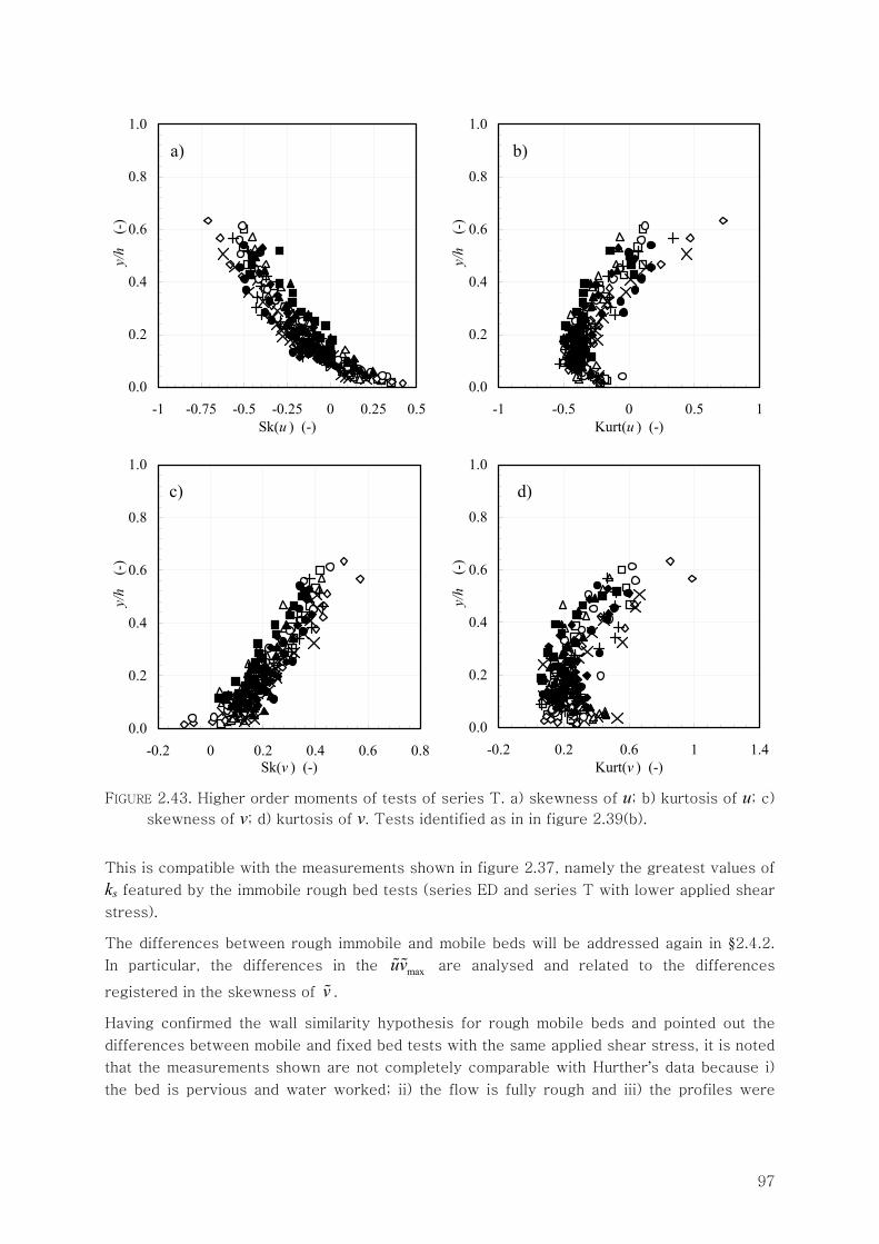
97

0.0

0.2

0.4

0.6

0.8

1.0

-1 -0.75 -0.5 -0.25 0 0.25 0.5Sk(u ) (-)

y/h

(-

)

0.0

0.2

0.4

0.6

0.8

1.0

-1 -0.5 0 0.5 1Kurt(u ) (-)

y/h

(-

)

0.0

0.2

0.4

0.6

0.8

1.0

-0.2 0 0.2 0.4 0.6 0.8Sk(v ) (-)

y/h

(-

)

0.0

0.2

0.4

0.6

0.8

1.0

-0.2 0.2 0.6 1 1.4Kurt(v ) (-)

y/h

(-

)

FIGURE 2.43. Higher order moments of tests of series T. a) skewness of u; b) kurtosis of u; c)

skewness of v; d) kurtosis of v. Tests identified as in in figure 2.39(b).

This is compatible with the measurements shown in figure 2.37, namely the greatest values of

ks featured by the immobile rough bed tests (series ED and series T with lower applied shear

stress).

The differences between rough immobile and mobile beds will be addressed again in §2.4.2.

In particular, the differences in the maxuv are analysed and related to the differences

registered in the skewness of v .

Having confirmed the wall similarity hypothesis for rough mobile beds and pointed out the

differences between mobile and fixed bed tests with the same applied shear stress, it is noted

that the measurements shown are not completely comparable with Hurther’s data because i)

the bed is pervious and water worked; ii) the flow is fully rough and iii) the profiles were

a) b)

c) d)

98

measured with LDA, thus pointwise, each taking about two hours to perform. Consequently,

data scattering is much larger in the measurements shown in this sub-chapter.

-0.8

-0.4

0.0

0.4

0.8

0.0 0.2 0.4 0.6 0.8 1.0y /h (-)

u2 v/

u *3

(-)

-0.8

-0.4

0.0

0.4

0.8

0 0.2 0.4 0.6 0.8 1y /h (-)

u

2 v/u

*3

FIGURE 2.44. Third order moment 2 3

*u v u . a) Tests of series E and ED; b) tests of series T.

Tests identified as in in figure 2.39.

Figure 2.46 shows the production and the turbulent diffusion terms of the equation of

conservation of turbulent kinetic energy, terms E and D1, respectively, in equation (2.141).

The turbulent production is clearly unaffected by the type of boundary, mobile or immobile.

The turbulent diffusion, TD, was obtained from differentiation of the turbulent flux. Given the

scatter of the latter, the data was previously smoothened by a moving average process. It is

clear that the values of TD are greater near the bed in the fixed bed tests (series ED and T0,

T1, T2 and T4) than in the mobile bed tests. This increased gradient of the flux is a

consequence of its negative values in the fixed bed tests.

The remaining terms of the equation of conservation of turbulent kinetic energy, equation

(2.141), can be determined if a spectral analysis to the instantaneous velocity series is

carried out.

The wall, intermediate and free-surface regions are loosely connected with the production,

inertial and dissipation uu spectral sub-ranges. Figure 2.47 shows the normalized uu spectral

function as well as the dissipation spectrum as a function of the wave number, kx, in the

stream-wise direction. The spectrum of u is given by

112( ) ( ) de xik

x uuS k r+∞

− ξ

−∞

= ξ ξπ ∫ (2.153)

a)

b)

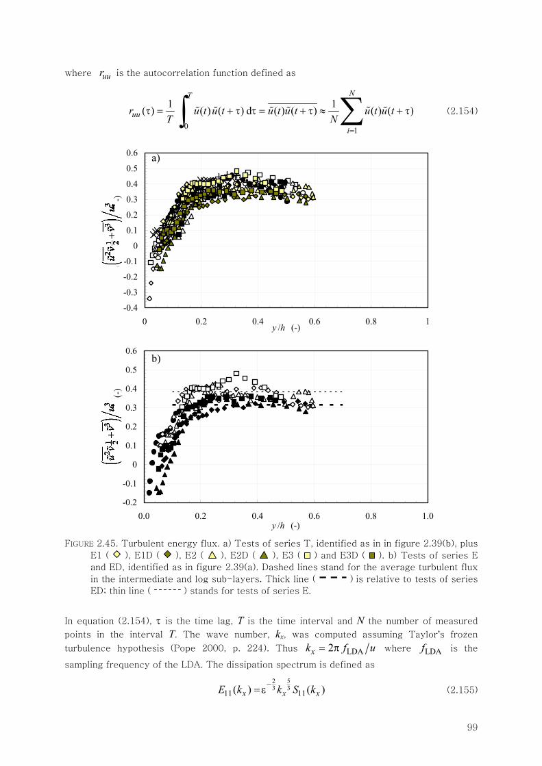
99

where uur is the autocorrelation function defined as

0 1

1 1( ) ( ) ( ) d ( ) ( ) ( ) ( )

NT

uu

i

r u t u t u t u t u t u tT N

=

τ = + τ τ = + τ ≈ + τ∑∫ (2.154)

-0.4

-0.3

-0.2

-0.1

0

0.1

0.2

0.3

0.4

0.5

0.6

0 0.2 0.4 0.6 0.8 1y /h (-)

(u2 v/

2+v3 )/u

*3

(-)

-0.2

-0.1

0

0.1

0.2

0.3

0.4

0.5

0.6

0.0 0.2 0.4 0.6 0.8 1.0y /h (-)

(u2 v/

2 +

v3 )/u*

3 (-)

FIGURE 2.45. Turbulent energy flux. a) Tests of series T, identified as in in figure 2.39(b), plus

E1 ( ), E1D ( ), E2 ( ), E2D ( ), E3 ( ) and E3D ( ). b) Tests of series E

and ED, identified as in figure 2.39(a). Dashed lines stand for the average turbulent flux

in the intermediate and log sub-layers. Thick line ( ) is relative to tests of series

ED; thin line ( ) stands for tests of series E.

In equation (2.154), τ is the time lag, T is the time interval and N the number of measured

points in the interval T. The wave number, kx, was computed assuming Taylor’s frozen

turbulence hypothesis (Pope 2000, p. 224). Thus LDA2xk f u= π where LDAf is the

sampling frequency of the LDA. The dissipation spectrum is defined as

52

3 311 11( ) ( )x x xE k k S k−

= ε (2.155)

a)

b)

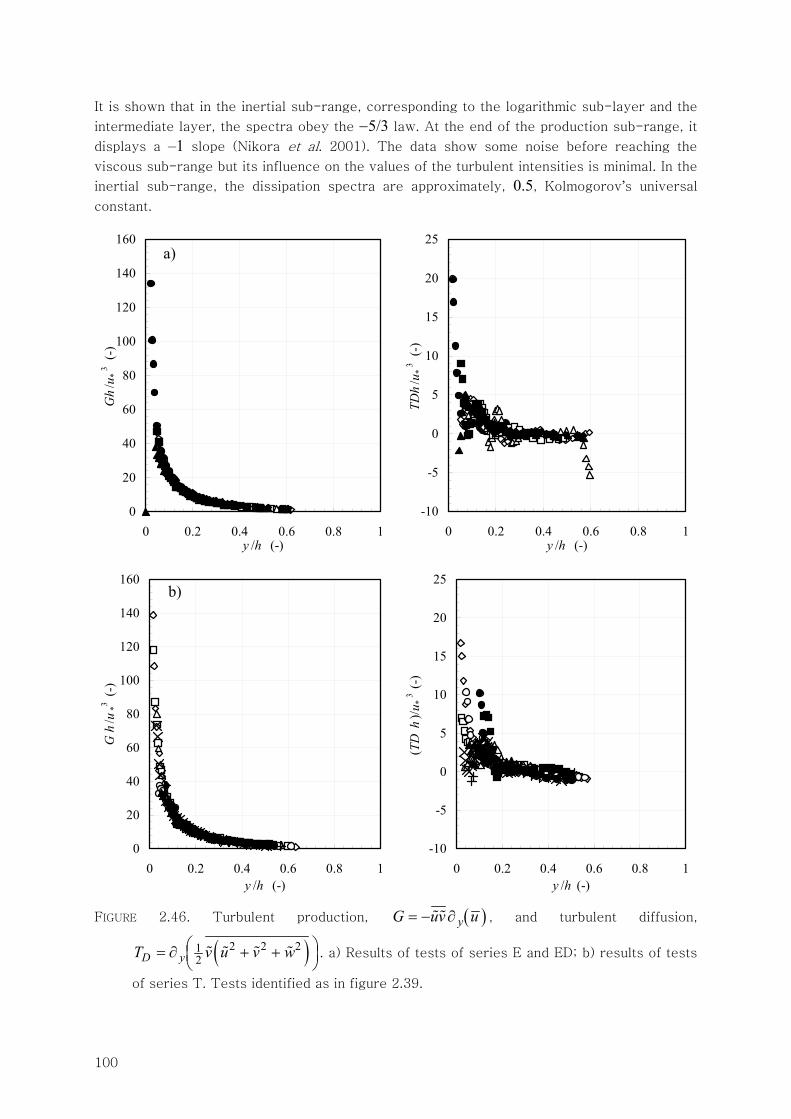
100

It is shown that in the inertial sub-range, corresponding to the logarithmic sub-layer and the

intermediate layer, the spectra obey the −5/3 law. At the end of the production sub-range, it

displays a –1 slope (Nikora et al. 2001). The data show some noise before reaching the

viscous sub-range but its influence on the values of the turbulent intensities is minimal. In the

inertial sub-range, the dissipation spectra are approximately, 0.5, Kolmogorov’s universal

constant.

0

20

40

60

80

100

120

140

160

0 0.2 0.4 0.6 0.8 1y /h (-)

Gh

/u*

3 (-)

-10

-5

0

5

10

15

20

25

0 0.2 0.4 0.6 0.8 1y /h (-)

TDh

/u*

3 (-)

0

20

40

60

80

100

120

140

160

0 0.2 0.4 0.6 0.8 1y /h (-)

G h

/u*3

(-)

-10

-5

0

5

10

15

20

25

0 0.2 0.4 0.6 0.8 1y /h (-)

(TD

h)/u

*3

(-)

FIGURE 2.46. Turbulent production, ( )yG uv u= − ∂ , and turbulent diffusion,

( )2 2 212D yT v u v w⎛ ⎞= ∂ + +⎜ ⎟

⎝ ⎠. a) Results of tests of series E and ED; b) results of tests

of series T. Tests identified as in figure 2.39.

a)

b)

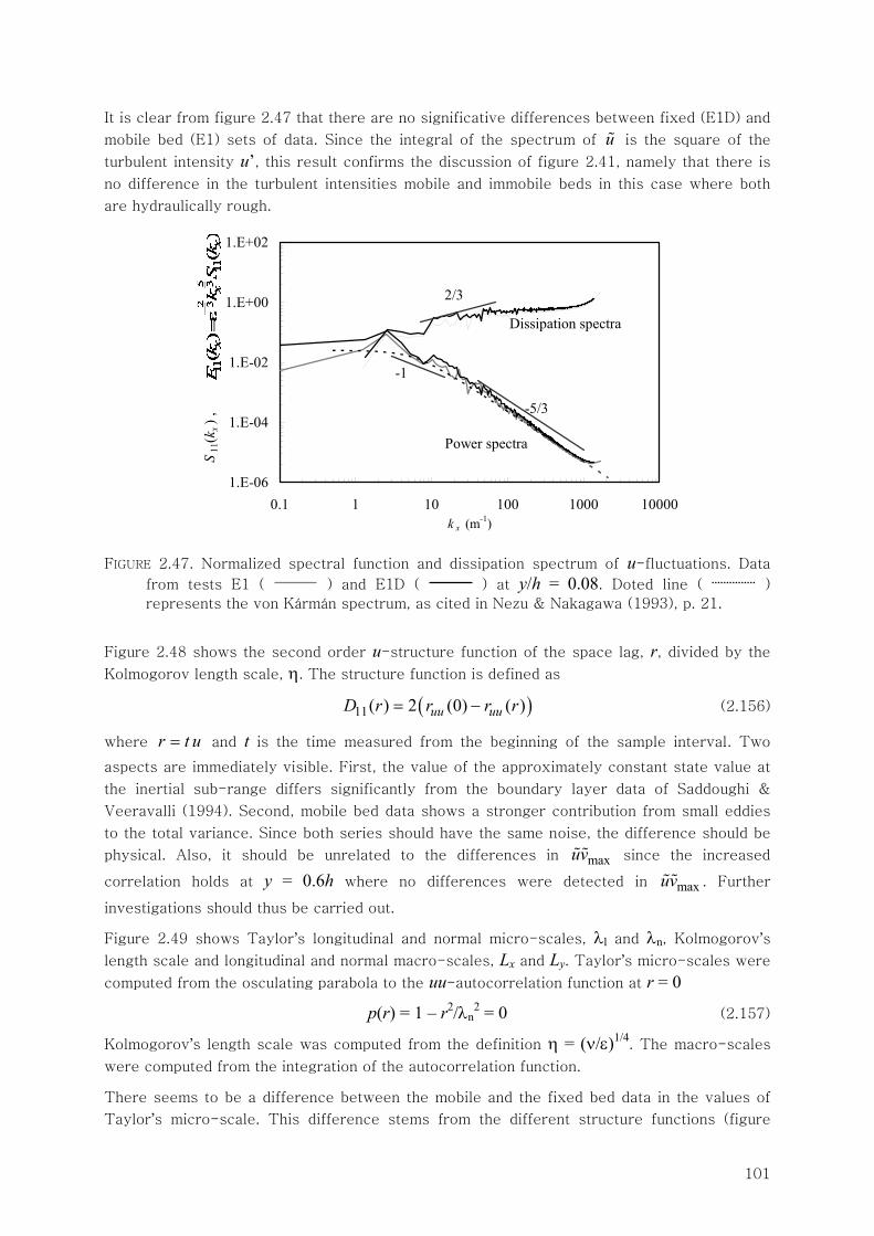
101

It is clear from figure 2.47 that there are no significative differences between fixed (E1D) and

mobile bed (E1) sets of data. Since the integral of the spectrum of u is the square of the

turbulent intensity u’, this result confirms the discussion of figure 2.41, namely that there is

no difference in the turbulent intensities mobile and immobile beds in this case where both

are hydraulically rough.

1.E-06

1.E-04

1.E-02

1.E+00

1.E+02

0.1 1 10 100 1000 10000k x (m-1)

S11

(kx) ,

kx

5/3 ℵ-2

/3S

11(k

x)

-5/3

-1

2/3

Dissipation spectra

Power spectra

FIGURE 2.47. Normalized spectral function and dissipation spectrum of u-fluctuations. Data

from tests E1 ( ) and E1D ( ) at y/h = 0.08. Doted line ( )

represents the von Kármán spectrum, as cited in Nezu & Nakagawa (1993), p. 21.

Figure 2.48 shows the second order u-structure function of the space lag, r, divided by the

Kolmogorov length scale, η. The structure function is defined as

( )11( ) 2 (0) ( )uu uuD r r r r= − (2.156)

where r t u= and t is the time measured from the beginning of the sample interval. Two

aspects are immediately visible. First, the value of the approximately constant state value at

the inertial sub-range differs significantly from the boundary layer data of Saddoughi &

Veeravalli (1994). Second, mobile bed data shows a stronger contribution from small eddies

to the total variance. Since both series should have the same noise, the difference should be

physical. Also, it should be unrelated to the differences in maxuv since the increased

correlation holds at y = 0.6h where no differences were detected in maxuv . Further

investigations should thus be carried out.

Figure 2.49 shows Taylor’s longitudinal and normal micro-scales, λl and λn, Kolmogorov’s

length scale and longitudinal and normal macro-scales, Lx and Ly. Taylor’s micro-scales were

computed from the osculating parabola to the uu-autocorrelation function at r = 0

p(r) = 1 – r2/λn2 = 0 (2.157)

Kolmogorov’s length scale was computed from the definition η = (ν/ε)1/4. The macro-scales

were computed from the integration of the autocorrelation function.

There seems to be a difference between the mobile and the fixed bed data in the values of

Taylor’s micro-scale. This difference stems from the different structure functions (figure

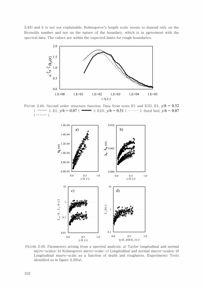
102

2.48) and it is not yet explainable. Kolmogorov’s length scale seems to depend only on the

Reynolds number and not on the nature of the boundary, which is in agreement with the

spectral data. The values are within the expected limits for rough boundaries.

0.0

0.5

1.0

1.5

2.0

1.E+00 1.E+01 1.E+02 1.E+03 1.E+04 1.E+05r /η (-)

ℵ-2/3

r-2/3

D11

(r)

FIGURE 2.48. Second order structure function. Data from tests E1 and E1D. E1, y/h = 0.52

( ); E1, y/h = 0.07 ( ); E1D, y/h = 0.51 ( ); fixed bed, y/h = 0.07

( ).

6.0E-05

8.0E-05

1.0E-04

1.2E-04

1.4E-04

1.6E-04

0.0 0.5 1.0y /h (-)

ℵ L (m

)

0.000

0.005

0.010

0.0 0.5 1.0y /h (-)

ℵ l ,

ℵn (

m)

0.01

0.1

1

10

0.0 0.5 1.0y /h (-)

Lx,/

h,

Ly /

h (-

)

0.1

1

10

0.0 0.5 1.0(y-k s )/(h-k s ) (-)

Lx/h

(-)

FIGURE 2.49. Parameters arising from a spectral analysis. a) Taylor longitudinal and normal

micro-scales; b) Kolmogorov micro-scale; c) Longitudinal and normal macro-scales; d)

Longitudinal macro-scale as a function of depth and roughness. Experiments Tests

identified as in figure 2.39(a).

a) b)

c) d)

103

The longitudinal and normal macro-scales do not seem do depend on the bed movement,

which is in agreement with the fact that turbulent intensities also do not display any

differences. In fact, turbulent intensities are similar as a consequence of the similarity in the

macro-scales. Special attention should be paid to figure 2.49(d). This particular choice of axis

enhances the visibility of the roughness influence of the longitudinal macro-scale. Again, the

mobile bed data is indiscernible from the fixed bed.

Having computed Taylor micro-scales, the dissipation rate can be computed. Figure 2.50

shows the turbulent energy budget. The dissipation rate was obtained from

215 'n uλ = υ ε (2.158)

where λn is the normal Taylor micro-scale and ε is total turbulent dissipation.

The pressure diffusion term was computed as PD = G – ε – TD (where G is the turbulent

production) under the hypothesis that viscous diffusion is negligible. The production and

dissipation terms appear to be independent from the boundary conditions and Reynolds

number.

-10

0

10

20

30

40

50

0.01 0.1 1y /h (-)

ℵ h

/u*3 ,

G h

/u*3 ,

TDh

/u*3 ,

P Dh

/u*3

E mobile

E fixed

G mobile

G fixed

TD mobile

PD mobile

TD fixed

PD fixed

FIGURE 2.50. Turbulent energy budget for Tests E1 and E1D.

It can be seen in figure 2.50 that, in the wall region (approximatelly y < 0.2h), G > ε, i.e.,

turbulence is generated. Production and dissipation are in equilibrium in the intermediate

region. In the free-surface region (y > 0.6h) G < ε, i.e., energy is mostly dissipated. The

computed values of G and ε are, thus, in accordance with the observed behaviour in open-

channel flows over rough or smooth beds (see, e.g., Townsend 1976, p. 145).

As for the remaining terms, the order of magnitude seems correct, but no further

interpretations should be made since the hypothesis admitted for their computation render the

values somewhat imprecise.

The series of tests identified in 2.1 all feature hidraulically rough beds. The analysis carried

out above shows that, for these rough beds, the differences between mobile and immobile

beds are subtle and confined to higher order moments. Nikora & Goring (2000) believed that

ε

ε

G

G

DT

DT

DP

DP

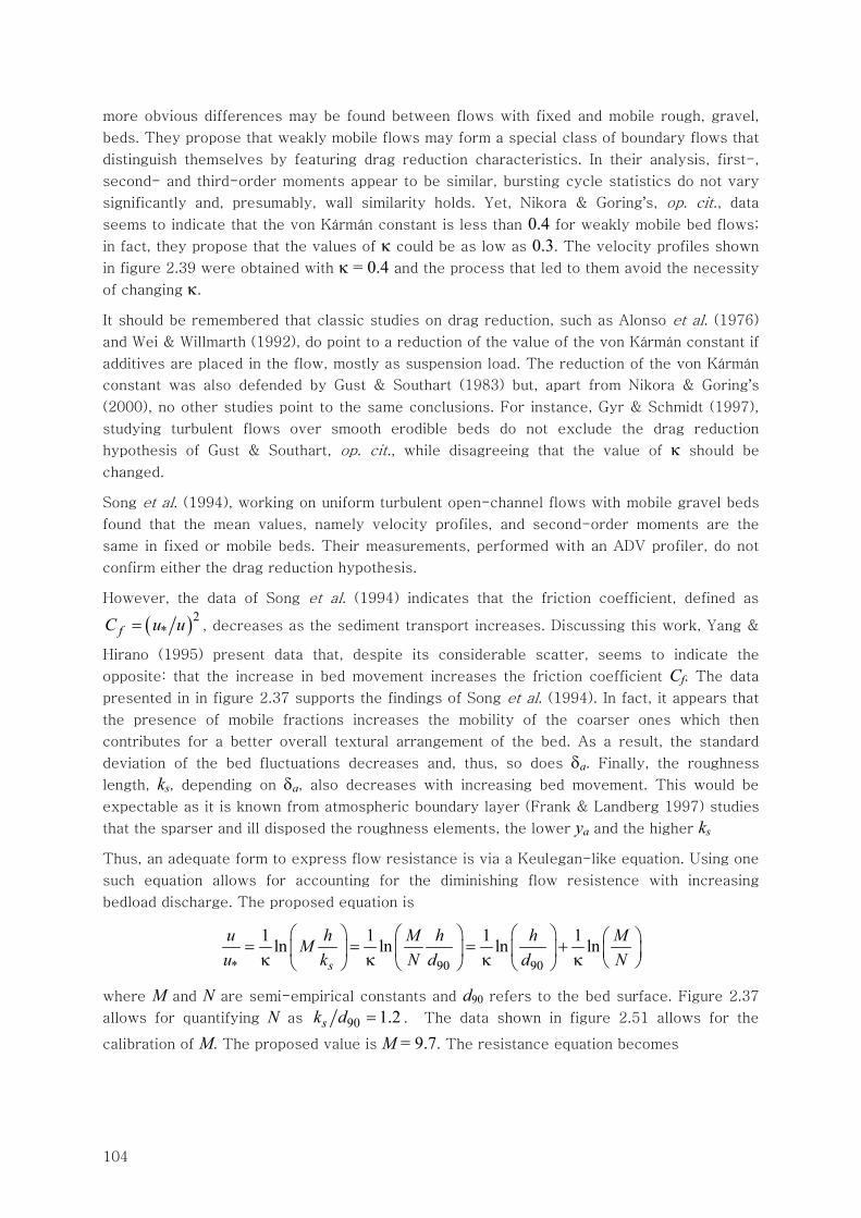
104

more obvious differences may be found between flows with fixed and mobile rough, gravel,

beds. They propose that weakly mobile flows may form a special class of boundary flows that

distinguish themselves by featuring drag reduction characteristics. In their analysis, first-,

second- and third-order moments appear to be similar, bursting cycle statistics do not vary

significantly and, presumably, wall similarity holds. Yet, Nikora & Goring’s, op. cit., data

seems to indicate that the von Kármán constant is less than 0.4 for weakly mobile bed flows;

in fact, they propose that the values of κ could be as low as 0.3. The velocity profiles shown

in figure 2.39 were obtained with κ = 0.4 and the process that led to them avoid the necessity

of changing κ.

It should be remembered that classic studies on drag reduction, such as Alonso et al. (1976)

and Wei & Willmarth (1992), do point to a reduction of the value of the von Kármán constant if

additives are placed in the flow, mostly as suspension load. The reduction of the von Kármán

constant was also defended by Gust & Southart (1983) but, apart from Nikora & Goring’s

(2000), no other studies point to the same conclusions. For instance, Gyr & Schmidt (1997),

studying turbulent flows over smooth erodible beds do not exclude the drag reduction

hypothesis of Gust & Southart, op. cit., while disagreeing that the value of κ should be

changed.

Song et al. (1994), working on uniform turbulent open-channel flows with mobile gravel beds

found that the mean values, namely velocity profiles, and second-order moments are the

same in fixed or mobile beds. Their measurements, performed with an ADV profiler, do not

confirm either the drag reduction hypothesis.

However, the data of Song et al. (1994) indicates that the friction coefficient, defined as

( )2*fC u u= , decreases as the sediment transport increases. Discussing this work, Yang &

Hirano (1995) present data that, despite its considerable scatter, seems to indicate the

opposite: that the increase in bed movement increases the friction coefficient Cf. The data

presented in in figure 2.37 supports the findings of Song et al. (1994). In fact, it appears that

the presence of mobile fractions increases the mobility of the coarser ones which then

contributes for a better overall textural arrangement of the bed. As a result, the standard

deviation of the bed fluctuations decreases and, thus, so does δa. Finally, the roughness

length, ks, depending on δa, also decreases with increasing bed movement. This would be

expectable as it is known from atmospheric boundary layer (Frank & Landberg 1997) studies

that the sparser and ill disposed the roughness elements, the lower ya and the higher ks

Thus, an adequate form to express flow resistance is via a Keulegan-like equation. Using one

such equation allows for accounting for the diminishing flow resistence with increasing

bedload discharge. The proposed equation is

* 90 90

1 1 1 1ln ln ln lns

u h M h h MMu k N d d N

⎛ ⎞ ⎛ ⎞ ⎛ ⎞ ⎛ ⎞= = = +⎜ ⎟ ⎜ ⎟ ⎜ ⎟ ⎜ ⎟κ κ κ κ ⎝ ⎠⎝ ⎠ ⎝ ⎠ ⎝ ⎠

where M and N are semi-empirical constants and d90 refers to the bed surface. Figure 2.37

allows for quantifying N as 90 1.2sk d = . The data shown in figure 2.51 allows for the

calibration of M. The proposed value is M = 9.7. The resistance equation becomes

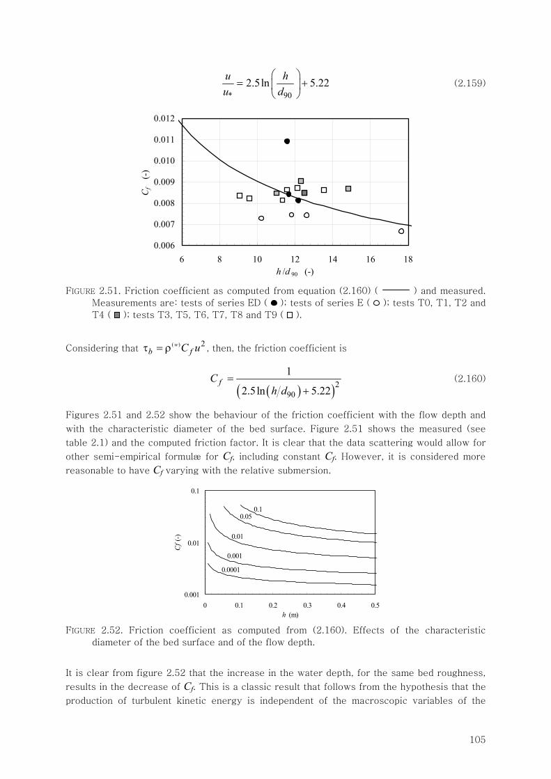
105

* 90

2.5ln 5.22u hu d

⎛ ⎞= +⎜ ⎟

⎝ ⎠ (2.159)

0.006

0.007

0.008

0.009

0.010

0.011

0.012

6 8 10 12 14 16 18h /d 90 (-)

C f

(-)

FIGURE 2.51. Friction coefficient as computed from equation (2.160) ( ) and measured.

Measurements are: tests of series ED ( ); tests of series E ( ); tests T0, T1, T2 and

T4 ( ); tests T3, T5, T6, T7, T8 and T9 ( ).

Considering that ( ) 2w

b fC uτ = ρ , then, the friction coefficient is

( )( )290

1

2.5ln 5.22fC

h d=

+ (2.160)

Figures 2.51 and 2.52 show the behaviour of the friction coefficient with the flow depth and

with the characteristic diameter of the bed surface. Figure 2.51 shows the measured (see

table 2.1) and the computed friction factor. It is clear that the data scattering would allow for

other semi-empirical formulæ for Cf, including constant Cf. However, it is considered more

reasonable to have Cf varying with the relative submersion.

0.001

0.01

0.1

0 0.1 0.2 0.3 0.4 0.5h (m)

Cf (

-)

0.05

0.001

0.01

0.0001

0.1

FIGURE 2.52. Friction coefficient as computed from (2.160). Effects of the characteristic

diameter of the bed surface and of the flow depth.

It is clear from figure 2.52 that the increase in the water depth, for the same bed roughness,

results in the decrease of Cf. This is a classic result that follows from the hypothesis that the

production of turbulent kinetic energy is independent of the macroscopic variables of the

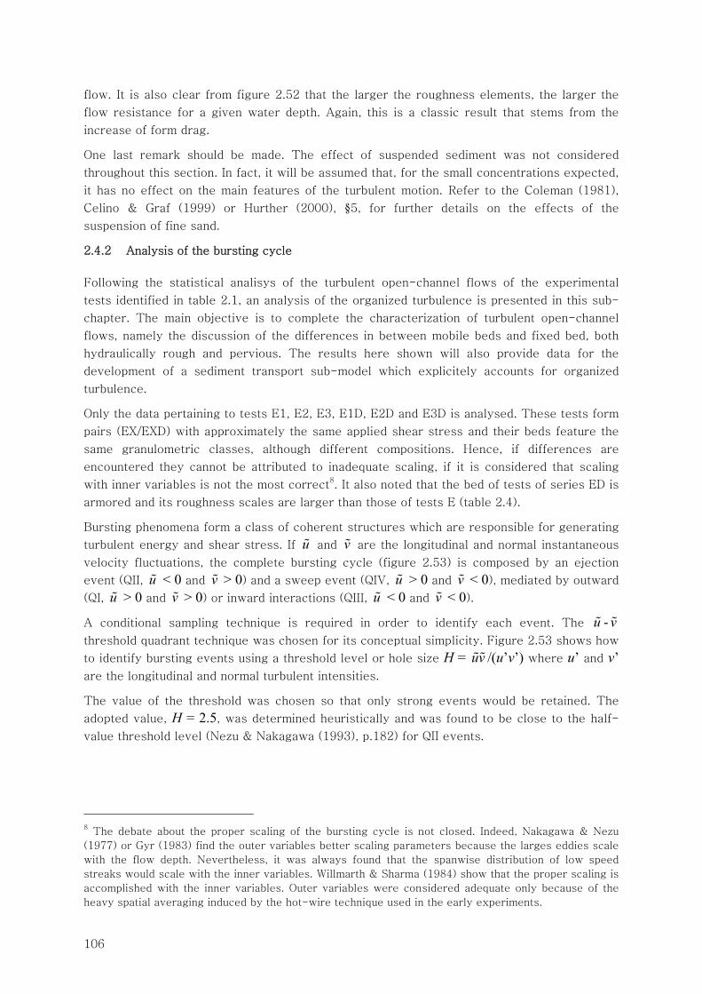
106

flow. It is also clear from figure 2.52 that the larger the roughness elements, the larger the

flow resistance for a given water depth. Again, this is a classic result that stems from the

increase of form drag.

One last remark should be made. The effect of suspended sediment was not considered

throughout this section. In fact, it will be assumed that, for the small concentrations expected,

it has no effect on the main features of the turbulent motion. Refer to the Coleman (1981),

Celino & Graf (1999) or Hurther (2000), §5, for further details on the effects of the

suspension of fine sand.

2.4.2 Analysis of the bursting cycle

Following the statistical analisys of the turbulent open-channel flows of the experimental

tests identified in table 2.1, an analysis of the organized turbulence is presented in this sub-

chapter. The main objective is to complete the characterization of turbulent open-channel

flows, namely the discussion of the differences in between mobile beds and fixed bed, both

hydraulically rough and pervious. The results here shown will also provide data for the

development of a sediment transport sub-model which explicitely accounts for organized

turbulence.

Only the data pertaining to tests E1, E2, E3, E1D, E2D and E3D is analysed. These tests form

pairs (EX/EXD) with approximately the same applied shear stress and their beds feature the

same granulometric classes, although different compositions. Hence, if differences are

encountered they cannot be attributed to inadequate scaling, if it is considered that scaling

with inner variables is not the most correct8. It also noted that the bed of tests of series ED is

armored and its roughness scales are larger than those of tests E (table 2.4).

Bursting phenomena form a class of coherent structures which are responsible for generating

turbulent energy and shear stress. If u and v are the longitudinal and normal instantaneous

velocity fluctuations, the complete bursting cycle (figure 2.53) is composed by an ejection

event (QII, u < 0 and v > 0) and a sweep event (QIV, u > 0 and v < 0), mediated by outward

(QI, u > 0 and v > 0) or inward interactions (QIII, u < 0 and v < 0).

A conditional sampling technique is required in order to identify each event. The u - v

threshold quadrant technique was chosen for its conceptual simplicity. Figure 2.53 shows how

to identify bursting events using a threshold level or hole size H = uv /(u’v’) where u’ and v’ are the longitudinal and normal turbulent intensities.

The value of the threshold was chosen so that only strong events would be retained. The

adopted value, H = 2.5, was determined heuristically and was found to be close to the half-

value threshold level (Nezu & Nakagawa (1993), p.182) for QII events.

8 The debate about the proper scaling of the bursting cycle is not closed. Indeed, Nakagawa & Nezu

(1977) or Gyr (1983) find the outer variables better scaling parameters because the larges eddies scale

with the flow depth. Nevertheless, it was always found that the spanwise distribution of low speed

streaks would scale with the inner variables. Willmarth & Sharma (1984) show that the proper scaling is

accomplished with the inner variables. Outer variables were considered adequate only because of the

heavy spatial averaging induced by the hot-wire technique used in the early experiments.

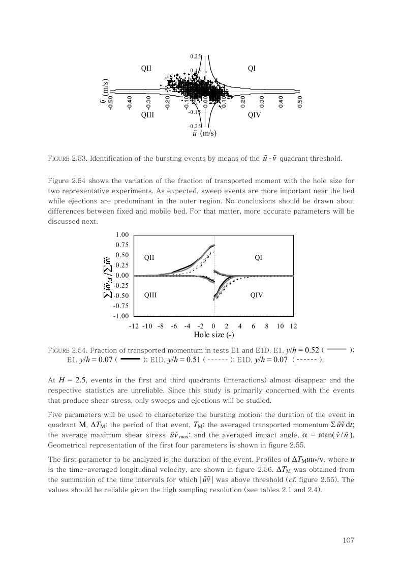
107

-0 .2 5

-0 .1 5

-0 .0 5

0 .0 5

0 .1 5

0 .2 5

u (m/s)

v (m

/s)

QII QI

QIII QIV

FIGURE 2.53. Identification of the bursting events by means of the u - v quadrant threshold.

Figure 2.54 shows the variation of the fraction of transported moment with the hole size for

two representative experiments. As expected, sweep events are more important near the bed

while ejections are predominant in the outer region. No conclusions should be drawn about

differences between fixed and mobile bed. For that matter, more accurate parameters will be

discussed next.

-1.00-0.75-0.50-0.250.000.250.500.751.00

-12 -10 -8 -6 -4 -2 0 2 4 6 8 10 12Hole size (-)

uvM/

uv

QII QI

QIII QIV

FIGURE 2.54. Fraction of transported momentum in tests E1 and E1D. E1, y/h = 0.52 ( );

E1, y/h = 0.07 ( ); E1D, y/h = 0.51 ( ); E1D, y/h = 0.07 ( ).

At H = 2.5, events in the first and third quadrants (interactions) almost disappear and the

respective statistics are unreliable. Since this study is primarily concerned with the events

that produce shear stress, only sweeps and ejections will be studied.

Five parameters will be used to characterize the bursting motion: the duration of the event in

quadrant M, ΔTM; the period of that event, TM; the averaged transported momentum Σuv dt; the average maximum shear stress uv max; and the averaged impact angle, α = atan( v /u ). Geometrical representation of the first four parameters is shown in figure 2.55.

The first parameter to be analyzed is the duration of the event. Profiles of ΔTMuu*/ν, where u

is the time-averaged longitudinal velocity, are shown in figure 2.56. ΔTM was obtained from

the summation of the time intervals for which |uv | was above threshold (cf. figure 2.55). The

values should be reliable given the high sampling resolution (see tables 2.1 and 2.4).

u

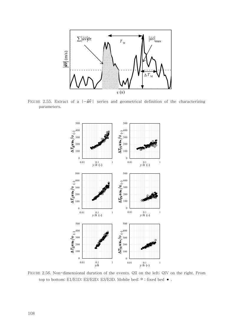
108

τ (s)

|uv

| (m

/s)

T M|uv |max

ΔT M

Σ|uv |dτ

FIGURE 2.55. Extract of a |–uv | series and geometrical definition of the characterizing

parameters.

0

100

200

300

400

500

0.01 0.1 1y /h (-)

ΔTIIU

u*/ ν

(-)

0

100

200

300

400

500

0.01 0.1 1y /h (-)

ΔΤIV

Uu

*/ ν (-

)

0

100

200

300

400

500

0.01 0.1 1y /h (-)

ΔTIIU

u*/ ν

(-)

0

100

200

300

400

500

0.01 0.1 1y /h (-)

ΔTIV

Uu

*/ ν (-

)

0

100

200

300

400

500

0.01 0.1 1y/h

ΔTIIU

u*/ ν

(-)

0

100

200

300

400

500

0.01 0.1 1y /h (-)

ΔTIV

Uu

*/ ν (-

)

FIGURE 2.56. Non-dimensional duration of the events. QII on the left; QIV on the right. From

top to bottom: E1/E1D; E2/E2D; E3/E3D. Mobile bed: ë ; fixed bed • .

duv τ∑ maxuv

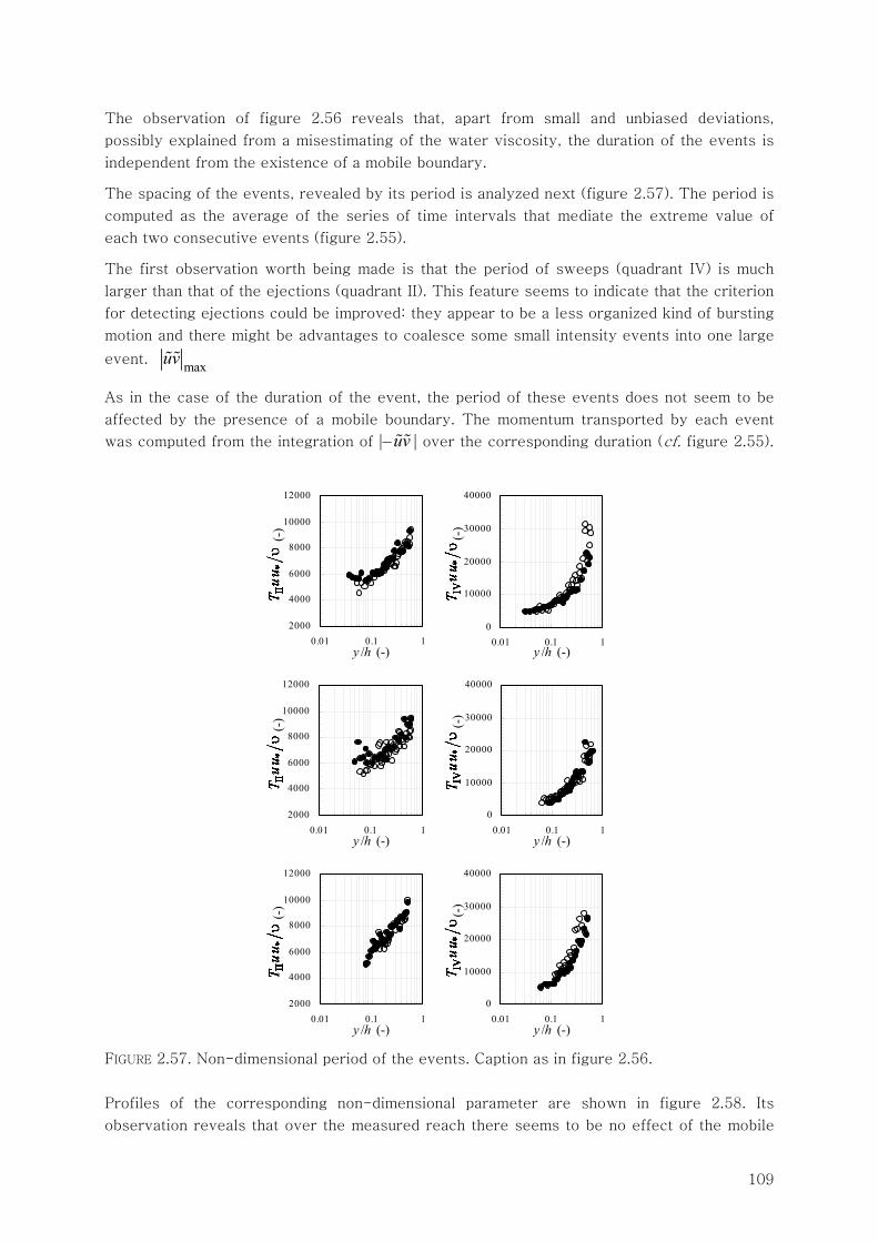
109

The observation of figure 2.56 reveals that, apart from small and unbiased deviations,

possibly explained from a misestimating of the water viscosity, the duration of the events is

independent from the existence of a mobile boundary.

The spacing of the events, revealed by its period is analyzed next (figure 2.57). The period is

computed as the average of the series of time intervals that mediate the extreme value of

each two consecutive events (figure 2.55).

The first observation worth being made is that the period of sweeps (quadrant IV) is much

larger than that of the ejections (quadrant II). This feature seems to indicate that the criterion

for detecting ejections could be improved: they appear to be a less organized kind of bursting

motion and there might be advantages to coalesce some small intensity events into one large

event. maxuv

As in the case of the duration of the event, the period of these events does not seem to be

affected by the presence of a mobile boundary. The momentum transported by each event

was computed from the integration of |–uv | over the corresponding duration (cf. figure 2.55).

2000

4000

6000

8000

10000

12000

0.01 0.1 1y /h (-)

TIIU

u */ ν

(-)

0

10000

20000

30000

40000

0.01 0.1 1y /h (-)

TIV

Uu

*/ ν (-

)

2000

4000

6000

8000

10000

12000

0.01 0.1 1y /h (-)

TIIU

u*/ ν

(-)

0

10000

20000

30000

40000

0.01 0.1 1y /h (-)

TIV

Uu *

/ ν (-

)

2000

4000

6000

8000

10000

12000

0.01 0.1 1y /h (-)

TIIU

u*/ ν

(-)

0

10000

20000

30000

40000

0.01 0.1 1y /h (-)

TIV

Uu

*/ ν (-

)

FIGURE 2.57. Non-dimensional period of the events. Caption as in figure 2.56.

Profiles of the corresponding non-dimensional parameter are shown in figure 2.58. Its

observation reveals that over the measured reach there seems to be no effect of the mobile

110

bed on the transported momentum. However, small changes may pass unnoticed due to data

scattering. For this reason, the ratio Σuv IV/Σuv II will be analyzed with more detail.

Figure 2.59 shows the vertical distribution of the average maximum value of |–uv |, here

called uv max, during an event (figure 2.55).A fundamental difference between mobile and

fixed beds is revealed: in the wall region the profiles clearly depart, revealing that the

maximum magnitude of the event is increased by the presence of a mobile bed. In the outer

region the results collapse visibly into a single curve.

Analyzing this feature with the previous ones, it can be said that the presence of the mobile

bed imposes a reorganization of the events. They become “sharper” albeit keeping the same

duration at the chosen threshold level. Further investigations on the variation of this

parameter with H should be carried out. Under the hypothesis that the transported momentum

does not vary significantly, changes on the shape of the uv series must produce effects on

higher order moments, namely the skewness and kurtosis.

5

10

15

20

25

0.01 0.1 1y /h (-)

Σuv

/(u*2 ) (

-)

5

10

15

20

25

0.01 0.1 1y /h (-)

Σuv

/(u*2 ) (

-)

5

10

15

20

25

0.01 0.1 1y /h (-)

Σuv

/(u*2 ) (

-)

5

10

15

20

25

0.01 0.1 1y /h (-)

Σuv

/(u*2 ) (

-)

5

10

15

20

25

0.01 0.1 1y /h (-)

Σuv

/(u*2 ) (

-)

5

10

15

20

25

0.01 0.1 1y /h (-)

Σuv

/(u*2 ) (

-)

FIGURE 2.58. Non-dimensional transported momentum. Caption as in figure 2.56.

It is interesting to notice that the profiles of the non-dimensional uv max seem to follow

a logarithmic law in the outer region modified with a damping function in the wall region:

max12

*ln ( / )

uv ya b y hhu

⎡ ⎤⎛ ⎞= − ϕ⎜ ⎟⎢ ⎥⎝ ⎠⎣ ⎦ (2.161)

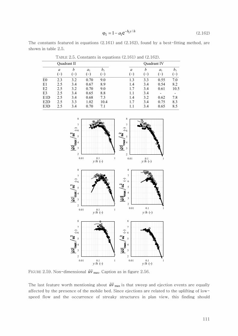
111

1 /1 11 e b y ha −ϕ = − (2.162)

The constants featured in equations (2.161) and (2.162), found by a best-fitting method, are

shown in table 2.5.

TABLE 2.5. Constants in equations (2.161) and (2.162). _____________________________________________________________________ Quadrant II Quadrant IV _________________________________ _________________________

a b a1 b1 a b a1 b1 (−) (−) (−) (−) (−) (−) (−) (−) ____________________________________________________________________

E0 2.3 3.2 0.70 9.0 1.3 3.3 0.55 7.0 E1 2.5 3.4 0.67 8.9 1.4 3.4 0.54 8.2 E2 2.5 3.2 0.70 9.0 1.7 3.4 0.61 10.5 E3 2.5 3.4 0.65 8.8 1.1 3.4 - - E1D 2.5 3.4 0.68 7.3 1.4 3.2 0.62 7.8 E2D 2.5 3.3 1.02 10.4 1.7 3.4 0.75 8.3 E3D 2.5 3.4 0.70 7.1 1.1 3.4 0.65 8.5 ____________________________________________________________________

2

3

4

5

6

7

8

0.01 0.1 1y /h (-)

uvm

ax/u

*2 (-)

2

3

4

5

6

7

8

0.01 0.1 1y /h (-)

uvm

ax/u

*2 (-)

2

3

4

5

6

7

8

0.01 0.1 1y /h (-)

uvm

ax/u

*2 (-)

2

3

4

5

6

7

8

0.01 0.1 1

y /h (-)

uvm

ax/u

*2 (-)

2

3

4

5

6

7

8

0.01 0.1 1y /h (-)

uvm

ax/u

*2 (-)

2

3

4

5

6

7

8

0.01 0.1 1y /h (-)

uvm

ax/u

*2 (-)

FIGURE 2.59. Non-dimensional uv max. Caption as in figure 2.56.

The last feature worth mentioning about uv max is that sweep and ejection events are equally

affected by the presence of the mobile bed. Since ejections are related to the uplifting of low-

speed flow and the occurrence of streaky structures in plan view, this finding should

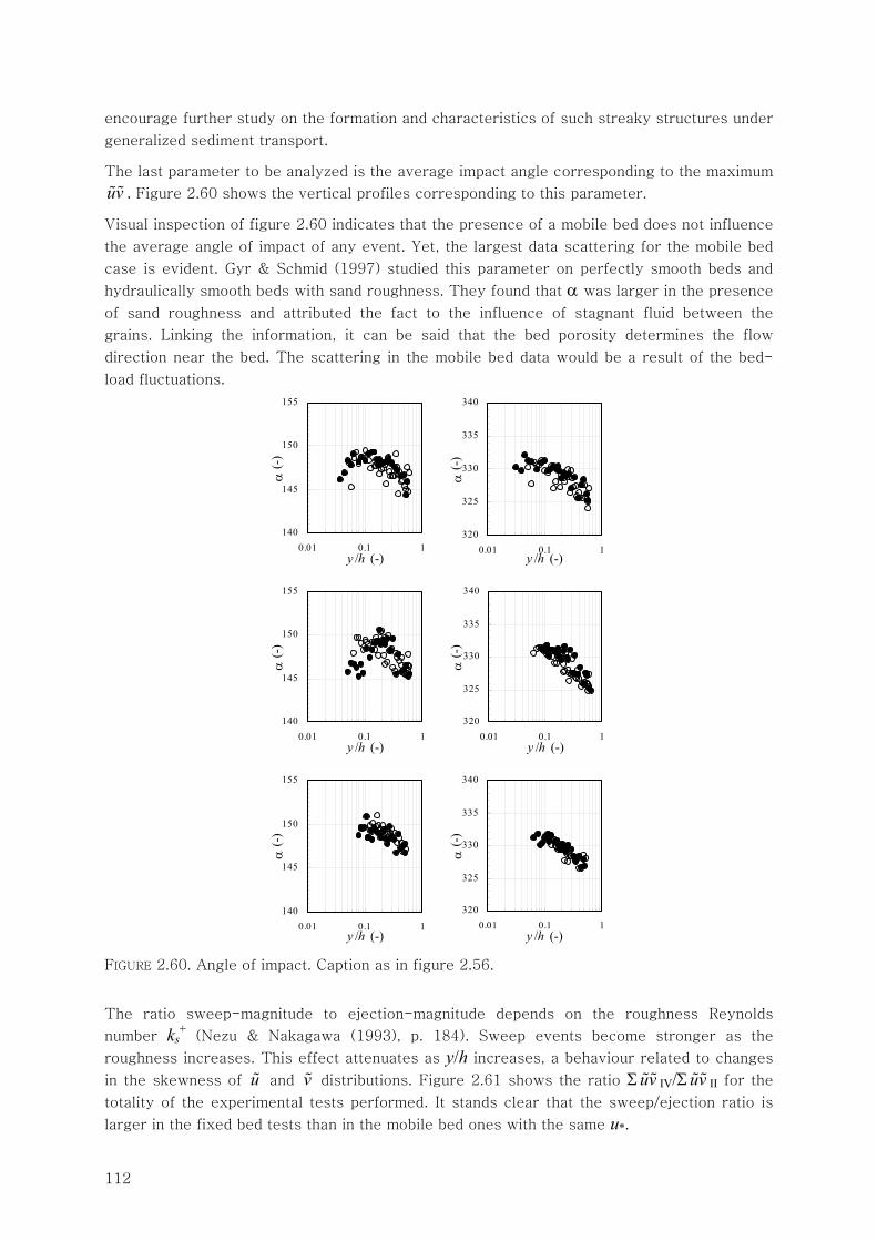
112

encourage further study on the formation and characteristics of such streaky structures under

generalized sediment transport.

The last parameter to be analyzed is the average impact angle corresponding to the maximum

uv . Figure 2.60 shows the vertical profiles corresponding to this parameter.

Visual inspection of figure 2.60 indicates that the presence of a mobile bed does not influence

the average angle of impact of any event. Yet, the largest data scattering for the mobile bed

case is evident. Gyr & Schmid (1997) studied this parameter on perfectly smooth beds and

hydraulically smooth beds with sand roughness. They found that α was larger in the presence

of sand roughness and attributed the fact to the influence of stagnant fluid between the

grains. Linking the information, it can be said that the bed porosity determines the flow

direction near the bed. The scattering in the mobile bed data would be a result of the bed-

load fluctuations.

140

145

150

155

0.01 0.1 1y /h (-)

α (-

)

320

325

330

335

340

0.01 0.1 1y /h (-)

α (-

)

140

145

150

155

0.01 0.1 1y /h (-)

α (-

)

320

325

330

335

340

0.01 0.1 1y /h (-)

α (-

)

140

145

150

155

0.01 0.1 1y /h (-)

α (-

)

320

325

330

335

340

0.01 0.1 1y /h (-)

α (-

)

FIGURE 2.60. Angle of impact. Caption as in figure 2.56.

The ratio sweep-magnitude to ejection-magnitude depends on the roughness Reynolds

number ks+ (Nezu & Nakagawa (1993), p. 184). Sweep events become stronger as the

roughness increases. This effect attenuates as y/h increases, a behaviour related to changes

in the skewness of u and v distributions. Figure 2.61 shows the ratio Σuv IV/Σuv II for the

totality of the experimental tests performed. It stands clear that the sweep/ejection ratio is

larger in the fixed bed tests than in the mobile bed ones with the same u*.

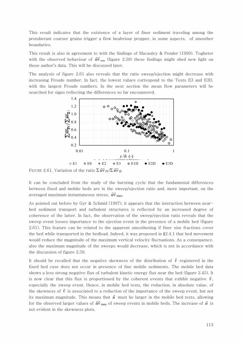
113

This result indicates that the existence of a layer of finer sediment traveling among the

protuberant coarser grains trigger a flow beahviour propper, in some aspects, of smoother

boundaries.

This result is also in agreement to with the findings of Macauley & Pender (1999). Togheter

with the observed behaviour of uv max (figure 2.59) these findings might shed new light on

those author’s data. This will be discussed later.

The analysis of figure 2.61 also reveals that the ratio sweep/ejection might decrease with

increasing Froude number. In fact, the lowest values correspond to the Tests E3 and E3D,

with the largest Froude numbers. In the next section the mean flow parameters will be

searched for signs reflecting the differences so far encountered.

0.2

0.4

0.6

0.8

1.0

1.2

1.4

0.01 0.1 1y /h (-)

uvIV

/uv

II

E1 E0 E2 E3 E1D E2D E3D

FIGURE 2.61. Variation of the ratio Σuv IV/Σuv II.

It can be concluded from the study of the bursting cycle that the fundamental differences

between fixed and mobile beds are in the sweep/ejection ratio and, more important, on the

averaged maximum instantaneous stress, uv max.

As pointed out before by Gyr & Schmid (1997), it appears that the interaction between near-

bed sediment transport and turbulent structures is reflected by an increased degree of

coherence of the latter. In fact, the observation of the sweep/ejection ratio reveals that the

sweep event looses importance to the ejection event in the presence of a mobile bed (figure

2.61). This feature can be related to the apparent smoothening if finer size fractions cover

the bed while transported in the bedload. Indeed, it was proposed in §2.4.1 that bed movement

would reduce the magnitude of the maximum vertical velocity fluctuations. As a consequence,

also the maximum magnitude of the sweeps would decrease, which is not in accordance with

the discussion of figure 2.59.

It should be recalled that the negative skewness of the distribution of v registered in the

fixed bed case does not occur in presence of fine mobile sediments. The mobile bed data

shows a less strong negative flux of turbulent kinetic energy flux near the bed (figure 2.45). It

is now clear that this flux is proportioned by the coherent events that exhibit negative v ,

especially the sweep event. Hence, in mobile bed tests, the reduction, in absolute value, of

the skewness of v is associated to a reduction of the importance of the sweep event, but not

its maximum magnitude. This means that u must be larger in the mobile bed tests, allowing

for the observed larger values of uv max of sweep events in mobile beds. The increase of u is

not evident in the skewness plots.

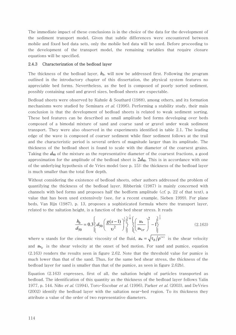
114

The immediate impact of these conclusions is in the choice of the data for the development of

the sediment transport model. Given that subtle differences were encountered between

mobile and fixed bed data sets, only the mobile bed data will be used. Before proceeding to

the development of the transport model, the remaining variables that require closure

equations will be specified.

2.4.3 Characterization of the bedload layer

The thickness of the bedload layer, hb, will now be addressed first. Following the program

outlined in the introductory chapter of this dissertation, the physical system features no

appreciable bed forms. Nevertheless, as the bed is composed of poorly sorted sediment,

possibly containing sand and gravel sizes, bedload sheets are expectable.

Bedload sheets were observed by Kuhnle & Southard (1988), among others, and its formation

mechanisms were studied by Seminara et al. (1996). Performing a stability study, their main

conclusion is that the development of bedload sheets is related to weak sediment sorting.

These bed features can be described as small amplitude bed forms developing over beds

composed of a bimodal mixture of sand and coarse sand or gravel under weak sediment

transport. They were also observed in the experiments identified in table 2.1. The leading

edge of the wave is composed of coarser sediment while finer sediment follows at the trail

and the characteristic period is several orders of magnitude larger than its amplitude. The

thickness of the bedload sheet is found to scale with the diameter of the coarsest grains.

Taking the d90 of the mixture as the representative diameter of the coarsest fractions, a good

approximation for the amplitude of the bedload sheet is 2d90. This is in accordance with one

of the underlying hypothesis of de Vries model (see p. 15): the thickness of the bedload layer

is much smaller than the total flow depth.

Without considering the existence of bedload sheets, other authors addressed the problem of

quantifying the thickness of the bedload layer. Ribberink (1987) is mainly concerned with

channels with bed forms and proposes half the bedform amplitude (cf. p. 22 of that text), a

value that has been used extensively (see, for a recent example, Sieben 1999). For plane

beds, Van Rijn (1987), p. 13, proposes a sophisticated formula where the transport layer,

related to the saltation height, is a function of the bed shear stress. It reads

171 2103

2*

50 250 *

( 1)0.3 1b

cr

h ug sdd u

⎧ ⎫⎧ ⎫ ⎛ ⎞−⎛ ⎞⎪ ⎪ ⎪ ⎪= −⎨ ⎬ ⎨ ⎬⎜ ⎟⎜ ⎟υ⎝ ⎠ ⎝ ⎠⎪ ⎪ ⎪ ⎪⎩ ⎭ ⎩ ⎭ (2.163)

where υ stands for the cinematic viscosity of the fluid, ( )

*w

bu = τ ρ is the shear velocity

and *cu is the shear velocity at the onset of bed motion. For sand and pumice, equation

(2.163) renders the results seen in figure 2.62. Note that the threshold value for pumice is

much lower than that of the sand. Thus, for the same bed shear stress, the thickness of the

bedload layer for sand is smaller than that of the pumice, as seen in figure 2.62b).

Equation (2.163) expresses, first of all, the saltation height of particles transported as

bedload. The identification of this quantity as the thickness of the bedload layer follows Yalin

1977, p. 144. Niño et al. (1994), Toro-Escobar et al. (1996), Parker et al. (2003), and DeVries

(2002) identify the bedload layer with the saltation near-bed region. To its thickness they

attribute a value of the order of two representative diameters.

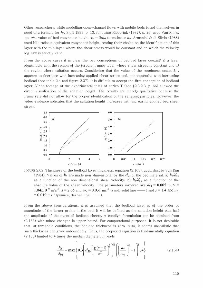
115

Other researchers, while modelling open-channel flows with mobile beds found themselves in

need of a formula for hb. Sloff 1993, p. 13, following Ribberink (1987), p. 26, uses Van Rijn’s,

op. cit., value of bed roughness height, ks = 3d90 to estimate hb. Armanini & di Silvio (1988)

used Nikuradse’s equivalent roughness height, resting their choice on the identification of this

layer with the thin layer where the shear stress would be constant and on which the velocity

log-law is strictly valid.

From the above cases it is clear the two conceptions of bedload layer coexist: i) a layer

identifiable with the region of the turbulent inner layer where shear stress is constant and ii)

the region where saltation occurs. Considering that the value of the roughness scale, ks+,

appears to decrease with increasing applied shear stress and, consequently, with increasing

bedload (see table 2.4 and figure 2.37), it is difficult to accept the first conception of bedload

layer. Video footage of the experimental tests of series T (see §2.3.2.3, p. 66) allowed the

direct visualisation of the saltation height. The results are merely qualitative because the

frame rate did not allow for the proper identification of the saltating particles. However, the

video evidence indicates that the saltation height increases with increasing applied bed shear

stress.

0.00.51.01.52.02.53.03.54.04.5

0 1 2 3 4 5u */u *cr (-)

h b/d

50

(-)

0.0

1.0

2.0

3.0

4.0

5.0

6.0

0 0.05 0.1 0.15 0.2 0.25u * (ms-1)

h b/d

50

(-)

FIGURE 2.62. Thickness of the bedload layer thickness, equation (2.163), according to Van Rijn

(1984). Values of hb are made non-dimensional by the d50 of the bed material. a) hb/d50

as a function of the non-dimensional shear velocity; b) hb/d50 as a function of the

absolute value of the shear velocity. The parameters involved are d50 = 0.005 m, ν = 1.04x10−6

m2s−1, s = 2.65 and u*c = 0.031 ms−1 (sand, solid line ) and s = 1.4 and u*c = 0.019 ms−1 (pumice, dashed line ).

From the above considerations, it is assumed that the bedload layer is of the order of

magnitude of the larger grains in the bed. It will be defined as the saltation height plus half

the amplitude of the eventual bedload sheets. A condign formulation can be obtained from

(2.163) with minor changes in upper bound. For computational purposes, it is not desirable

that, at threshold conditions, the bedload thickness is zero. Also, it seems unrealistic that

such thickness can grow unboundedly. Thus, the proposed equation is fundamentally equation

(2.163) limited to 4 times the median diameter. It reads

171 2103

2*

50 250 *

( 1)max 0.3 1 ,4b

c

h ug sdd u

⎧ ⎫⎛ ⎞⎛ ⎞ ⎛ ⎞−⎛ ⎞⎪ ⎪⎜ ⎟⎜ ⎟= −⎨ ⎬⎜ ⎟⎜ ⎟⎜ ⎟ ⎜ ⎟υ⎝ ⎠ ⎝ ⎠⎪ ⎪⎝ ⎠ ⎝ ⎠⎩ ⎭

(2.164)

a) b)

116

where * 0.029cu = ms-1.

The layer velocity, ub, requires i) the definition of the depth-averaged concentrations

corresponding to each sediment class, ii) the velocity of each class k, ucbk, and iii) the velocity

of the water in the bedload layer, uwb, (see equations (2.39) or (2.113)). The concentrations

will be determined in the next sub-chapters.

The values of the average velocity of the sediment, ucbk, were determined with the help of the

particle tracking algorithm described in Annex 2.4, p. 171. Figure 2.63 shows examples of

paths of particles detected by the algorithm. The paths show an apron-like shape, typical of

particles entrained by turbulent sweep events.

0

1

2

3

4

5

6

-2 -1 0 1 2

lateral direction (cm)

alon

g-st

ream

dire

ctio

n (c

m)

0

1

2

3

4

5

6

-2 -1 0 1 2

lateral direction (cm)

alon

g-st

eam

dire

ctio

n (c

m)

FIGURE 2.63. Results of the particle tracking algorithm. Each plot shows the path of the

particles affected by one mild sweep event in test T3. Circles represent successive

positions of the particles in each frame.

It is considered that the particle ceases to move when its displacement is less than half its

diameter. Thus, it is clear that these velocities do not correspond to the ballistic range, in the

terms of Nikora et al. (2002). Since they incorporate the slow ends of the histogram of

velocities, it is more appropriate to classify them as intermediate range velocities. This is the

appropriate range for the definition of the bedload. Indeed, as mentioned in §2.2.2.5, it is

likely that, at a given instant, all modes of transport are present crossing the imaginary line

that allows for defining the bedload discharge.

The average velocity of the sediment particles is computed as the ensemble average, over a

large number of particles, of the path-averaged velocity in the along-stream direction. The

results, for the size fractions characterized by d = 0.606, 0.925, 1.5, 2.4, 3.1, 4.0, 5.5 and 6.4

mm, are shown in figure 2.64. It is observable that the average velocity of each size fraction

follows a linear trend.

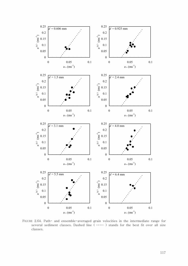
117

0

0.05

0.1

0.15

0.2

0.25

0 0.05 0.1u * (ms-1)

u(g

) (m

s-1)

d = 0.606 mm

0

0.05

0.1

0.15

0.2

0.25

0 0.05 0.1u * (ms-1)

u(g

) (m

s-1)

d = 0.925 mm

0

0.05

0.1

0.15

0.2

0.25

0 0.05 0.1u * (ms-1)

u(g

) (m

s-1)

d = 1.5 mm

0

0.05

0.1

0.15

0.2

0.25

0 0.05 0.1u * (ms-1)

u(g

) (m

s-1)

d = 2.4 mm

0

0.05

0.1

0.15

0.2

0.25

0 0.05 0.1u * (ms-1)

u(g

) (m

s-1)

d = 3.1 mm

0

0.05

0.1

0.15

0.2

0.25

0 0.05 0.1u * (ms-1)

u(g

) (m

s-1)

d = 4.0 mm

0

0.05

0.1

0.15

0.2

0.25

0 0.05 0.1u * (ms-1)

u(g

) (m

s-1)

d = 5.5 mm

0

0.05

0.1

0.15

0.2

0.25

0 0.05 0.1u * (ms-1)

u(g

) (m

s-1)

d = 6.4 mm

FIGURE 2.64. Path- and ensemble-averaged grain velocities in the intermediate range for

several sediment classes. Dashed line ( ) stands for the best fit over all size

classes.

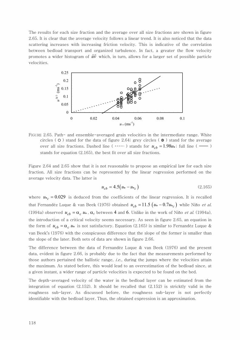
118

The results for each size fraction and the average over all size fractions are shown in figure

2.65. It is clear that the average velocity follows a linear trend. It is also noticed that the data

scattering increases with increasing friction velocity. This is indicative of the correlation

between bedload transport and organized turbulence. In fact, a greater the flow velocity

promotes a wider histogram of uv which, in turn, allows for a larger set of possible particle

velocities.

0

0.05

0.1

0.15

0.2

0.25

0 0.02 0.04 0.06 0.08 0.1u * (ms-1)

u(g

) (m

s-1)

FIGURE 2.65. Path- and ensemble-averaged grain velocities in the intermediate range. White

circles ( ) stand for the data of figure 2.64; grey circles ( ) stand for the average

over all size fractions. Dashed line ( ) stands for *1.98cbu u= ; full line ( )

stands for equation (2.165), the best fit over all size fractions.

Figure 2.64 and 2.65 show that it is not reasonable to propose an empirical law for each size

fraction. All size fractions can be represented by the linear regression performed on the

average velocity data. The latter is

( )* *4.5cb cu u u= − (2.165)

where * 0.029cu = is deduced from the coefficients of the linear regression. It is recalled

that Fernandéz Luque & van Beek (1976) obtained ( )* *11.5 0.7cb cu u u= − while Niño et al.

(1994a) observed *cb cu u= α , αc between 4 and 6. Unlike in the work of Niño et al. (1994a),

the introduction of a critical velocity seems necessary. As seen in figure 2.65, an equation in

the form of *cb cu u= α is not satisfactory. Equation (2.165) is similar to Fernandéz Luque &

van Beek’s (1976) with the conspicuous difference that the slope of the former is smaller than

the slope of the later. Both sets of data are shown in figure 2.66.

The difference between the data of Fernandéz Luque & van Beek (1976) and the present

data, evident in figure 2.66, is probably due to the fact that the measurements performed by

those authors pertained the ballistic range, i.e., during the jumps where the velocities attain

the maximum. As stated before, this would lead to an overestimation of the bedload since, at

a given instant, a wider range of particle velocities is expected to be found on the bed.

The depth-averaged velocity of the water in the bedload layer can be estimated from the

integration of equation (2.152). It should be recalled that (2.152) is stricktly valid in the

roughness sub-layer. As discussed before, the roughness sub-layer is not perfectly

identifiable with the bedload layer. Thus, the obtained expression is an approximation.

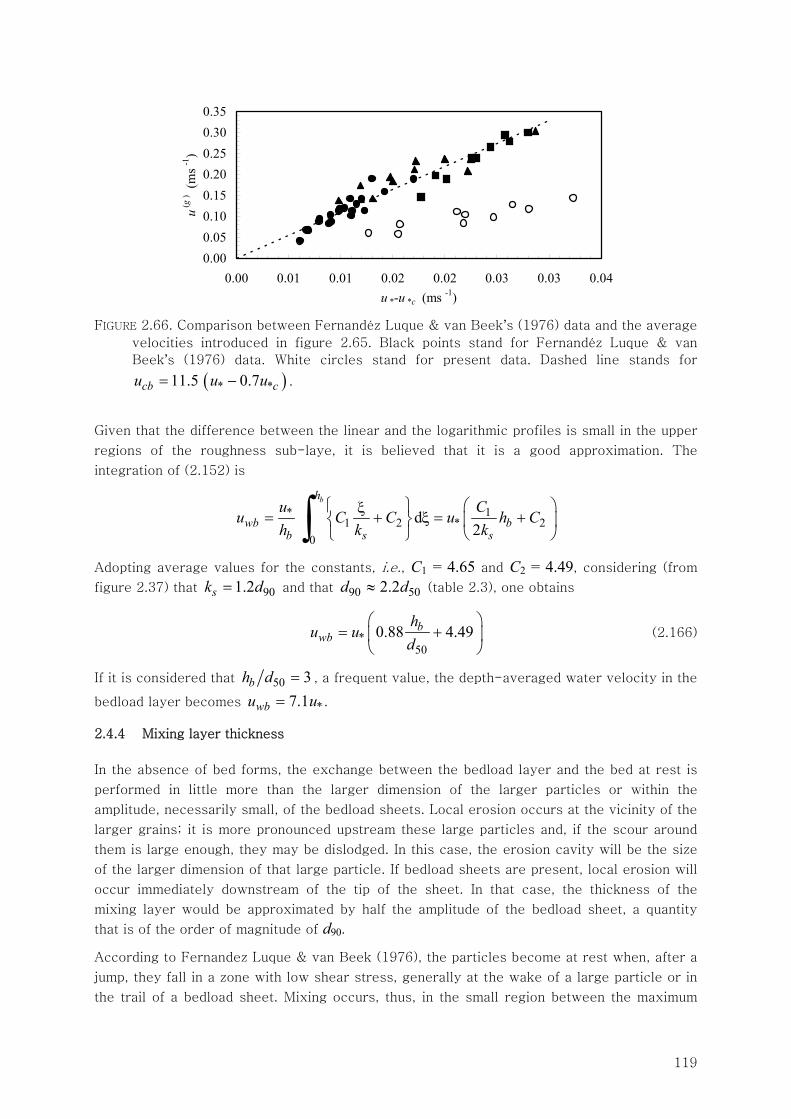
119

0.000.050.100.150.200.250.300.35

0.00 0.01 0.01 0.02 0.02 0.03 0.03 0.04u *-u *c (ms -1)

u(g

) (m

s -1)

FIGURE 2.66. Comparison between Fernandéz Luque & van Beek’s (1976) data and the average

velocities introduced in figure 2.65. Black points stand for Fernandéz Luque & van

Beek’s (1976) data. White circles stand for present data. Dashed line stands for

( )* *11.5 0.7cb cu u u= − .

Given that the difference between the linear and the logarithmic profiles is small in the upper

regions of the roughness sub-laye, it is believed that it is a good approximation. The

integration of (2.152) is

* 11 2 * 2

0

d2

bh

wb bb s s

u Cu C C u h Ch k k

⎧ ⎫ ⎛ ⎞ξ= + ξ = +⎨ ⎬ ⎜ ⎟

⎩ ⎭ ⎝ ⎠∫

Adopting average values for the constants, i.e., C1 = 4.65 and C2 = 4.49, considering (from

figure 2.37) that 901.2sk d= and that 90 502.2d d≈ (table 2.3), one obtains

*50

0.88 4.49bwb

hu u

d⎛ ⎞

= +⎜ ⎟⎝ ⎠

(2.166)

If it is considered that 50 3bh d = , a frequent value, the depth-averaged water velocity in the

bedload layer becomes *7.1wbu u= .

2.4.4 Mixing layer thickness

In the absence of bed forms, the exchange between the bedload layer and the bed at rest is

performed in little more than the larger dimension of the larger particles or within the

amplitude, necessarily small, of the bedload sheets. Local erosion occurs at the vicinity of the

larger grains; it is more pronounced upstream these large particles and, if the scour around

them is large enough, they may be dislodged. In this case, the erosion cavity will be the size

of the larger dimension of that large particle. If bedload sheets are present, local erosion will

occur immediately downstream of the tip of the sheet. In that case, the thickness of the

mixing layer would be approximated by half the amplitude of the bedload sheet, a quantity

that is of the order of magnitude of d90.

According to Fernandez Luque & van Beek (1976), the particles become at rest when, after a

jump, they fall in a zone with low shear stress, generally at the wake of a large particle or in

the trail of a bedload sheet. Mixing occurs, thus, in the small region between the maximum

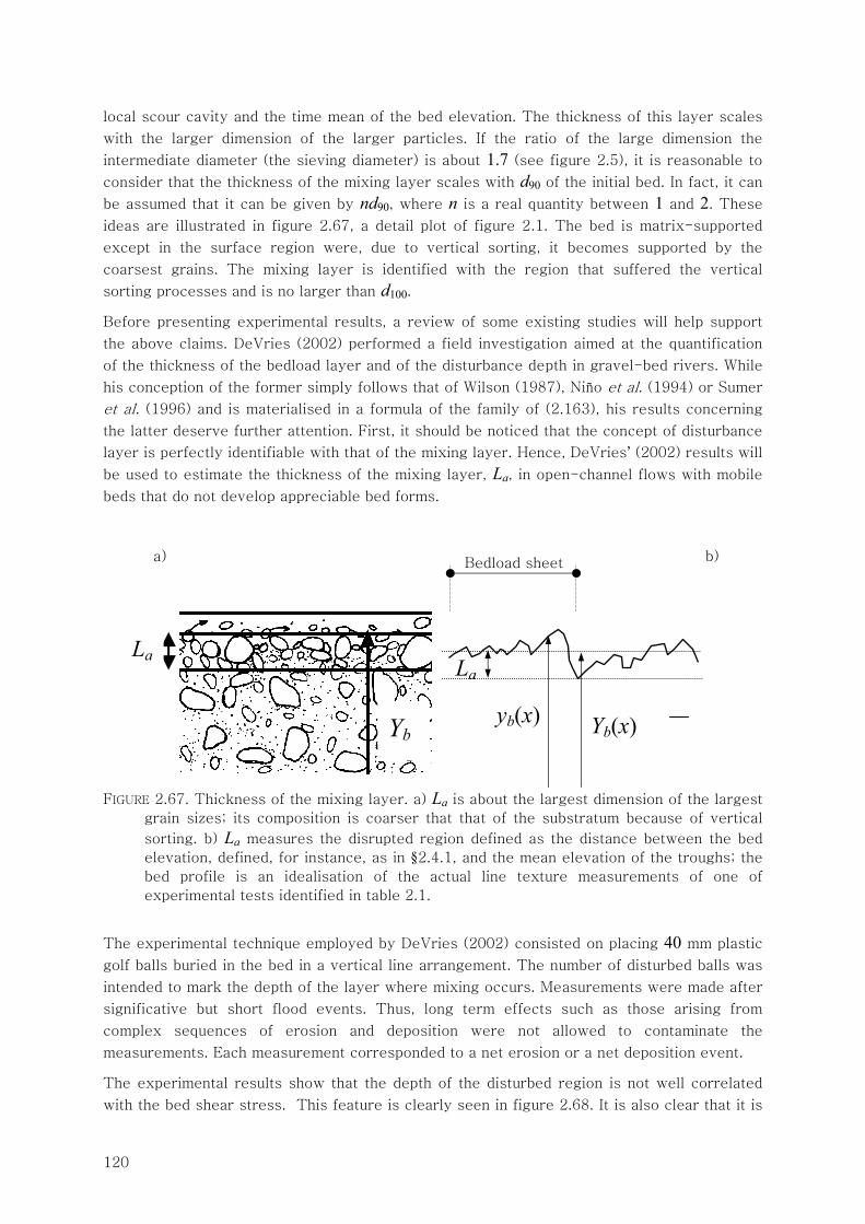
120

local scour cavity and the time mean of the bed elevation. The thickness of this layer scales

with the larger dimension of the larger particles. If the ratio of the large dimension the

intermediate diameter (the sieving diameter) is about 1.7 (see figure 2.5), it is reasonable to

consider that the thickness of the mixing layer scales with d90 of the initial bed. In fact, it can

be assumed that it can be given by nd90, where n is a real quantity between 1 and 2. These

ideas are illustrated in figure 2.67, a detail plot of figure 2.1. The bed is matrix-supported

except in the surface region were, due to vertical sorting, it becomes supported by the

coarsest grains. The mixing layer is identified with the region that suffered the vertical

sorting processes and is no larger than d100.

Before presenting experimental results, a review of some existing studies will help support

the above claims. DeVries (2002) performed a field investigation aimed at the quantification

of the thickness of the bedload layer and of the disturbance depth in gravel-bed rivers. While

his conception of the former simply follows that of Wilson (1987), Niño et al. (1994) or Sumer

et al. (1996) and is materialised in a formula of the family of (2.163), his results concerning

the latter deserve further attention. First, it should be noticed that the concept of disturbance

layer is perfectly identifiable with that of the mixing layer. Hence, DeVries’ (2002) results will

be used to estimate the thickness of the mixing layer, La, in open-channel flows with mobile

beds that do not develop appreciable bed forms.

FIGURE 2.67. Thickness of the mixing layer. a) La is about the largest dimension of the largest

grain sizes; its composition is coarser that that of the substratum because of vertical

sorting. b) La measures the disrupted region defined as the distance between the bed

elevation, defined, for instance, as in §2.4.1, and the mean elevation of the troughs; the

bed profile is an idealisation of the actual line texture measurements of one of

experimental tests identified in table 2.1.

The experimental technique employed by DeVries (2002) consisted on placing 40 mm plastic

golf balls buried in the bed in a vertical line arrangement. The number of disturbed balls was

intended to mark the depth of the layer where mixing occurs. Measurements were made after

significative but short flood events. Thus, long term effects such as those arising from

complex sequences of erosion and deposition were not allowed to contaminate the

measurements. Each measurement corresponded to a net erosion or a net deposition event.

The experimental results show that the depth of the disturbed region is not well correlated

with the bed shear stress. This feature is clearly seen in figure 2.68. It is also clear that it is

Yb

La

Bedload sheet

yb(x) Yb(x)

La

a) b)

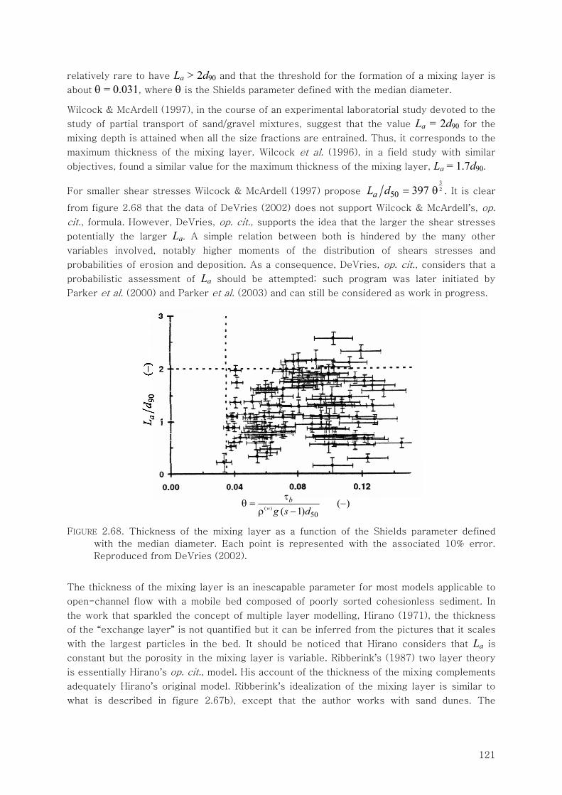
121

relatively rare to have La > 2d90 and that the threshold for the formation of a mixing layer is

about θ = 0.031, where θ is the Shields parameter defined with the median diameter.

Wilcock & McArdell (1997), in the course of an experimental laboratorial study devoted to the

study of partial transport of sand/gravel mixtures, suggest that the value La = 2d90 for the

mixing depth is attained when all the size fractions are entrained. Thus, it corresponds to the

maximum thickness of the mixing layer. Wilcock et al. (1996), in a field study with similar

objectives, found a similar value for the maximum thickness of the mixing layer, La = 1.7d90.

For smaller shear stresses Wilcock & McArdell (1997) propose 32

50 397aL d = θ . It is clear

from figure 2.68 that the data of DeVries (2002) does not support Wilcock & McArdell’s, op.

cit., formula. However, DeVries, op. cit., supports the idea that the larger the shear stresses

potentially the larger La. A simple relation between both is hindered by the many other

variables involved, notably higher moments of the distribution of shears stresses and

probabilities of erosion and deposition. As a consequence, DeVries, op. cit., considers that a

probabilistic assessment of La should be attempted; such program was later initiated by

Parker et al. (2000) and Parker et al. (2003) and can still be considered as work in progress.

FIGURE 2.68. Thickness of the mixing layer as a function of the Shields parameter defined

with the median diameter. Each point is represented with the associated 10% error.

Reproduced from DeVries (2002).

The thickness of the mixing layer is an inescapable parameter for most models applicable to

open-channel flow with a mobile bed composed of poorly sorted cohesionless sediment. In

the work that sparkled the concept of multiple layer modelling, Hirano (1971), the thickness

of the “exchange layer” is not quantified but it can be inferred from the pictures that it scales

with the largest particles in the bed. It should be noticed that Hirano considers that La is

constant but the porosity in the mixing layer is variable. Ribberink’s (1987) two layer theory

is essentially Hirano’s op. cit., model. His account of the thickness of the mixing complements

adequately Hirano’s original model. Ribberink’s idealization of the mixing layer is similar to

what is described in figure 2.67b), except that the author works with sand dunes. The

( )50

( )( 1)w

bg s d

τθ = −

ρ −

122

average procedure for the trough elevation involves the use of weighting coefficients that

describe the probability of deposition of a given size fraction.

Belleudy (2000) and (2001) uses “the size of the largest grain”, a formulation that echoes the

experimental advances cited above. Sieben (1999) propose that La = dm, where dm is the mean

diameter in the mixing layer. A similar proposal, La = d84 of the mixing layer, is made by Hoey

& Ferguson (1994). These authors warn that their computational solution becomes

“necessarily iterative” because the mass of the mixing layer, depending on its volume and

hence on its thickness, is a function of its composition. As seen in Chapter 5 (see §5.5), the

solution is not necessarily iterative, in absolute sense, but having La depending on a diameter

of the mixing layer does pose serious stability challenges. Unimpressed by this difficulty,

Toro-Escobar et al. (1996), following Parker (1990), use a quite similar formula, La = d90,

where the d90 is that of the mixing layer. On the contrary, Vogel et al. (1992), aware of the

computational difficulties, propose a constant value for the thickness La. It is determined by

50502a b critL d= τ τ where the critical shear stress is that of the d50. Both shear stresses are

computed prior to the simulation.

Earlier modelling attempts by Holly & Rahuel (1990) and Rahuel et al. (1989), following

Kennedy’s (1963) dune studies, use half the dune height. Algebraically this is materialized in

La = εh, [ ]0.1,0.2ε ∈ . Armanini & di Silvio (1988) propose La = hb but add the computational

restriction that La should not be smaller that 0.05h.

Armanini (1995) claimed that the equation of conservation of the sediment mass in the mixing

layer, as presented by Hirano (1971), can be sought as vertical first order space

discretization of a diffusive equation for which the vertical mesh size is of the order of the

largest grains in the bed. Decomposing the bed elevation, the sediment discharge and other

sediment related variables into a mean and a fluctuating part, Armanini, op. cit., shows that

sediment mixing can be expressed as a diffusive process. The corresponding second order

PDF can be solved with boundary conditions at the bed surface and at infinite depth that

describe the bedload composition (at the surface) and the undisturbed bed composition (at

large depths).

It is a fundamental premise of this view that the sediment distribution in the mixing layer is

not uniform but variable in depth. It is a continuous curve connecting the bedload composition

to the composition of the undisturbed bed, at great depths. Recent experimental data, partially

published in Sibanda et al. (2000), would help explain whether there is a region where mixing

is complete and the sediment distribution is uniform or if the bed composition changes

continuously across the mixing layer. This research line is open and appears promising.

In the present text, given the lack of appreciable bed forms, the thickness of the mixing layer

will be taken to be

902aL d= (2.167)

The thickness of the layer is important as it controls the time for which armouring occurs by

controlling the volume of exposed fine sediment. Thus, a good estimate is necessary. The

small variations that d90 might incur over the time are negligible for this purpose but pose

considerable numerical risks. The interdependence between La and bed composition causes

123

feedback problems that lead to instability even if hyperbolic stability is assured. Thus, the

diameter corresponding to percentile 90 in (2.167) should be that of the initial bed.

2.4.5 Shear stresses and sediment concentrations

As stated before, it is assumed that the sediment can be transported in suspension or as

contact load. In the bedload layer, the coarse particles are transported as contact load but

there might be finer particles carried in suspension. Thus, to identify bedload – the sediment

load carried in the region adjacent to the bed – with contact load is a simplification. On the

contrary, in the suspended sediment layer there are only fine particles carried in suspension.

The distinction between contact load and suspended sediment is based on the effects of

hydrodynamic lift and drag forces upon the particles. Ever since Kalinske 1947 (see

Fernandez Luque & van Beek 1976), Mayer-Peter & Müller, 1948 (see Yalin 1977, pp. 113-

117) and Einstein (1950), it has been observed that the fluid flow transfers momentum to the

sediment particles on the bed surface. This action is materialised on drag and lift forces.

According to Einstein (1950), the particle, after being acted upon, describes a perfect

parabolic trajectory, which indicates that lift forces are not important. Fernandez Luque & van

Beek (1976) and more recently Niño & Garcia (1996) challenged this view. Their

experimental data, mostly recorded particle paths, show that saltating particles have

elongated trajectories and, hence, do suffer some lift.

If the particles move in relatively small jumps (e.g., 10 – 20 diameters as observed by Drake

et al. 1988) and fall back to the bed, the time average of the vertical component of reaction

force at the bed is close to the submerged weight of the moving material. This fact prompted

Bagnold (1966) to devise a transport formula based on the premise that the fluid flow acts as

a “transport machine” with a given efficiency that would spend work transporting material

moving near the bed. To define this work he used a longitudinal force computed from the

weigh of the particles in movement times a coefficient of dynamic friction. The term contact

load (see Wilson 1987) becomes, thus, synonym of a mode of transport where the

hydrodynamic actions upon a particle undergoing a jump do not involve lift and the vertical

actions are reaction forces aroused in the frequent collisions at the bed9. Contact load differs

from bedload inasmuch the latter is described by formulas that do not involve explicitly the

flow depth, h (definition in Yalin 1977, p. 112). Thus, bedload occurs necessarily in a small,

sometimes negligible, portion of the total depth, which is not true in the case of the contact

load (see Chapter 3, §3.7.2).

The concentrations associated to contact load range from zero, at the onset of motion, to

about 0.5 for heavy-laden sheet flows (Wilson 1987). In this chapter, attention is devoted to

size selective sediment transport. The largest size fractions in the bed are expected to

display reduced mobility as its critical shear stress is less or about the mean applied shear

stress. Expected concentrations of coarse particles in the bedload layer are in the range of

0.0 to 0.1. For instance, a given flow with a depth of 0.6 m and a gravel distribution with a

mean diameter of 3 mm, a concentration larger than 1x10−1 would require a Froude number

9 It should be made clear that bedload formulas of Einstein (1950) and Bagnold (1966) are of very

different nature. The former is based on the average jump length and on the probabilities of entrainment

and distrainment. The latter is derived, as explained, from the work spent by the flow to displace a

given mass of particles. Both require the contact load assumption, though.

124

larger than 0.7, which is seldom found in gravel rivers. These calculi were performed with

Bagnold’s (1956) formula.

The research conducted by Paintal 1969 was probably the first in which video analysis was

used to quantify the motion of gravel (cf. Drake et al. 1988). It was followed by Fernandez

Luque & van Beek (1976), Sumer & Deigaard (1981), Drake et al. (1988), Nelson et al.

(1995), Niño et al. (1994), Niño & Garcia (1994), Sechet & LeGuennec (1999) and Nikora et

al. (2002) to name only a few, considered more significative. The span of possible bed motion

types is rather wide. Drake et al. (1988), for instance, categorizes the motion into rolling,

sliding, saltation. All of these types of motion can be considered contact load. If the jump of

the particle becomes too long and its contacts with the bed become more sporadic, the

particle is at the onset of suspension (Gyr 1983, Niño et al. 2003). Eventually the fluid would

provide the upward force to support the particle without any interaction with the bed. In that

case, the particle is said to be in suspension,

An overview of the recent suspended sediment models reveals that i) turbulent motion must

be at the root of the entrainment and suspension mechanisms (Cellino & Graf 1999) ii)

coherent turbulent structures such as ejections (second quadrant) or outward interactions

(first quadrant) are responsible for most entrainment episodes (Nezu & Nakagawa 1993,

§12.2, Hurther 2002, p. 145) and iii) turbulent intensities are likely to be affected by the

presence of suspended sediment (drag reduction, Wei & Wilmarth 1992).

The concentrations of suspended sediment are expected to be very low. In this case, the

turbulent stresses in the suspended sediment layer are not dramatically distinct from those

corresponding to clear water. As for the turbulent stresses in the bedload layer, the presence

of coarse sediment in motion will necessarily affect the momentum balance, as the sediment

particles drain momentum from the fluid flow. In a uniform flow under capacity (or

equilibrium) sediment transport, the momentum balance in the longitudinal direction is

( ) ( )( ) (2) ( )ˆd 1 sin( ) 0w gwy f g C Fτ + ρ − β + = (2.168)

( ) ( ) (2) ( )ˆd sin( ) 0w gwy s sC g Fτ + ρ β − = (2.169)

respectively for the fluid flow and for sediment grains. In these equations β is the angle

between the bed and a horizontal plane, (2) (2)( )C C y= is the concentration at a given

elevation above the bed and ( )gwF is the drag force, per unit volume, exerted on the sediment

particles. These equations admit the following boundary conditions: ( 0)f fbyτ = = τ ,

( )(2)ˆ( ) sin( )f b by h g h hτ = = ρ − β , ( 0)s sbyτ = = τ and ( ) 0s by hτ = = . It is clear from

equations (2.168) and (2.169) that the fluid shear stress must diminish from its value at the

upper boundary to a minimum at the bed, as seen in figure 2.69. Conversely, the shear stress

associated with the solid particles increases. Obviously, the drag force, function of the

relative velocity is responsible for this behaviour.

Stresses at the bed can be computed from the integration of equations (2.168) and (2.169).

The integration process renders

( ) (2) ( )

00 0

sin( ) (1 )d d 0b b

w gw

b

h h

f fy h yg C y F y

= =τ − τ + ρ β − − =∫ ∫

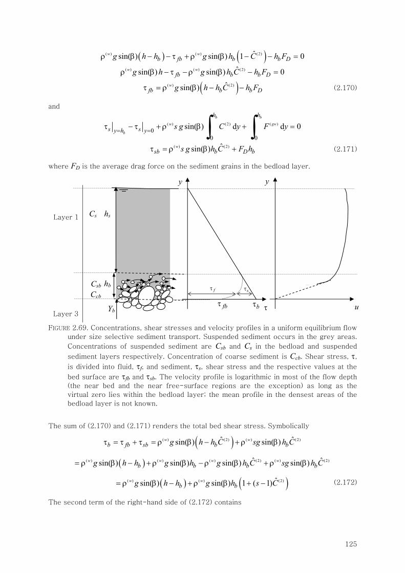
125

( ) ( )( ) ( ) (2)ˆsin( ) sin( ) 1 0w wb fb b b Dg h h g h C h Fρ β − − τ + ρ β − − =

( ) ( ) (2)ˆsin( ) sin( ) 0w w

fb b b Dg h g h C h Fρ β − τ − ρ β − =

( )( ) (2)ˆsin( )wfb b b Dg h h C h Fτ = ρ β − − (2.170)

and

( ) (2) ( )

00 0

sin( ) d d 0b b

w gw

b

h h

s sy h y s g C y F y= =τ − τ + ρ β + =∫ ∫

( ) (2)ˆsin( )w

sb b D bs g h C F hτ = ρ β + (2.171)

where FD is the average drag force on the sediment grains in the bedload layer.

FIGURE 2.69. Concentrations, shear stresses and velocity profiles in a uniform equilibrium flow

under size selective sediment transport. Suspended sediment occurs in the grey areas.

Concentrations of suspended sediment are Csb and Cs in the bedload and suspended

sediment layers respectively. Concentration of coarse sediment is Ccb. Shear stress, τ,

is divided into fluid, τf, and sediment, τs, shear stress and the respective values at the

bed surface are τfb and τsb. The velocity profile is logarithmic in most of the flow depth

(the near bed and the near free-surface regions are the exception) as long as the

virtual zero lies within the bedload layer; the mean profile in the densest areas of the

bedload layer is not known.

The sum of (2.170) and (2.171) renders the total bed shear stress. Symbolically

( )( )

( ) ( )

( ) (2) ( ) (2)

( ) ( ) ( ) (2) ( ) (2)

( ) ( ) (2)

ˆ ˆsin( ) sin( )

ˆ ˆsin( ) sin( ) sin( ) sin( )

ˆsin( ) sin( ) 1 ( 1)

w w

w w w w

w w

b fb sb b b

b b b b

b b

g h h C sg h C

g h h g h g h C sg h C

g h h g h s C

τ = τ + τ = ρ β − + ρ β

= ρ β − + ρ β − ρ β + ρ β

= ρ β − + ρ β + −

(2.172)

The second term of the right-hand side of (2.172) contains

hs

hb

Yb

Layer 1 Cs

Layer 3 τfbτ

y y

ubτ

fτ sτCcb Csb

126

( )(2) ( ) (2)ˆˆ 1 ( 1)w s Cρ = ρ + − (2.173)

which is the depth-averaged density of the mixture in the bedload layer. In uniform flow and

equilibrium sediment transport conditions, the thickness of the bedload layer can be

expressed by

(2)

( )

ˆ sin( )( 1)w

b sh dm m

h h sρ β

= θ =ρ −

(2.174)

where m is a constant which, from equation (2.164), is O(1) to O(10) . It follows that

( ) ( )O sin( ) <O 10sin( )bh

hh

β < ε = β (2.175)

According the hypothesis stated above, this study is mainly concerned with small slopes, i.e.,

2sin( ) 0,10−⎤ ⎤β ∈ ⎦ ⎦ . Considering that ( )(2) 1ˆ O 10C −= , then (2) 2ˆ O( ) 1h hCε = ε and,

introducing (2.175), equation (2.172) becomes

( )( ) ( ) (2)

( )

1

ˆsin( ) sin( ) sin( ) 1 ( 1)

sin( )

w w

w

b b b b hg h h g h g h s C

g h

⎛ ⎞⎜ ⎟τ = ρ β − + ρ β = ρ β + ε −⎜ ⎟⎝ ⎠

≈ ρ β

(2.176)

Thus, the total bed shear stress is not significantly different from that corresponding to a flow

over a fixed bed. In addition, the slope of the shear stress profile is not significantly altered in

the bedload layer; in a uniform flow, the profile is nearly triangular, as shown in figure 2.69.

As for the relative magnitude of the bed shear stresses, it is noted that, if made non-

dimensional by the hydrostatic pressure at the base, they can be written

( )( ) ( ) ( )sin( ) 1 sin( )w w w

fb D Dh b h h

F FC

gh g gτ

= β − ε − ε ≈ β − ερ ρ ρ

(2.177)

( ) ( ) ( )

sin( )w w wsb D D

h b h hF F

Cgh g g

τ= β ε + ε ≈ ε

ρ ρ ρ (2.178)

If, at the bed surface, stresses associated to sediment are of the same magnitude as the

stresses associated with the fluid, then, it is clear from the above equations that

( )( )O wDF g= ρ . The transfer of momentum from the fluid to the sediment particles must be

appreciable.

What is known as the Bagnold’s (1956) hypothesis consists in assuming that, in mobile beds,

the fluid shear stress cannot rise above the threshold value for the initiation of particle

movement at the bed surface. As soon as sediment particles start moving on the bed, the fluid

shear stress drops to the critical value. This hypothesis will now be discussed at length, not

so much to access its validity but mostly to highlight the mechanisms of momentum transfer

in the bedload layer, namely the role of particle hiding.

Imagining a conceptual experience where successive uniform flows are generated by tilting a

recirculating flume, keeping the flow depth constant by changing the discharge. At the onset

of bed movement, b bcrτ = τ . If the critical shear stress is given by Shields‘ criterion, then

127

( ) ( )( 1) sin( )w wbcr c s cg s d ghτ ≡ θ ρ − = ρ β . Further tilting the flume, one would attain

generalised transport. The corresponding bed shear stress is ( )

1 1sin( )wb ghτ ≡ ρ β , β1>βc or,

attending to (2.172), ( )

1 ( 1)wb c s sbg s dτ = θ ρ − + τ . Expressing the bed shear stress as in

(2.178) and writing the result in dimensionless variables one obtains

( ) ( )

1 ( 1)w wb s D

c hd Fs

gh h gτ

= θ − + ερ ρ

(2.179)

If it is assumed that flow resistance is quantifiable by a logarithmic law such as Keulegan’s

(as in, e.g., Parker & Cui 1998), the total bed shear stress can also be written

( )

21

w

fb C ugh gh

τ=

ρ (2.180)

where the friction coefficient Cf is a function of the flow depth. Within the constraints of the

current conceptual experience, namely constant flow depth, Cf is a constant. Equalling (2.179)

and (2.180), one obtains

( ) ( )

2 2

( 1) ( 1)w w

f fs sD Dc h h c h

b

C u C ud dF Fs s

h g gh h g ghθ − + ε = ⇔ ε θ − + ε =

ρ ρ (2.181)

The bedload layer is assumed to vary little in the range of inclinations of the conceptual

experience. If it is assumed that b sh ad= , 4a < (equation (2.164)), the depth-averaged drag

force, per unit volume, in the bedload layer, is

( )

( )

211 ( 1)

wwf

D cah

C uF g s

hρ

= − θ ρ −ε

(2.182)

The definition of drag leads to the following formulation

( ) 2 21 12 4

w

area

D r p sD

bcontrol volume

C u n dF

h B xρ ξ π

=δ

(2.183)

where ur is the depth-averaged fluid velocity, relatively to the grain velocity, in the bedload

layer, i.e., r wb cbu u u= − , where ufb is the depth-averaged, time-averaged fluid velocity and

usb is the time-averaged grain velocity, CD is the drag coefficient, ξ is a hiding coefficient

whose values range between 0 and 1, δx is and arbitrary length along the flume and np is the

number of particles moving within a control volume whose dimensions are δx B hb, B being the

width of the flume. Expressed in terms of sediment depth-averaged concentrations10 and

number of particles, the length of the control volume is

(2)

316ˆ

p s

b

n dx

h BC

πδ = (2.184)

10 See section §2.2.2.2. The static concentration is defined as ( )(2) 316

ˆp s bC n d x Bh= π δ .

128

Introducing (2.184) in (2.183) and equalling the latter to (2.182), one obtains

( )

( ) ( ) (2)

2231

41 ˆ( 1)

ww wf

c D r sah

C ug s C u C d

hρ

− θ ρ − = ξ ρε

(2) (2)

2

2 2( 1)4 4

ˆ ˆ3 3f s c s

Dh r r

C d s gduCh aC Cu u

θ −= −

ε ξ ξ ⇔

(2) (2)

2

2 2( 1)4 4

ˆ ˆ3 3f c s

Dr r

C s gduCa aC Cu u

θ −= −

ξ ξ (2.185)

Expressing the depth-averaged fluid and sediment velocities as *7 7wb fu u C u= = and

*3 3cb fu u C u= = respectively, the relative velocity becomes *4 4r fu u C u= = and

( ) ( )2 1 16r fu u C= . These are simplified expressions, valid for this analysis only. The most

correct expressions were presented in §2.4.3.

It should be recalled that the sediment velocity is the ensemble average of a large number of

path-averaged particle velocities. Clearly, this velocity is lower than the ensemble average of

the peak particle velocities, which are sometimes larger than the mean velocity of the

surrounding fluid. The subtraction of time-averaged fluid velocities and path- and ensemble-

averaged sediment velocities has the physical meaning of a time-averaged relative velocity.

It does not attempt to characterize the actual value of the relative velocity during dislocation

events of individual particles.

With these considerations in mind, it is plain that the drag coefficient can be written as

(2) (2) 2

( 1)4 1 1 4ˆ ˆ3 16 3

c sD

r

s gdC

a aC C uθ −

= −ξ ξ

(2.186)

Considering that the Reynolds number can be defined as Re r su d= υ one can express the

relative fluid velocity as Rer su d= υ . The drag coefficient becomes

(2) (2)

3

2 2( 1)4 1 1 4 1

ˆ ˆ3 16 3(Re) (Re) Rec s

Ds gd

Ca aC C

θ −= −

ξ ξ υ (2.187)

Equation (2.187) is useful to compare the drag coefficient constrained by the Bagnold

hypothesis against classic results. Alternatively, the drag coefficient can be written as a

function of the Shields parameter

(2) (2)

4 1 1 4 ( 1)ˆ ˆ3 16 3( ) 16 ( )

cD

sCa aC C

θ −= −

θξ θ ξ θ (2.188)

since, under the hypothesis stated, ( ){ } ( ){ }2 2 3Re 16( 1) ss gdθ = − υ . Meyer-Peter &

Müller’s (M-PM) formula (cf. Yalin 1992, p. 113-117) can be used for the bedload

concentration. It can be written ( )31

(2) 221ˆ 0.05aC −= θ θ − (see Annex 2.3).

The exposed area in equation (2.183) is not a simple sum of the exposed areas of the

particles moving in the control volume because some grains might overshadow others. This is

a key phenomenon, which calls for some accuracy in the formulation of the hiding coefficient

ξ. That said, it must be realised that coefficient ξ in (2.188) accounts for two types of hiding:

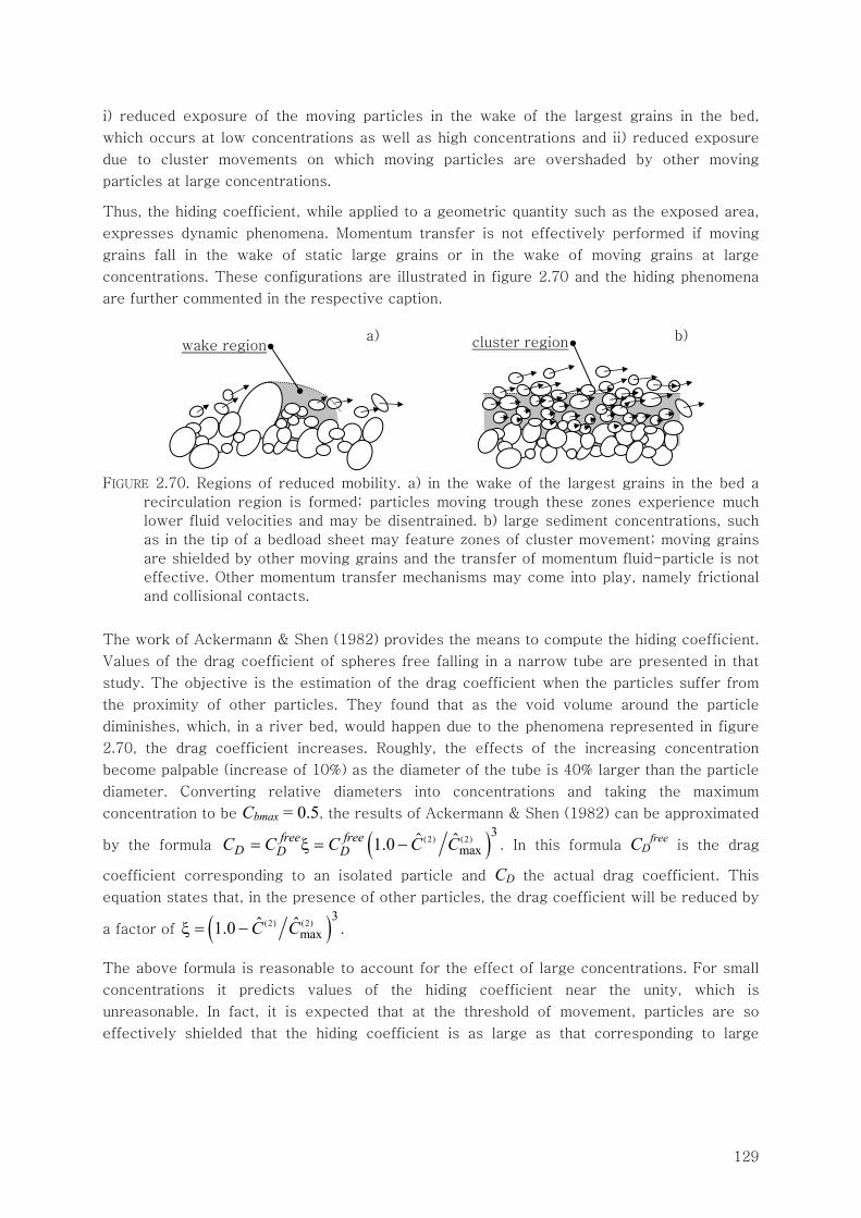
129

i) reduced exposure of the moving particles in the wake of the largest grains in the bed,

which occurs at low concentrations as well as high concentrations and ii) reduced exposure

due to cluster movements on which moving particles are overshaded by other moving

particles at large concentrations.

Thus, the hiding coefficient, while applied to a geometric quantity such as the exposed area,

expresses dynamic phenomena. Momentum transfer is not effectively performed if moving

grains fall in the wake of static large grains or in the wake of moving grains at large

concentrations. These configurations are illustrated in figure 2.70 and the hiding phenomena

are further commented in the respective caption.

FIGURE 2.70. Regions of reduced mobility. a) in the wake of the largest grains in the bed a

recirculation region is formed; particles moving trough these zones experience much

lower fluid velocities and may be disentrained. b) large sediment concentrations, such

as in the tip of a bedload sheet may feature zones of cluster movement; moving grains

are shielded by other moving grains and the transfer of momentum fluid-particle is not

effective. Other momentum transfer mechanisms may come into play, namely frictional

and collisional contacts.

The work of Ackermann & Shen (1982) provides the means to compute the hiding coefficient.

Values of the drag coefficient of spheres free falling in a narrow tube are presented in that

study. The objective is the estimation of the drag coefficient when the particles suffer from

the proximity of other particles. They found that as the void volume around the particle

diminishes, which, in a river bed, would happen due to the phenomena represented in figure

2.70, the drag coefficient increases. Roughly, the effects of the increasing concentration

become palpable (increase of 10%) as the diameter of the tube is 40% larger than the particle

diameter. Converting relative diameters into concentrations and taking the maximum

concentration to be Cbmax = 0.5, the results of Ackermann & Shen (1982) can be approximated

by the formula ( )(2) (2)3

maxˆ ˆ1.0free free

D D DC C C C C= ξ = − . In this formula CDfree

is the drag

coefficient corresponding to an isolated particle and CD the actual drag coefficient. This

equation states that, in the presence of other particles, the drag coefficient will be reduced by

a factor of ( )(2) (2)3

maxˆ ˆ1.0 C Cξ = − .

The above formula is reasonable to account for the effect of large concentrations. For small

concentrations it predicts values of the hiding coefficient near the unity, which is

unreasonable. In fact, it is expected that at the threshold of movement, particles are so

effectively shielded that the hiding coefficient is as large as that corresponding to large

wake region cluster region a) b)

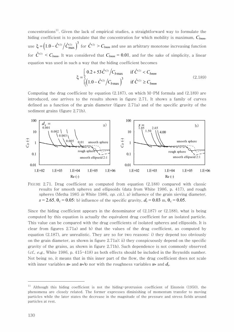
130

concentrations11. Given the lack of empirical studies, a straightforward way to formulate the

hiding coefficient is to postulate that the concentration for which mobility is maximum, Cbmm,

use ( )(2) (2)3

maxˆ ˆ1.0 C Cξ = − for

(2)C > Cbmm and use an arbitrary monotone increasing function

for (2)C < Cbmm. It was considered that Cbmm = 0.01, and for the sake of simplicity, a linear

equation was used in such a way that the hiding coefficient becomes

( )(2) (2)

(2) (2)

max3

max

ˆ ˆ0.2 53 if

ˆ ˆ1.0 if

b bmm

b bmm

C C C C

C C C C

⎧ + <⎪ξ = ⎨− ≥⎪⎩

(2.189)

Computing the drag coefficient by equation (2.187), on which M-PM formula and (2.189) are

introduced, one arrives to the results shown in figure 2.71. It shows a family of curves

defined as a function of the grain diameter (figure 2.71a) and of the specific gravity of the

sediment grains (figure 2.71b).

0.01

0.1

1

10

100

1.E+02 1.E+03 1.E+04 1.E+05 1.E+06Re (-)

CD

(-)

0.0010.002

0.0030.005 0.01 smooth sphere

smooth ellipsoid 2:1

rough sphere

0.01

0.1

1

10

100

1.E+02 1.E+03 1.E+04 1.E+05 1.E+06Re (-)

CD

(-)

1.051.50

2.654.00

smooth sphere

smooth ellipsoid 2:1rough sphere

FIGURE 2.71. Drag coefficient as computed from equation (2.188) compared with classic

results for smooth spheres and ellipsoids (data from White 1986, p. 417), and rough

spheres (Metha 1985 in White 1986, op. cit.). a) influence of the grain sieving diameter,

s = 2.65, θc = 0.05; b) influence of the specific gravity, ds = 0.03 m, θc = 0.05.

Since the hiding coefficient appears in the denominator of (2.187) or (2.188), what is being

computed by this equation is actually the equivalent drag coefficient for an isolated particle.

This value can be compared with the drag coefficients of isolated spheres and ellipsoids. It is

clear from figures 2.71a) and b) that the values of the drag coefficient, as computed by

equation (2.187), are unrealistic. They are so for two reasons: i) they depend too obviously

on the grain diameter, as shown in figure 2.71a); ii) they conspicuously depend on the specific

gravity of the grains, as shown in figure 2.71b). Such dependence is not commonly observed

(cf., e.g., White 1986, p. 415-418) as both effects should be included in the Reynolds number.

Not being so, it means that in this inner part of the flow, the drag coefficient does not scale

with inner variables u* and u*/υ nor with the roughness variables u* and ds.

11 Although this hiding coefficient is not the hiding-protrusion coefficient of Einstein (1950), the

phenomena are closely related. The former expresses diminishing of momentum transfer to moving

particles while the later states the decrease in the magnitude of the pressure and stress fields around

particles at rest.

a) b)sd = s =

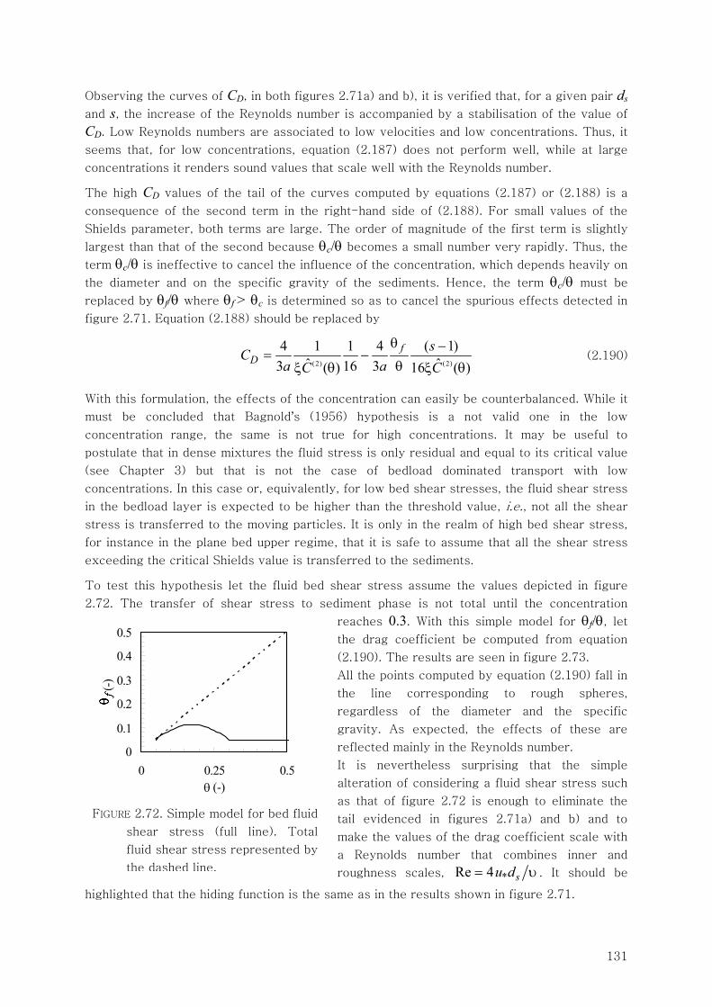
131

0

0.1

0.2

0.3

0.4

0.5

0 0.25 0.5θ (-)

f (-)

FIGURE 2.72. Simple model for bed fluid

shear stress (full line). Total

fluid shear stress represented by

the dashed line.

Observing the curves of CD, in both figures 2.71a) and b), it is verified that, for a given pair ds

and s, the increase of the Reynolds number is accompanied by a stabilisation of the value of

CD. Low Reynolds numbers are associated to low velocities and low concentrations. Thus, it

seems that, for low concentrations, equation (2.187) does not perform well, while at large

concentrations it renders sound values that scale well with the Reynolds number.

The high CD values of the tail of the curves computed by equations (2.187) or (2.188) is a

consequence of the second term in the right-hand side of (2.188). For small values of the

Shields parameter, both terms are large. The order of magnitude of the first term is slightly

largest than that of the second because θc/θ becomes a small number very rapidly. Thus, the

term θc/θ is ineffective to cancel the influence of the concentration, which depends heavily on

the diameter and on the specific gravity of the sediments. Hence, the term θc/θ must be

replaced by θf/θ where θf > θc is determined so as to cancel the spurious effects detected in

figure 2.71. Equation (2.188) should be replaced by

(2) (2)

4 1 1 4 ( 1)ˆ ˆ3 16 3( ) 16 ( )

fD

sCa aC C

θ −= −

θξ θ ξ θ (2.190)

With this formulation, the effects of the concentration can easily be counterbalanced. While it

must be concluded that Bagnold’s (1956) hypothesis is a not valid one in the low

concentration range, the same is not true for high concentrations. It may be useful to

postulate that in dense mixtures the fluid stress is only residual and equal to its critical value

(see Chapter 3) but that is not the case of bedload dominated transport with low

concentrations. In this case or, equivalently, for low bed shear stresses, the fluid shear stress

in the bedload layer is expected to be higher than the threshold value, i.e., not all the shear

stress is transferred to the moving particles. It is only in the realm of high bed shear stress,

for instance in the plane bed upper regime, that it is safe to assume that all the shear stress

exceeding the critical Shields value is transferred to the sediments.

To test this hypothesis let the fluid bed shear stress assume the values depicted in figure

2.72. The transfer of shear stress to sediment phase is not total until the concentration

reaches 0.3. With this simple model for θf/θ, let

the drag coefficient be computed from equation

(2.190). The results are seen in figure 2.73.

All the points computed by equation (2.190) fall in

the line corresponding to rough spheres,

regardless of the diameter and the specific

gravity. As expected, the effects of these are

reflected mainly in the Reynolds number.

It is nevertheless surprising that the simple

alteration of considering a fluid shear stress such

as that of figure 2.72 is enough to eliminate the

tail evidenced in figures 2.71a) and b) and to

make the values of the drag coefficient scale with

a Reynolds number that combines inner and

roughness scales, *Re 4 su d= υ . It should be

highlighted that the hiding function is the same as in the results shown in figure 2.71.

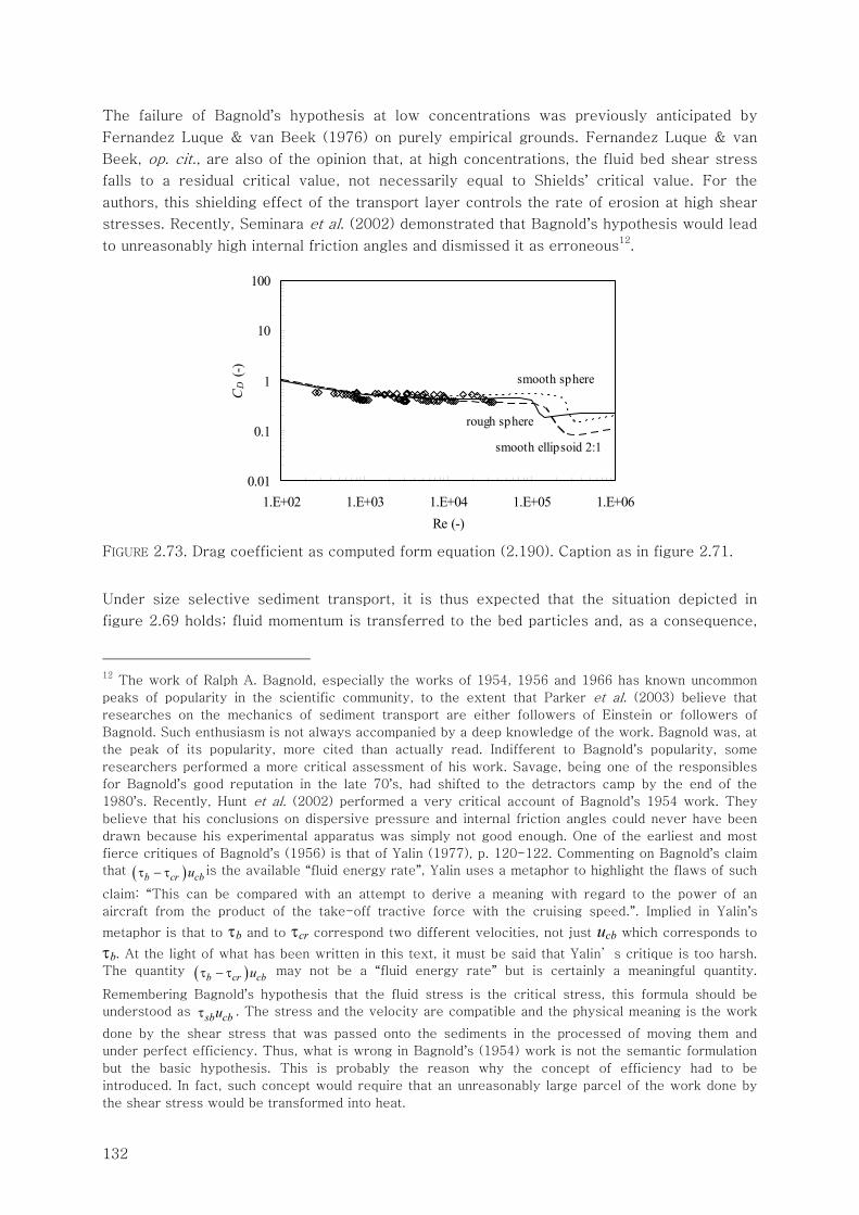
132

The failure of Bagnold’s hypothesis at low concentrations was previously anticipated by

Fernandez Luque & van Beek (1976) on purely empirical grounds. Fernandez Luque & van

Beek, op. cit., are also of the opinion that, at high concentrations, the fluid bed shear stress

falls to a residual critical value, not necessarily equal to Shields’ critical value. For the

authors, this shielding effect of the transport layer controls the rate of erosion at high shear

stresses. Recently, Seminara et al. (2002) demonstrated that Bagnold’s hypothesis would lead

to unreasonably high internal friction angles and dismissed it as erroneous12.

0.01

0.1

1

10

100

1.E+02 1.E+03 1.E+04 1.E+05 1.E+06Re (-)

CD

(-)

smooth sphere

smooth ellipsoid 2:1

rough sphere

FIGURE 2.73. Drag coefficient as computed form equation (2.190). Caption as in figure 2.71.

Under size selective sediment transport, it is thus expected that the situation depicted in

figure 2.69 holds; fluid momentum is transferred to the bed particles and, as a consequence,

12 The work of Ralph A. Bagnold, especially the works of 1954, 1956 and 1966 has known uncommon

peaks of popularity in the scientific community, to the extent that Parker et al. (2003) believe that

researches on the mechanics of sediment transport are either followers of Einstein or followers of

Bagnold. Such enthusiasm is not always accompanied by a deep knowledge of the work. Bagnold was, at

the peak of its popularity, more cited than actually read. Indifferent to Bagnold’s popularity, some

researchers performed a more critical assessment of his work. Savage, being one of the responsibles

for Bagnold’s good reputation in the late 70’s, had shifted to the detractors camp by the end of the

1980’s. Recently, Hunt et al. (2002) performed a very critical account of Bagnold’s 1954 work. They

believe that his conclusions on dispersive pressure and internal friction angles could never have been

drawn because his experimental apparatus was simply not good enough. One of the earliest and most

fierce critiques of Bagnold’s (1956) is that of Yalin (1977), p. 120-122. Commenting on Bagnold’s claim

that ( )b cr cbuτ − τ is the available “fluid energy rate”, Yalin uses a metaphor to highlight the flaws of such

claim: “This can be compared with an attempt to derive a meaning with regard to the power of an

aircraft from the product of the take-off tractive force with the cruising speed.”. Implied in Yalin’s

metaphor is that to τb and to τcr correspond two different velocities, not just ucb which corresponds to

τb. At the light of what has been written in this text, it must be said that Yalin’ s critique is too harsh.

The quantity ( )b cr cbuτ − τ may not be a “fluid energy rate” but is certainly a meaningful quantity.

Remembering Bagnold’s hypothesis that the fluid stress is the critical stress, this formula should be

understood as sb cbuτ . The stress and the velocity are compatible and the physical meaning is the work

done by the shear stress that was passed onto the sediments in the processed of moving them and

under perfect efficiency. Thus, what is wrong in Bagnold’s (1954) work is not the semantic formulation

but the basic hypothesis. This is probably the reason why the concept of efficiency had to be

introduced. In fact, such concept would require that an unreasonably large parcel of the work done by

the shear stress would be transformed into heat.

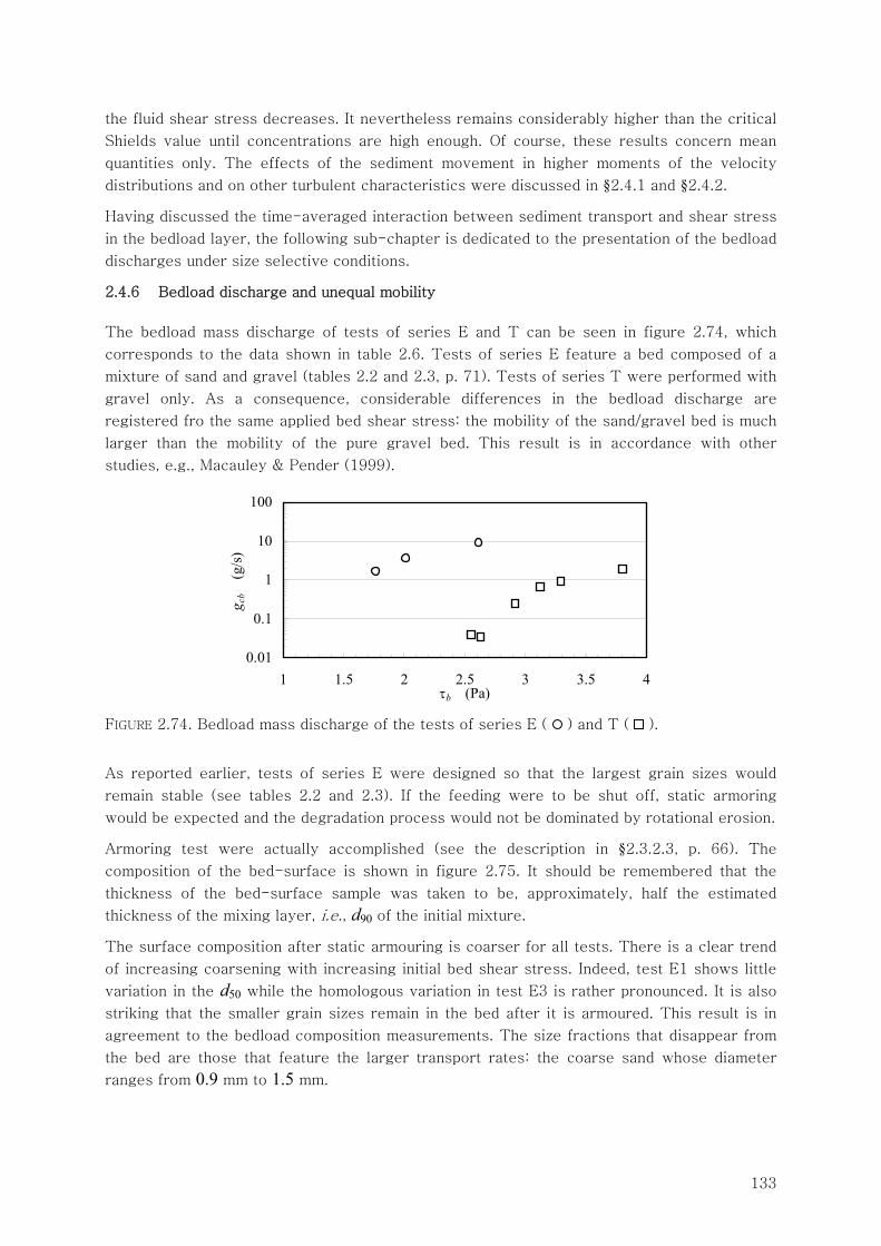
133

the fluid shear stress decreases. It nevertheless remains considerably higher than the critical

Shields value until concentrations are high enough. Of course, these results concern mean

quantities only. The effects of the sediment movement in higher moments of the velocity

distributions and on other turbulent characteristics were discussed in §2.4.1 and §2.4.2.

Having discussed the time-averaged interaction between sediment transport and shear stress

in the bedload layer, the following sub-chapter is dedicated to the presentation of the bedload

discharges under size selective conditions.

2.4.6 Bedload discharge and unequal mobility

The bedload mass discharge of tests of series E and T can be seen in figure 2.74, which

corresponds to the data shown in table 2.6. Tests of series E feature a bed composed of a

mixture of sand and gravel (tables 2.2 and 2.3, p. 71). Tests of series T were performed with

gravel only. As a consequence, considerable differences in the bedload discharge are

registered fro the same applied bed shear stress: the mobility of the sand/gravel bed is much

larger than the mobility of the pure gravel bed. This result is in accordance with other

studies, e.g., Macauley & Pender (1999).

0.01

0.1

1

10

100

1 1.5 2 2.5 3 3.5 4τb (Pa)

g cb

(g

/s)

FIGURE 2.74. Bedload mass discharge of the tests of series E ( ) and T ( ).

As reported earlier, tests of series E were designed so that the largest grain sizes would

remain stable (see tables 2.2 and 2.3). If the feeding were to be shut off, static armoring

would be expected and the degradation process would not be dominated by rotational erosion.

Armoring test were actually accomplished (see the description in §2.3.2.3, p. 66). The

composition of the bed-surface is shown in figure 2.75. It should be remembered that the

thickness of the bed-surface sample was taken to be, approximately, half the estimated

thickness of the mixing layer, i.e., d90 of the initial mixture.

The surface composition after static armouring is coarser for all tests. There is a clear trend

of increasing coarsening with increasing initial bed shear stress. Indeed, test E1 shows little

variation in the d50 while the homologous variation in test E3 is rather pronounced. It is also

striking that the smaller grain sizes remain in the bed after it is armoured. This result is in

agreement to the bedload composition measurements. The size fractions that disappear from

the bed are those that feature the larger transport rates: the coarse sand whose diameter

ranges from 0.9 mm to 1.5 mm.

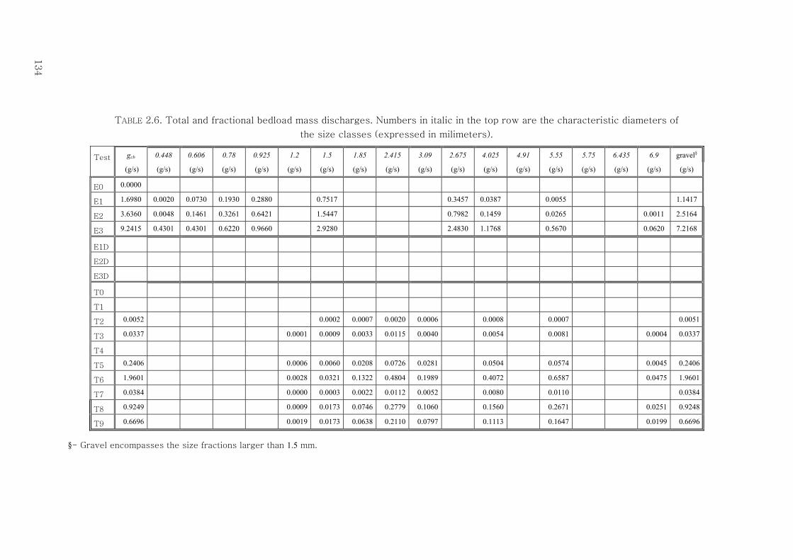
134

TABLE 2.6. Total and fractional bedload mass discharges. Numbers in italic in the top row are the characteristic diameters of

the size classes (expressed in milimeters).

Test gcb 0.448 0.606 0.78 0.925 1.2 1.5 1.85 2.415 3.09 2.675 4.025 4.91 5.55 5.75 6.435 6.9 gravel§

(g/s) (g/s) (g/s) (g/s) (g/s) (g/s) (g/s) (g/s) (g/s) (g/s) (g/s) (g/s) (g/s) (g/s) (g/s) (g/s) (g/s) (g/s)

E0 0.0000

E1 1.6980 0.0020 0.0730 0.1930 0.2880 0.7517 0.3457 0.0387 0.0055 1.1417

E2 3.6360 0.0048 0.1461 0.3261 0.6421 1.5447 0.7982 0.1459 0.0265 0.0011 2.5164

E3 9.2415 0.4301 0.4301 0.6220 0.9660 2.9280 2.4830 1.1768 0.5670 0.0620 7.2168

E1D

E2D

E3D

T0

T1

T2 0.0052 0.0002 0.0007 0.0020 0.0006 0.0008 0.0007 0.0051

T3 0.0337 0.0001 0.0009 0.0033 0.0115 0.0040 0.0054 0.0081 0.0004 0.0337

T4

T5 0.2406 0.0006 0.0060 0.0208 0.0726 0.0281 0.0504 0.0574 0.0045 0.2406

T6 1.9601 0.0028 0.0321 0.1322 0.4804 0.1989 0.4072 0.6587 0.0475 1.9601

T7 0.0384 0.0000 0.0003 0.0022 0.0112 0.0052 0.0080 0.0110 0.0384

T8 0.9249 0.0009 0.0173 0.0746 0.2779 0.1060 0.1560 0.2671 0.0251 0.9248

T9 0.6696 0.0019 0.0173 0.0638 0.2110 0.0797 0.1113 0.1647 0.0199 0.6696

§- Gravel encompasses the size fractions larger than 1.5 mm.

134

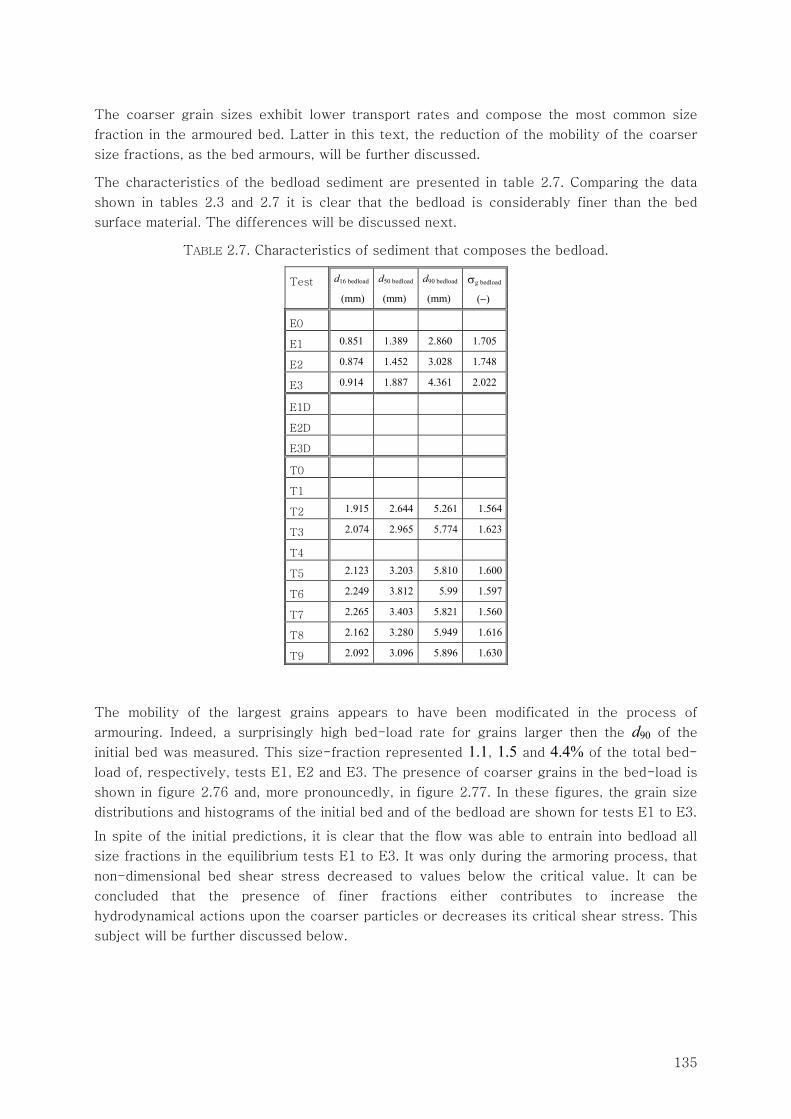
135

The coarser grain sizes exhibit lower transport rates and compose the most common size

fraction in the armoured bed. Latter in this text, the reduction of the mobility of the coarser

size fractions, as the bed armours, will be further discussed.

The characteristics of the bedload sediment are presented in table 2.7. Comparing the data

shown in tables 2.3 and 2.7 it is clear that the bedload is considerably finer than the bed

surface material. The differences will be discussed next.

TABLE 2.7. Characteristics of sediment that composes the bedload.

Test d16 bedload d50 bedload d90 bedload σg bedload

(mm) (mm) (mm) (−)

E0

E1 0.851 1.389 2.860 1.705

E2 0.874 1.452 3.028 1.748

E3 0.914 1.887 4.361 2.022

E1D

E2D

E3D

T0

T1

T2 1.915 2.644 5.261 1.564

T3 2.074 2.965 5.774 1.623

T4

T5 2.123 3.203 5.810 1.600

T6 2.249 3.812 5.99 1.597

T7 2.265 3.403 5.821 1.560

T8 2.162 3.280 5.949 1.616

T9 2.092 3.096 5.896 1.630

The mobility of the largest grains appears to have been modificated in the process of

armouring. Indeed, a surprisingly high bed-load rate for grains larger then the d90 of the

initial bed was measured. This size-fraction represented 1.1, 1.5 and 4.4% of the total bed-

load of, respectively, tests E1, E2 and E3. The presence of coarser grains in the bed-load is

shown in figure 2.76 and, more pronouncedly, in figure 2.77. In these figures, the grain size

distributions and histograms of the initial bed and of the bedload are shown for tests E1 to E3.

In spite of the initial predictions, it is clear that the flow was able to entrain into bedload all

size fractions in the equilibrium tests E1 to E3. It was only during the armoring process, that

non-dimensional bed shear stress decreased to values below the critical value. It can be

concluded that the presence of finer fractions either contributes to increase the

hydrodynamical actions upon the coarser particles or decreases its critical shear stress. This

subject will be further discussed below.

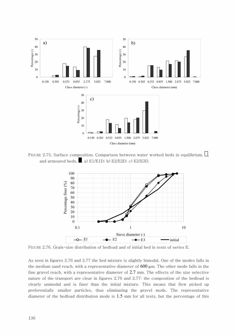
136

0

10

20

30

40

50

0.150 0.303 0.533 0.855 2.175 5.025 7.000

Class diameter (-)

Perc

enta

ge (-

)

0

10

20

30

40

50

0.150 0.303 0.533 0.855 1.500 2.675 5.025 7.000

Class diameter (mm)

Perc

enta

ge (-

)

0

10

20

30

40

50

0.150 0.303 0.533 0.855 1.500 2.675 5.025 7.000

Class diameter (mm)

Perc

enta

ge (-

)

FIGURE 2.75. Surface composition. Comparison between water worked beds in equilibrium, ,

and armoured beds, . a) E1/E1D; b) E2/E2D; c) E3/E3D.

0102030405060708090

100

0.1 1 10

Sieve diameter (-)

Perc

enta

ge fi

ner (

%)

E3 E4 E3 initial

FIGURE 2.76. Grain-size distribution of bedload and of initial bed in tests of series E.

As seen in figures 2.76 and 2.77 the bed mixture is slightly bimodal. One of the modes falls in

the medium sand reach, with a representative diameter of 600 μm. The other mode falls in the

fine gravel reach, with a representative diameter of 2.7 mm. The effects of the size selective

nature of the transport are clear in figures 2.76 and 2.77: the composition of the bedload is

clearly unimodal and is finer than the initial mixture. This means that flow picked up

preferentially smaller particles, thus eliminating the gravel mode. The representative

diameter of the bedload distribution mode is 1.5 mm for all tests, but the percentage of this

a) b)

c)

E1 E2

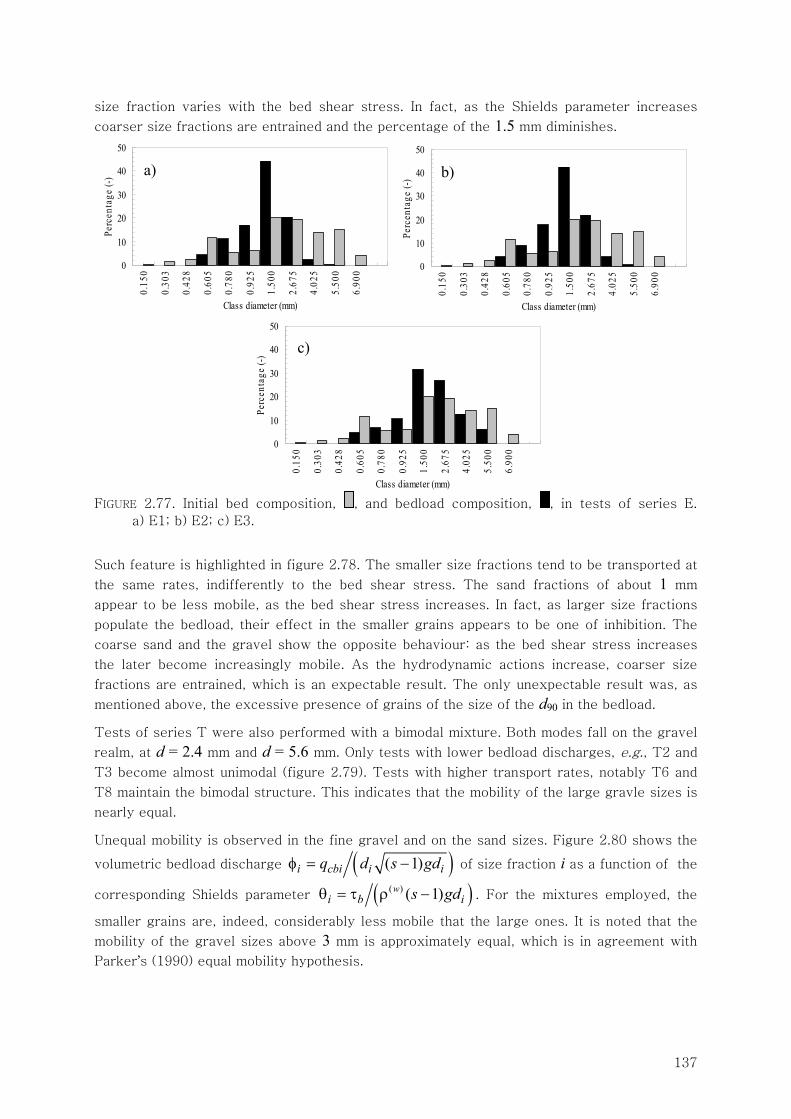
137

size fraction varies with the bed shear stress. In fact, as the Shields parameter increases

coarser size fractions are entrained and the percentage of the 1.5 mm diminishes.

0

10

20

30

40

500.

150

0.30

3

0.42

8

0.60

5

0.78

0

0.92

5

1.50

0

2.67

5

4.02

5

5.50

0

6.90

0

Class diameter (mm)

Perc

enta

ge (-

)

0

10

20

30

40

50

0.15

0

0.30

3

0.42

8

0.60

5

0.78

0

0.92

5

1.50

0

2.67

5

4.02

5

5.50

0

6.90

0

Class diameter (mm)

Perc

enta

ge (-

)

0

10

20

30

40

50

0.15

0

0.30

3

0.42

8

0.60

5

0.78

0

0.92

5

1.50

0

2.67

5

4.02

5

5.50

0

6.90

0

Class diameter (mm)

Perc

enta

ge (-

)

FIGURE 2.77. Initial bed composition, , and bedload composition, , in tests of series E.

a) E1; b) E2; c) E3.

Such feature is highlighted in figure 2.78. The smaller size fractions tend to be transported at

the same rates, indifferently to the bed shear stress. The sand fractions of about 1 mm

appear to be less mobile, as the bed shear stress increases. In fact, as larger size fractions

populate the bedload, their effect in the smaller grains appears to be one of inhibition. The

coarse sand and the gravel show the opposite behaviour: as the bed shear stress increases

the later become increasingly mobile. As the hydrodynamic actions increase, coarser size

fractions are entrained, which is an expectable result. The only unexpectable result was, as

mentioned above, the excessive presence of grains of the size of the d90 in the bedload.

Tests of series T were also performed with a bimodal mixture. Both modes fall on the gravel

realm, at d = 2.4 mm and d = 5.6 mm. Only tests with lower bedload discharges, e.g., T2 and

T3 become almost unimodal (figure 2.79). Tests with higher transport rates, notably T6 and

T8 maintain the bimodal structure. This indicates that the mobility of the large gravle sizes is

nearly equal.

Unequal mobility is observed in the fine gravel and on the sand sizes. Figure 2.80 shows the

volumetric bedload discharge ( )( 1)i cbi i iq d s gdφ = − of size fraction i as a function of the

corresponding Shields parameter ( )( ) ( 1)wi b is gdθ = τ ρ − . For the mixtures employed, the

smaller grains are, indeed, considerably less mobile that the large ones. It is noted that the

mobility of the gravel sizes above 3 mm is approximately equal, which is in agreement with

Parker’s (1990) equal mobility hypothesis.

a) b)

c)

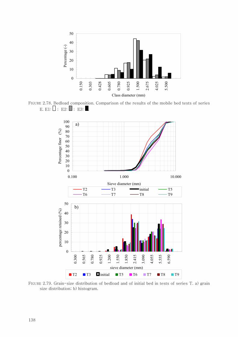
138

0

10

20

30

40

50

0.15

0

0.30

3

0.42

8

0.60

5

0.78

0

0.92

5

1.50

0

2.67

5

4.02

5

5.50

0

Class diameter (mm)

Perc

enta

ge (-

)

FIGURE 2.78. Bedload composition. Comparison of the results of the mobile bed tests of series

E. E1: ; E2: ; E3: .

0102030405060708090

100

0.100 1.000 10.000

Sieve diameter (mm)

Perc

enta

ge fi

ner

(%)

T2 T3 initial T5T6 T7 T8 T9

0

10

20

30

40

50

0.30

0

0.56

5

0.78

0

0.92

5

1.20

0

1.55

0

1.85

0

2.41

5

3.09

0

4.05

5

5.55

5

6.59

0

sieve diameter (mm)

perc

enta

ge re

tain

ed (%

)

T2 T3 initial T5 T6 T7 T8 T9

FIGURE 2.79. Grain-size distribution of bedload and of initial bed in tests of series T. a) grain

size distribution; b) histogram.

a)

b)

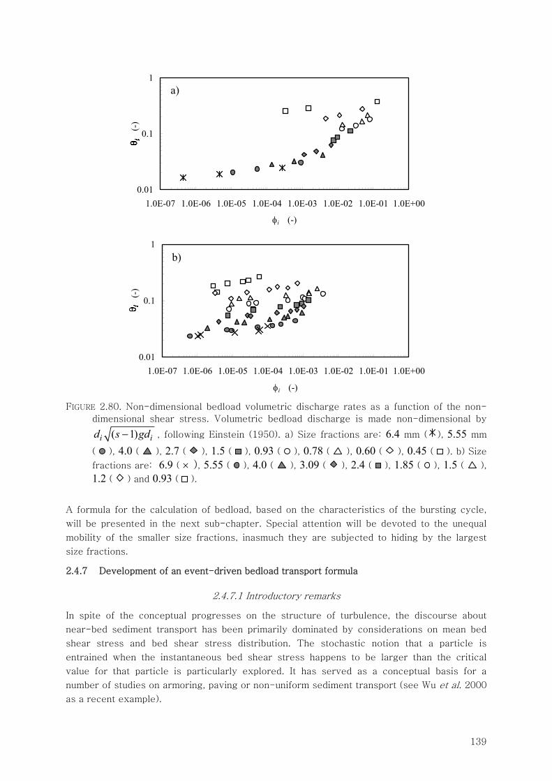
139

0.01

0.1

1

1.0E-07 1.0E-06 1.0E-05 1.0E-04 1.0E-03 1.0E-02 1.0E-01 1.0E+00

φi (-)

Π i

(-)

0.01

0.1

1

1.0E-07 1.0E-06 1.0E-05 1.0E-04 1.0E-03 1.0E-02 1.0E-01 1.0E+00

φi (-)

Π i

(-)

FIGURE 2.80. Non-dimensional bedload volumetric discharge rates as a function of the non-

dimensional shear stress. Volumetric bedload discharge is made non-dimensional by

( 1)i id s gd− , following Einstein (1950). a) Size fractions are: 6.4 mm ( ), 5.55 mm

( ), 4.0 ( ), 2.7 ( ), 1.5 ( ), 0.93 ( ), 0.78 ( ), 0.60 ( ), 0.45 ( ). b) Size

fractions are: 6.9 ( × ), 5.55 ( ), 4.0 ( ), 3.09 ( ), 2.4 ( ), 1.85 ( ), 1.5 ( ),

1.2 ( ) and 0.93 ( ).

A formula for the calculation of bedload, based on the characteristics of the bursting cycle,

will be presented in the next sub-chapter. Special attention will be devoted to the unequal

mobility of the smaller size fractions, inasmuch they are subjected to hiding by the largest

size fractions.

2.4.7 Development of an event-driven bedload transport formula

2.4.7.1 Introductory remarks

In spite of the conceptual progresses on the structure of turbulence, the discourse about

near-bed sediment transport has been primarily dominated by considerations on mean bed

shear stress and bed shear stress distribution. The stochastic notion that a particle is

entrained when the instantaneous bed shear stress happens to be larger than the critical

value for that particle is particularly explored. It has served as a conceptual basis for a

number of studies on armoring, paving or non-uniform sediment transport (see Wu et al. 2000

as a recent example).

a)

b)

140

Yet, formulas based on a critical shear stress, eventually corrected by a hiding (for small

grain sizes) or exposure (for large grain sizes) coefficient, are not suitable to tackle problems

such as that identified in §2.4.6: gravel sizes, of the order of d90, are immobile if the bed is

starved of finer fractions but are mobile is surrounded of moving fine sediment. In both cases,

the theoretical non-dimensional critical shear stress is larger than the applied non-

dimensional shear stress applied to that size fraction.

Apparently, the mobility of a coarse particle increases in the presence of finer fractions in the

bedload. In an armored bed, a given size fraction, whose applied shear stress is well below

threshold, becomes mobile as fine sediment is re-introduced in the system. Two hypotheses,

illustrated in figures 2.81 to 2.82, can be put forward to explain this feature.

The stability of the individual large grains in a mobile bed is the key issue addressed by

hypothesis one. If a large amount of fine sediment is removed from the bed in the vicinity of a

large particle, this particle may instabilize, thus triggering its movement, or displace itself

only to be stopped at an overexposed location. This would represent a decrease in the critical

shear stress (figure 2.81).

Hypothesis two was addressed in §2.4.1 and §2.4.2, pp. 73 and 106, respectively. The

hypothesis that bed movement may introduce changes in the structure of turbulence in the

roughness sub-layer was partially discarded. Mean quantities and second-order moments are

not affected. Yet, it is possible that subtle differences in the third-order moments, visible in

the flux of turbulent kinetic energy and in the maximum magnitude of the turbulent sweep

events, may affect the magnitude of the momentum transfer from the mean flow to the

particles. Hence, it is possible that the mobility of the larger fractions in the presence of finer

ones is associated to the increase of maximum magnitude of uv , as shown in figure 2.82. It is

not clear, however, if the increased mobility is a cause or an effect of the increased intensity

of the coherent events.

The hiding of the smaller grain sizes is another aspect to be addressed by the bedload model.

It was seen, in §2.4.5, p. 123, that the drag felt by the smaller particles is much smaller when

placed in the wakes of the larger particles. In addition, it was shown the bed shear stress is

not instantly consumed in the transport of the bedload as soon as the particles start to move.

On the contrary, the bed shear stress associated to sediment transport increases gradually.

These aspects can be explicitly addressed if it is considered that the bedload is driven by

coherent turbulent events, namely the sweep event (see §2.4.2).

Devising a formula for the bedload discharge, conceptualized as an even-driven phenomenon

is the objective of this sub-chapter.

The hypothesis that the entrainment and the transport of sediment particles are directly

related to a turbulent bursting cycle is as old as the description of the bursting cycle itself.

Prior to the concept of turbulent events, Sutherland (1967), performed a landmark study of

event-driven bedload transport. The basic idea underlying Sutherland’s work is illustrated in

figure 2.83: a mass of fluid, which, in a turbulent flow, takes the form of a coherent turbulent

structure, impinges on the bed thus locally increasing the hydrodynamic actions upon the

particles past their critical stability values and consequently promoting its entrainment.

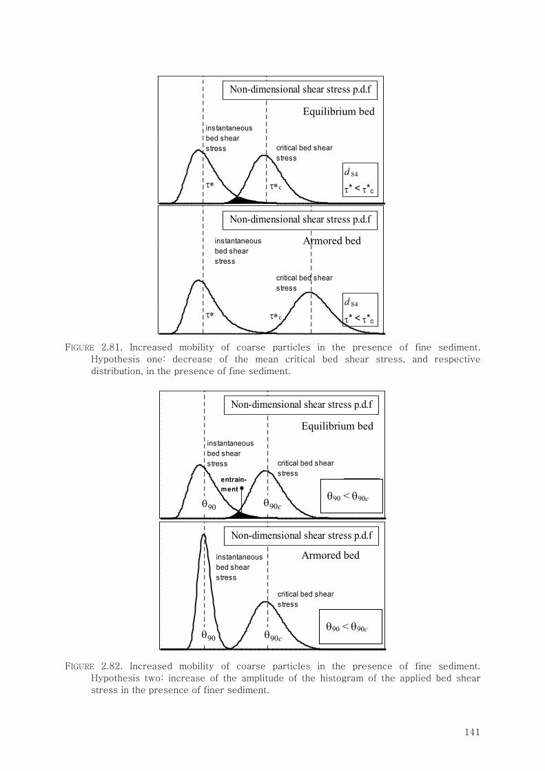
141

FIGURE 2.81. Increased mobility of coarse particles in the presence of fine sediment.

Hypothesis one: decrease of the mean critical bed shear stress, and respective

distribution, in the presence of fine sediment.

FIGURE 2.82. Increased mobility of coarse particles in the presence of fine sediment.

Hypothesis two: increase of the amplitude of the histogram of the applied bed shear

stress in the presence of finer sediment.

instantaneous bed shear stress critical bed shear

stress

τ∗ τ∗c

Non-dimensional shear stress p.d.f

d 84

τ* < τ*c

instantaneous bed shear stress

critical bed shear stress

τ∗ τ∗c

Non-dimensional shear stress p.d.f

d 84

τ* < τ*c

Equilibrium bed

Armored bed

instantaneous bed shear stress critical bed shear

stress

τ∗ τ∗c

Non-dimensional shear stress p.d.f

d 84

τ* < τ*c

entrain-ment

instantaneous bed shear stress

critical bed shear stress

τ∗ τ∗c

Non-dimensional shear stress p.d.f

d 84

τ* < τ*c

Equilibrium bed

Armored bed

θ90 < θ90c

θ90 < θ90c

90θ

90θ 90cθ

90cθ

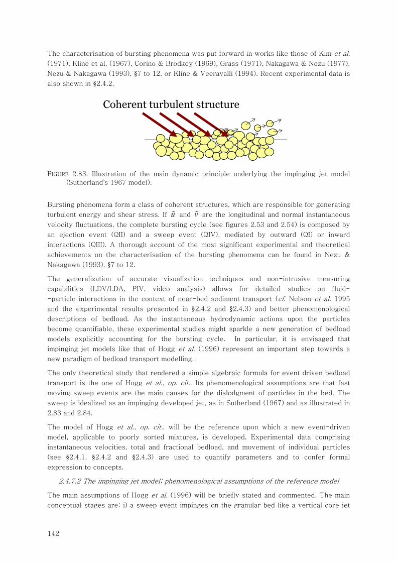
142

The characterisation of bursting phenomena was put forward in works like those of Kim et al.

(1971), Kline et al. (1967), Corino & Brodkey (1969), Grass (1971), Nakagawa & Nezu (1977),

Nezu & Nakagawa (1993), §7 to 12, or Kline & Veeravalli (1994). Recent experimental data is

also shown in §2.4.2.

FIGURE 2.83. Illustration of the main dynamic principle underlying the impinging jet model

(Sutherland’s 1967 model).

Bursting phenomena form a class of coherent structures, which are responsible for generating

turbulent energy and shear stress. If u and v are the longitudinal and normal instantaneous

velocity fluctuations, the complete bursting cycle (see figures 2.53 and 2.54) is composed by

an ejection event (QII) and a sweep event (QIV), mediated by outward (QI) or inward

interactions (QIII). A thorough account of the most significant experimental and theoretical

achievements on the characterisation of the bursting phenomena can be found in Nezu &

Nakagawa (1993), §7 to 12.

The generalization of accurate visualization techniques and non-intrusive measuring

capabilities (LDV/LDA, PIV, video analysis) allows for detailed studies on fluid-

-particle interactions in the context of near-bed sediment transport (cf. Nelson et al. 1995

and the experimental results presented in §2.4.2 and §2.4.3) and better phenomenological

descriptions of bedload. As the instantaneous hydrodynamic actions upon the particles

become quantifiable, these experimental studies might sparkle a new generation of bedload

models explicitly accounting for the bursting cycle. In particular, it is envisaged that

impinging jet models like that of Hogg et al. (1996) represent an important step towards a

new paradigm of bedload transport modelling.

The only theoretical study that rendered a simple algebraic formula for event driven bedload

transport is the one of Hogg et al., op. cit.. Its phenomenological assumptions are that fast

moving sweep events are the main causes for the dislodgment of particles in the bed. The

sweep is idealized as an impinging developed jet, as in Sutherland (1967) and as illustrated in

2.83 and 2.84.

The model of Hogg et al., op. cit., will be the reference upon which a new event-driven

model, applicable to poorly sorted mixtures, is developed. Experimental data comprising

instantaneous velocities, total and fractional bedload, and movement of individual particles

(see §2.4.1, §2.4.2 and §2.4.3) are used to quantify parameters and to confer formal

expression to concepts.

2.4.7.2 The impinging jet model; phenomenological assumptions of the reference model

The main assumptions of Hogg et al. (1996) will be briefly stated and commented. The main

conceptual stages are: i) a sweep event impinges on the granular bed like a vertical core jet

Coherent turbulent structure

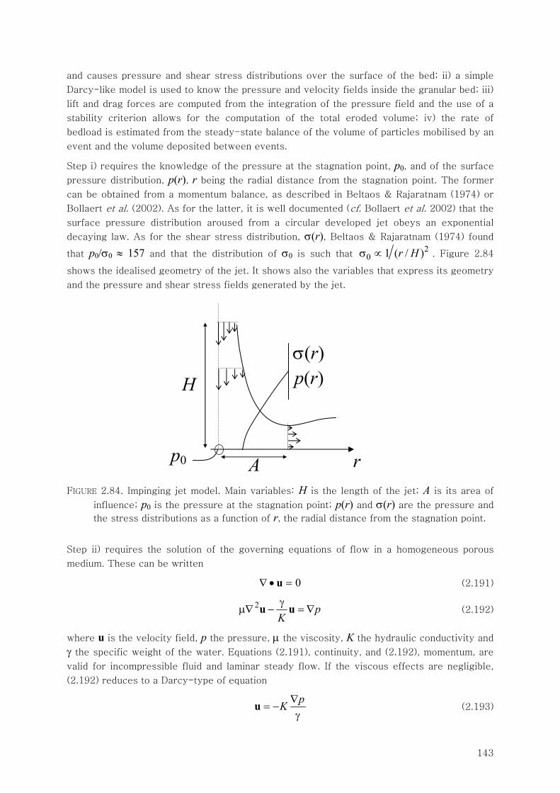
143

and causes pressure and shear stress distributions over the surface of the bed; ii) a simple

Darcy-like model is used to know the pressure and velocity fields inside the granular bed; iii)

lift and drag forces are computed from the integration of the pressure field and the use of a

stability criterion allows for the computation of the total eroded volume; iv) the rate of

bedload is estimated from the steady-state balance of the volume of particles mobilised by an

event and the volume deposited between events.

Step i) requires the knowledge of the pressure at the stagnation point, p0, and of the surface

pressure distribution, p(r), r being the radial distance from the stagnation point. The former

can be obtained from a momentum balance, as described in Beltaos & Rajaratnam (1974) or

Bollaert et al. (2002). As for the latter, it is well documented (cf. Bollaert et al. 2002) that the

surface pressure distribution aroused from a circular developed jet obeys an exponential

decaying law. As for the shear stress distribution, σ(r), Beltaos & Rajaratnam (1974) found

that p0/σ0 ≈ 157 and that the distribution of σ0 is such that 2

0 1 ( / )r Hσ ∝ . Figure 2.84

shows the idealised geometry of the jet. It shows also the variables that express its geometry

and the pressure and shear stress fields generated by the jet.

FIGURE 2.84. Impinging jet model. Main variables: H is the length of the jet; A is its area of

influence; p0 is the pressure at the stagnation point; p(r) and σ(r) are the pressure and

the stress distributions as a function of r, the radial distance from the stagnation point.

Step ii) requires the solution of the governing equations of flow in a homogeneous porous

medium. These can be written

0=•∇ u (2.191)

pK

∇=γ

−∇μ uu2 (2.192)

where u is the velocity field, p the pressure, μ the viscosity, K the hydraulic conductivity and

γ the specific weight of the water. Equations (2.191), continuity, and (2.192), momentum, are

valid for incompressible fluid and laminar steady flow. If the viscous effects are negligible,

(2.192) reduces to a Darcy-type of equation

γ

∇−=

pKu (2.193)

H

A p0

p(r)

σ(r)

r

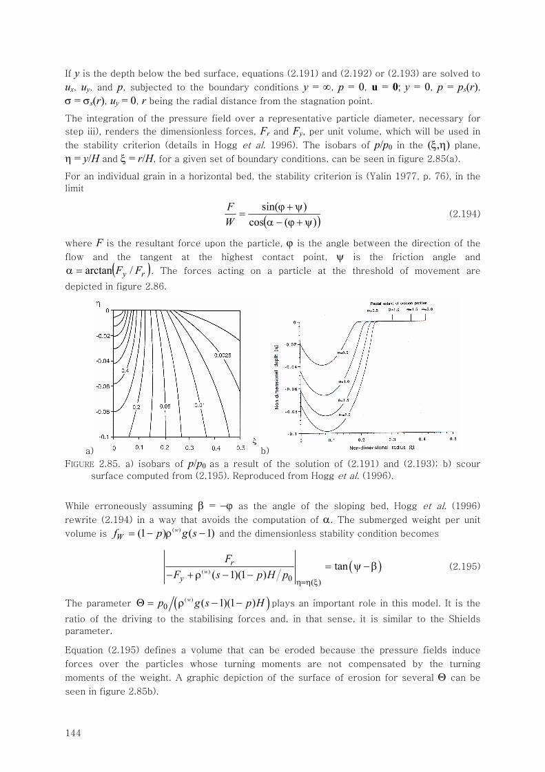
144

If y is the depth below the bed surface, equations (2.191) and (2.192) or (2.193) are solved to

ux, uy, and p, subjected to the boundary conditions y = ∞, p = 0, u = 0; y = 0, p = ps(r), σ = σs(r), uy = 0, r being the radial distance from the stagnation point.

The integration of the pressure field over a representative particle diameter, necessary for

step iii), renders the dimensionless forces, Fr and Fy, per unit volume, which will be used in

the stability criterion (details in Hogg et al. 1996). The isobars of p/p0 in the (ξ,η) plane,

η = y/H and ξ = r/H, for a given set of boundary conditions, can be seen in figure 2.85(a).

For an individual grain in a horizontal bed, the stability criterion is (Yalin 1977, p. 76), in the

limit

( ))(cos)sin(ψ+ϕ−α

ψ+ϕ=

WF

(2.194)

where F is the resultant force upon the particle, ϕ is the angle between the direction of the

flow and the tangent at the highest contact point, ψ is the friction angle and

( )ry FF /arctan=α . The forces acting on a particle at the threshold of movement are

depicted in figure 2.86.

a) b)

FIGURE 2.85. a) isobars of p/p0 as a result of the solution of (2.191) and (2.193); b) scour

surface computed from (2.195). Reproduced from Hogg et al. (1996).

While erroneously assuming β = −ϕ as the angle of the sloping bed, Hogg et al. (1996)

rewrite (2.194) in a way that avoids the computation of α. The submerged weight per unit

volume is ( )(1 ) ( 1)w

Wf p g s= − ρ − and the dimensionless stability condition becomes

( )( )0 ( )

tan( 1)(1 )w

r

y

FF s p H p

η=η ξ

= ψ − β− + ρ − −

(2.195)

The parameter ( )( )0 ( 1)(1 )wp g s p HΘ = ρ − − plays an important role in this model. It is the

ratio of the driving to the stabilising forces and, in that sense, it is similar to the Shields

parameter.

Equation (2.195) defines a volume that can be eroded because the pressure fields induce

forces over the particles whose turning moments are not compensated by the turning

moments of the weight. A graphic depiction of the surface of erosion for several Θ can be

seen in figure 2.85b).

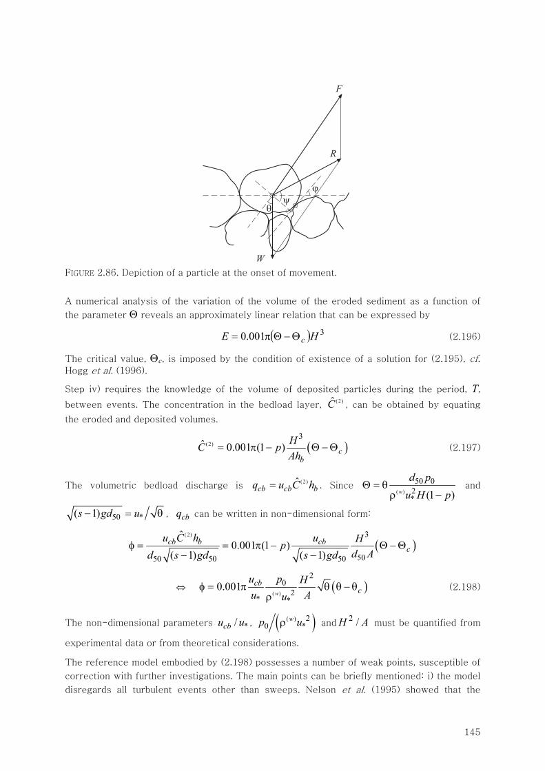
145

FIGURE 2.86. Depiction of a particle at the onset of movement.

A numerical analysis of the variation of the volume of the eroded sediment as a function of

the parameter Θ reveals an approximately linear relation that can be expressed by

( ) 3001.0 HE cΘ−Θπ= (2.196)

The critical value, Θc, is imposed by the condition of existence of a solution for (2.195), cf. Hogg et al. (1996).

Step iv) requires the knowledge of the volume of deposited particles during the period, T,

between events. The concentration in the bedload layer, (2)C , can be obtained by equating

the eroded and deposited volumes.

( )(2)3

ˆ 0.001 (1 ) cb

HC pAh

= π − Θ − Θ (2.197)

The volumetric bedload discharge is (2)ˆ

cb cb bq u C h= . Since ( )

50 02* (1 )w

d pu H p

Θ = θρ −

and

50 *( 1)s gd u− = θ , cbq can be written in non-dimensional form:

( )(2) 3

5050 50 50

ˆ0.001 (1 )

( 1) ( 1)cb b cb

cu C h u Hp

d Ad s gd s gdφ = = π − Θ − Θ

− −

⇔ ( )( )

20

2* *

0.001w

cbc

u p Hu Au

φ = π θ θ − θρ

(2.198)

The non-dimensional parameters */cbu u , ( )( ) 20 *

wp uρ and AH /2 must be quantified from

experimental data or from theoretical considerations.

The reference model embodied by (2.198) possesses a number of weak points, susceptible of

correction with further investigations. The main points can be briefly mentioned: i) the model

disregards all turbulent events other than sweeps. Nelson et al. (1995) showed that the

α

�

�

�

��

�

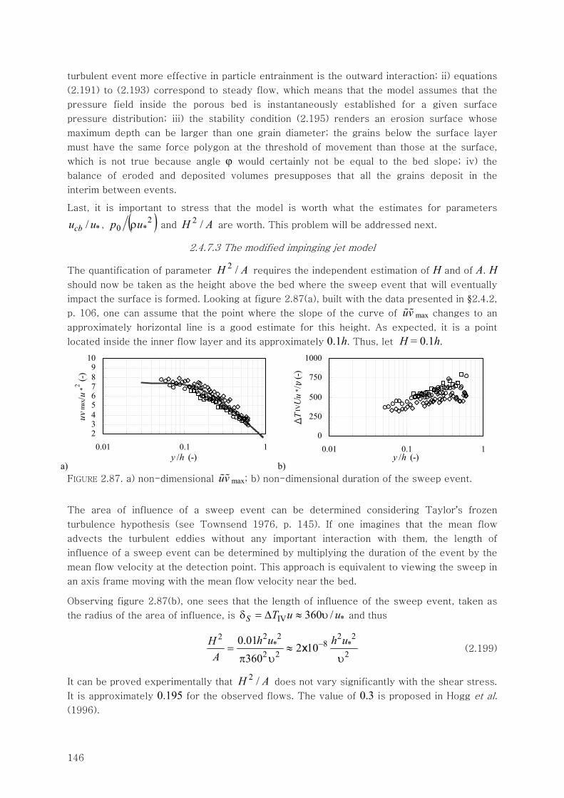
146

turbulent event more effective in particle entrainment is the outward interaction; ii) equations

(2.191) to (2.193) correspond to steady flow, which means that the model assumes that the

pressure field inside the porous bed is instantaneously established for a given surface

pressure distribution; iii) the stability condition (2.195) renders an erosion surface whose

maximum depth can be larger than one grain diameter; the grains below the surface layer

must have the same force polygon at the threshold of movement than those at the surface,

which is not true because angle ϕ would certainly not be equal to the bed slope; iv) the

balance of eroded and deposited volumes presupposes that all the grains deposit in the

interim between events.

Last, it is important to stress that the model is worth what the estimates for parameters

*/cbu u , ( )2*0 up ρ and AH /2

are worth. This problem will be addressed next.

2.4.7.3 The modified impinging jet model

The quantification of parameter AH /2 requires the independent estimation of H and of A. H

should now be taken as the height above the bed where the sweep event that will eventually

impact the surface is formed. Looking at figure 2.87(a), built with the data presented in §2.4.2,

p. 106, one can assume that the point where the slope of the curve of uv max changes to an

approximately horizontal line is a good estimate for this height. As expected, it is a point

located inside the inner flow layer and its approximately 0.1h. Thus, let H = 0.1h.

a)

23456789

10

0.01 0.1 1y /h (-)

uvm

ax/u

*2 (-)

b)

0

250

500

750

1000

0.01 0.1 1y /h (-)

TIV

Uu

* / (-

)

FIGURE 2.87. a) non-dimensional uv max; b) non-dimensional duration of the sweep event.

The area of influence of a sweep event can be determined considering Taylor’s frozen

turbulence hypothesis (see Townsend 1976, p. 145). If one imagines that the mean flow

advects the turbulent eddies without any important interaction with them, the length of

influence of a sweep event can be determined by multiplying the duration of the event by the

mean flow velocity at the detection point. This approach is equivalent to viewing the sweep in

an axis frame moving with the mean flow velocity near the bed.

Observing figure 2.87(b), one sees that the length of influence of the sweep event, taken as

the radius of the area of influence, is IV *360 /S T u uδ = Δ ≈ υ and thus

2 2 2 228* *

2 2 20.01

2 10360

h u h uHA

−= ≈π υ υ

x (2.199)

It can be proved experimentally that AH /2 does not vary significantly with the shear stress.

It is approximately 0.195 for the observed flows. The value of 0.3 is proposed in Hogg et al.

(1996).

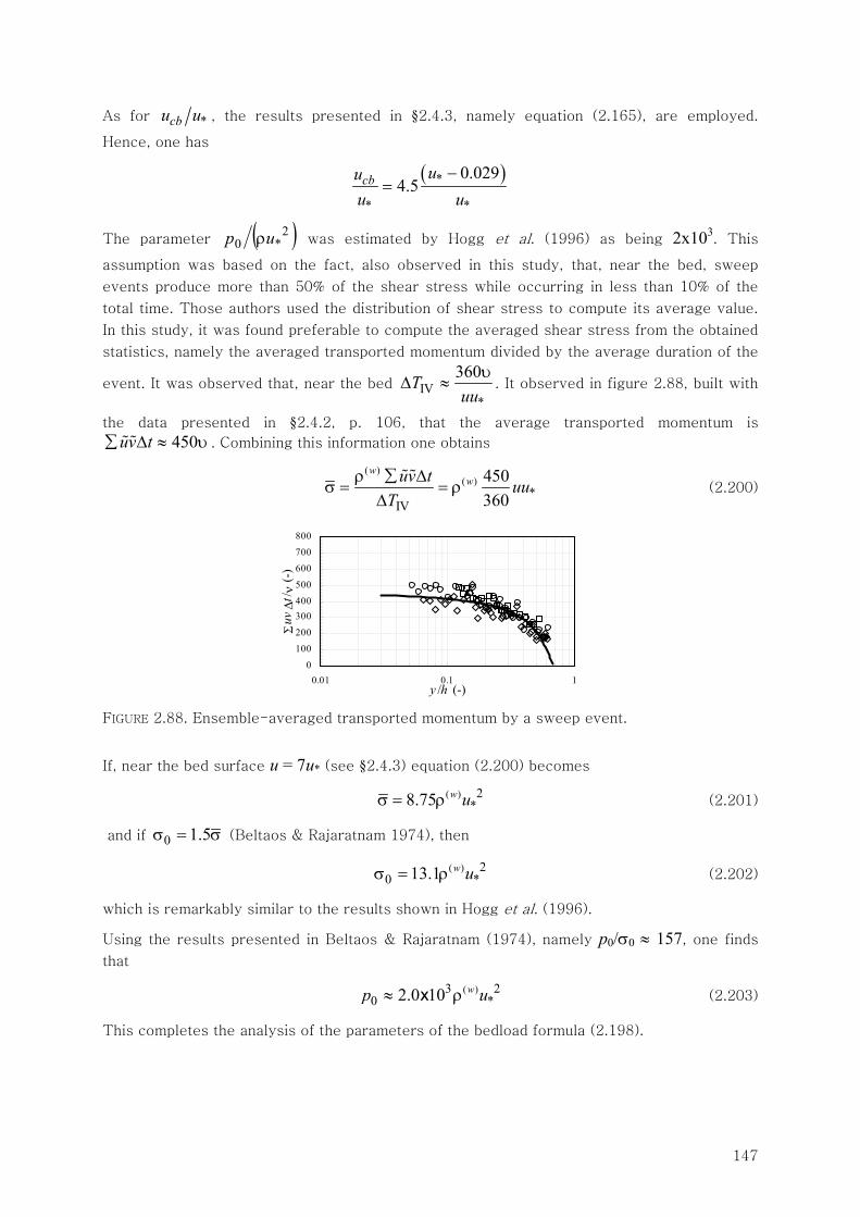
147

As for *cbu u , the results presented in §2.4.3, namely equation (2.165), are employed.

Hence, one has

( )*

* *

0.0294.5cb uu

u u−

=

The parameter ( )2*0 up ρ was estimated by Hogg et al. (1996) as being 2x103

. This

assumption was based on the fact, also observed in this study, that, near the bed, sweep

events produce more than 50% of the shear stress while occurring in less than 10% of the

total time. Those authors used the distribution of shear stress to compute its average value.

In this study, it was found preferable to compute the averaged shear stress from the obtained

statistics, namely the averaged transported momentum divided by the average duration of the

event. It was observed that, near the bed IV*

360Tuu

υΔ ≈ . It observed in figure 2.88, built with

the data presented in §2.4.2, p. 106, that the average transported momentum is

450uv t∑ Δ ≈ υ . Combining this information one obtains

( )( )

*IV

450360

wwuv t uu

Tρ ∑ Δ

σ = = ρΔ

(2.200)

0

100

200

300400

500

600

700

800

0.01 0.1 1y /h (-)

Σuv

Δt/ ν

(-)

FIGURE 2.88. Ensemble-averaged transported momentum by a sweep event.

If, near the bed surface u = 7u* (see §2.4.3) equation (2.200) becomes

( ) 2

*8.75 w uσ = ρ (2.201)

and if 0 1.5σ = σ (Beltaos & Rajaratnam 1974), then

( ) 2

0 *13.1 w uσ = ρ (2.202)

which is remarkably similar to the results shown in Hogg et al. (1996).

Using the results presented in Beltaos & Rajaratnam (1974), namely p0/σ0 ≈ 157, one finds

that

( )3 2

0 *2.0 10 wp u≈ ρx (2.203)

This completes the analysis of the parameters of the bedload formula (2.198).

148

To generalise (2.198) to the transport of granulometric mixtures, it is necessary to calculate

the transport of each size fraction. A first step is diviving the transport in accordance to the

composition of the bed surface. Equation (2.197) becomes

( )(2)3

ˆ 0.001 (1 )i i cb

HC F pAh

= π − Θ − Θ (2.204)

Application of equation (2.204) would cause the bedload to have the composition of the bed

surface, which, as seen in §2.4.6, p. 133, would be erroneous. It is necessary to consider

unequal mobility, especially for the smaller size fractions subjected to hiding, and protrusion

effects. Concerning the later, it is necessary to introduce the possibility of entrainment of a

large particle due to instabilization, even if its mean critical shear stress is greater than the

mean applied shear stress (figure 2.81).

A straightforward way to consider these effects consists in correcting the entrained volume,

equation (2.196), in the following way. If the erosion volume is less or equal to that of a given

factor of the largest grains, then the volume of dislodged sediment is zero. If is larger than a

second given factor of the largest grains, than the erosion volume is equal to the one

computed by (2.196). This will be true even if the applied shear stress for the largest grain

sizes is smaller than its critical value. The phenomenological justification is that the largest

grains are dislodged not only by the excess of lift force but by the absence of supporting

grains. Note that, once in motion, the stability model illustrated in figure 2.86 is no longer

valid; a condiderable smaller lift force would be necessary to induce a sustained saltation or

roling movement if the particle is already in motion. The application of these criteria is

illustrated in figure 2.89.

As for the smaller grain sizes, the same principles apply; if the erosion volume predicted by

(2.196) is small, no volume of that size class is entrained. As it becomes larger, greater

volumes are set in motion. However, to account for hiding, the volume correction must

function as a traditional hiding function. In particular, it must attend the fact, registered in

figures 2.78 and 2.79, p. 138, that the entrainment of the largest size fractions is generally

accompanied by a decrese of the fraction of the intermediate sizes. Dealing with hiding and

protrusion effects this way, (2.204) becomes

( )(2)3

ˆ 0.001 (1 ) ( )i i c ib

HC F p WAh

= π − Θ − Θ Θ (2.205)

where Fi is the proportion of the size fraction i in the bed and Wi is the probabilistic volume

correction function. The later is such that Wi(Θ) = 0 if Θ < f1i; Wi(Θ) = 1 if Θ > f2i;

0 < Wi(Θ) < 1 if f1i < Θ < f2i. This function is not necessarily monotone. Its graphic depiction,

for a number of class sizes is shown in figure 2.90.

The values of the probabilistic volume correction function shown in figure 2.90 were

calibrated from the results of tests of series E and T. Note that the line corresponding to the

class size d = 6.4 mm exhibits a tail for small volumes. This was necessary to account for the

high mobility of the largest grain sizes in the presence of fine material, as was the case in

tests E1, E2 and E3. During an armouring process, the probabilistic volume correction

function must be adjusted to account for the reduced mobility of all size fractions The

adopted procedure consisted in defining a single function for armored beds (black line in

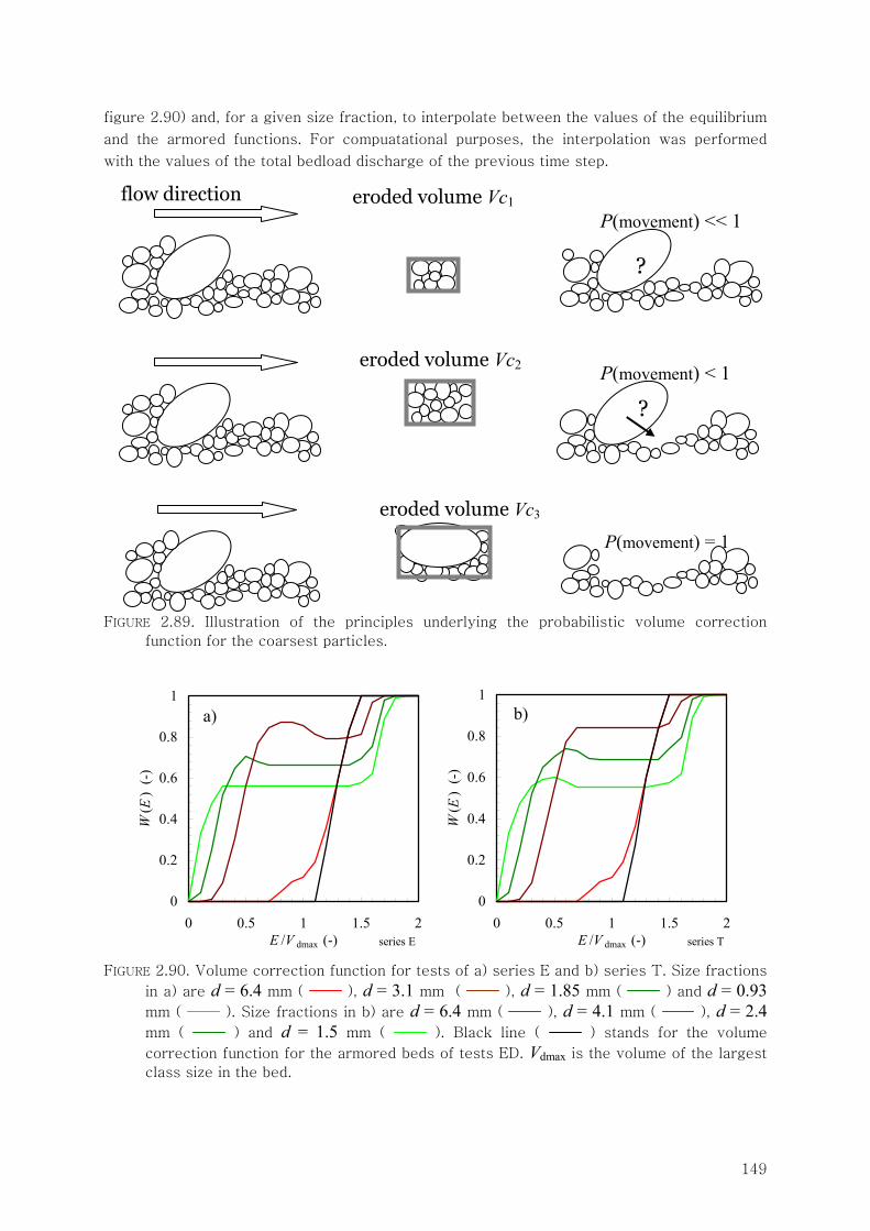
149

figure 2.90) and, for a given size fraction, to interpolate between the values of the equilibrium

and the armored functions. For compuatational purposes, the interpolation was performed

with the values of the total bedload discharge of the previous time step.

FIGURE 2.89. Illustration of the principles underlying the probabilistic volume correction

function for the coarsest particles.

0

0.2

0.4

0.6

0.8

1

0 0.5 1 1.5 2E /V dmax (-)

W(E

) (-

)

series E

0

0.2

0.4

0.6

0.8

1

0 0.5 1 1.5 2E /V dmax (-)

W(E

) (-

)

series T

FIGURE 2.90. Volume correction function for tests of a) series E and b) series T. Size fractions

in a) are d = 6.4 mm ( ), d = 3.1 mm ( ), d = 1.85 mm ( ) and d = 0.93

mm ( ). Size fractions in b) are d = 6.4 mm ( ), d = 4.1 mm ( ), d = 2.4

mm ( ) and d = 1.5 mm ( ). Black line ( ) stands for the volume

correction function for the armored beds of tests ED. Vdmax is the volume of the largest

class size in the bed.

eroded volume Vc1

?

flow direction

P(movement) << 1

?

eroded volume Vc2 P(movement) < 1

eroded volume Vc3

P(movement) = 1

a) b)

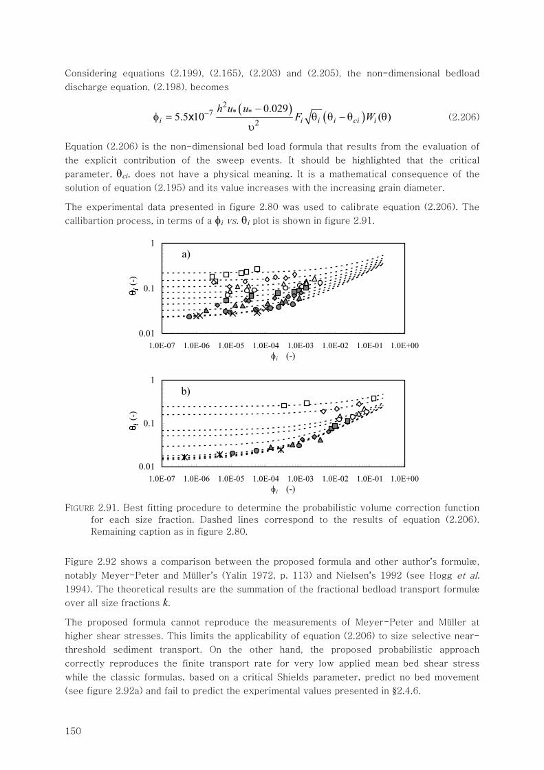
150

Considering equations (2.199), (2.165), (2.203) and (2.205), the non-dimensional bedload

discharge equation, (2.198), becomes

( ) ( )

2* *7

2

0.0295.5 10 ( )i i i i ci i

h u uF W− −

φ = θ θ − θ θυ

x (2.206)

Equation (2.206) is the non-dimensional bed load formula that results from the evaluation of

the explicit contribution of the sweep events. It should be highlighted that the critical

parameter, θci, does not have a physical meaning. It is a mathematical consequence of the

solution of equation (2.195) and its value increases with the increasing grain diameter.

The experimental data presented in figure 2.80 was used to calibrate equation (2.206). The

callibartion process, in terms of a φi vs. θi plot is shown in figure 2.91.

0.01

0.1

1

1.0E-07 1.0E-06 1.0E-05 1.0E-04 1.0E-03 1.0E-02 1.0E-01 1.0E+00φi (-)

i (-

)

0.01

0.1

1

1.0E-07 1.0E-06 1.0E-05 1.0E-04 1.0E-03 1.0E-02 1.0E-01 1.0E+00φi (-)

i (-

)

FIGURE 2.91. Best fitting procedure to determine the probabilistic volume correction function

for each size fraction. Dashed lines correspond to the results of equation (2.206).

Remaining caption as in figure 2.80.

Figure 2.92 shows a comparison between the proposed formula and other author’s formulæ,

notably Meyer-Peter and Müller’s (Yalin 1972, p. 113) and Nielsen’s 1992 (see Hogg et al.

1994). The theoretical results are the summation of the fractional bedload transport formulæ

over all size fractions k.

The proposed formula cannot reproduce the measurements of Meyer-Peter and Müller at

higher shear stresses. This limits the applicability of equation (2.206) to size selective near-

threshold sediment transport. On the other hand, the proposed probabilistic approach

correctly reproduces the finite transport rate for very low applied mean bed shear stress

while the classic formulas, based on a critical Shields parameter, predict no bed movement

(see figure 2.92a) and fail to predict the experimental values presented in §2.4.6.

a)

b)

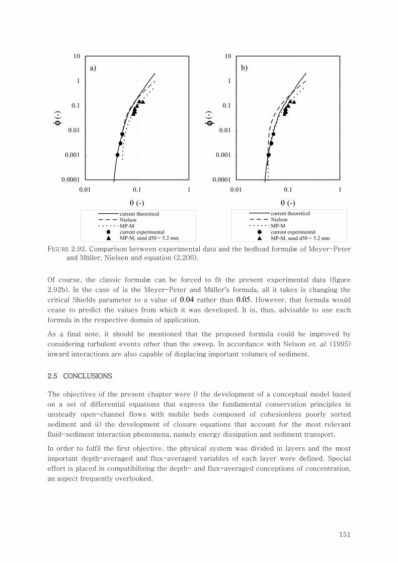
151

0.0001

0.001

0.01

0.1

1

10

0.01 0.1 1

θ (-)

∠ (-

)

current theoreticalNielsonMP-Mcurrent experimentalMP-M, sand d50 = 5.2 mm

0.0001

0.001

0.01

0.1

1

10

0.01 0.1 1

θ (-)∠

(-)

current theoreticalNielsonMP-Mcurrent experimentalMP-M, sand d50 = 5.2 mm

FIGURE 2.92. Comparison between experimental data and the bedload formulæ of Meyer-Peter

and Müller, Nielsen and equation (2.206).

Of course, the classic formulæ can be forced to fit the present experimental data (figure

2.92b). In the case of is the Meyer-Peter and Müller’s formula, all it takes is changing the

critical Shields parameter to a value of 0.04 rather than 0.05. However, that formula would

cease to predict the values from which it was developed. It is, thus, advisable to use each

formula in the respective domain of application.

As a final note, it should be mentioned that the proposed formula could be improved by

considering turbulent events other than the sweep. In accordance with Nelson et. al. (1995)

inward interactions are also capable of displacing important volumes of sediment.

2.5 CONCLUSIONS

The objectives of the present chapter were i) the development of a conceptual model based

on a set of differential equations that express the fundamental conservation principles in

unsteady open-channel flows with mobile beds composed of cohesionless poorly sorted

sediment and ii) the development of closure equations that account for the most relevant

fluid-sediment interaction phenomena, namely energy dissipation and sediment transport.

In order to fulfil the first objective, the physical system was divided in layers and the most

important depth-averaged and flux-averaged variables of each layer were defined. Special

effort is placed in compatibilizing the depth- and flux-averaged conceptions of concentration,

an aspect frequently overlooked.

a) b)

152

The conservation equations for each layer were developed by means of the application of

Reynolds’ transport theorem within the framework of the control volume technique. A

particular attention is given to the equation of mass conservation of the mixing layer.

The closure equations were derived for the class of flows for which the macroscopic flow

variables such as the friction slope and the sediment discharge are a result from the

integration of processes that take place at the scale of the grain. In particular, the bedload

formula, equation (2.206), is based on the quantification of the momentum transfer from the

fluid flow to the sediment grains, during the bursting cycle event called “sweep”. Bed-form

induced flow resistance was not studied nor any other aspects pertaining bed-form formation

and destruction.

The application of the model is thus limited flows that do not develop bed forms and for which

the sediment transport is size selective and near-threshold. This represents a large class of

open-channel flows, namely those with gravel and coarse sand beds subjected to low Froude

numbers.

The closure model, i.e., the set of semi-empirical or theoretical formulæ required to close the

system of conservation laws, was based on experimental data, either other researchers’ or

produced for that matter. The characterization of the velocity and shear-stress profiles,

turbulent intensities and higher order moments was performed for mobile and immobile bed

flows. The mean velocity of the particles in the bedload layer was also measured. This

allowed for the specification of the mean velocity in the bedload layer. The thickness of the

layers was devised mostly based on other authors’ data.

Total and fractional bedload discharges were experimentally measured for two sand and

gravel mixtures. The results were utilised to discuss unequal mobility of the size fractions,

notably hiding and protrusion effects, and to calibrate the bedload discharge formula. The

later is an event-driven bedload discharge formula which, for its development was necessary,

as mentioned above, to quantify the momentum associated to the sweep events.

In the process characterizing the turbulent bursting cycle, a number of fundamental

interrogations about the nature of the interaction between turbulent flows and bedload

transport arose. Do these flows have the same turbulent structures and follow the same

scaling laws as the flows over fixed beds? Are there important feedback mechanisms between

the organization of turbulence and the quality and quantity of the sediments moving in the

bed? If so, can we observe the echoes of such interactions on macroscopic parameters such

as the mean bed shear stress?

It was concluded that organised turbulence in flows with mobile beds is essentially identical

to that observed in immobile bed flows. However, it appears that some feedback occurs,

invisible in the mean variables and in the second-order moments but observable in the third-

order moments and related quantities: the flux of turbulent kinetic energy and the magnitude

of the maximum shear stress associated to sweep events in the roughness sub-layer.

A possibly related phenomenon is the increased grain mobility of the largest grains in the

presence moving finer fractions. This phenomenon was addressed empirically, by means of a

probabilistic correction to the volume of entrained particles. This, it is necessary that a

thorough experimental study aimed at the quantification of the feedback mechanisms between

near-bed sediment transport and organised turbulence is performed.

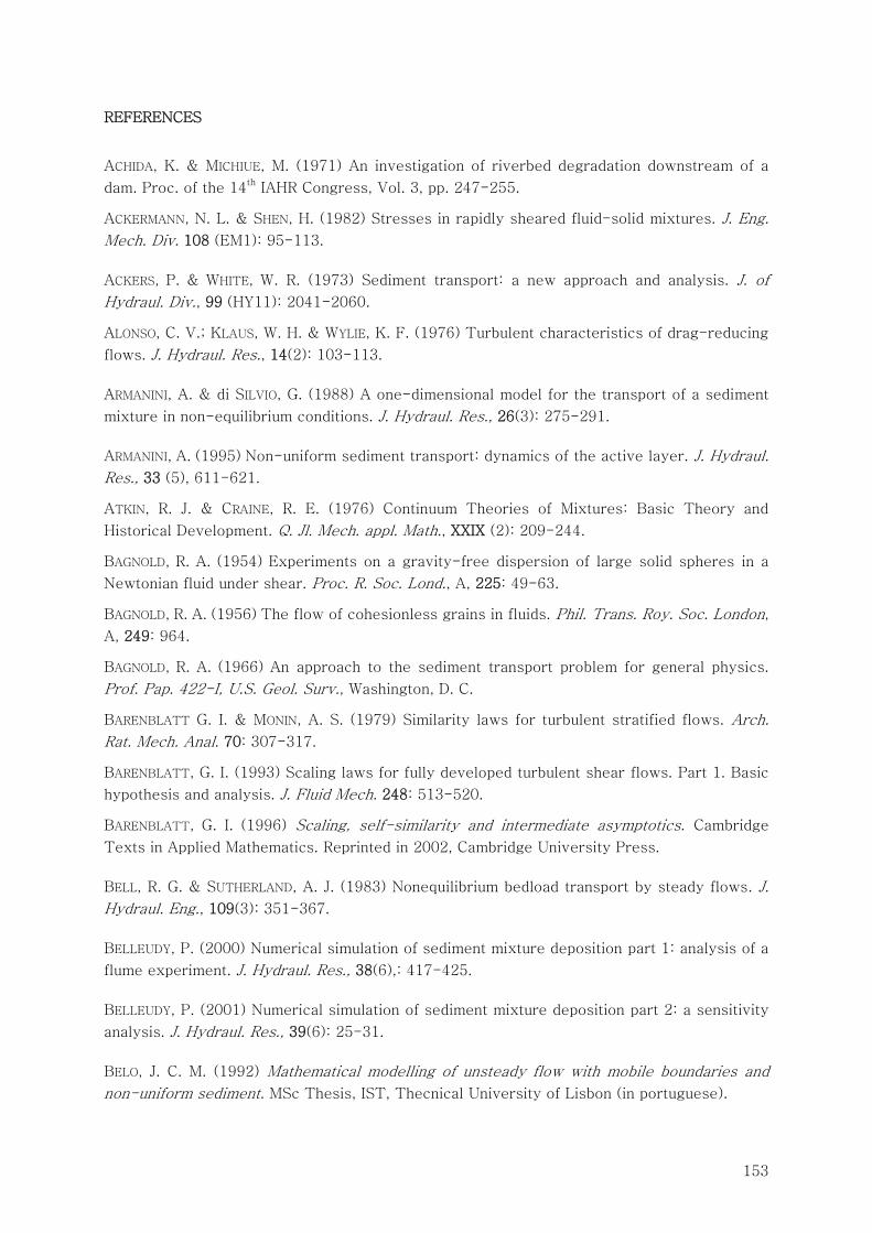
153

REFERENCES

ACHIDA, K. & MICHIUE, M. (1971) An investigation of riverbed degradation downstream of a

dam. Proc. of the 14th IAHR Congress, Vol. 3, pp. 247-255.

ACKERMANN, N. L. & SHEN, H. (1982) Stresses in rapidly sheared fluid-solid mixtures. J. Eng.

Mech. Div. 108 (EM1): 95-113.

ACKERS, P. & WHITE, W. R. (1973) Sediment transport: a new approach and analysis. J. of

Hydraul. Div., 99 (HY11): 2041-2060.

ALONSO, C. V.; KLAUS, W. H. & WYLIE, K. F. (1976) Turbulent characteristics of drag-reducing

flows. J. Hydraul. Res., 14(2): 103-113.

ARMANINI, A. & di SILVIO, G. (1988) A one-dimensional model for the transport of a sediment

mixture in non-equilibrium conditions. J. Hydraul. Res., 26(3): 275-291.

ARMANINI, A. (1995) Non-uniform sediment transport: dynamics of the active layer. J. Hydraul.

Res., 33 (5), 611-621.

ATKIN, R. J. & CRAINE, R. E. (1976) Continuum Theories of Mixtures: Basic Theory and

Historical Development. Q. Jl. Mech. appl. Math., XXIX (2): 209-244.

BAGNOLD, R. A. (1954) Experiments on a gravity-free dispersion of large solid spheres in a

Newtonian fluid under shear. Proc. R. Soc. Lond., A, 225: 49-63.

BAGNOLD, R. A. (1956) The flow of cohesionless grains in fluids. Phil. Trans. Roy. Soc. London,

A, 249: 964.

BAGNOLD, R. A. (1966) An approach to the sediment transport problem for general physics.

Prof. Pap. 422-I, U.S. Geol. Surv., Washington, D. C.

BARENBLATT G. I. & MONIN, A. S. (1979) Similarity laws for turbulent stratified flows. Arch.

Rat. Mech. Anal. 70: 307-317.

BARENBLATT, G. I. (1993) Scaling laws for fully developed turbulent shear flows. Part 1. Basic

hypothesis and analysis. J. Fluid Mech. 248: 513-520.

BARENBLATT, G. I. (1996) Scaling, self-similarity and intermediate asymptotics. Cambridge

Texts in Applied Mathematics. Reprinted in 2002, Cambridge University Press.

BELL, R. G. & SUTHERLAND, A. J. (1983) Nonequilibrium bedload transport by steady flows. J.

Hydraul. Eng., 109(3): 351-367.

BELLEUDY, P. (2000) Numerical simulation of sediment mixture deposition part 1: analysis of a

flume experiment. J. Hydraul. Res., 38(6),: 417-425.

BELLEUDY, P. (2001) Numerical simulation of sediment mixture deposition part 2: a sensitivity

analysis. J. Hydraul. Res., 39(6): 25-31.

BELO, J. C. M. (1992) Mathematical modelling of unsteady flow with mobile boundaries and

non-uniform sediment. MSc Thesis, IST, Thecnical University of Lisbon (in portuguese).

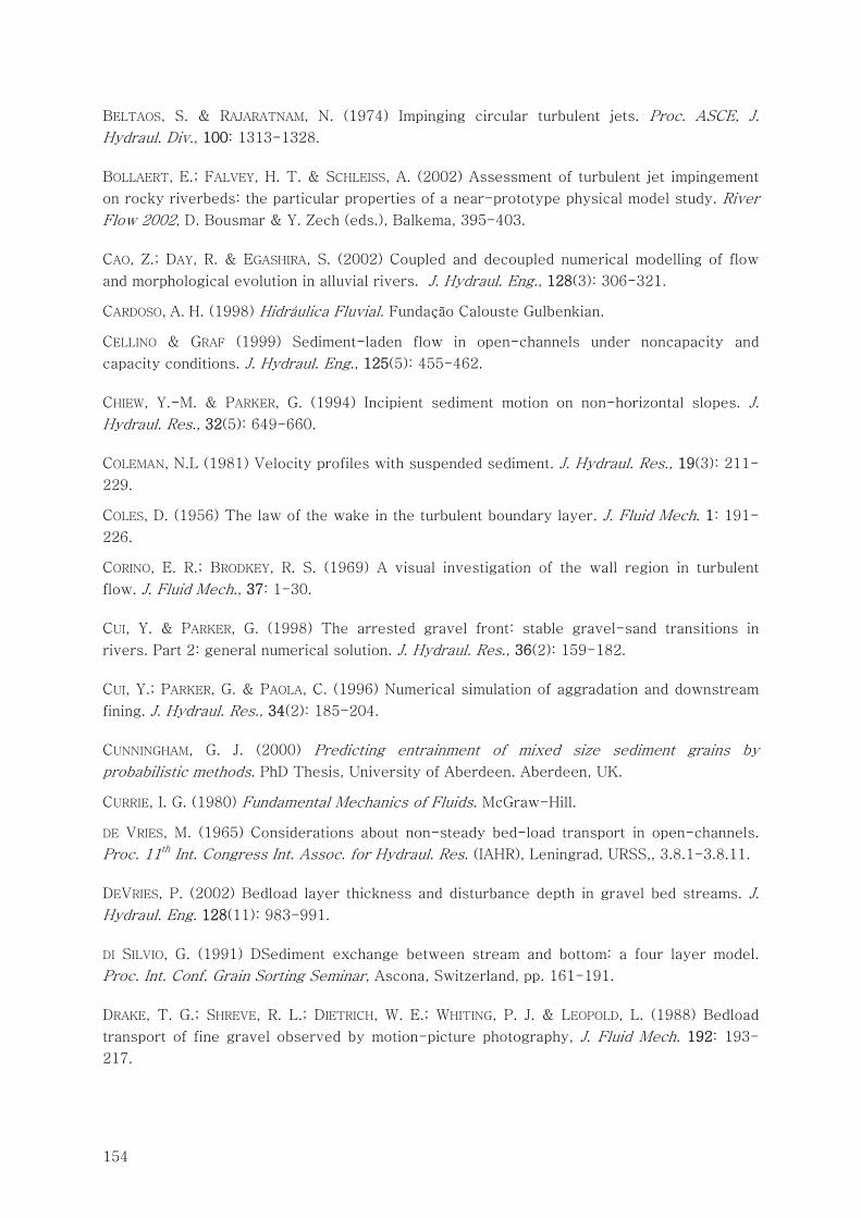
154

BELTAOS, S. & RAJARATNAM, N. (1974) Impinging circular turbulent jets. Proc. ASCE, J.

Hydraul. Div., 100: 1313-1328.

BOLLAERT, E.; FALVEY, H. T. & SCHLEISS, A. (2002) Assessment of turbulent jet impingement

on rocky riverbeds: the particular properties of a near-prototype physical model study. River

Flow 2002, D. Bousmar & Y. Zech (eds.), Balkema, 395-403.

CAO, Z.; DAY, R. & EGASHIRA, S. (2002) Coupled and decoupled numerical modelling of flow

and morphological evolution in alluvial rivers. J. Hydraul. Eng., 128(3): 306-321.

CARDOSO, A. H. (1998) Hidráulica Fluvial. Fundação Calouste Gulbenkian.

CELLINO & GRAF (1999) Sediment-laden flow in open-channels under noncapacity and

capacity conditions. J. Hydraul. Eng., 125(5): 455-462.

CHIEW, Y.-M. & PARKER, G. (1994) Incipient sediment motion on non-horizontal slopes. J.

Hydraul. Res., 32(5): 649-660.

COLEMAN, N.L (1981) Velocity profiles with suspended sediment. J. Hydraul. Res., 19(3): 211-

229.

COLES, D. (1956) The law of the wake in the turbulent boundary layer. J. Fluid Mech. 1: 191-

226.

CORINO, E. R.; BRODKEY, R. S. (1969) A visual investigation of the wall region in turbulent

flow. J. Fluid Mech., 37: 1-30.

CUI, Y. & PARKER, G. (1998) The arrested gravel front: stable gravel-sand transitions in

rivers. Part 2: general numerical solution. J. Hydraul. Res., 36(2): 159-182.

CUI, Y.; PARKER, G. & PAOLA, C. (1996) Numerical simulation of aggradation and downstream

fining. J. Hydraul. Res., 34(2): 185-204.

CUNNINGHAM, G. J. (2000) Predicting entrainment of mixed size sediment grains by

probabilistic methods. PhD Thesis, University of Aberdeen. Aberdeen, UK.

CURRIE, I. G. (1980) Fundamental Mechanics of Fluids. McGraw-Hill.

DE VRIES, M. (1965) Considerations about non-steady bed-load transport in open-channels.

Proc. 11th Int. Congress Int. Assoc. for Hydraul. Res. (IAHR), Leningrad, URSS,, 3.8.1-3.8.11.

DEVRIES, P. (2002) Bedload layer thickness and disturbance depth in gravel bed streams. J.

Hydraul. Eng. 128(11): 983-991.

DI SILVIO, G. (1991) DSediment exchange between stream and bottom: a four layer model.

Proc. Int. Conf. Grain Sorting Seminar, Ascona, Switzerland, pp. 161-191.

DRAKE, T. G.; SHREVE, R. L.; DIETRICH, W. E.; WHITING, P. J. & LEOPOLD, L. (1988) Bedload

transport of fine gravel observed by motion-picture photography, J. Fluid Mech. 192: 193-

217.

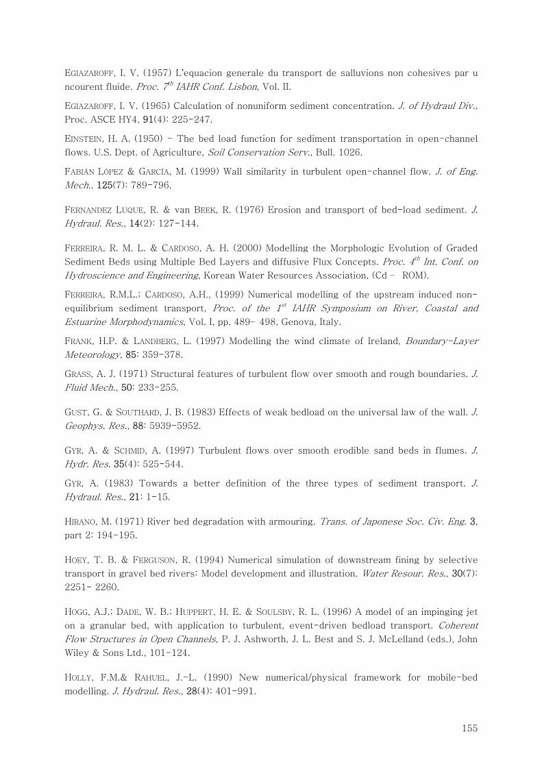
155

EGIAZAROFF, I. V. (1957) L’equacion generale du transport de salluvions non cohesives par u

ncourent fluide. Proc. 7th IAHR Conf. Lisbon, Vol. II.

EGIAZAROFF, I. V. (1965) Calculation of nonuniform sediment concentration. J. of Hydraul Div.,

Proc. ASCE HY4, 91(4): 225-247.

EINSTEIN, H. A. (1950) - The bed load function for sediment transportation in open-channel

flows. U.S. Dept. of Agriculture, Soil Conservation Serv., Bull. 1026.

FABIÁN LÓPEZ & GARCÍA, M. (1999) Wall similarity in turbulent open-channel flow. J. of Eng.

Mech., 125(7): 789-796.

FERNANDEZ LUQUE, R. & van BEEK, R. (1976) Erosion and transport of bed-load sediment. J.

Hydraul. Res., 14(2): 127-144.

FERREIRA, R. M. L. & CARDOSO, A. H. (2000) Modelling the Morphologic Evolution of Graded

Sediment Beds using Multiple Bed Layers and diffusive Flux Concepts. Proc. 4th Int. Conf. on

Hydroscience and Engineering, Korean Water Resources Association, (Cd – ROM).

FERREIRA, R.M.L.; CARDOSO, A.H., (1999) Numerical modelling of the upstream induced non-

equilibrium sediment transport, Proc. of the 1st IAHR Symposium on River, Coastal and

Estuarine Morphodynamics, Vol. I, pp. 489– 498, Genova, Italy.

FRANK, H.P. & LANDBERG, L. (1997) Modelling the wind climate of Ireland, Boundary-Layer

Meteorology, 85: 359-378.

GRASS, A. J. (1971) Structural features of turbulent flow over smooth and rough boundaries. J.

Fluid Mech., 50: 233-255.

GUST, G. & SOUTHARD, J. B. (1983) Effects of weak bedload on the universal law of the wall. J.

Geophys. Res., 88: 5939-5952.

GYR, A. & SCHMID, A. (1997) Turbulent flows over smooth erodible sand beds in flumes. J.

Hydr. Res. 35(4): 525-544.

GYR, A. (1983) Towards a better definition of the three types of sediment transport. J.

Hydraul. Res., 21: 1-15.

HIRANO, M. (1971) River bed degradation with armouring. Trans. of Japonese Soc. Civ. Eng. 3,

part 2: 194-195.

HOEY, T. B. & FERGUSON, R. (1994) Numerical simulation of downstream fining by selective

transport in gravel bed rivers: Model development and illustration. Water Resour. Res., 30(7):

2251- 2260.

HOGG, A.J.; DADE, W. B.; HUPPERT, H. E. & SOULSBY, R. L. (1996) A model of an impinging jet

on a granular bed, with application to turbulent, event-driven bedload transport. Coherent

Flow Structures in Open Channels, P. J. Ashworth, J. L. Best and S. J. McLelland (eds.), John

Wiley & Sons Ltd., 101-124.

HOLLY, F.M.& RAHUEL, J.-L. (1990) New numerical/physical framework for mobile-bed

modelling. J. Hydraul. Res., 28(4): 401-991.

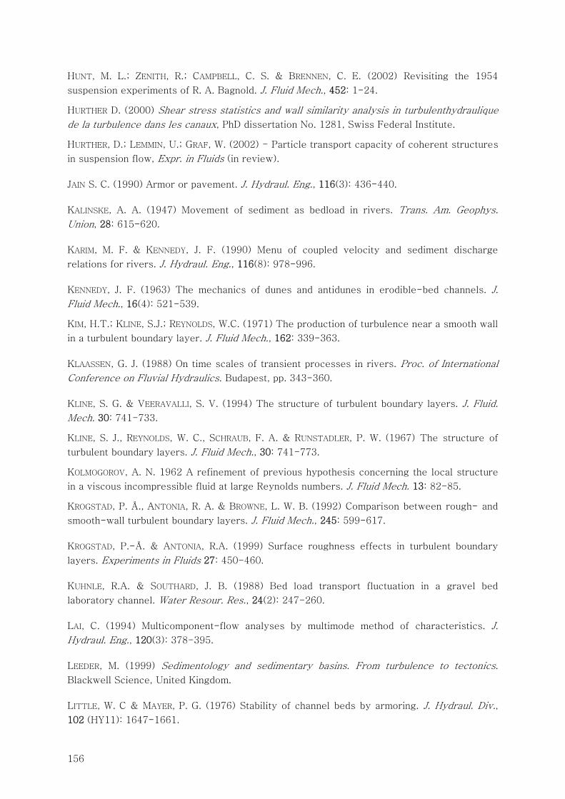
156

HUNT, M. L.; ZENITH, R.; CAMPBELL, C. S. & BRENNEN, C. E. (2002) Revisiting the 1954

suspension experiments of R. A. Bagnold. J. Fluid Mech., 452: 1-24.

HURTHER D. (2000) Shear stress statistics and wall similarity analysis in turbulenthydraulique

de la turbulence dans les canaux, PhD dissertation No. 1281, Swiss Federal Institute.

HURTHER, D.; LEMMIN, U.; GRAF, W. (2002) - Particle transport capacity of coherent structures

in suspension flow, Expr. in Fluids (in review).

JAIN S. C. (1990) Armor or pavement. J. Hydraul. Eng., 116(3): 436-440.

KALINSKE, A. A. (1947) Movement of sediment as bedload in rivers. Trans. Am. Geophys.

Union, 28: 615-620.

KARIM, M. F. & KENNEDY, J. F. (1990) Menu of coupled velocity and sediment discharge

relations for rivers. J. Hydraul. Eng., 116(8): 978-996.

KENNEDY, J. F. (1963) The mechanics of dunes and antidunes in erodible-bed channels. J.

Fluid Mech., 16(4): 521-539.

KIM, H.T.; KLINE, S.J.; REYNOLDS, W.C. (1971) The production of turbulence near a smooth wall

in a turbulent boundary layer. J. Fluid Mech., 162: 339-363.

KLAASSEN, G. J. (1988) On time scales of transient processes in rivers. Proc. of International

Conference on Fluvial Hydraulics. Budapest, pp. 343-360.

KLINE, S. G. & VEERAVALLI, S. V. (1994) The structure of turbulent boundary layers. J. Fluid.

Mech. 30: 741-733.

KLINE, S. J., REYNOLDS, W. C., SCHRAUB, F. A. & RUNSTADLER, P. W. (1967) The structure of

turbulent boundary layers. J. Fluid Mech., 30: 741-773.

KOLMOGOROV, A. N. 1962 A refinement of previous hypothesis concerning the local structure

in a viscous incompressible fluid at large Reynolds numbers. J. Fluid Mech. 13: 82-85.

KROGSTAD, P. Å., ANTONIA, R. A. & BROWNE, L. W. B. (1992) Comparison between rough- and

smooth-wall turbulent boundary layers. J. Fluid Mech., 245: 599-617.

KROGSTAD, P.-Å. & ANTONIA, R.A. (1999) Surface roughness effects in turbulent boundary

layers. Experiments in Fluids 27: 450-460.

KUHNLE, R.A. & SOUTHARD, J. B. (1988) Bed load transport fluctuation in a gravel bed

laboratory channel. Water Resour. Res., 24(2): 247-260.

LAI, C. (1994) Multicomponent-flow analyses by multimode method of characteristics. J.

Hydraul. Eng., 120(3): 378-395.

LEEDER, M. (1999) Sedimentology and sedimentary basins. From turbulence to tectonics.

Blackwell Science, United Kingdom.

LITTLE, W. C & MAYER, P. G. (1976) Stability of channel beds by armoring. J. Hydraul. Div.,

102 (HY11): 1647-1661.

157

LYN, D. A. & ALTINAKAR, M. (2002) St. Venant-Exner equations for near-critical and

transcritical flows. J. Hydraul. Eng., 128(6): 579-587.

LYN, D. A. & GOODWIN, P. (1987) Stability of a general Preissman Scheme. J. Hydraul. Eng.,

113(1): 16-27.

MACAULEY, A.N. & PENDER, G. (1999) The response of an armoured bed to the infiltration of

fine sand in a compound channel. Proc. 1st IAHR Symposium on River, Coastal and Estuarine

Morphodynamics, Genova, 6-10 September, pp. 141-149.

MAGALHÃES, L. T. (1993) Integrais em variedades e aplicações. Texto Editora.

MONIN, A. S. & YAGLOM, A. M. (1975) Statistical fluid mechanics. Vol. 2: Mechanics of

turbulence. MIT Press.

NAKAGAWA, H. & NEZU, I. (1977) Prediction of the contribution to the Reynolds stress from

bursting events in open-channel-flows. J. Fluid Mech. 80(1): 99-128.

NELSON, J. M, SHREVE, R. L., MCLEAN, S. R. & DRAKE, T. G. (1995) Role of near-bed turbulence

in bedload transport and bedform mechanics. Water Resour. Res., 31: 2071-2086.

NEZU, I. & NAKAGAWA, H. (1993) Turbulence in Open-Channel Flows. International Association

for Hydraulic Research, Monograph Series. Balkema, Rotterdam.

NIKORA, V. & GORING, D. (2000) Flow turbulence over fixed and weakly mobile gravel beds. J.

Hydr. Eng., 126(9): 679-690.

NIKORA, V., GORING, D., MCEWAN, I. & GRIFFITHS, G. (2001) Spatially averaged open-channel

flow over rough. J. Hydraul. Eng. 127(2): 123-133.

NIKORA, V; HABERSACK, H; HUBER, T & MCEWAN, I. (2002) On bed particle diffusion in gravel

bed flows under weak bed load transport. Water Resour. Res., 38(6).17: 1-9.

NIÑO, Y. & GARCIA, M. (1994) Gravel saltation, 2. Modelling. Water Resour. Res., 30(6): 1915-

1924

NIÑO, Y.; GARCIA, M. & AYALA, L. (1994) Gravel Saltation, 1. Experiments. Water Resour.

Res., 30(6): 1907-1914.

NIÑO, Y.; FABIAN LOPEZ & GARCIA, M. (2003) Threshold for particle entrainment into

suspension. Sedimentology 50: 247-263.

NIÑO, Y.; GARCIA, M. H. (1996) Experiments on particle-turbulence interactions in the near-

wall region of an open channel flow: implications for sediment transport. J. Fluid Mech., 326:

285-319.

PARKER, G. & CUI, Y. (1998) The arrested gravel front: stable gravel-sand transitions in

rivers. Part 1: simplified analytical solution. J. Hydraul. Res., 36(1): 75-100.

PARKER, G. & SUTHERLAND (1990) Fluvial armor. J. Hydraul. Res., 28(5): 529-543.

158

PARKER, G. (1990) Surface-based bedload transport relation for gravel rivers. J. Hydraul.

Res., 28(4): 417-436.

PARKER, G. (1991) Selective sorting and abrasion of river gravel. I: Theory. J. Hydraul. Eng.,

117(2): 131-149.

PARKER, G.; KLINGEMAN, P.C. & McLEAN, D.G. (1982) Bedload and size distribution in paved

gravel-bed streams. J. Hydraul. Div. 108(HY4): 544-571.

PARKER, G.; PAOLA, C. & LECLAIR, S. (2000) Probabilistic Exner sediment continuity equation

for mixtures with no active layer, J. Hydraul. Eng., 126(11): 818 - 826.

PARKER, G.; SEMINARA, G. & SOLARI, L. (2003) Bed load at low shields stress on arbitrarily

sloping beds: alternative entrainment formulation. Water Resour. Res., 39(7).2: 1-11.

PERRY, A. E., W. H. SCHOFIELD, & P. N. JOUBERT (1969) Rough wall turbulent boundary layers.

J. Fluid Mech. 37: 383-413.

PHILLIPS, B. & SUTHERLAND, A. (1989) Spatial lag effects in bed load sediment transport. J.

Hydraul. Res. 27(1): 115- 133.

POPE, S. B. (2000) Turbulent flows. Cambridge University Press.

PREISSMANN, A. (1961) Propagation des intumescences dans les canaux et les rivìeres. Actes

du 1er Congrès de l’ Assocaition Francaise de Calcul, Grenoble, pp. 433-442.

RAHUEL, J. L.; HOLLY, F. M.; CHOLLET, J. P., BELLEUDY, P. J. & YANG, G. (1989) Modeling of

riverbed evolution for bedload sediment mixtures. J. Hydraul. Eng., 115(11): 1521-1542.

RAUPACH, M. R., R. A. ANTONIA, and S. RAJAGOPALAN (1991) Rough-wall turbulent boundary

layers. Appl. Mech. Review 44(1): 1-25.

RIBBERINK, J. S. (1987) Mathematical modelling of one-dimensional morphological changes in

rivers with non-uniform sediment. Communications on hydraulic and geotechinical

engineering. Faculty of Civil Engineering. Delft University of Technology.

ROLLAND, T. & LEMMIN, U. (1997) A two-component acoustic velocity profiler for use in

turbulent open-channel flow. J. Hydr. Res. 33(4): 545-561.

SADDOUGHI, S. G. & VEERAVALLI, S. V. (1994) Local isotropy in turbulent boundary layers at

high Reynolds number. J. Fluid. Mech. 268: 333-372.

SAIEDI, S. (1997) Coupled modelling of alluvial flows. J. Hydraul. Eng., 123(5): 440-446.

SCHMEECKLE, M. W. & NELSON, J. M. (2003) Direct numerical simulation of bedload transport

using a local, dynamic boundary condition. Sedimentology 50: 279-301.

SECHET, P. & Le GUENNEC, B. (1999) Bursting phenomenon and incipient motion of solid

particles in bed-load transport. J. Hydraul. Res., 37(5): 683-696.

159

SEMINARA, G.; COLOMBINI, M. & PARKER, G.; (1996) Nearly pure sorting waves and formation of

bedload sheets. J. Hydraul. Res., 312(3): 253-278.

SEMINARA, G.; SOLARI, L. & PARKER, G. (2002) Bed load at low Shields stress on arbitrary

sloping beds: failure of the Bagnold hypothesis. Water Resour. Res., 38(11): 1249.

SIBANDA, E.; McEWAN, I. & MARION, A. (2000) Measuring the structure of mixed-grain-size

sediment beds J. Hydraul. Eng., 126(5): 1-7.

SIEBEN, J. (1999) A theoretical analysis of discontinuous flow with mobile bed. J. Hydraul.

Res., 37(2): 199-212.

SIEBEN, J. (1999) A theoretical analysis on armouring of river beds, J. Hydraul. Res., 37(3):

313-326.

SLOFF, C. J. (1993) Analysis of basic equations of sediment laden flows. Communications on

Hydraulic and Geotechnical Engineering, Rept. No 93-8, Delft Uneversity of Technology,

Delft, The Netherlands.

SMART, M. G. (1999) Turbulent Velocity Profiles and Boundary Shear in Gravel Bed Rivers. J.

Hydraul. Eng., 125(2): 106- 117.

SONG, T., GRAF, W. H. & LEMMIN, U. (1994) Uniform flow in open-channels with movable gravel

bed. J. Hydraul. Res., 32 (6): 861-876.

SUMER, B. M. & DEIGAARD, R. (1981) Particle motions near the bottom of in turbulent flow in an

open channel initial. J. Fluid Mech., 109: 311-337.

SUMER, B. M.; KOZAKIEWICZ, A.; FREDSØE, J. & DEIGARD, R. (1996) Velocity and Concentration

Profiles in Sheet-Flow Layer of Movable Bed. J. Hydraul. Eng. 122: 549-558.

SUTHERLAND, A. J. (1967) Proposed mechanism for sediment entrainment by turbulent flows. J.

Geophys. Res. 72(24): 6183-6193.

THOMAS, W. A. & PRASUHN, A. L. (1977) Mathematical modelling of scour and deposition.

J.Hydraul.Div. 103(HY8): 851-863.

TORO-ESCOBAR, C. M.; PARKER, G. & PAOLA, C. (1996) Transfer function for the deposition of

poorly sorted gravel in response to streambed aggradation. J. Hydraul. Res., 34(1): 35-53.

TOWNSEND, A. A. (1976) The Structure of Turbulent Shear Flows. 2nd edition, Cambridge Univ.

Press.

VAN DYKE, M. (1964) Perturbation methods in fluid mechanics. Academic Press.

VAN RIJN, L. C. (1987) Mathematical Modelling of Morphological Processes in the case of

Suspended Sediment Transport. Faculty of Civil Engineering. Delft University of Technology.

VAN RIJN, L. C. (1984) Sediment transport, Part I: bed load transport. J. Hydraul. Eng. 110(10):

1431-1456.

160

VOGEL, K. R.; van NIEKERK, A.; SLINGERLAND, R. L. & BRIDGE, J. S. (1992) Routing of

heterogeneous sediments over movable bed: model verification. J. Hydraul. Eng., 118(2):

263-279.

WEI, T. & WILLMARTH, W. W. (1992) Modifying turbulent structure with drag-reducing polymer

additives in turbulent channel flows. J. Fluid Mech., 245: 619-641.

WHITE, F. M. (1986) Fluid Mechanics. McGaw-Hill International Editions.

WHITE, W. R., Paris, E. & BETESS, R. (1979) A new general method for predicting the frictional

characteristics of alluvial streams. Report no. IT 187, HR Wallingford, Wallingford,

Oxfordshire, UK.

WILCOCK, P. R; KENWORTHY, S. & CROWE, J. (2001) Experimental study of the transport of

mixed sand and gravel. Water Resour. Res., 37(12): 3349-3358.

WILCOCK, P.R & McARDELL, B. W. (1997) Partial transport of a sand/gravel sediment. Water

Resour. Res., 33(1): 235-245.

WILCOCK, P.R; BARTA, A. F., SHEA, C. C.; KONDOLF, G. M.; MATTHEWS, W. V. & PITLICK, J.

(1996) Observations of flow and sediment entrainment on a large gravel-bed river. Water

Resour. Res., 32(9): 2897-2909.

WILLMARTH, W. W. & SHARMA, L. K. (1984) Study of turbulent structure with hot wires smaller

than the viscous length. J. Fluid Mech., 142: 121-149.

WILSON, K. C. (1987) Analysis of Bed-Load Motion at High Shear Stress. J. Hydraul. Eng. 113:

97-103.

WU, W.; WANG, S. S. Y. & JIA, Y. (2000) Nonuniform sediment transport in alluvial rivers. J.

Hydraul. Res., 38(6): 427-433.

YALIN, M. S. (1977) Mechanics of sediment transport. 2nd Edition, Pergamon Press.

YALIN, M. S. (1992) River Mechanics. Pergamon Press.

YANG, Y. & HIRANO, M. (1995) Discussion of: Uniform flow in open channels with movable

gravel bed, by T. Song, W. H. Graf and U. Lemmin, S. in J. Hidraul. Res., vol. 32 (1994) No. 6,

pp. 861-876. J. Hydraul. Res. 33(6): 877 – 880.

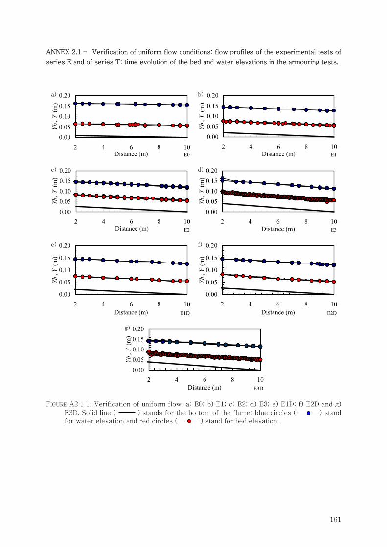
161

ANNEX 2.1 – Verification of uniform flow conditions: flow profiles of the experimental tests of

series E and of series T; time evolution of the bed and water elevations in the armouring tests.

0.000.050.100.150.20

2 4 6 8 10Distance (m)

Yb, Y

(m)

E0

a)

0.000.050.100.150.20

2 4 6 8 10Distance (m)

Yb, Y

(m)

E1

b)

0.000.050.100.150.20

2 4 6 8 10Distance (m)

Yb, Y

(m)

E2

c)

0.000.050.100.150.20

2 4 6 8 10Distance (m)

Yb, Y

(m)

E3

d)

0.00

0.05

0.10

0.15

0.20

2 4 6 8 10Distance (m)

Yb, Y

(m)

E1D

e)

0.00

0.05

0.10

0.15

0.20

2 4 6 8 10Distance (m)

Yb, Y

(m)

E2D

f)

0.000.050.100.150.20

2 4 6 8 10Distance (m)

Yb, Y

(m)

E3D

g)

FIGURE A2.1.1. Verification of uniform flow. a) E0; b) E1; c) E2; d) E3; e) E1D; f) E2D and g)

E3D. Solid line ( ) stands for the bottom of the flume; blue circles ( ) stand

for water elevation and red circles ( ) stand for bed elevation.

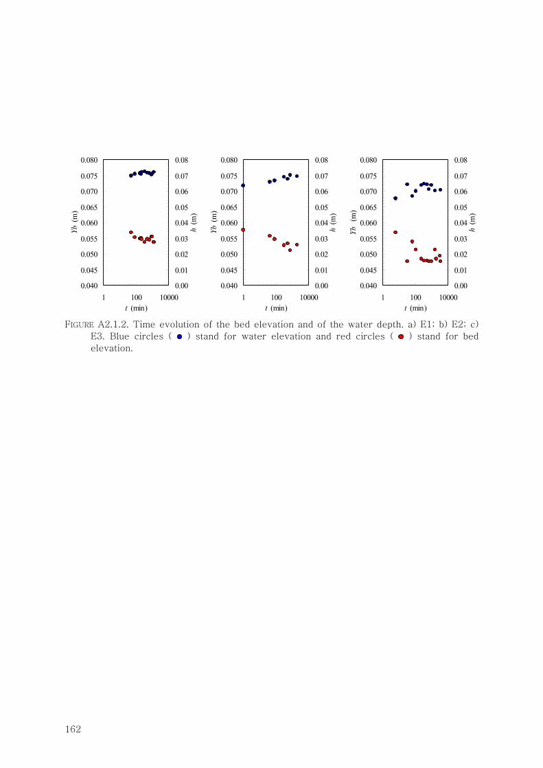
162

0.040

0.045

0.050

0.055

0.060

0.065

0.070

0.075

0.080

1 100 10000t (min)

Yb (m

)

0.00

0.01

0.02

0.03

0.04

0.05

0.06

0.07

0.08

h (m

)

0.040

0.045

0.050

0.055

0.060

0.065

0.070

0.075

0.080

1 100 10000t (min)

Yb (m

)

0.00

0.01

0.02

0.03

0.04

0.05

0.06

0.07

0.08

h (m

)

0.040

0.045

0.050

0.055

0.060

0.065

0.070

0.075

0.080

1 100 10000t (min)

Yb (

m)

0.00

0.01

0.02

0.03

0.04

0.05

0.06

0.07

0.08

h (m

)

FIGURE A2.1.2. Time evolution of the bed elevation and of the water depth. a) E1; b) E2; c)

E3. Blue circles ( ) stand for water elevation and red circles ( ) stand for bed

elevation.

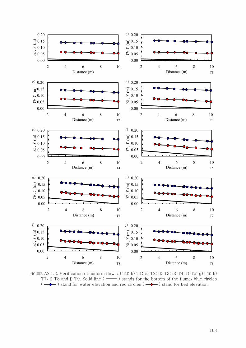
163

0.000.050.100.150.20

2 4 6 8 10Distance (m)

Yb, Y

(m)

0.000.050.100.150.20

2 4 6 8 10Distance (m)

Yb,Y

(m)

T1

b)

0.000.050.100.150.20

2 4 6 8 10Distance (m)

Yb,Y

(m)

T2

c)

0.000.050.100.150.20

2 4 6 8 10Distance (m)

Yb, Y

(m)

T3

d)

0.000.050.100.150.20

2 4 6 8 10Distance (m)

Yb, Y

(m)

T4

e)

0.000.050.100.150.20

2 4 6 8 10Distance (m)

Yb, Y

(m)

T5

f)

0.000.050.100.150.20

2 4 6 8 10Distance (m)

Yb, Y

(m)

T6

g)

0.000.050.100.150.20

2 4 6 8 10Distance (m)

Yb,Y

(m)

T7

h)

0.000.050.100.150.20

2 4 6 8 10Distance (m)

Yb, Y

(m)

T8

i)

0.000.050.100.150.20

2 4 6 8 10Distance (m)

Yb, Y

(m)

T9

j)

FIGURE A2.1.3. Verification of uniform flow. a) T0; b) T1; c) T2; d) T3; e) T4; f) T5; g) T6; h)

T7; i) T8 and j) T9. Solid line ( ) stands for the bottom of the flume; blue circles

( ) stand for water elevation and red circles ( ) stand for bed elevation.

164

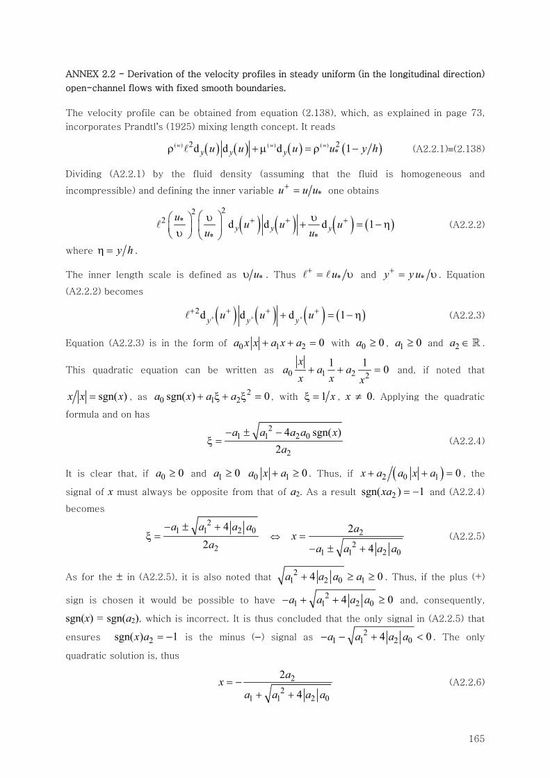
165

ANNEX 2.2 - Derivation of the velocity profiles in steady uniform (in the longitudinal direction)

open-channel flows with fixed smooth boundaries.

The velocity profile can be obtained from equation (2.138), which, as explained in page 73,

incorporates Prandtl’s (1925) mixing length concept. It reads

( ) ( ) ( ) ( )( ) ( ) ( )2 2*d d d 1w w w

y y yu u u u y hρ + μ = ρ − (A2.2.1)≡(2.138)

Dividing (A2.2.1) by the fluid density (assuming that the fluid is homogeneous and

incompressible) and defining the inner variable *u u u+ = one obtains

( ) ( ) ( ) ( )22

2 *

* *d d d 1y y y

uu u u

u u+ + +⎛ ⎞υ υ⎛ ⎞ + = − η⎜ ⎟⎜ ⎟υ⎝ ⎠ ⎝ ⎠

(A2.2.2)

where y hη = .

The inner length scale is defined as *uυ . Thus *u+ = υ and *y y u+ = υ . Equation

(A2.2.2) becomes

( ) ( ) ( ) ( )2d d d 1y y yu u u+ + ++ + + ++ = − η (A2.2.3)

Equation (A2.2.3) is in the form of 0 1 2 0a x x a x a+ + = with 0 0a ≥ , 1 0a ≥ and 2a ∈ .

This quadratic equation can be written as 0 1 2 21 1 0

xa a a

x x x+ + = and, if noted that

sgn( )x x x= , as 2

0 1 2sgn( ) 0a x a a+ ξ + ξ = , with 1 xξ = , x ≠ 0. Applying the quadratic

formula and on has

21 1 2 0

2

4 sgn( )2

a a a a xa

− ± −ξ = (A2.2.4)

It is clear that, if 0 0a ≥ and 1 0a ≥ 0 1 0a x a+ ≥ . Thus, if ( )2 0 1 0x a a x a+ + = , the

signal of x must always be opposite from that of a2. As a result 2sgn( ) 1xa = − and (A2.2.4)

becomes

21 1 2 0

2

42

a a a aa

− ± +ξ = ⇔ 2

21 1 2 0

2

4

ax

a a a a=

− ± + (A2.2.5)

As for the ± in (A2.2.5), it is also noted that 2

1 2 0 14 0a a a a+ ≥ ≥ . Thus, if the plus (+)

sign is chosen it would be possible to have 2

1 1 2 04 0a a a a− + + ≥ and, consequently,

sgn(x) = sgn(a2), which is incorrect. It is thus concluded that the only signal in (A2.2.5) that

ensures 2sgn( ) 1x a = − is the minus (−) signal as 2

1 1 2 04 0a a a a− − + < . The only

quadratic solution is, thus

22

1 1 2 0

2

4

ax

a a a a= −

+ + (A2.2.6)

166

It follows from (A2.2.6) that the solution of (A2.2.3) is

( ) ( )( )2

2 1d

1 1 4 1y u+

++

− η=

+ + − η (A2.2.7)

Far from the free surface region one has 1η and (A2.2.7) becomes

( )2

2d1 1 4

y u++

+=

+ + (A2.2.8)

Prandtl 1925 (see White 1986, p. 299) proposed a simple model for the mixing length: it

would increase almost linearly from the boundary, only dampened by a simple decaying law.

In inner variables, it reads

( )261 e yy++ + −= κ − (A2.2.9)

where the number 26 was determined experimentally by van Driest in 1956 (cf. Pope 2000, p.

304). Equation (A2.2.8) becomes

( )( ) 2

26

2d

1 1 4 1 ey

y

u

y+

+

+

+ −

=⎡ ⎤+ + κ −⎢ ⎥⎣ ⎦

(A2.2.10)

In the immediate vicinity of the boundary y+ << 1 and 26 1e y+− ≈ . Thus

( )d 1y u++ = (A2.2.11)

In the outer regions of the inner layer (logarithmic sublayer)

( )( ) ( )

( )

2 21 1 1 1

4 2

2 2d

4 4

1d

y

y yy y

y

u

y y

uy

+

+ ++ +

+

+

+ +κ κκ κ

≈ =

++

= =⎛ ⎞ ⎛ ⎞⎜ ⎟ ⎜ ⎟κ + + κ + +⎜ ⎟ ⎜ ⎟⎝ ⎠ ⎝ ⎠

=κ

(A2.2.12)

The solution of (A2.2.11), given the boundary condition at the wall, 0(0) 0u u+ += = , is

u y+ += (A2.2.13)

Equation (A2.2.13) is valid in the viscous sublayers and in most of the buffer sublayer. In the

logarithmic sublayer, the solution of (A2.2.12) is

( ) ( ) ( )

( )

1 1

1

1d ln ln

ln

a ay u u u y yy

u y B

++ + + + +

κ κ+

+ +κ

= ⇔ − = −κ

= +

(A2.2.14)

where ya lies in the logarithmic sublayer. Equation (A2.2.14), known as the log-law, is valid

also in the intermediate flow layer. As seen in §2.4.1, p. 73, it can also be derived from

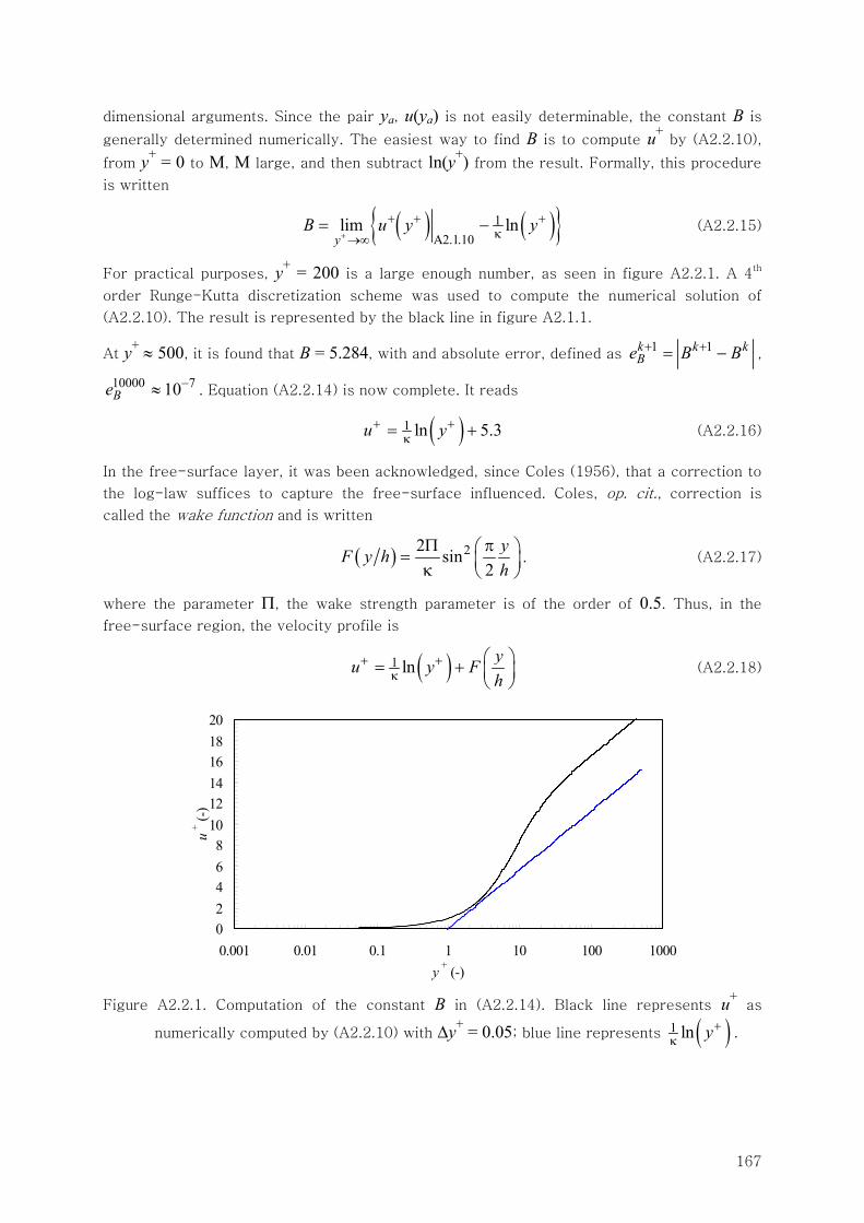
167

dimensional arguments. Since the pair ya, u(ya) is not easily determinable, the constant B is

generally determined numerically. The easiest way to find B is to compute u+ by (A2.2.10),

from y+ = 0 to M, M large, and then subtract ln(y+) from the result. Formally, this procedure

is written

( ) ( ){ }1A2.1.10

lim lny

B u y y+

+ + +κ→∞

= − (A2.2.15)

For practical purposes, y+ = 200 is a large enough number, as seen in figure A2.2.1. A 4th

order Runge-Kutta discretization scheme was used to compute the numerical solution of

(A2.2.10). The result is represented by the black line in figure A2.1.1.

At y+ ≈ 500, it is found that B = 5.284, with and absolute error, defined as 1 1k k k

Be B B+ += − ,

10000 710Be −≈ . Equation (A2.2.14) is now complete. It reads

( )1 ln 5.3u y+ +κ= + (A2.2.16)

In the free-surface layer, it was been acknowledged, since Coles (1956), that a correction to

the log-law suffices to capture the free-surface influenced. Coles, op. cit., correction is

called the wake function and is written

( ) 22 sin2

yF y hh

Π π⎛ ⎞= ⎜ ⎟κ ⎝ ⎠. (A2.2.17)

where the parameter Π, the wake strength parameter is of the order of 0.5. Thus, in the

free-surface region, the velocity profile is

( )1 ln yu y Fh

+ +κ

⎛ ⎞= + ⎜ ⎟⎝ ⎠

(A2.2.18)

02468

101214161820

0.001 0.01 0.1 1 10 100 1000y + (-)

u+ (-

)

Figure A2.2.1. Computation of the constant B in (A2.2.14). Black line represents u+ as

numerically computed by (A2.2.10) with Δy+ = 0.05; blue line represents ( )1 ln y+κ .

168

169

ANNEX 2.3 - Derivation of the sediment concentration in the bedload layer corresponding to

the formula of Meyer Peter & Müller (MP-M)

The cinematic concentration is an approximation of the static concentration. It is defined as

b sb bC q q≈ where qb is the total discharge in the bedload layer. Introducing the MP-M

formula and the definition of the total discharge qb in the definition, one has

( )

323( 1) 0.05s

bb b

b g s dC

u h− θ −

≈ (A2.3.1)

where 4 < b < 8 and where ub combines the sediment and fluid velocities in the following

manner

( )1b cb b wb bu u C u C= + − (A2.3.2)

For the sake of simplicity, the concentration will be considered constant. As a result, the

continuum velocity in the layer can be expressed by the simple formula 12( 1)b su b g s d= − θ .

In the same manner, the thickness of the bedload layer is considered constant, b sh ad= ,

1<a<4. Introducing these expressions in (A2.3.1) one has

( ) ( )

32 31

2212

31( 1) 0.05

0.05( 1)

sb a

s s

b g s dC

b g s d ad

−− θ −≈ = θ θ −

− θ (A2.3.3)

In order to express the concentration as a function of the Reynolds number, it is noted that

3 32 23 2 2

22

( 1) ( 1)10.05 0.05( 1) ( 1)

f fs sb

s sff s

C u C ub g s d g s dC

g s d a g s du Cb C u ad

⎛ ⎞ ⎛ ⎞− −⎜ ⎟ ⎜ ⎟= − = −⎜ ⎟ ⎜ ⎟− −⎝ ⎠ ⎝ ⎠

because ( )2 ( 1)f sC u g s dθ = − . The relevant Reynolds number is defined as

*Re f sb s s b C udu d bu d= = =

υ υ υ (A2.3.4)

It should be highlighted that, given the value of b, (A2.3.4) expresses a Reynolds number

approximately twice the value of *s sk k u+ = υ . The velocity is, thus

( )2 2 2 2 2Re s fu b d C= υ and the concentration becomes

32 2 2 2 2

2 2 2 2

33 2 2 2 2

2 2 2 3

( 1)1 Re 0.05( 1)Re

1 ( 1) Re 0.05Re ( 1)

s f fsb

f s s f

sb

s

b d C Cg s dC

a C g s d b d C

gd b sCa b s gd

⎛ ⎞− υ⎜ ⎟≈ −⎜ ⎟−υ ⎝ ⎠

⎛ ⎞− υ= −⎜ ⎟⎜ ⎟υ −⎝ ⎠

(A2.3.5)

170

Underlying this formula there is the relation between the Shields parameter and the Reynolds

number

2 2

2 3Re( 1) sb s gd

υθ =

−. (A2.3.6)

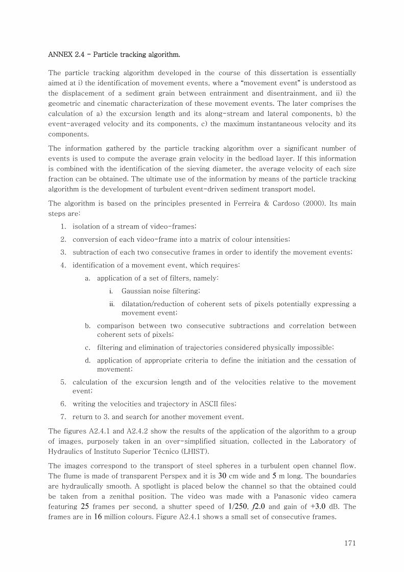
171

ANNEX 2.4 - Particle tracking algorithm.

The particle tracking algorithm developed in the course of this dissertation is essentially

aimed at i) the identification of movement events, where a “movement event” is understood as

the displacement of a sediment grain between entrainment and disentrainment, and ii) the

geometric and cinematic characterization of these movement events. The later comprises the

calculation of a) the excursion length and its along-stream and lateral components, b) the

event-averaged velocity and its components, c) the maximum instantaneous velocity and its

components.

The information gathered by the particle tracking algorithm over a significant number of

events is used to compute the average grain velocity in the bedload layer. If this information

is combined with the identification of the sieving diameter, the average velocity of each size

fraction can be obtained. The ultimate use of the information by means of the particle tracking

algorithm is the development of turbulent event-driven sediment transport model.

The algorithm is based on the principles presented in Ferreira & Cardoso (2000). Its main

steps are:

1. isolation of a stream of video-frames;

2. conversion of each video-frame into a matrix of colour intensities;

3. subtraction of each two consecutive frames in order to identify the movement events;

4. identification of a movement event, which requires:

a. application of a set of filters, namely:

i. Gaussian noise filtering;

ii. dilatation/reduction of coherent sets of pixels potentially expressing a

movement event;

b. comparison between two consecutive subtractions and correlation between

coherent sets of pixels;

c. filtering and elimination of trajectories considered physically impossible;

d. application of appropriate criteria to define the initiation and the cessation of

movement;

5. calculation of the excursion length and of the velocities relative to the movement

event;

6. writing the velocities and trajectory in ASCII files;

7. return to 3. and search for another movement event.

The figures A2.4.1 and A2.4.2 show the results of the application of the algorithm to a group

of images, purposely taken in an over-simplified situation, collected in the Laboratory of

Hydraulics of Instituto Superior Técnico (LHIST).

The images correspond to the transport of steel spheres in a turbulent open channel flow.

The flume is made of transparent Perspex and it is 30 cm wide and 5 m long. The boundaries

are hydraulically smooth. A spotlight is placed below the channel so that the obtained could

be taken from a zenithal position. The video was made with a Panasonic video camera

featuring 25 frames per second, a shutter speed of 1/250, f2.0 and gain of +3.0 dB. The

frames are in 16 million colours. Figure A2.4.1 shows a small set of consecutive frames.

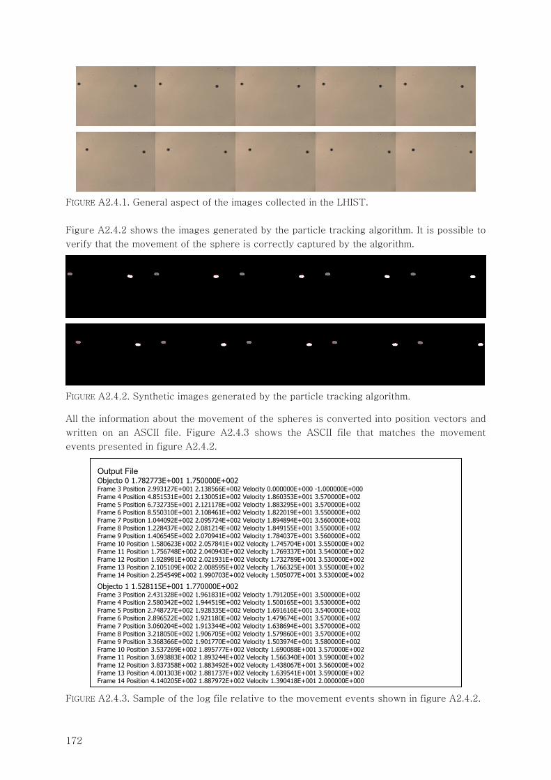
172

FIGURE A2.4.1. General aspect of the images collected in the LHIST.

Figure A2.4.2 shows the images generated by the particle tracking algorithm. It is possible to

verify that the movement of the sphere is correctly captured by the algorithm.

FIGURE A2.4.2. Synthetic images generated by the particle tracking algorithm.

All the information about the movement of the spheres is converted into position vectors and

written on an ASCII file. Figure A2.4.3 shows the ASCII file that matches the movement

events presented in figure A2.4.2.

FIGURE A2.4.3. Sample of the log file relative to the movement events shown in figure A2.4.2.

Output File Objecto 0 1.782773E+001 1.750000E+002 Frame 3 Position 2.993127E+001 2.138566E+002 Velocity 0.000000E+000 -1.000000E+000 Frame 4 Position 4.851531E+001 2.130051E+002 Velocity 1.860353E+001 3.570000E+002 Frame 5 Position 6.732735E+001 2.121178E+002 Velocity 1.883295E+001 3.570000E+002 Frame 6 Position 8.550310E+001 2.108461E+002 Velocity 1.822019E+001 3.550000E+002 Frame 7 Position 1.044092E+002 2.095724E+002 Velocity 1.894894E+001 3.560000E+002 Frame 8 Position 1.228437E+002 2.081214E+002 Velocity 1.849155E+001 3.550000E+002 Frame 9 Position 1.406545E+002 2.070941E+002 Velocity 1.784037E+001 3.560000E+002 Frame 10 Position 1.580623E+002 2.057841E+002 Velocity 1.745704E+001 3.550000E+002 Frame 11 Position 1.756748E+002 2.040943E+002 Velocity 1.769337E+001 3.540000E+002 Frame 12 Position 1.928981E+002 2.021931E+002 Velocity 1.732789E+001 3.530000E+002 Frame 13 Position 2.105109E+002 2.008595E+002 Velocity 1.766325E+001 3.550000E+002 Frame 14 Position 2.254549E+002 1.990703E+002 Velocity 1.505077E+001 3.530000E+002

Objecto 1 1.528115E+001 1.770000E+002 Frame 3 Position 2.431328E+002 1.961831E+002 Velocity 1.791205E+001 3.500000E+002 Frame 4 Position 2.580342E+002 1.944519E+002 Velocity 1.500165E+001 3.530000E+002 Frame 5 Position 2.748727E+002 1.928335E+002 Velocity 1.691616E+001 3.540000E+002 Frame 6 Position 2.896522E+002 1.921180E+002 Velocity 1.479674E+001 3.570000E+002 Frame 7 Position 3.060204E+002 1.913344E+002 Velocity 1.638694E+001 3.570000E+002 Frame 8 Position 3.218050E+002 1.906705E+002 Velocity 1.579860E+001 3.570000E+002 Frame 9 Position 3.368366E+002 1.901770E+002 Velocity 1.503974E+001 3.580000E+002 Frame 10 Position 3.537269E+002 1.895777E+002 Velocity 1.690088E+001 3.570000E+002 Frame 11 Position 3.693883E+002 1.893244E+002 Velocity 1.566340E+001 3.590000E+002 Frame 12 Position 3.837358E+002 1.883492E+002 Velocity 1.438067E+001 3.560000E+002 Frame 13 Position 4.001303E+002 1.881737E+002 Velocity 1.639541E+001 3.590000E+002 Frame 14 Position 4.140205E+002 1.887972E+002 Velocity 1.390418E+001 2.000000E+000

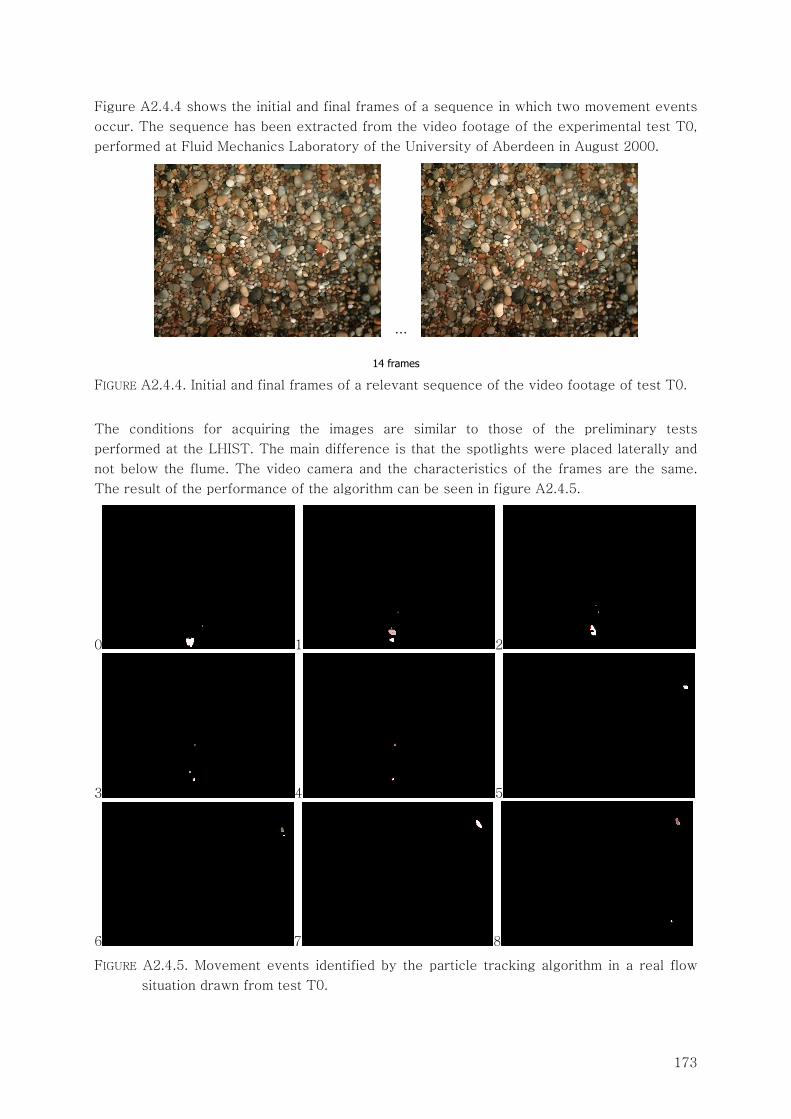
173

Figure A2.4.4 shows the initial and final frames of a sequence in which two movement events

occur. The sequence has been extracted from the video footage of the experimental test T0,

performed at Fluid Mechanics Laboratory of the University of Aberdeen in August 2000.

…

14 frames

FIGURE A2.4.4. Initial and final frames of a relevant sequence of the video footage of test T0.

The conditions for acquiring the images are similar to those of the preliminary tests

performed at the LHIST. The main difference is that the spotlights were placed laterally and

not below the flume. The video camera and the characteristics of the frames are the same.

The result of the performance of the algorithm can be seen in figure A2.4.5.

0 1 2

3 4 5

6 7 8

FIGURE A2.4.5. Movement events identified by the particle tracking algorithm in a real flow

situation drawn from test T0.

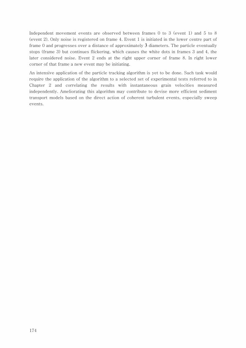
174

Independent movement events are observed between frames 0 to 3 (event 1) and 5 to 8

(event 2). Only noise is registered on frame 4. Event 1 is initiated in the lower centre part of

frame 0 and progresses over a distance of approximately 3 diameters. The particle eventually

stops (frame 3) but continues flickering, which causes the white dots in frames 3 and 4, the

later considered noise. Event 2 ends at the right upper corner of frame 8. In right lower

corner of that frame a new event may be initiating.

An intensive application of the particle tracking algorithm is yet to be done. Such task would

require the application of the algorithm to a selected set of experimental tests referred to in

Chapter 2 and correlating the results with instantaneous grain velocities measured

independently. Ameliorating this algorithm may contribute to devise more efficient sediment

transport models based on the direct action of coherent turbulent events, especially sweep

events.