(Chapter 2) SOLUTIONS TO TEXT PROBLEMS: Quick Quizzes 1. Economics is like a science because economists devise theories, collect data, and analyze

the data in an attempt to verify or refute their theories. In other words, economics is based on the scientific method.

Figure 1 shows the production possibilities frontier for a society that produces food and

clothing. Point A is an efficient point (on the frontier), point B is an inefficient point (inside the frontier), and point C is an infeasible point (outside the frontier).

Figure 1 The effects of a drought are shown in Figure 2. The drought reduces the amount of food

that can be produced, shifting the production possibilities frontier inward.

Figure 2

Microeconomics is the study of how households and firms make decisions and how they

interact in markets. Macroeconomics is the study of economy-wide phenomena, including inflation, unemployment, and economic growth.

2. An example of a positive statement is “higher taxes discourage work effort” (many other

answers are possible). That’s a positive statement because it describes the effects of higher taxes, describing the world as it is. An example of a normative statement is “the government should reduce tax rates.” That is a normative statement because it’s a claim about how the world should be.

Parts of the government that regularly rely on advice from economists are Finance

Canada in designing tax policy, Industry Canada in designing and enforcing Canada’s antimonopoly laws, and International Trade Canada in helping to negotiate trade agreements with other countries.

3. Economic advisers to the prime minister might disagree about a question of policy

because of differing scientific judgments or differences in values. Questions for Review 1. Economics is like a science because economists use the scientific method. They devise

theories, collect data, and then analyze these data in an attempt to verify or refute their theories about how the world works. Economists use theory and observation like other scientists, but they are limited in their ability to run controlled experiments. Instead, they must rely on natural experiments.

2. Economists make assumptions to simplify problems without substantially affecting the

answer. Assumptions can make the world easier to understand. 3. An economic model cannot describe reality exactly because it would be too complicated

to understand. A model is a simplification that allows the economist to see what is truly important.

4. Figure 3 shows a production possibilities frontier between milk and cookies (PPF1). If a disease kills half of the economy's cow population, less milk production is possible, so the PPF shifts inward (PPF2). Note that if the economy produces all cookies, so it doesn't need any cows, then production is unaffected. But if the economy produces any milk at all, then there will be less production possible after the disease hits.

Figure 3

5. The idea of efficiency is that an outcome is efficient if the economy is getting all it can from the scarce resources it has available. In terms of the production possibilities frontier, an efficient point is a point on the frontier, such as point A in Figure 4. A point inside the frontier, such as point B, is inefficient since more of one good could be produced without reducing the production of another good.

Figure 4 6. The two subfields in economics are microeconomics and macroeconomics.

Microeconomics is the study of how households and firms make decisions and how they interact in specific markets. Macroeconomics is the study of economy-wide phenomena.

7. Positive statements are descriptive and make a claim about how the world is, while normative statements are prescriptive and make a claim about how the world ought to be. Here is an example. Positive: A rapid growth rate of money is the cause of inflation. Normative: The government should keep the growth rate of money low.

8. The Bank of Canada sets Canada’s monetary policy. It employs more than 200

economists to analyze financial markets and macroeconomic developments. 9. Economists sometimes offer conflicting advice to policymakers for two reasons: (1) economists may disagree about the validity of alternative positive theories about

how the world works; and (2) economists may have different values and, therefore, different normative views about what public policy should try to accomplish.

Problems and Applications 1. Many answers are possible. 2. a. Steel is a fairly uniform commodity, though some firms produce steel of inferior

quality. b. Novels are each unique, so they are quite distinguishable.

c. Wheat produced by one farmer is completely indistinguishable from wheat

produced by another.

d. Fast food is more distinguishable than steel or wheat, but certainly not as much as novels.

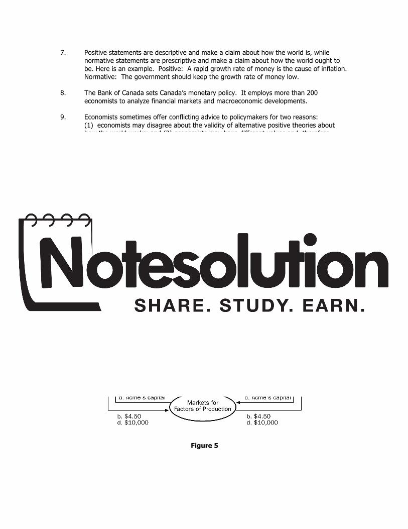
3. See Figure 5, where the four transactions are shown.

Figure 5

4. a. Figure 6 shows a production possibilities frontier between guns and butter. It is bowed out because when most of the economy’s resources are being used to produce butter, the frontier is steep and when most of the economy’s resources are being used to produce guns, the frontier is very flat. When the economy is producing a lot of guns, workers and machines best suited to making butter are being used to make guns, so each unit of guns given up yields a large increase in the production of butter. Thus, the production possibilities frontier is flat. When the economy is producing a lot of butter, workers and machines best suited to making guns are being used to make butter, so each unit of guns given up yields a small increase in the production of butter. Thus, the production possibilities frontier is steep.

b. Point A is impossible for the economy to achieve; it is outside the production

possibilities frontier. Point B is feasible but inefficient because it’s inside the production possibilities frontier.

Figure 6

c. The Hawks might choose a point like H, with many guns and not much butter. The Doves might choose a point like D, with a lot of butter and few guns.

d. If both Hawks and Doves reduced their desired quantity of guns by the same

amount, the Hawks would get a bigger peace dividend because the production possibilities frontier is much steeper at point H than at point D. As a result, the reduction of a given number of guns, starting at point H, leads to a much larger increase in the quantity of butter produced than when starting at point D.

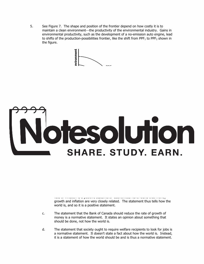
5. See Figure 7. The shape and position of the frontier depend on how costly it is to maintain a clean environment⎯the productivity of the environmental industry. Gains in environmental productivity, such as the development of a no-emission auto engine, lead to shifts of the production-possibilities frontier, like the shift from PPF1 to PPF2 shown in the figure.

Figure 7

6. a. A family's decision about how much income to save is microeconomics.

b. The effect of government regulations on auto emissions is microeconomics.

c. The impact of higher saving on economic growth is macroeconomics.

d. A firm's decision about how many workers to hire is microeconomics.

e. The relationship between the inflation rate and changes in the quantity of money is macroeconomics.

7. a. The statement that society faces a short-run tradeoff between inflation and

unemployment is a positive statement. It deals with how the economy is, not how it should be. Since economists have examined data and found that there is a short-run negative relationship between inflation and unemployment, the statement is a fact, thus it is a positive statement.

b. The statement that a reduction in the rate of growth of money will reduce the

rate of inflation is a positive statement. Economists have found that money growth and inflation are very closely related. The statement thus tells how the world is, and so it is a positive statement.

c. The statement that the Bank of Canada should reduce the rate of growth of

money is a normative statement. It states an opinion about something that should be done, not how the world is.

d. The statement that society ought to require welfare recipients to look for jobs is

a normative statement. It doesn't state a fact about how the world is. Instead, it is a statement of how the world should be and is thus a normative statement.

e. The statement that lower tax rates encourage more work and more saving is a

positive statement. Economists have studied the relationship between tax rates and work, as well as the relationship between tax rates and saving. They have found a negative relationship in both cases. The statement reflects how the world is, and is thus a positive statement.

8. Two of the statements in Table 2 are clearly normative. They are: "5. If the federal

budget is to be balanced, it should be done over the business cycle rather than yearly" and "9. The government should restructure the welfare system along the lines of a 'negative income tax.'" Both are suggestions of changes that should be made, rather than statements of fact, so they are clearly normative statements.

The other statements in the table are positive. All the statements concern how the world is, not how the world should be. Note that in all cases, even though they are statements of fact, fewer than 100 percent of economists agree with them. You could say that positive statements are statements of fact about how the world is, but not everyone agrees about what the facts are.

9. As the prime minister, you'd be interested in both the positive and normative views of

economists, but you'd probably be most interested in their positive views. Economists are on your staff to provide their expertise about how the economy works. They know many facts about the economy and the interaction of different sectors. So you would be most likely to call on them about questions of fact⎯positive analysis. Since you are the prime minister, you are the one who has to make the normative statements as to what should be done, with an eye to the political consequences. The normative statements made by economists represent their own views, not necessarily your views or the electorate’s views.

10. There are many possible answers. 11. As of this writing, the governor of the Bank of Canada is Mark J. Carney and the current

minister of Finance Canada is Jim Flaherty. Lawrence Cannon is the minister of Foreign Affairs Canada and Peter Van Loan is the minister of International Trade Canada. Carney is the only economist. Having a background in economic theory would be of significant benefit in understanding the issues and policy recommendations from each ministry to solve specific economic problems.

12. As time goes on, you might expect economists to disagree less about public policy

because they will have opportunities to observe different policies that are put into place. As new policies are tried, their results will become known, and they can be evaluated better. It's likely that the disagreement about them will be reduced after they've been tried in practice. For example, many economists thought that wage and price controls would be a good idea for keeping inflation under control, while others thought it was a bad idea. But when the controls were tried in the early 1970s, the results were disastrous. The controls interfered with the invisible hand of the marketplace and shortages developed in many markets. As a result, most economists are now convinced that wage and price controls are a bad idea for controlling inflation.

But it is unlikely that the differences between economists will ever be completely eliminated. Economists differ on too many aspects of how the world works. Plus, even as some policies get tried out and are either accepted or rejected, creative economists keep coming up with new ideas.

(Chapter 4) SOLUTIONS TO TEXT PROBLEMS: Quick Quizzes 1. A market is a group of buyers (who determine demand) and a group of sellers (who

determine supply) of a particular good or service. A competitive market is one in which there are many buyers and many sellers of an identical product so that each has a negligible impact on the market price.

2. Here’s an example of a demand schedule for pizza:

Price of Pizza Slice Number of Pizza Slices Demanded $ 0.00 10

0.25 9 0.50 8 0.75 7 1.00 6 1.25 5 1.50 4 1.75 3 2.00 2 2.25 1 2.50 0

The demand curve is graphed in Figure 1.

Figure 1

Examples of things that would shift the demand curve include changes in income, prices of related goods like soda or hot dogs, tastes, expectations about future income or prices, and the number of buyers.

A change in the price of pizza would not shift this demand curve; it would only lead us to

move from one point to another along the same demand curve. 3. Here is an example of a supply schedule for pizza:

Price of Pizza Slice Number of Pizza Slices Supplied $ 0.00 0

0.25 100 0.50 200 0.75 300 1.00 400 1.25 500 1.50 600 1.75 700 2.00 800 2.25 900 2.50 1000

The supply curve is graphed in Figure 2.

Figure 2

Examples of things that would shift the supply curve include changes in prices of inputs like tomato sauce and cheese, changes in technology like more efficient pizza ovens or automatic dough makers, changes in expectations about the future price of pizza, or a change in the number of sellers.

A change in the price of pizza would not shift this supply curve; it would only move from

one point to another along the same supply curve. 4. If the price of tomatoes rises, the supply curve for pizza shifts to the left because of the

increased price of an input into pizza production, but there is no effect on demand. The

shift to the left of the supply curve causes the equilibrium price to rise and the equilibrium quantity to decline, as Figure 3 shows.

If the price of hamburgers falls, the demand curve for pizza shifts to the left because the

lower price of hamburgers will lead consumers to buy more hamburgers and less pizza, but there is no effect on supply. The shift to the left of the demand curve causes the equilibrium price to fall and the equilibrium quantity to decline, as Figure 4 shows.

Figure 3

Figure 4 Questions for Review 1. A competitive market is a market in which there are many buyers and many sellers of an

identical product so that each has a negligible impact on the market price. Other types of markets include monopoly, in which there is only one seller, oligopoly, in which there are a few sellers that do not always compete aggressively, and monopolistically competitive markets, in which there are many sellers, each offering a slightly different product.

2. The quantity of a good that buyers demand is determined by the price of the good,

income, the prices of related goods, tastes, expectations, and the number of buyers. 3. The demand schedule is a table that shows the relationship between the price of a good

and the quantity demanded. The demand curve is the downward-sloping line relating price and quantity demanded. The demand schedule and demand curve are related because the demand curve is simply a graph showing the points in the demand schedule.

The demand curve slopes downward because of the law of demand—other things equal,

when the price of a good rises, the quantity demanded of the good falls. People buy less of a good when its price rises, both because they cannot afford to buy as much and because they switch to purchasing other goods.

4. A change in consumers' tastes leads to a shift of the demand curve. A change in price

leads to a movement along the demand curve. 5. Since Popeye buys more spinach when his income falls, spinach is an inferior good for

him. Since he buys more spinach, but the price of spinach is unchanged, his demand curve for spinach shifts out as a result of the decrease in his income.

6. The quantity of a good that sellers supply is determined by the price of the good, input

prices, technology, expectations, and the number of sellers. 7. A supply schedule is a table showing the relationship between the price of a good and

the quantity a producer is willing and able to supply. The supply curve is the upward-sloping line relating price and quantity supplied. The supply schedule and the supply curve are related because the supply curve is simply a graph showing the points in the supply schedule.

The supply curve slopes upward because when the price is high, suppliers' profits

increase, so they supply more output to the market. The result is the law of supply—other things equal, when the price of a good rises, the quantity supplied of the good also rises.

8. A change in producers' technology leads to a shift in the supply curve. A change in price

leads to a movement along the supply curve. 9. The equilibrium of a market is the point at which the quantity demanded is equal to

quantity supplied. If the price is above the equilibrium price, sellers want to sell more than buyers want to buy, so there is a surplus. Sellers try to increase their sales by cutting prices. That continues until they reach the equilibrium price. If the price is below the equilibrium price, buyers want to buy more than sellers want to sell, so there is a shortage. Sellers can raise their price without losing customers. That continues until they reach the equilibrium price.

10. When the price of beer rises, the demand for pizza declines, because beer and pizza are

complements and people want to buy less beer. When we say the demand for pizza

declines, we mean that the demand curve for pizza shifts to the left as in Figure 5. The supply curve for pizza is not affected. With a shift to the left in the demand curve, the equilibrium price and quantity both decline, as the figure shows. Thus the quantity of pizza supplied and demanded both fall. In sum, supply is unchanged, demand is decreased, quantity supplied declines, quantity demanded declines, and the price falls.

Figure 5 11. Prices play a vital role in market economies because they bring markets into equilibrium.

If the price is different from its equilibrium level, quantity supplied and quantity demanded are not equal. The resulting surplus or shortage leads suppliers to adjust the price until equilibrium is restored. Prices serve as signals that guide economic decisions and allocate scarce resources.

Problems and Applications 1. a. Cold weather damages the orange crop, reducing the supply of oranges. This

can be seen in Figure 6 as a shift to the left in the supply curve for oranges. The new equilibrium price is higher than the old equilibrium price.

Figure 6

b. People often travel to the Caribbean from Quebec to escape cold weather, so demand for Caribbean hotel rooms is high in the winter. In the summer, fewer people travel to the Caribbean, since northern climes are more pleasant. The result, as shown in Figure 7, is a shift to the left in the demand curve. The equilibrium price of Caribbean hotel rooms is thus lower in the summer than in the winter, as the figure shows.

Figure 7

c. When a war breaks out in the Middle East, many markets are affected. Since much oil production takes place there, the war disrupts oil supplies, shifting the supply curve for gasoline to the left, as shown in Figure 8. The result is a rise in the equilibrium price of gasoline. With a higher price for gasoline, the cost of operating a gas-guzzling automobile, like a SUV, will increase. As a result, the demand for used SUVs will decline, as people in the market for cars will not find SUVs as attractive. In addition, some people who already own SUVs will try to sell them. The result is that the demand curve for used SUVs shifts to the left, while the supply curve shifts to the right, as shown in Figure 9. The result is a decline in the equilibrium price of used SUVs.

Figure 8 Figure 9

2. The statement that "an increase in the demand for notebooks raises the quantity of notebooks demanded, but not the quantity supplied," in general, is false. As Figure 10 shows, the increase in demand for notebooks results in an increased quantity supplied. The only way the statement would be true is if the supply curve was a vertical line, as shown in Figure 11.

Figure 10

Figure 11

3. a. If people decide to have more children (a change in tastes), they will want larger vehicles for hauling their kids around, so the demand for minivans will increase. Supply won't be affected. The result is a rise in both price and quantity, as Figure 12 shows.

Figure 12 b. If a strike by steelworkers raises steel prices, the cost of producing a minivan

rises (a rise in input prices), so the supply of minivans decreases. Demand won't be affected. The result is a rise in the price of minivans and a decline in the quantity, as Figure 13 shows.

Figure 13

c. The development of new automated machinery for the production of minivans is an improvement in technology. The reduction in firms' costs results in an increase in supply. Demand isn't affected. The result is a decline in the price of minivans and an increase in the quantity, as Figure 14 shows.

Figure 14 d. The rise in the price of sport utility vehicles affects minivan demand because

sport utility vehicles are substitutes for minivans (that is, there is a rise in the price of a related good). The result is an increase in demand for minivans. Supply is not affected. In equilibrium, the price and quantity of minivans both rise, as Figure 12 shows.

e. The reduction in peoples' wealth caused by a stock-market crash reduces their

income, leading to a reduction in the demand for minivans, since minivans are likely a normal good. Supply isn’t affected. As a result, both price and quantity decline, as Figure 15 shows.

Figure 15

4. Technological advances that reduce the cost of producing computer chips represent a

decline in an input price for producing a computer. The result is a shift to the right in the supply of computers, as shown in Figure 16. The equilibrium price falls and the equilibrium quantity rises, as the figure shows.

Figure 16 Since computer software is a complement to computers, the lower equilibrium price of computers increases the demand for software. As Figure 17 shows, the result is a rise in both the equilibrium price and quantity of software.

Figure 17

Since typewriters are substitutes for computers, the lower equilibrium price of computers reduces the demand for typewriters. As Figure 18 shows, the result is a decline in both the equilibrium price and quantity of typewriters.

Figure 18

5. a. When a hurricane in South Carolina damages the cotton crop, it raises input prices for producing sweatshirts. As a result, the supply of sweatshirts shifts to the left, as shown in Figure 19. The new equilibrium has a higher price and lower quantity of sweatshirts.

Figure 19

b. A decline in the price of leather jackets leads more people to buy leather jackets, reducing the demand for sweatshirts. The result, shown in Figure 20, is a decline in both the equilibrium price and quantity of sweatshirts.

Figure 20

c. The effects of colleges requiring students to engage in morning calisthenics in appropriate attire raises the demand for sweatshirts, as shown in Figure 21. The result is an increase in both the equilibrium price and quantity of sweatshirts.

Figure 21

d. The invention of new knitting machines increases the supply of sweatshirts. As Figure 22 shows, the result is a reduction in the equilibrium price and an increase in the equilibrium quantity of sweatshirts.

Figure 22

6. A temporarily high birth rate in the year 2005 leads to opposite effects on the price of babysitting services in the years 2010 and 2020. In the year 2010, there are more 5-year olds who need sitters, so the demand for babysitting services rises, as shown in Figure 23. The result is a higher price for babysitting services in 2010. However, in the year 2020, the increased number of 15-year olds shifts the supply of babysitting services to the right, as shown in Figure 24. The result is a decline in the price of babysitting services.

Figure 23 Figure 24

7. Since ketchup is a complement for hot dogs, when the price of hot dogs rises, the quantity demanded of hot dogs falls, thus reducing the demand for ketchup, causing both price and quantity of ketchup to fall. Since the quantity of ketchup falls, the demand for tomatoes by ketchup producers falls, so both price and quantity of tomatoes fall. When the price of tomatoes falls, producers of tomato juice face lower input prices, so the supply curve for tomato juice shifts out, causing the price of tomato juice to fall and the quantity of tomato juice to rise. The fall in the price of tomato juice causes people to substitute tomato juice for orange juice, so the demand for orange juice declines, causing the price and quantity of orange juice to fall. Now you can see clearly why a rise in the price of hot dogs leads to a fall in price of orange juice!

Figure 25 8. It is true that the change in preferences reduces the demand for bread and that the

equilibrium price becomes lower. In the language of our demand and supply model, this change translates in a shift of the demand curve to the left. The flaw is that the new price-quantity point is located on the new demand curve, thus lower price does not reduce the quantity demanded even more. The author of the statement confuses demand with quantity demanded.

9. Quantity supplied equals quantity demanded at a price of $6 and quantity of 81 pizzas

(Figure 26). If price were greater than $6, quantity supplied would exceed quantity demanded, so suppliers would reduce their price to gain sales. If price were less than $6, quantity demanded would exceed quantity supplied, so suppliers could raise their price without losing sales. In both cases, the price would continue to adjust until it reached $6, the only price at which there is neither a surplus nor a shortage.

Figure 26 10. a. If the price of flour falls, since flour is an ingredient in bagels, the supply curve

for bagels would shift to the right. The result, shown in Figure 27, would be a fall in the price of bagels and a rise in the equilibrium quantity of bagels.

Figure 27 Since cream cheese is a complement to bagels, the fall in the equilibrium price of bagels increases the demand for cream cheese, as shown in Figure 28. The result is a rise in both the equilibrium price and quantity of cream cheese. So, a fall in the price of flour indeed raises both the equilibrium price of cream cheese and the equilibrium quantity of bagels.

Figure 28

What happens if the price of milk falls? Since milk is an ingredient in cream cheese, the fall in the price of milk leads to an increase in the supply of cream cheese. This leads to a decrease in the price of cream cheese (Figure 29), rather than a rise in the price of cream cheese. So a fall in the price of milk could not have been responsible for the pattern observed.

Figure 29

b. In part (a), we found that a fall in the price of flour led to a rise in the price of cream cheese and a rise in the equilibrium quantity of bagels. If the price of flour rose, the opposite would be true; it would lead to a fall in the price of cream cheese and a fall in the equilibrium quantity of bagels. Since the question says the equilibrium price of cream cheese has risen, it could not have been caused by a rise in the price of flour.

What happens if the price of milk rises? From part (a), we found that a fall in the price of milk caused a decline in the price of cream cheese, so a rise in the price of milk would cause a rise in the price of cream cheese. Since bagels and cream cheese are complements, the rise in the price of cream cheese would reduce the demand for bagels, as Figure 30 shows. The result is a decline in the equilibrium quantity of bagels. So a rise in the price of milk does cause both a rise in the price of cream cheese and a decline in the equilibrium quantity of bagels.

Figure 30

11. a. As Figure 31 shows, the supply curve is vertical. The constant quantity supplied makes sense because the hockey arena has a fixed number of seats no matter what the price.

Figure 31

b. Quantity supplied equals quantity demanded at a price of $8. The equilibrium

quantity is 8,000 tickets.

c. Price Quantity Demanded Quantity Supplied

$ 4 14,000 8,000 8 11,000 8,000

12 8,000 8,000 16 5,000 8,000 20 2,000 8,000

The new equilibrium price will be $12, which equates quantity demanded to quantity supplied. The equilibrium quantity is 8,000 tickets.

12. a. DVDs and TV screens are complements, because you need a screen to watch a

DVD. DVDs and movie tickets are substitutes, and TV screens and movie tickets are substitutes as well.

b. Lower costs of manufacturing TV screens shift the supply curve to the right, which decreases the equilibrium price and increases the quantity demanded and supplied. (See Figure 32.)

Quantity of Hockey Tickets

S

Price of Hockey Tickets

D

$8

8,000

Figure 32

c. The decrease in the price of TV screens increases the demand for DVDs and

decreases the demand for movie tickets, as Figure 33 shows. The price and quantity demanded of DVDs will increase. The price and quantity demanded of movie tickets will decrease.

Figure 33

Quantity of TV Screens

D

S1 S2

Price of TV Screens

Quantity of DVDs

D1

S1

Price of DVDs

D2

Quantity of Movie Tickets

D2

S1

Price of Movie Tickets

D1

13. a. Equilibrium occurs where quantity demanded is equal to quantity supplied. Thus:

Qd = Qs

1,600 – 300P = 1,400 + 700P 200 = 1,000P P = $0.20

Qd = 1,600 – 300(0.20) = 1,600 – 60 = 1,540

Qs = 1,400 + 700(0.20) = 1,400 + 140 = 1,540.

The equilibrium price of a chocolate bar is $0.20 and the equilibrium quantity is 1,540 bars.

b. Given the change in demand, equilibrium occurs where quantity demanded is

equal to quantity supplied. Thus: Qd = Qs

1,800 – 300P = 1,400 + 700P 400 = 1,000P P = $0.40

Qd = 1,800 – 300(0.40) = 1,800 – 120 = 1,680

Qs = 1,400 + 700(0.40) = 1,400 + 280 = 1,680.

The equilibrium price of a chocolate bar is $0.40 and the equilibrium quantity is 1,680 bars.

c. Given the change in supply, equilibrium occurs where quantity demanded is

equal to quantity supplied. Thus: Qd = Qs

1,600 – 300P = 1,500 + 700P 100 = 1,000P P = $0.10

Qd = 1,600 – 300(0.10) = 1,600 – 30 = 1,570

Qs = 1,500 + 700(0.10) = 1,500 + 70 = 1,570.

The equilibrium price of a chocolate bar is $0.10 and the equilibrium quantity is 1,570 bars.

14. a. Reduced police efforts would shift the supply curve to the right, while cutbacks in

education would shift the demand curve to the right. Both imply higher quantity demanded.

b. As Figure 34 shows, reduced police efforts will reduce the price of drugs, while

cutbacks in education will increase it.

Figure 34 15. The first event increases the demand for oranges, which increases both the equilibrium

price and quantity. In Figure 35, this first change corresponds to a move from point A to B. The second event increases the supply of oranges, which decreases the equilibrium price and increases the equilibrium quantity even further (a move from B to C in Figure 35). Thus, the cumulative effect on price is ambiguous (we cannot tell whether the increase in price is larger than the decrease). The effect on quantity is, however, unambiguous: the quantity traded in the market is higher.

Figure 35

Quantity of drugs

D1

S1

Price of Drugs

S2

Quantity of Drugs

D1

S

Price of Drugs

D2

Cutbacks in Education Reduced Police Efforts

Quantity of Oranges

D2

S1

Price of Oranges

S2

D1

A

B

C

(Chapter 21) SOLUTIONS TO TEXT PROBLEMS: Quick Quizzes

Figure 1

1. A person with an income of $1,000 could purchase $1,000/$5 = 200 litres of Pepsi if she spent all of her income on Pepsi or she could purchase $1,000/$10 = 100 pizzas if she spent all of her income on pizza. Thus the point representing 200 litres of Pepsi and no pizzas is the vertical intercept and the point representing 100 pizzas and no Pepsi is the horizontal intercept of the budget constraint, as shown in Figure 1. The slope of the budget constraint is the rise over the run, or -200/100 = -2.

2. Figure 2 shows indifference curves between Pepsi and pizza. The four properties of

these indifference curves are: (1) higher indifference curves are preferred to lower ones because consumers prefer more of a good to less of it; (2) indifference curves are downward sloping because if the quantity of one good is reduced, the quantity of the other good must increase in order for the consumer to be equally happy; (3) indifference curves do not cross because if they did, the assumption that more is preferred to less would be violated; and (4) indifference curves are bowed inward because people are more willing to trade away goods that they have in abundance and less willing to trade away goods of which they have little.

Figure 2

3. Figure 3 shows the budget constraint (BC1) and two indifference curves. The consumer is initially at point A, where the budget constraint is tangent to an indifference curve. The increase in the price of pizza shifts the budget constraint to BC2, and the consumer moves to point C where the new budget constraint is tangent to a lower indifference curve. To break this move down into income and substitution effects requires drawing the dashed budget line shown, which is parallel to the new budget constraint and tangent to the original indifference curve at point B. The movement from A to B represents the substitution effect, while the movement from B to C represents the income effect.

Figure 3

4. An increase in the wage can potentially decrease the amount that a person wants to work because a higher wage has an income effect that increases both leisure and consumption and a substitution effect that increases consumption and decreases leisure. Since less leisure means more work, a person will work more only if the substitution effect outweighs the income effect.

Questions for Review

Figure 4

1. Figure 4 shows the consumer's budget constraint. The intercept on the horizontal axis shows how much cheese the consumer could buy if she bought only cheese; with income of $3,000 and the price of cheese $6 a kilogram, she could buy 500 kilograms of cheese. The intercept on the vertical axis shows how much wine the consumer could buy if she bought only wine; with income of $3,000 and the price of wine $3 a glass, she could buy 1,000 glasses of wine. With cheese on the horizontal axis and wine on the vertical axis, the budget constraint has a slope of -1,000/500 = -2. Note that if you would put wine on the horizontal axis and cheese on the vertical axis, the budget constraint would have a slope of -500/1,000 = -1/2.

2. Figure 5 shows a consumer's indifference curves for wine and cheese. Four properties of

these indifference curves are: (1) higher indifference curves are preferred to lower ones because more is preferred to less; (2) indifference curves are downward sloping because if the quantity of wine is reduced, the quantity of cheese must increase for the consumer to be equally happy; (3) indifference curves do not cross since a consumer prefers more to less; and (4) indifference curves are bowed inward since a consumer is more willing to trade away wine if she has a lot of it and less willing to trade away cheese if she has little of it.

Figure 5 3. In Figure 5, the marginal rate of substitution (MRS) of one point on an indifference curve

is shown. The marginal rate of substitution shows the amount of wine the consumer would be willing to give up to get one more kilogram of cheese.

4. Figure 6 shows the consumer's budget constraint and indifference curves for wine and

cheese. The consumer's optimum consumption choice is shown as w* and c*. Since the marginal rate of substitution equals the relative price of the two goods at the optimum, the marginal rate of substitution is $6/$3 = 2.

Figure 6 5. Figure 7 shows the effect of an increase in income. The rise in income shifts the budget

constraint out from BC1 to BC2. If both wine and cheese are normal goods, consumption of both increases. If cheese is an inferior good, the increase in income causes the consumption of cheese to decline, as shown in Figure 8.

Figure 7

Figure 8

Figure 9 6. A rise in the price of cheese from $6 to $10 a kilogram makes the horizontal intercept of

the budget line decline from 500 to 300, as shown in Figure 9. The consumer's budget constraint shifts from BC1 to BC2 and her optimal choice changes from point A (c1 cheese, w1 wine) to point B (c2 cheese, w2 wine). To decompose this change into income and substitution effects, we draw in budget constraint BC3, which is parallel to BC2 but tangent to the consumer's initial indifference curve at point C. The movement from point A to C represents the substitution effect. Since cheese became more expensive, the consumer substitutes wine for cheese as she moves from point A to C. The movement from point C to B represents an income effect. The rise in the price of cheese results in an effective decline in income.

7. An increase in the price of cheese could induce a consumer to buy more cheese if cheese is a Giffen good. In that case, the income effect of the rise in the price of cheese induces the consumer to buy more cheese if cheese is an inferior good. If the income effect is bigger than the substitution effect (which induces the consumer to buy less cheese), the consumer would buy more cheese.

Problems and Applications 1. a. Figure 10 shows the effect of the frost on Jennifer's budget constraint. Since the

price of coffee rises, her budget constraint swivels from BC1 to BC2.

b. If the substitution effect outweighs the income effect for croissants, Jennifer buys more croissants and less coffee, as shown in Figure 10. She moves from point A to point B.

Figure 10

c. If the income effect outweighs the substitution effect for croissants, Jennifer buys fewer croissants and less coffee, moving from point A to point B in Figure 11.

Figure 11

2. Indifference curves between Coke and Pepsi are fairly straight, since there is little to distinguish them, so they are nearly perfect substitutes. Indifference curves between skis and ski bindings are very bowed, since they are complements. A consumer will respond more to a change in the relative price of Coke and Pepsi, possibly switching completely from one to the other if the price changes.

3. a. Cheese and crackers cannot both be inferior goods, since if Mario's income rises

he must consume more of something.

b. If the price of cheese falls, the substitution effect means Mario will consume more cheese and fewer crackers. The income effect means Mario will consume more cheese (since cheese is a normal good) and fewer crackers (since crackers are an inferior good). So, both effects lead Mario to consume more cheese and fewer crackers.

Figure 12

4. a. Figure 12 shows Jim's budget constraint. The vertical intercept is 50 litres of milk, since if Jim spent all his money on milk he would buy $100/$2 = 50 litres of it. The horizontal intercept is 25 dozen cookies, since if Jim spent all his money on cookies he would buy $100/$4 = 25 dozen cookies.

b. If Jim's salary rises by 10 percent to $110 and the prices of milk and cookies rise

by 10 percent to $2.20 and $4.40, Jim's budget constraint would be unchanged. Note that $110/$2.20 = 50 and $110/$4.40 = 25, so the intercepts of the new budget constraint would be the same as the old budget constraint. Since the budget constraint is unchanged, Jim's optimal consumption is unchanged.

Figure 13

Figure 14 5. a. Budget constraint BC1 in Figure 13 shows the budget constraint if you pay no

taxes. Budget constraint BC2 shows the budget constraint with a 15 percent tax.

b. Figure 14 shows indifference curves for which a person will work more as a result of the tax because the income effect (less leisure) outweighs the substitution effect (more leisure), so there is less leisure overall. Figure 15 shows indifference curves for which a person will work fewer hours as a result of the tax because the income effect (less leisure) is smaller than the substitution effect (more leisure), so there is more leisure overall. Figure 16 shows indifference curves for which a person will work the same number of hours after the tax because the income effect (less leisure) equals the substitution effect (more leisure), so there is the same amount of leisure overall.

Figure 15

Figure 16 6. Figure 17 shows Sarah's budget constraints and indifference curves if she earns $6 (BC1),

$8 (BC2), and $10 (BC3) per hour. At a wage of $6 per hour, she works 100 - L6 hours; at a wage of $8 per hour, she works 100 - L8 hours; and at a wage of $10 per hour, she works 100 - L10 hours. Since the labour supply curve is upward sloping when the wage is between $6 and $8 per hour, L6 > L8; since the labour supply curve is backward sloping when the wage is between $8 and $10 per hour, L10 > L8.

Figure 17

Figure 18 7. Figure 18 shows the indifference curve between leisure and consumption that determines

how much a person works. An increase in the wage leads to both an income effect and a substitution effect. The higher wage makes the budget constraint steeper, so the substitution effect increases consumption and reduces leisure. But the higher wage has an income effect that increases both consumption and leisure if both are normal goods. The only way that consumption could decrease when the wage increased would be if consumption is an inferior good and if the negative income effect outweighs the positive substitution effect. This could happen for a person who really placed an exceptionally high value on leisure.

Figure 19 8 a. Figure 19 shows the situation in which your salary increases from $30,000 to

$40,000. With numbers shown in thousands of dollars in the figure, your initial budget constraint, BC1, has a horizontal intercept of 30, since you could spend all your income when young. The vertical intercept is 31.5, since if you spent nothing when young and saved all your income, earning 5 percent interest, you would have $31,500 to spend when old. If your salary increases to $40,000, your budget constraint shifts out in a parallel fashion, with intercepts of 40 and 42, respectively. This is an income effect only, so if consumption when young and old are both normal goods, you will spend more in both periods.

b. If the interest rate on your bank account rises to 8 percent, your budget

constraint rotates. If you spend all your income when young, you will spend just $30,000, as before. But if you save all your income, your old-age consumption increases to $30,000 x 1.08 = $32,400, compared to $31,500 before. As Figure 20 indicates, the steeper budget line leads you to substitute future consumption for current consumption. But the income effect of the higher return on your saving leads you to want to increase both future and current consumption if both are normal goods. The result is that your consumption when old certainly rises and your consumption when young could increase or decrease, depending on whether the income or substitution effect dominates.

Figure 20

9. The decline in the interest rate on savings has both income and substitution effects, since it causes the budget constraint to rotate. Since consumption when old effectively becomes more expensive relative to consumption when young, there is a substitution effect that increases consumption when young and decreases consumption when old. The lower interest rate also leads to a negative income effect, causing both consumption when young and consumption when old to decline if both are normal goods. Combining both effects, consumption when old definitely declines and consumption when young might rise or fall, depending on whether the income or substitution effect is stronger.

10. a. Figure 21 shows the effects of the welfare system. Without the system, the

budget constraint would begin on the horizontal axis at point Lmax when the family earns no labour income and would have a slope equal to the wage rate. The system provides income of a certain amount if the family earns no labour income, shown as the point A on the figure. Then, if income is earned, the welfare payment is reduced, so the slope of the budget line is less than the slope of the budget line without welfare. At the point where the two budget lines meet, the welfare system provides no further support.

b. The figure shows how indifference curves could be shaped, indicating a reduction

in the number of hours worked by the family because of the welfare system. Since the welfare budget constraint is flatter, there is a substitution effect away from consumption and towards leisure. Since the welfare budget constraint is farther from the origin, there is an income effect that increases both consumption and leisure, if both are normal goods. The overall effect is that the change in consumption is ambiguous and the family will want to have more leisure; hence, it will reduce its labour supply.

c. There is no doubt that the family's well-being is increased, since the welfare

system gives them consumption and leisure opportunities that were not available before and they end up on a higher indifference curve.

Figure 21

Figure 22 11. If consumers do not buy less of a good when their incomes rise, the good in question

must be a normal good. For a normal good, the income and substitution effects both imply that the consumer will buy less if the price rises.

12. A College Student’s decision Making under Budget Constraint

a. Let H stand for the number of meals at the dining hall and S the number of meals at Cup O’Soup. The budget constraint must equate expenditure on all meals to the budget of $60, that is 6×H+1.5×S=60. If the consumer chooses to eat only at the dining hall, she can afford H=60/6=10 meals. If she chooses only Cup O’Soup meals. She can afford a total of S=60/1.5=40 meals. These are the intercepts of the budget line in our graph. Figure 23 shows the budget line. The tradeoff is 10/40=1.5/6=1/4 meals at dining hall for one meal at Cup O’Soup. If the consumer spends equal amounts on H and S, the equation 1.5×S=6×H must

hold, which gives S=(6/1.5)H=4H. If we replace this value of S in the budget equation, we get 6H=1.5×4H=60. Solving this equation gives H=60/(6+1.5×4)=60/12=5 meals at dining hall. The corresponding number of meals at Cup O’Soup is S=4H=4×5=20. We can check now that 5 meals at dining hall and 20 meals at Cup O’Soup are together $60, as follows: 6×5+1.5×20=30+30=$60.

Figure 23

b. When the price of Cup O’Sup increases to $2, the budget line rotates toward less

Cup O’Soup meals, as shown in Figure 23. Now H and S must satisfy, besides the budget equation, the new spending pattern, described by the equation 0.3×6H=0.7×2S. This gives S=1.29H. Replace this in the new budget equation: 6H+2×1.29H=60. The solution is the optimal number of dining hall meals, H=60/(6+2×1.29)=7. The optimal number of meals at Cup O’Soup is now S=1.29×7=9. The new consumption point is point B in Figure 23.

c. When the price of Cups O’Soup increased, the quantity consumed decreased; this shows that the substitution effect is stronger than the income effect.

d. The demand curve for Cup O’Soup is downward sloping, as Figure 24 shows. Cup O’Soup is a normal good.

H, number

of meals at dining

hall

S, number of meals at Cup O’Soup

Budget line; the slope shows the tradeoff ¼ dining hall meals for one Cup O’Soup meal

10

40

5

20

A B 7

30

9

Figure 24

13. Deciding How Many Children to Have

a. Let K be the number of children. Let K be the number of children and C life time

consumption. If the couple has no kids, the couple can consume 200,000×$10=$2 million. If they consume nothing (of course an unrealistic assumption), they can have 200.000/20,000=10 children. The couple has to give up $200.000 in consumption for each additional child. Figur 25 shows this budget line.

b. If wage increases to $12, the maximum possible number of children does not change because is limited by time, but the maximum consumption for zero children increases to 200,000×$12=$2.4 million. The new budget line becomes steeper, which shows that the opportunity cost of raising children has increased. The choice point moves toward higher consumption, from A to B. Whether the couple chooses to have more or less children depends on their preferences. If the substitution effect is stronger than the income effect, then the couple will have less children and the other way around.

c. The observation is consistent with our model and shows that people perceive children as a normal “good”.

Price of Cup

O’Soup

Quantity of Cups O’Soup

$2

$1.5

9 20

A

B

Figure 25

14. The market values apples twice as much as pears given their relative price. Jerry values

apples twice as much as pears too; thus, he does not want to change his choice. George is willing to give up an apple for a pear, but in the market he can get two pears for that apple. Thus, George is better off if he gives up some apples in exchange for pears. Elaine is in the same situation as Jerry, so she is at optimum. Kramer values pears even more than George, so Kramer should give up apples for pears. Newman’s valuation of apples is more than the market, so he should give up pears in exchange for apples.

K (number of children)

A

B

10

2 mil

2.4 mil

C (Consumption)

(Chapter 5) SOLUTIONS TO TEXT PROBLEMS: Quick Quizzes 1. The price elasticity of demand is a measure of how much the quantity demanded of a

good responds to a change in the price of that good, computed as the percentage change in quantity demanded divided by the percentage change in price.

The relationship between total revenue and the price elasticity of demand is: (1) when

demand is inelastic (a price elasticity less than 1), a price increase raises total revenue, and a price decrease reduces total revenue; (2) when demand is elastic (a price elasticity greater than 1), a price increase reduces total revenue, and a price decrease raises total revenue; and (3) when demand is unit elastic (a price elasticity equal to 1), a change in price does not affect total revenue.

2. The price elasticity of supply is a measure of how much the quantity supplied of a good

responds to a change in the price of that good, computed as the percentage change in quantity supplied divided by the percentage change in price.

The price elasticity of supply might be different in the long run than in the short run

because over short periods of time, firms cannot easily change the size of their factories to make more or less of a good. Thus, in the short run, the quantity supplied is not very responsive to the price. However, over longer periods, firms can build new factories, expand existing factories, or close old ones, or they can enter or exit a market. So, in the long run, the quantity supplied can respond substantially to the price.

3. A drought that destroys half of all farm crops could be good for farmers (at least those

unaffected by the drought) if the demand for the crops is inelastic. The shift to the left of the supply curve leads to a price increase that raises total revenue because the price elasticity is less than one.

Even though a drought could be good for farmers, they would not destroy their crops in

the absence of a drought because no one farmer would have an incentive to destroy his crops, since he takes the market price as given. Only if all farmers destroyed their crops together, for example through a government program, would this plan work to make farmers better off.

Questions for Review 1. The price elasticity of demand measures how much the quantity demanded responds to

a change in price. The income elasticity of demand measures how much the quantity demanded responds to changes in consumer income.

2. The determinants of the price elasticity of demand include how available close

substitutes are, whether the good is a necessity or a luxury, how broadly defined the market is, and the time horizon. Luxury goods have greater price elasticities than necessities, goods with close substitutes have greater elasticities, goods in more narrowly defined markets have greater elasticities, and the elasticity of demand is higher the longer the time horizon.

3. An elasticity greater than one means that demand is elastic. When the elasticity is

greater than one, the percentage change in quantity demanded exceeds the percentage change in price. When the elasticity equals zero, demand is perfectly inelastic. There is no change in quantity demanded when there is a change in price.

4. Figure 1 presents a supply-and-demand diagram, showing equilibrium price, equilibrium

quantity, and the total revenue received by producers. Total revenue equals the equilibrium price times the equilibrium quantity, which is the area of the rectangle shown in the figure.

Figure 1

5. If demand is elastic, an increase in price reduces total revenue. With elastic demand, the quantity demanded falls by a greater percentage than the percentage increase in price. As a result, total revenue declines.

6. A good with an income elasticity less than zero is called an inferior good because as

income rises, the quantity demanded declines. 7. The price elasticity of supply is calculated as the percentage change in quantity supplied

divided by the percentage change in price. It measures how much the quantity supplied responds to changes in the price.

8. The price elasticity of supply of Picasso paintings is zero, since no matter how high price rises, no more can ever be produced.

9. The price elasticity of supply is usually larger in the long run than it is in the short run.

Over short periods of time, firms cannot easily change the size of their factories to make more or less of a good, so the quantity supplied is not very responsive to price. Over longer periods, firms can build new factories or close old ones, so the quantity supplied is more responsive to price.

10. The midpoint method of calculating elasticity has the advantage that it gives the same

result whether one starts from point A to B or from B to A. 11 Since the demand for drugs is inelastic, a reduction in supply increases the price by a

higher percentage that it reduces the quantity demanded; therefore, the reduction in supply increases the revenue to sellers. Drug addicts have to pay more; those who had to steal before the interdiction will steal even more. Thus, drug-related crime may actually increase because of the interdiction.

Problems and Applications 1. a. Mystery novels have more elastic demand than required textbooks, because

mystery novels have close substitutes and are a luxury good, while required textbooks are a necessity with no close substitutes. If the price of mystery novels were to rise, readers could substitute other types of novels, or buy fewer novels altogether. But if the price of required textbooks were to rise, students would have little choice but to pay the higher price. Thus the quantity demanded of required textbooks is less responsive to price than the quantity demanded of mystery novels.

b. Beethoven recordings have more elastic demand than classical music recordings

in general. Beethoven recordings are a narrower market than classical music recordings, so it's easy to find close substitutes for them. If the price of Beethoven recordings were to rise, people could substitute other classical recordings, like Mozart. But if the price of all classical recordings were to rise, substitution would be more difficult (a transition from classical music to rap is unlikely!). Thus the quantity demanded of classical recordings is less responsive to price than the quantity demanded of Beethoven recordings.

c. Heating oil during the next five years has more elastic demand than heating oil

during the next six months. Goods have a more elastic demand over longer time horizons. If the price of heating oil were to rise temporarily, consumers couldn't switch to other sources of fuel without great expense. But if the price of heating oil were to be high for a long time, people would gradually switch to gas or electric heat. As a result, the quantity demanded of heating oil during the next six months is less responsive to price than the quantity demanded of heating oil during the next five years.

d. Root beer has more elastic demand than water. Root beer is a luxury with close

substitutes, while water is a necessity with no close substitutes. If the price of water were to rise, consumers have little choice but to pay the higher price. But if the price of root beer were to rise, consumers could easily switch to other sodas. So the quantity demanded of root beer is more responsive to price than the quantity demanded of water.

2. a. For business travelers, the price elasticity of demand when the price of tickets rises from $200 to $250 is [(2,000 - 1,900)/1,950]/[(250 - 200)/225] = 0.05/0.22 = 0.23. For vacationers, the price elasticity of demand when the price of tickets rises from $200 to $250 is [(800 - 600)/700] / [(250 - 200)/225] = 0.29/0.22 = 1.32.

b. The price elasticity of demand for vacationers is higher than the elasticity for

business travelers because vacationers can choose more easily a different mode of transportation (like driving or taking the train). Business travelers are less likely to do so since time is more important to them and their schedules are less adaptable.

3. a. If your income is $10,000, your price elasticity of demand as the price of

compact discs rises from $8 to $10 is [(40 - 32)/36]/[(10 - 8)/9] =0.22/0.22 = 1. If your income is $12,000, the elasticity is [(50 - 45)/47.5]/[(10 - 8)/9] = 0.11/0.22 = 0.5.

b. If the price is $12, your income elasticity of demand as your income increases

from $10,000 to $12,000 is [(30 - 24)/27] / [(12,000 - 10,000)/11,000] = 0.22/0.18 = 1.22. If the price is $16, your income elasticity of demand as your income increases from $10,000 to $12,000 is [(12 - 8)/10] / [(12,000 - 10,000)/11,000] = 0.40/0.18 = 2.2.

4. a. If Emily always spends one-third of her income on clothing, then her income

elasticity of demand is one, since maintaining her clothing expenditures as a constant fraction of her income means the percentage change in her quantity of clothing must equal her percentage change in income. For example, suppose the price of clothing is $30, her income is $9,000, and she purchases 100 clothing items. If her income rose 10 percent to $9,900, she'd spend a total of $3,300 on clothing, which is 110 clothing items, a 10 percent increase.

b. Emily's price elasticity of clothing demand is also one, since every percentage

point increase in the price of clothing would lead her to reduce her quantity purchased by the same percentage. Again, suppose the price of clothing is $30, her income is $9,000, and she purchases 100 clothing items. If the price of clothing rose 1 percent to $30.30, she would purchase 99 clothing items, a 1 percent reduction. [Note: This part of the problem can be confusing to students if they have an example with a larger percentage change and they use the point elasticity. Only for a small percentage change will the answer work with an elasticity of one. Alternatively, they can get the second part if they use the midpoint method for any size change.]

c. Since Emily spends a smaller proportion of her income on clothing, then for any

given price, her quantity demanded will be lower. Thus her demand curve has shifted to the left. But because she'll again spend a constant fraction of her income on clothing, her income and price elasticities of demand remain one.

5. a. The percent change in quantity demand is (2.92-2.62)/2.77 which is 2.46%. The

price elasticity of demand is 2.47/22 = 0.11.

b. Given that the price elasticity of demand is inelastic (less than one), an increase in the price of milk will increase total revenue.

c. Recall from Chapter 4 that a movement along a demand curve is called a

“change in quantity demanded”, brought about by a change in the price of the good we are considering. So, in this article, it states that a price increase leads to a fall in demand when it should have stated a fall in quantity demanded. A movement up the demand curve due to the price increase may put you into the elastic range of the demand elasticity as opposed to the inelastic demand that we calculated.

6. Tom's price elasticity of demand is zero, since he wants the same quantity regardless of the price. Jerry's price elasticity of demand is one, since he spends the same amount on gas, no matter what the price, which means his percentage change in quantity is equal to the percentage change in price.

7. The answer depends on the elasticity of demand. If the demand for visits is inelastic,

then an increase in the price of admission would increase total revenue. But if the demand is elastic, then an increase in price would cause the number of visitors to fall by so much that total revenue would decrease.

8. a. With a price elasticity of demand of 0.4, reducing the quantity demanded of

cigarettes by 20 percent requires a 50 percent increase in price, since 20/50 = 0.4. With the price of cigarettes currently $8, this would require an increase in the price to $3.33 a pack using the midpoint method (note that ($13.30 - $8)/$10.67 = 0.50).

b. The policy will have a larger effect five years from now than it does one year

from now. The elasticity is larger in the long run, since it may take some time for people to reduce their cigarette usage. The habit of smoking is hard to break in the short run.

c. Since teenagers don't have as much income as adults, they are likely to have a

higher price elasticity of demand. Also, adults are more likely to be addicted to cigarettes, making it more difficult to reduce their quantity demanded in response to a higher price.

9. a. With a price elasticity of demand of 0.2 in the short run, increasing the price from

$0.45 to $0.55 would cause the quantity demanded of heating oil to drop by 4%, since 0.04/0.2 = 0.2. In the long run, the same increase in price would cause the quantity demand to drop by 14%, since 0.14/0.2 = 0.7.

b. In the short-run, households cannot easily switch from heating oil to other

alternative fuels, so the quantity demanded drops only slightly given the price increase. In the long-run, households can search for or use other means to heat their homes so the quantity demanded for heating oil tends to drop more significantly.

10. a. As Figure 2 shows, in both markets, the increase in supply reduces the

equilibrium price and increases the equilibrium quantity. b. In the market for pharmaceutical drugs, with inelastic demand, the increase in

supply leads to a relatively large decline in the price and not much of an increase in quantity.

Figure 2 c. In the market for computers, with elastic demand, the increase in supply leads to

a relatively large increase in quantity and not much of a decline in price. d. In the market for pharmaceutical drugs, since demand is inelastic, the

percentage increase in quantity will be less than the percentage decrease in price, so total consumer spending will decline. In contrast, since demand is elastic in the market for computers, the percentage increase in quantity will be greater than the percentage decrease in price, so total consumer spending will increase.

11. a. As Figure 3 shows, in both markets the increase in demand increases both the

equilibrium price and the equilibrium quantity. b. In the market for beachfront resorts, with inelastic supply, the increase in

demand leads to a relatively large increase in the price and not much of an increase in quantity.

c. In the market for automobiles, with elastic supply, the increase in demand leads

to a relatively large increase in quantity and not much of an increase in price. d. In both markets, total consumer spending rises, since both equilibrium price and

equilibrium quantity rise.

Figure 3 12. a. Farmers whose crops weren't destroyed benefited because the destruction of

some of the crops reduced the supply, causing the equilibrium price to rise.

b. To tell whether farmers as a group were hurt or helped by the floods, you'd need to know the price elasticity of demand. It could be that the additional income earned by farmers whose crops weren't destroyed rose more because of the higher prices than farmers whose crops were destroyed, if demand is inelastic.

13. A worldwide drought could increase the total revenue of farmers if the price elasticity of

demand for grain is inelastic. The drought reduces the supply of grain, but if demand is inelastic, the reduction of supply causes a large increase in price. Total farm revenue would rise as a result. If there's only a drought in Alberta, Albertas’ production isn't a large enough proportion of the total farm product to have much impact on the price. As a result, price does not change (or changes by only a slight amount), while the output of Alberta farmers declines, thus reducing their income.

14. The decrease in quantity must have been determined by an increase in price. Since the

increase in price makes revenue to increase, the demand curve must be inelastic. 15. Billy could be right. An increase in demand would imply a rise in price when supply is

perfectly inelastic. Marian cannot be right because when demand and supply increase the effect on price is ambiguous, but the quantity must increase. Valerie could be right: a decrease in supply increases the price, and if the demand is totally inelastic the equilibrium quantity does not change. Figure 4 illustrates the three situations.

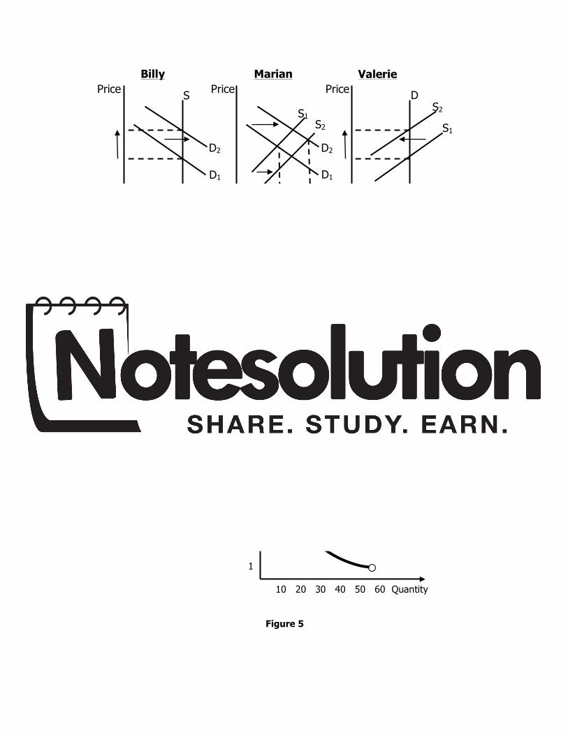
Figure 4

16 Yes. First, the negative income elasticity of good X shows that X is an inferior good:

when income increases the demand for X decreases. Second, goods X and Y are substitutes, as the positive cross price elasticity shows. This implies that a decrease in the price of Y decreases the demand for X. Thus, both events, an increase in income and a decrease in the price of Y make the demand for X shift in the same direction, namely towards lower quantities.

17 The quantity demanded at different prices is calculated in the Table 1. Figure 5 shows

the corresponding graph. The midpoint price elasticity of demand between P=1 and P=2 is equal to [(30�60)/45]/[(2�1)/1.5]=�1; The midpoint price elasticity between the prices 5 and 6 is equal to [(10�12)/11]/[(6�5)/5.5]=�1. The demand curve has constant elasticity, as opposed to a linear demand curve where the elasticity changes when the price changes.

Figure 5

S

D2

D1

Quantity

Price

S1

D2

D1

Quantity

Price D S2

S1

Quantity

Price

S2

Price

Quantity 10 20 30 40 50 60

6

5

4

3

2

1

Price Quantity= 60/Price

$1 60 2 30 3 20 4 15 5 12 6 10

Billy Valerie Marian

(Chapter 6) SOLUTIONS TO TEXT PROBLEMS: Quick Quizzes 1. A price ceiling is a legal maximum on the price at which a good can be sold. Examples of

price ceilings include rent control, price controls on gasoline in the 1970s, and price ceilings on water during a drought. A price floor is a legal minimum on the price at which a good can be sold. Examples of price floors include the minimum wage and farm-support prices. A price ceiling leads to a shortage, if the ceiling is binding, because suppliers won’t produce enough goods to meet demand unless the price is allowed to rise above the ceiling. A price floor leads to a surplus, if the floor is binding, because suppliers produce more goods than are demanded unless the price is allowed to fall below the floor.

2. With no tax, as shown in Figure 1, the demand curve is D1 and the supply curve is S. The

equilibrium price is P1 and the equilibrium quantity is Q1. If the tax is imposed on car buyers, the demand curve shifts down by the amount of the tax ($1,000) to D2. The downward shift in the demand curve leads to a decline in the equilibrium price to P2 (the amount received by sellers from buyers) and a decline in the equilibrium quantity to Q2. The price received by sellers declines by P1 – P2, shown in the figure as Δ PS. Buyers pay a total of P2 + $1,000, an increase in what they pay of P2 + $1,000 - P1, shown in the figure as Δ PB.

Figure 1

If the tax is imposed on car sellers, as shown in Figure 2, the supply curve shifts up by

the amount of the tax ($1,000) to S2. The upward shift in the supply curve leads to a rise in the equilibrium price to P2 (the amount received by sellers from buyers) and a decline in the equilibrium quantity to Q2. The price paid by buyers declines by P1 - P2, shown in the figure as ΔPB. Sellers receive P2 and pay taxes of $1,000, receiving on net P2 - $1,000, a decrease in what they receive by P1 - (P2 - $1,000), shown in the figure as ΔPS.

Figure 2 Questions for Review 1. An example of a price ceiling is the rent control system in New York City. An example of

a price floor is the minimum wage. Many other examples are possible. 2. A shortage of a good arises when there is a binding price ceiling. A surplus of a good

arises when there is a binding price floor. 3. When the price of a good is not allowed to bring supply and demand into equilibrium,

some alternative mechanism must allocate resources. If quantity supplied exceeds quantity demanded, so that there is a surplus of a good as in the case of a binding price floor, sellers may try to appeal to the personal biases of the buyers. If quantity demanded exceeds quantity supplied, so that there is a shortage of a good as in the case of a binding price ceiling, sellers can ration the good according to their personal biases, or make buyers wait in line.

4. Economists usually oppose controls on prices because prices have the crucial job of

coordinating economic activity by balancing demand and supply. When policymakers set controls on prices, they obscure the signals that guide the allocation of society’s resources. Further, price controls often hurt those they are trying to help.

5. A tax paid by buyers shifts the demand curve, while a tax paid by sellers shifts the supply

curve. However, the outcome is the same regardless of who pays the tax. 6. A tax on a good raises the price buyers pay, lowers the price sellers receive, and reduces

the quantity sold. 7. The burden of a tax is divided between buyers and sellers depending on the elasticity of

demand and supply. Elasticity represents the willingness of buyers or sellers to leave the market, which in turns depends on their alternatives. When a good is taxed, the side of the market with fewer good alternatives cannot easily leave the market and thus bears more of the burden of the tax.

Problems and Applications

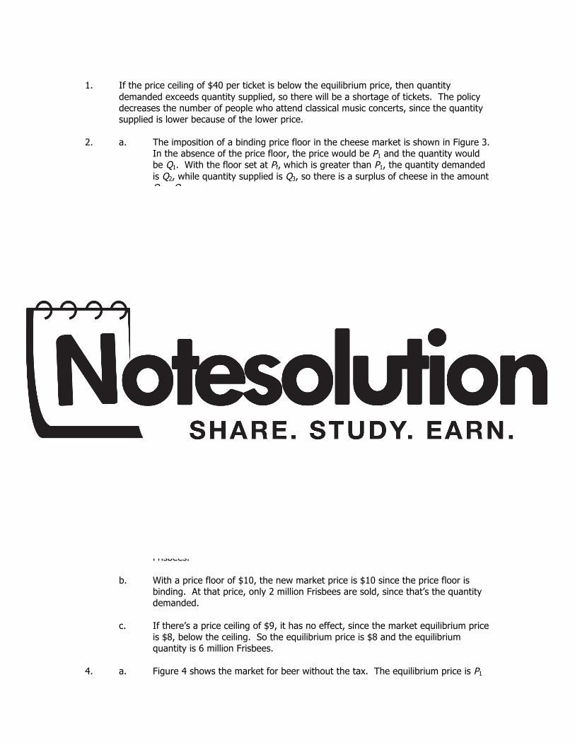
1. If the price ceiling of $40 per ticket is below the equilibrium price, then quantity

demanded exceeds quantity supplied, so there will be a shortage of tickets. The policy decreases the number of people who attend classical music concerts, since the quantity supplied is lower because of the lower price.

2. a. The imposition of a binding price floor in the cheese market is shown in Figure 3.

In the absence of the price floor, the price would be P1 and the quantity would be Q1. With the floor set at Pf, which is greater than P1, the quantity demanded is Q2, while quantity supplied is Q3, so there is a surplus of cheese in the amount Q3 – Q2.

b. The farmers’ complaint that their total revenue has declined is correct if demand

is elastic. With elastic demand, the percentage decline in quantity would exceed the percentage rise in price, so total revenue would decline.

c. If the government purchases all the surplus cheese at the price floor, producers

benefit and taxpayers lose. Producers would produce quantity Q3 of cheese, and their total revenue would increase substantially. But consumers would buy only quantity Q2 of cheese, so they are in the same position as before. Taxpayers lose because they would be financing the purchase of the surplus cheese through higher taxes.

Figure 3 3. a. The equilibrium price of Frisbees is $8 and the equilibrium quantity is 6 million

Frisbees.

b. With a price floor of $10, the new market price is $10 since the price floor is binding. At that price, only 2 million Frisbees are sold, since that’s the quantity demanded.

c. If there’s a price ceiling of $9, it has no effect, since the market equilibrium price

is $8, below the ceiling. So the equilibrium price is $8 and the equilibrium quantity is 6 million Frisbees.

4. a. Figure 4 shows the market for beer without the tax. The equilibrium price is P1

and the equilibrium quantity is Q1. The price paid by consumers is the same as the price received by producers.

Figure 4

Figure 5 b. When the tax is imposed, it drives a wedge of $2 between supply and demand,

as shown in Figure 5. The price paid by consumers is P2, while the price received by producers is P2 – $2. The quantity of beer sold declines to Q2.

5. Reducing the payroll tax paid by firms and using part of the extra revenue to reduce the

payroll tax paid by workers would not make workers better off, because the division of the burden of a tax depends on the elasticity of supply and demand and not on who must pay the tax. Since the tax wedge would be larger, it is likely that both firms and workers, who share the burden of any tax, would be worse off.

6. If the government imposes a $500 tax on luxury cars, the price paid by consumers will rise less than $500, in general. The burden of any tax is shared by both producers and consumers⎯the price paid by consumers rises and the price received by producers falls, with the difference between the two equal to the amount of the tax. The only exceptions would be if the supply curve were perfectly elastic or the demand curve were perfectly inelastic, in which case consumers would bear the full burden of the tax and the price paid by consumers would rise by exactly $500.

7. a. It doesn’t matter whether the tax is imposed on producers or consumers⎯the

effect will be the same. With no tax, as shown in Figure 6, the demand curve is D1 and the supply curve is S1. If the tax is imposed on producers, the supply curve shifts up by the amount of the tax (50 cents) to S2. Then the equilibrium quantity is Q2, the price paid by consumers is P2, and the price received (after taxes are paid) by producers is P2 – 50 cents. If the tax is instead imposed on consumers, the demand curve shifts down by the amount of the tax (50 cents) to D2. The downward shift in the demand curve (when the tax is imposed on consumers) is exactly the same magnitude as the upward shift in the supply curve when the tax is imposed on producers. So again, the equilibrium quantity is Q2, the price paid by consumers is P2 (including the tax paid to the government), and the price received by producers is P2 – 50 cents.

Figure 6

b. The more elastic is the demand curve, the more effective this tax will be in reducing the quantity of gasoline consumed. Greater elasticity of demand means that quantity falls more in response to the rise in the price of gasoline. Figure 7 illustrates this result. Demand curve D1 represents an elastic demand curve, while demand curve D2 is more inelastic. To get the same tax wedge between demand and supply requires a greater reduction in quantity with demand curve D1 than for demand curve D2.

Figure 7

c. The consumers of gasoline are hurt by the tax because they get less gasoline at a higher price.

d. Workers in the oil industry are hurt by the tax as well. With a lower quantity of

gasoline being produced, some workers may lose their jobs. With a lower price received by producers, wages of workers might decline.

8. a. Figure 8 shows the effects of the minimum wage. In the absence of the

minimum wage, the market wage would be w1 and Q1 workers would be employed. With the minimum wage (wm) imposed above w1, the market wage is wm, the number of employed workers is Q2, and the number of workers who are unemployed is Q3 - Q2. Total wage payments to workers are shown as the area of rectangle ABCD, which equals wm times Q2.

Figure 8

b. An increase in the minimum wage would decrease employment. The size of the effect on employment depends only on the elasticity of demand. The elasticity of supply doesn’t matter, because there’s a surplus of labour.

c. The increase in the minimum wage would increase unemployment. The size of

the rise in unemployment depends on both the elasticities of supply and demand. The elasticity of demand determines the quantity of labour demanded, the elasticity of supply determines the quantity of labour supplied, and the difference between the quantity supplied and demanded of labour is the amount of unemployment.

d. If the demand for unskilled labour were inelastic, the rise in the minimum wage

would increase total wage payments to unskilled labour. With inelastic demand, the percentage decline in employment would be less than the percentage increase in the wage, so total wage payments increase. However, if the demand for unskilled labour were elastic, total wage payments would decline, since then the percentage decline in employment would exceed the percentage increase in the wage.

9. a. Figure 9 shows the effect of a tax on gun buyers. The tax reduces the demand for guns from D1 to D2. The result is a rise in the price buyers pay for guns from P1 to P2, and a decline in the quantity of guns from Q1 to Q2.

Figure 9

b. Figure 10 shows the effect of a tax on gun sellers. The tax reduces the supply of guns from S1 to S2. The result is a rise in the price buyers pay for guns from P1 to P2, and a decline in the quantity of guns from Q1 to Q2.

Figure 10

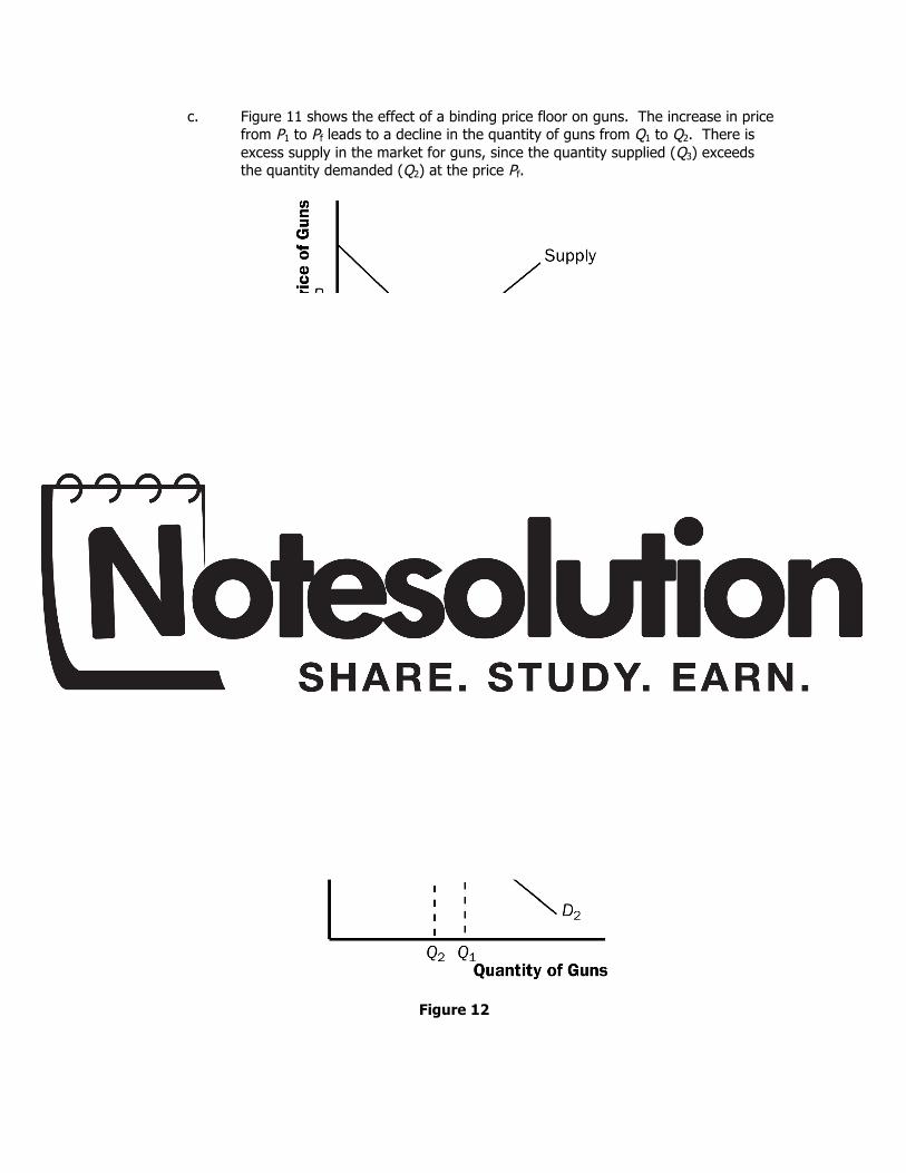
c. Figure 11 shows the effect of a binding price floor on guns. The increase in price from P1 to Pf leads to a decline in the quantity of guns from Q1 to Q2. There is excess supply in the market for guns, since the quantity supplied (Q3) exceeds the quantity demanded (Q2) at the price Pf.

Figure 11

d. Figure 12 shows the effect of a tax on ammunition. The tax on ammunition reduces the demand for guns from D1 to D2, because ammunition and guns are complements. The result is a decline in the price of guns from P1 to P2, and a decline in the quantity of guns from Q1 to Q2.

Figure 12

10. a. Programs aimed at making the public aware of the dangers of smoking reduce the demand for cigarettes, shown in Figure 13 as a shift from demand curve D1 to D2. The production quota increases the price of tobacco, which is the main ingredient in cigarettes. As a result, the supply of cigarettes shifts to the left, from S1 to S2. The effect of both programs is to reduce the quantity of cigarette consumption from Q1 to Q2.

Figure 13

b. The combined effect of the two programs on the price of cigarettes is ambiguous. The education campaign reduces demand for cigarettes, which tends to reduce the price. The tobacco production quota supports raise the cost of production of cigarettes, which tends to increase the price.

c. The taxation of cigarettes further reduces cigarette consumption, since it

increases the price to consumers. As shown in the figure, the quantity falls to Q3.

11. a. The effect of a $0.50 per cone subsidy is to shift the demand curve up by $0.50

at each quantity, since at each quantity a consumer's willingness to pay is $0.50 higher. The effects of such a subsidy are shown in Figure 14. Before the subsidy, the price is P1. After the subsidy, the price received by sellers is PS and the effective price paid by consumers is PD, which equals PS minus 50 cents. Before the subsidy, the quantity of cones sold is Q1; after the subsidy the quantity increases to Q2.

Figure 14 b. Because of the subsidy, consumers are better off, since they consume more at a

lower price. Producers are also better off, since they sell more at a higher price. The government loses, since it has to pay for the subsidy.

12. The supply of tickets is inelastic. The demand for tickets shifts downward by $5 because

of the tax. Suppose the initial equilibrium price was $75. As Figure 15 shows, the price buyers pay does not change, but the team owners lower the price by exactly $5. If the team owners did not lower the price, then the number of tickets sold would decrease, say to 15,000, and the team owners’ revenue would drop by $75×2,000=150,000; when they lower the price by $5, they sell all 17,000 seats and the revenue loss is “only” $5×17,000=$85,000. With inelastic supply, the sellers bear the entire tax burden.

Figure 15

13. a. In equilibrium, QD=QS. Replacing the expressions of demand and supply, 160�3P=140+7P. The solution to this equation is the equilibrium price, P=$2. The equilibrium quantity can be determined by replacing the price P=$2 in either the demand or the supply equation. If we use the demand equation, we get

S

Price of Hockey Tickets

D1

$75

17

D2

$70

Tax

Quantity of Hockey Tickets (thousands)

15

Q=160�3×$2=154. (Using the supply equation must give the same result.) b. With the price ceiling of $1, the quantity demanded is QD=160�3×$1=157, and

quantity supplied is QS=140+7×$1=147. There is a shortage of 157�147=10. A price ceiling of $2.5 is not binding, since the equilibrium price of $2 is lower.

c. With a price floor of $3, the quantity demanded is QD=160�3×$3=151 and the

quantity supplied is 140+7×$3=161. There is a surplus of 161�151=10. A price floor of $1.50 is not binding.

(Chapter 7) SOLUTIONS TO TEXT PROBLEMS: Quick Quizzes

1. Figure 1 shows the demand curve for turkey. The price of turkey is P1 and the consumer surplus that results from that price is denoted CS. Consumer surplus measures buyers’ willingness to pay (measured by the demand curve) minus the amount the buyers actually pay.

Figure 1

Figure 2 2. Figure 2 shows the supply curve for turkey. The price of turkey is P1 and the producer

surplus that results from that price is denoted PS. Producer surplus measures the amount sellers are paid for a good minus the sellers’ cost (measured by the supply curve).

Figure 3 3. Figure 3 shows the supply and demand for turkey. The price of turkey is P1, consumer

surplus is CS, and producer surplus is PS. Producing more turkey would lower total surplus because the value to buyers would be less than the cost to sellers.

Questions for Review 1. Buyers' willingness to pay, consumer surplus, and the demand curve are all closely

related. The height of the demand curve represents the willingness to pay of the buyers. Consumer surplus is the area below the demand curve and above the price, which equals each buyer's willingness to pay less the price of the good.

2. Sellers' costs, producer surplus, and the supply curve are all closely related. The height

of the supply curve represents the costs of the sellers. Producer surplus is the area below the price and above the supply curve, which equals the price minus each sellers' costs.

Figure 4 3. Figure 4 shows producer and consumer surplus in a supply-and-demand diagram. 4. An allocation of resources is efficient if it maximizes total surplus, the sum of consumer

surplus and producer surplus. But efficiency may not be the only goal of economic policymakers; they may also be concerned about equity⎯the fairness of the distribution of well-being.

5. The invisible hand of the marketplace guides the self-interest of buyers and sellers into

promoting general economic well-being. Despite decentralized decisionmaking and self-interested decisionmakers, free markets lead to an efficient outcome.

6. Two types of market failure are market power and externalities. Market power may

cause market outcomes to be inefficient because when firms influence prices they cause price and quantity to differ from the levels they would be under perfect competition, which keeps total surplus from being maximized. Externalities are side effects that are not taken into account by buyers and sellers. As a result, the free market does not maximize total surplus.

Problems and Applications 1. If a drought in Nova Scotia reduces the apple harvest, the supply curve for apples shifts

to the left, as shown in Figure 5. The result is a rise in the price of apples and a decline in consumer surplus from A + B + C to just A. So consumer surplus declines by the amount B + C.

Figure 5

In the market for apple juice, the higher cost of apples reduces the supply of apple juice, as shown in Figure 6. The result is a rise in the price of apple juice and a decline in consumer surplus from D + E + F to just D, a loss of E + F. Note that an event that affects consumer surplus in one market often has effects on consumer surplus in other markets.

Figure 6 2. A rise in the demand for French bread leads to an increase in producer surplus in the

market for French bread, as shown in Figure 7. The shift of the demand curve leads to an increased price, which increases producer surplus from area A to area A + B + C.

Figure 7

The increased quantity of French bread being sold increases the demand for flour, as shown in Figure 8. As a result, the price of flour rises, increasing producer surplus from area D to D + E + F. Note that an event that affects producer surplus in one market leads to effects on producer surplus in related markets.

Figure 8 3. a. Bert’s demand schedule is:

Price Quantity Demanded More than $7 0 $5 to $7 1 $3 to $5 2 $1 to $3 3 $1 or less 4

Bert’s demand curve is shown in Figure 9.

Figure 9

b. When the price of a bottle of water is $4, Bert buys two bottles of water. His consumer surplus is shown as area A in the figure. He values his first bottle of water at $7, but pays only $4 for it, so has consumer surplus of $3. He values his second bottle of water at $5, but pays only $4 for it, so has consumer surplus of $1. Thus, Bert’s total consumer surplus is $3 + $1 = $4, which is the area of A in the figure.

c. When the price of a bottle of water falls from $4 to $2, Bert buys three bottles of

water, an increase of one. His consumer surplus consists of both areas A and B in the figure, an increase in the amount of area B. He gets consumer surplus of $5 from the first bottle ($7 value minus $2 price), $3 from the second bottle ($5 value minus $2 price), and $1 from the third bottle ($3 value minus $2 price), for a total consumer surplus of $9. Thus, consumer surplus rises by $5 (which is the size of area B) when the price of a bottle of water falls from $4 to $2.

4. a. Ernie’s supply schedule for water is:

Price Quantity Supplied More than $7 4 $5 to $7 3 $3 to $5 2 $1 to $3 1 Less than $1 0

Ernie’s supply curve is shown in Figure 10.

Figure 10 b. When the price of a bottle of water is $4, Ernie sells two bottles of water. His

producer surplus is shown as area A in the figure. He receives $4 for his first bottle of water, but it costs only $1 to produce, so Ernie has producer surplus of $3. He also receives $4 for his second bottle of water, which costs $3 to produce, so he has producer surplus of $1. Thus, Ernie’s total producer surplus is $3 + $1 = $4, which is the area of A in the figure.

c. When the price of a bottle of water rises from $4 to $6, Ernie sells three bottles of water, an increase of one. His producer surplus consists of both areas A and B in the figure, an increase by the amount of area B. He gets producer surplus of $5 from the first bottle ($6 price minus $1 cost), $3 from the second bottle ($6 price minus $3 cost), and $1 from the third bottle ($6 price minus $5 price), for a total producer surplus of $9. Thus, producer surplus rises by $5 (which is the size of area B) when the price of a bottle of water rises from $4 to $6.

5. a. From Ernie’s supply schedule and Bert’s demand schedule, the quantity

demanded and supplied are:

Price Quantity Supplied Quantity Demanded $ 2 1 3

4 2 2 6 3 1

Only a price of $4 brings supply and demand into equilibrium, with an equilibrium quantity of 2.

b. At a price of $4, consumer surplus is $4 and producer surplus is $4, as shown in

problems 3 and 4. Total surplus is $4 + $4 = $8.

c. If Ernie produced one fewer bottle, his producer surplus would decline to $3, as shown in problem 4. If Bert consumed one fewer bottle, his consumer surplus would decline to $3, as shown in problem 3. So total surplus would decline to $3 + $3 = $6.

d. If Ernie produced one additional bottle of water, his cost would be $5, but the

price is only $4, so his producer surplus would decline by $1. If Bert consumed one additional bottle of water, his value would be $3, but the price is $4, so his consumer surplus would decline by $1. So total surplus declines by $1 + $1 = $2.

6. a. The effect of falling production costs in the market for flat-screen TVs results in a

shift to the right in the supply curve, as shown in Figure 11. As a result, the equilibrium price of these TVs declines and the equilibrium quantity increases.

b. The decline in the price of TVs increases consumer surplus from area A to A + B

+ C + D, an increase in the amount B + C + D. Prior to the shift in supply, producer surplus was areas B + E (the area above the supply curve and below the price). After the shift in supply, producer surplus is areas E + F + G. So producer surplus changes by the amount F + G – B, which may be positive or negative. The increase in quantity increases producer surplus, while the decline in the price reduces producer surplus. Since consumer surplus rises by B + C + D and producer surplus rises by F + G – B, total surplus rises by C + D + F + G.

c. If the supply of TVs is very elastic, then the shift of the supply curve benefits consumers most. To take the most dramatic case, suppose the supply curve were horizontal, as shown in Figure 12. Then there is no producer surplus at all. Consumers capture all the benefits of falling production costs, with consumer surplus rising from area A to area A + B.

Figure 11

Figure 12

Quantity of TVs

Demand

S1

S2

P1 P2

A

B

C

D

G

Q1 Q2

E

F

Price of TVs

Quantity of TVs

Price of TVs

S1

S2

A

B

Demand

7. Figure 13 shows supply and demand curves for haircuts. Supply equals demand at a quantity of three haircuts and a price between $4 and $5. Firms A, C, and D should cut the hair of Ricki, Jerry, and Montel. Oprah’s willingness to pay is too low and firm B’s costs are too high, so they do not participate. The maximum total surplus is the area between the demand and supply curves, which totals $11 ($8 value minus $2 cost for the first haircut, plus $7 value minus $3 cost for the second, plus $5 value minus $4 cost for the third).

Figure 13 8. a. The effect of falling production costs in the market for computers results in a

shift to the right in the supply curve, as shown in Figure 14. As a result, the equilibrium price of computers declines and the equilibrium quantity increases. The decline in the price of computers increases consumer surplus from area A to A + B + C + D, an increase in the amount B + C + D.

Figure 14

Prior to the shift in supply, producer surplus was areas B + E (the area above the supply curve and below the price). After the shift in supply, producer surplus is areas E + F + G. So producer surplus changes by the amount F + G – B, which may be positive or negative. The increase in quantity increases producer surplus, while the decline in the price reduces producer surplus. Since consumer surplus rises by B + C + D and producer surplus rises by F + G – B, total surplus rises by C + D + F + G.

Figure 15 b. Since adding machines are substitutes for computers, the decline in the price of

computers means that people substitute computers for adding machines, shifting the demand for adding machines to the left, as shown in Figure 15. The result is a decline in both the equilibrium price and equilibrium quantity of adding machines. Consumer surplus in the adding-machine market changes from area A + B to A + C, a net change of C – B. Producer surplus changes from area C + D + E to area E, a net loss of C + D. Adding machine producers are sad about technological advance in computers because their producer surplus declines.

c. Since software and computers are complements, the decline in the price and

increase in the quantity of computers means that the demand for software increases, shifting the demand for software to the right, as shown in Figure 16. The result is an increase in both the price and quantity of software. Consumer surplus in the software market changes from B + C to A + B, a net change of A – C. Producer surplus changes from E to C + D + E, an increase of C + D, so software producers should be happy about the technological progress in computers.

d. Yes, this analysis helps explain why Bill Gates is one the world’s richest men,

since his company produces a lot of software that is a complement with computers and there has been tremendous technological advance in computers.

Figure 16

9. a. Melissa’s willingness to pay is equal to $120+80=$200.

b. If the iPod was on sale for $90, Melissa’s consumer surplus would have been $200�90=$110. .

c. If the price of the iPod was $250, Melissa’s consumer surplus would have been

zero, because she wouldn’t have bought the iPod. . 10. a. The equilibrium price is given by the equation 4P�80=100�2P. The solution is

P=$30, with the corresponding quantity Q=100�2×30=40. Figure 17 shows approximately the two curves.

Figure 17

b. Consumer surplus=(1/2)(50�30)×40=400; Producer surplus =

(1/2)(30�20)×40=200. Total surplus=400+200=600. c. The buyers would bear the higher burden because they lose $400 in consumer

surplus, while the sellers lose $200.

Quantity of Broccoli

Price of Broccoli

$30

40

Supply

Demand

$50

$20

(Chapter 8) SOLUTIONS TO TEXT PROBLEMS: Quick Quizzes 1. Figure 1 shows the supply and demand curves for cookies, with equilibrium quantity Q1

and equilibrium price P1. When the government imposes a tax on cookies, the price to buyers rises to PB, the price received by sellers declines to PS, and the equilibrium quantity falls to Q2. The deadweight loss is the triangular area below the demand curve and above the supply curve between quantities Q1 and Q2. The deadweight loss shows the fall in total surplus that results from the tax.

Figure 1

2. A tax on beer would have a larger deadweight loss than a tax on milk, since the demand for beer is more elastic than the demand for milk and the deadweight loss of a tax is larger the greater is the elasticity of demand.

3. If the government doubles the tax on gasoline, the revenue from the gasoline tax could

rise or fall, depending on where the tax falls on the Laffer curve. However, if the government doubles the tax on gasoline, you can be sure that the deadweight loss of the tax rises, since deadweight loss always rises as the tax rate rises.

Questions for Review 1. When the sale of a good is taxed, both consumer surplus and producer surplus decline.

The decline in consumer surplus and producer surplus exceeds the amount of government revenue that is raised, so society's total surplus declines. The tax distorts the incentives of both buyers and sellers, so resources are allocated inefficiently.

2. Figure 2 illustrates the deadweight loss and tax revenue from a tax on the sale of a good. Without a tax, the equilibrium quantity would be Q1, the equilibrium price would be P1, consumer surplus would be A+B+C, and producer surplus would be D+E+F. The imposition of a tax places a wedge between the price buyers pay, PB, and the price sellers receive, PS, where PB = PS + tax. The quantity sold declines to Q2. Now consumer surplus is A, producer surplus is F, and government revenue is B+D. The deadweight loss of the tax is C+E, since that area is lost because of the decline in quantity from Q1 to Q2.

Figure 2 3. The greater the elasticities of demand and supply, the greater the deadweight loss of a

tax. Since elasticity measures the response of quantity to a change in price, higher elasticity means the tax induces a greater reduction in quantity, hence a greater distortion to the market.

4. Experts disagree about whether labour taxes have small or large deadweight losses

because they have different views about the elasticity of labour supply. Some believe that labour supply is inelastic, so a tax on labour has a small deadweight loss. But others think that workers can adjust their hours worked in various ways, so labour supply is elastic, and, thus, a tax on labour has a large deadweight loss.

5. The deadweight loss of a tax rises more than proportionally as the tax rises. Tax

revenue, however, may increase initially as the tax rises, but as the tax rises further, revenue eventually declines.

Problems and Applications 1. a. Figure 3 illustrates the market for pizza. The equilibrium price is P1, the

equilibrium quantity is Q1, consumer surplus is area A+B+C, and producer surplus is area D+E+F. There is no deadweight loss, as all the potential gains from trade are realized; total surplus is the entire area between the demand and supply curves⎯A+B+C+D+E+F.

Figure 3

b. With a $1 tax on each pizza sold, the price paid by buyers, PB, is now higher than the price received by sellers, PS, where PB = PS + $1. The quantity declines to Q2, consumer surplus is area A, producer surplus is area F, government revenue is area B+D, and deadweight loss is area C+E. Consumer surplus declines by B+C, producer surplus declines by D+E, government revenue increases by B+D, and deadweight loss increases by C+E.

c. If the tax were removed and consumers and producers voluntarily transferred

B+D to the government to make up for the lost tax revenue, then everyone would be better off than without the tax. The equilibrium quantity would be Q1, as in the case without the tax, and the equilibrium price would be P1. Consumer surplus would be A+C, because consumers get surplus of A+B+C, then voluntarily transfer B to the government. Producer surplus would be E+F, since producers get surplus of D+E+F, then voluntarily transfer D to the government. Both consumers and producers are better off than the case when the tax was imposed. If consumers and producers gave a little bit more than B+D to the government, then all three parties, including the government, would be better off. This illustrates the inefficiency of taxation.

2. a. The increase in demand increases the market price, as Figure 4 shows. Since the supply of land is assumed inelastic, the revenue to landlords increases.

Figure 4

b. A tax on land reduces the demand. Since the supply of land is inelastic, the

landlords have to decrease the price exactly by the amount of the tax in order to maintain the quantity demanded at the same level as the fixed amount of land supplied. The entire burden of the tax is, thus, born by the landlords. .

c. The deadweight loss is zero, because the equilibrium quantity does not change. d. George’s land tax may not apply to real estate because the supply of real estate

is not perfectly inelastic: more houses can be built when demand increases. Another difference is that real estate requires maintainance and upgrading, as opposed to unimproved land.

3. a. The statement, "A tax that has no deadweight loss cannot raise any revenue for

the government," is incorrect. An example is the case of a tax when either supply or demand is perfectly inelastic. The tax has neither an effect on quantity nor any deadweight loss, but it does raise revenue.

b. The statement, "A tax that raises no revenue for the government cannot have

any deadweight loss," is incorrect. An example is the case of a 100 percent tax imposed on sellers. With a 100 percent tax on their sales of the good, sellers won't supply any of the good, so the tax will raise no revenue. Yet the tax has a large deadweight loss, since it reduces the quantity sold to zero.

Price of Land

Quantity of Land

D2

D1

Supply

4. a. With very elastic supply and very inelastic demand, the burden of the tax on rubber bands will be borne largely by buyers. As Figure 5 shows, consumer surplus declines considerably, by area A+B, but producer surplus doesn't fall much at all, just by area C+D.

Figure 5

b. With very inelastic supply and very elastic demand, the burden of the tax on rubber bands will be borne largely by sellers. As Figure 6 shows, consumer surplus does not decline much, just by area A+B, while producer surplus falls substantially, by area C+D. Compared to part (a), producers bear much more of the burden of the tax, and consumers bear much less.

Figure 6

5. a. The deadweight loss from a tax on heating oil is likely to be greater in the fifth year after it is imposed rather than the first year. In the first year, the elasticity of demand is fairly low, as people who own oil heaters are not likely to get rid of them right away. But over time, they may switch to other energy sources and people buying new heaters for their homes will more likely choose gas or electric, so the tax will have a greater impact on quantity.

b. The tax revenue is likely to be higher in the first year after it is imposed than in

the fifth year. In the first year, demand is more inelastic, so the quantity does not decline as much and tax revenue is relatively high. As time passes and more people substitute away from oil, the equilibrium quantity declines, as does tax revenue.

6. Since the demand for food is inelastic, a tax on food is a good way to raise revenue

because it does not lead to much of a deadweight loss; thus taxing food is less inefficient than taxing other things. But it is not a good way to raise revenue from an equity point of view, since poorer people spend a higher proportion of their income on food, so the tax would hit them harder than it would hit wealthier people.

7. a. This tax has such a high rate that it is not likely to raise much revenue. Because

of the high tax rate, the equilibrium quantity in the market is likely to be at or near zero.

b. Senator Moynihan's goal was probably to ban the use of hollow-tipped bullets.

In this case, a tax is as effective as an outright ban. 8. a. Figure 7 illustrates the market for socks and the effects of the tax. Without a

tax, the equilibrium quantity would be Q1, the equilibrium price would be P1, total spending by consumers equals total revenue for producers, which is P1 x Q1, which equals area B+C+D+E+F, and government revenue is zero. The imposition of a tax places a wedge between the price buyers pay, PB, and the price sellers receive, PS, where PB = PS + tax. The quantity sold declines to Q2. Now total spending by consumers is PB x Q2, which equals area A+B+C+D, total revenue for producers is PS x Q2, which is area C+D, and government tax revenue is Q2 x tax, which is area A+B.

b. Unless supply is perfectly elastic, the price received by producers falls because of

the tax. Total receipts for producers fall, since producers lose revenue equal to area B+E+F.

Figure 7 c. The price paid by consumers rises, unless demand is perfectly elastic. Whether

total spending by consumers rises or falls depends on the price elasticity of demand. If demand is elastic, the percentage decline in quantity exceeds the percentage increase in price, so total spending declines. If demand is inelastic, the percentage decline in quantity is less than the percentage increase in price, so total spending rises. Whether total consumer spending falls or rises, consumer surplus declines because of the increase in price and reduction in quantity.

9. Since the tax on gadgets was eliminated, all tax revenue must come from the tax on

widgets. The tax revenue from the tax on widgets equals the tax per unit times the quantity produced. Assuming that neither the supply nor the demand curves for widgets are perfectly elastic or inelastic and since the increased tax causes a smaller quantity of widgets to be produced, then it is impossible for tax revenue to double--multiplying the tax per unit (which doubles) times the quantity (which declines) gives a number that is less than double the original tax revenue from widgets. So the government's tax change will yield less money than before.

10. a. The market for cola would have more elastic supply and demand curves because consumer will have access to alternative substitutes if the price of cola changes.

b. The tax rate would have to be higher for those goods which have elastic supply

and demand curves, such as cola. A marginal increase in the tax rate on all soft drinks will yield a higher tax review for government as consumers and producers are less responsive to price changes.

c. The deadweight loss of a tax would be greater, the greater the elasticities of supply and demand, in this tax, a tax on cola.

d. From a government’s point of view, the better tax would be the one placed on

the market for all soft drinks if this market faces inelastic demand and supply curves. However, it is uncertain if consumers will dramatically change their consumption of soft drinks and go to alternative substitutes such as water, coffee, tea, etc.

11. a. Tax revenue = $10×900=$9,000. The deadweight loss arises from the difference in the number of rooms rented: deadweight loss = (1/2)×$10×(1,000�900)=$500.

b. Tax revenue=$20×800=$1,600. Deadweight loss=(1/2)×$20×(1,000�800)=$2,000. Although the tax has doubled, tax revenue has increased by less than double. The increase in taxes was partially offset by the decrease in the equilibrium quantity. This result shows that the market is on the downward side of the Laffer curve.

12. Figure 8 illustrates the effects of the $2 subsidy on a good. Without the subsidy, the

equilibrium price is P1 and the equilibrium quantity is Q1. With the subsidy, buyers pay price PB, producers receive price PS (where PS = PB + $2), and the quantity sold is Q2. The following table illustrates the effect of the subsidy on consumer surplus, producer surplus, government revenue, and total surplus. Since total surplus declines by area D+H, the subsidy leads to a deadweight loss in that amount.

OLD NEW CHANGE Consumer Surplus A+B A+B+E+F+G +(E+F+G) Producer Surplus E+I B+C+E+I +(B+C) Government Revenue 0 –(B+C+D+E+F+G+H) –(B+C+D+E+F+G+H) Total Surplus A+B+E+I A+B–D+E–H+I -(D+H)

Figure 8 13. a. Setting quantity supplied equal to quantity demanded gives 2P = 300 – P.

Adding P to both sides of the equation gives 3P = 300. Dividing both sides by 3 gives P = 100. Plugging P = 100 back into either equation for quantity demanded or supplied gives Q = 200.

b. Now P is the price received by sellers and P+T is the price paid by buyers.

Equating quantity demanded to quantity supplied gives 2P = 300 - (P+T). Adding P to both sides of the equation gives 3P = 300 – T. Dividing both sides by 3 gives P = 100 - T/3. This is the price received by sellers. The buyers pay a price equal to the price received by sellers plus the tax (P+T = 100 + 2T/3). The quantity sold is now Q = 2P = 200 – 2T/3.

c. Since tax revenue is equal to T x Q and Q = 200 - 2T/3, tax revenue equals 200T - 2T2/3. Figure 9 shows a graph of this relationship. Tax revenue is zero

at T = 0 and at T = 300.

Figure 9

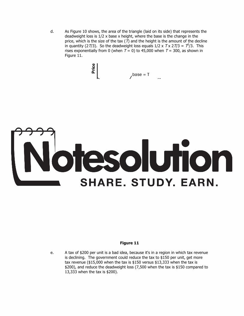
d. As Figure 10 shows, the area of the triangle (laid on its side) that represents the deadweight loss is 1/2 x base x height, where the base is the change in the price, which is the size of the tax (T) and the height is the amount of the decline in quantity (2T/3). So the deadweight loss equals 1/2 x T x 2T/3 = T2/3. This rises exponentially from 0 (when T = 0) to 45,000 when T = 300, as shown in Figure 11.

Figure 10

Figure 11

e. A tax of $200 per unit is a bad idea, because it's in a region in which tax revenue is declining. The government could reduce the tax to $150 per unit, get more tax revenue ($15,000 when the tax is $150 versus $13,333 when the tax is $200), and reduce the deadweight loss (7,500 when the tax is $150 compared to 13,333 when the tax is $200).