Chapter 2 Trends in Indian Stock Market: Scope for

Chapter 2Trends in Indian Stock Market: Scopefor Designing Profitable Trading Rule?

Abstract This chapter explores the latent structure in the Indian stock market,along with its sectors, around the financial crisis. To understand the marketstructure, the study makes use of exploratory factor analysis. It also tracks thefactor scores along with the cycles in the respective indexes to scrutinize theunderlying market behavior. Apart from looking for the latent structure, thechapter seeks to explore the following issues: How the market has behaved overthe period of study? What are the trends at sectoral level? Are they similar, orotherwise to the market trends? Are the trends independent of the selection of thestock market exchanges and whether, and how financial crisis could affect suchtrends? The rationale behind such analyses is to see whether there has been anydiscernible change in the market structure before and after the shock. A clearbehavioral pattern would hint toward an inefficient market and possible scope fordesigning profitable portfolio mix.

Keywords Indian stock market � Bombay stock exchange � National stockexchange � Stock market cycle � Structural break � Exploratory factor analysis

In the business world, the rearview mirror is always clearerthan the windshield.

Warren Buffett

2.1 Introduction

The presence of momentum trading and the resultant trial put on the efficientmarket hypothesis have attracted the attention of financial analysts and researchers.Momentum trading is a result of irrational investor behavior or ‘‘psychologicalbiases’’ or ‘‘biased self-attribution’’, and may lead to, in extreme cases, herdbehavior, formation of bubble, and subsequent panic and crashes in financialmarket. The speculative bubble generated by momentum trading inflate, becomes

G. Chakrabarti and C. Sen, Momentum Trading on the Indian Stock Market,SpringerBriefs in Economics, DOI: 10.1007/978-81-322-1127-3_2,� The Author(s) 2013

5

‘self-fulfilling’ until they eventually burst with their far-reaching, ruinous impacton real economy. The crash is usually followed by an irrational, negative bubble.Momentum trading thus leads to irrational movement in prices in both directionsand its presence is a serious attack on the myth that a capitalist system is self-regulating heading toward a stable equilibrium. Rather, as noted by Shiller andothers, it is an unstable system susceptible to ‘‘irrational exuberance’’ and ‘‘irra-tional pessimism’’.

Ours is a study that explores the possible presence of momentum trading in theIndian stock market in recent years, particularly in light of the recent global financialmelt-down of 2007–2008. Given the close connection between financial melt-downand speculative trading, the relevance of the study is obvious. The study starts withan exploration of the trend and latent structure in the Indian stock market around thecrisis and eventually tries to relate the instability to the speculative trading.

2.2 Trends and Latent Structure in Indian Stock Market

While analyzing the trends in the Indian stock market around the financial crisis of2007–2008, the study uses some benchmark stock market indexes along withdifferent sectoral indexes. The Bombay stock exchange (BSE) and the Nationalstock exchange (NSE) are the two oldest and largest stock market exchanges inIndia and hence, could be taken as representatives of the Indian stock market. Thestudy analyzes the trends, their similarities and dissimilarities, in the twoexchanges to get a complete description of Indian stock market movements. Whileanalyzing the market trends the study concentrates on the following:

How the market has behaved over the period of study. Has there been any latentstructure in the market?What are the trends at sectoral level? Are they similar, or otherwise, to the markettrends?Are the trends independent of the selection of the stock market exchanges?Whether and how financial crisis could affect the market trends?

Before we go into the detailed analysis let us briefly report on the market index andthe sectoral indexes that the study picks up from the two exchanges.The study usesdaily price data for all the market and sectoral indexes for the period ranging fromJanuary 2005 to September 2012. The price data are then used to calculate dailyreturn series using the formula Rt = ln(Pt/Pt-1), where Pt is the price on the t’th day.

2.2.1 The Market and the Sectors: Bombay Stock Exchange

The study considers BSE SENSEX or BSE Sensitive Index or BSE 30 as themarket index from BSE. BSE SENSEX, which started in January 1986 is a value-

6 2 Trends in Indian Stock Market: Scope for Designing Profitable Trading Rule?

weighted index composed of 30 largest and most actively traded stocks in BSE.The SENSEX is regarded as the pulse of the domestic stock markets in India.These companies account for around 50 % of the market capitalization of the BSE.The base value of the SENSEX is 100 on April 1, 1979, and the base year of BSE-SENSEX is 1978–1979. Initially, the index was calculated on the ‘full marketcapitalization’ method. However, it has switched to the free float method sinceSeptember 2003. The stocks represent different sectors such as, housing related,capital goods, telecom, diversified, finance, transport equipment, metal, metalproducts and mining, FMCG, information technology, power, oil and gas, andhealthcare.

As far as the sectoral indexes are concerned, we select 11 market capitalizationweighted sectoral indexes introduced by BSE in 1999. These are BSE AUTO, BSEBANKEX, BSE CD, BSE CG, BSE FMCG, BSE IT, BSE HC, BSE PSU, BSEMETAL, BSE ONG, and BSE POWER. Of these indexes, only BANKEX has itsbase year in 2000. All the others have base year in 1999 with base value of 100 inFebruary 1999. The indexes represent different sectors in the Indian economynamely, automobile, banking, consumer durables, capital goods, fast movingconsumer goods, information technology, healthcare, public sector unit, metal, oiland gas, and power, respectively.

2.2.2 The Market and the Sectors: National Stock Exchange

The NSE is the stock exchange located at Mumbai, India. In terms of marketcapitalization, it is the 11th largest index in the world. By daily turnover andnumber of trades, for both equities and derivative trading it is the largest index inIndia. NSE has a market capitalization of around US$1 trillion and over 1,652listings as of July 2012. NSE is mutually owned by a set of leading financialinstitutions, banks, insurance companies, and other financial intermediaries inIndia but its ownership and management operate as separate entities. In 2011, NSEwas the third largest stock exchange in the world in terms of the number ofcontracts traded in equity derivatives. It is the second fastest growing stockexchange in the world with a recorded growth of 16.6 %. As far as the sectoralindexes are concerned, we select some market capitalization weighted sectoralindexes introduced by NSE. These are CNX BANK, CNX COMMO, CNXENERGY, CNX FINANCE, CNX FMCG, CNX IT, CNX METALS, CNX MNC,CNX PHARMA, CNX PSU BANK, CNX PSE, CNX INFRA, and CNX SER-VICES. The indexes represent different sectors in the Indian economy namelyBank, Consumptions sector, Energy, Finance, FMCG, IT, Metal, MNC, Pharma-ceutical, Public Sector Unit, Infrastructure, and Services.

The study is conducted and market trends are analyzed over three phases in theIndian stock market:

2.2 Trends and Latent Structure in Indian Stock Market 7

1. The entire period: 2005 January to 2012 September. The trends obtained forthis entire period could be taken as the ‘average’ market trend.

2. The prologue of crisis: 2005 January to 2008 January.3. The aftermath of crisis: 2008 February to 2012 September.

The phases are constructed using the methods of detecting a structural break ina financial time series. Any financial crisis could well be thought of as a switch inregime that is often reflected in a structural break in the market volatility. In thatway, a financial crisis could possibly be associated with a volatility break orregime switches that might lead to financial crises. While identifying volatilitybreaks, we use the same methodology, introduced originally by Inclan and Tiao(1994), and used in our earlier studies (2011, 2012). We recapitulate the meth-odology briefly in the following sections.

2.3 Detection of Structural Break in Volatility

The parameters of a typical time series do not remain constant over time. It makesparadigm shifts in regular intervals. The time of this shift is the structural breakand the period between two breakpoints is known as a regime. There have beenseveral studies aimed at measuring the breakpoints. As usual, a majority of themare in the stock market. As only the algorithm used to detect the breakpoints isimportant rather than the underlying time series, the following section discussesthose studies with important breakthroughs in the algorithm.

The first group of studies was able to detect only one unknown structuralbreakpoint. Perron (1990, 1997a), Hansen (1990, 1992), Banerjee et al. (1992),Perron and Vogelsang (1992), Chu and White (1992), Andrews (1993), Andrewsand Ploberger (1994), Gregory and Hansen (1996), did some major works in thisarea. Studies by Nelson and Plosser (1982), Perron (1989), Zivot and Andrews(1992) tested unit root in presence of structural break. Bai (1994, 1997) consideredthe distributional properties of the break dates.

The second group of studies was an improvement over the first as it was able todetect multiple structural breaks in a financial time series, most importantlyendogenous breakpoints. Significant contributions were made by Zivot and Andrews(1992). Perron (1989, 1997b), Bai and Perron (2003), Lumsdaine and Papell (1997)tests for unit root allowing for two breaks in the trend function. Hansen (2001)considers multiple breaks, although he considers the breaks to be exogenously given.

The major breakthrough was the study by Inclan and Tiao (1994), who pro-posed a test to detect shifts in unconditional variance, that is, the volatility. Thistest is used extensively in financial time series to identify breaks in volatility(Wilson et al. 1996; Aggarwal et al. 1999; Huang and Yang 2001). This test waslater modified by (Sansó et al. 2004) to account for conditional variance as well.

Hsu et al. (1974) proposed in their study a model with non-stationary variancewhich is subjected to changes. This is probably the first work involving structural


breaks in variance. Hsu’s later works in 1977, 1979, and 1982 were aimed atdetecting a single break in variance in a time series. Abraham and Wei (1984)discussed methods of identifying a single structural shift in variance. Animprovement came in the study of Baufays and Rasson (1985) who addressed theissue with multiple breakpoints in their paper. Tsay (1988) also discussed ARMAmodels allowing for outliers and variance changes and proposed a method fordetecting the breakpoint in variance. More recently, Cheng (2009) provided analgorithm to detect multiple structural breakpoints for a change in mean as well asa change in variance.

This study does not explicitly incorporate any regime switching model butconsiders the period between two breaks as a regime. Schaller and Norden (1997)used Markov Switching model to find very strong evidence of regime switch inCRSP value-weighted monthly stock market returns from 1929 to 1989. Marcucci(2005) used a regime switching GARCH model to forecast volatility in S&P500which is characterized by several regime switches. Structural breaks and regimeswitch is addressed by Ismail and Isa (2006) who used a SETAR-type model to teststructural breaks in Malaysian Ringgit, Singapore Dollar, and Thai Baht.

Theoretically, volatility break dates are structural breaks in variance of a giventime series. Structural breaks are often defined as persistent and pronouncedmacroeconomic shifts in the data generating process. Usually, the probability ofobserving any structural break increases as we expand the period of study. Themethodology used in this chapter is the line of analysis followed by Inclan andTiao (1994). In the following section, we briefly recapitulate the methodology.

We may start from a simple AR(1) process as that described in (2.1)

yt ¼ aþ qyt�1 þ et

Ee2t ¼ r2

ð2:1Þ

Here et is a time series of serially uncorrelated shocks. If the series is stationary,the parameters a; q and r2 are constant over time. By definition, a structural breakoccurs if at least one of the parameters changes permanently at some point in time(Hansen 2001). The time point where the parameter changes value is often termedas a ‘‘break date’’. According to Brooks (2002), structural breaks are irreversible innature. The reasons behind occurrence of structural breaks, however, are not veryspecified. Economic and non-economic (or even unidentifiable) reasons areequally likely to bring about structural break in volatility. (Valentinyi-Endrész2004).

2.3.1 Detection of Multiple Structural Breaks in Variance:The ICSS Test

The Iterative Cumulative Sum of Squares (or the ICSS) algorithm by Inclan andTiao (1994) can very well detect sudden changes in unconditional variance for a

2.3 Detection of Structural Break in Volatility 9

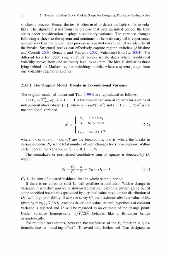
stochastic process. Hence, the test is often used to detect multiple shifts in vola-tility. The algorithm starts from the premise that over an initial period, the timeseries under consideration displays a stationary variance. The variance changesfollowing a shock to the system and continues to be stationary till it experiencesanother shock in the future. This process is repeated over time till we identify allthe breaks. Structural breaks can effectively capture regime switches (Altissimoand Corradi 2003; Gonzalo and Pitarakis 2002; Valentinyi-Endrész 2004). Thedifferent tests for identifying volatility breaks isolate dates where conditionalvolatility moves from one stationary level to another. The idea is similar to thoselying behind the Markov regime switching models, where a system jumps fromone volatility regime to another.

2.3.1.1 The Original Model: Breaks in Unconditional Variance

The original model of Inclan and Tiao (1994) are reproduced as follows:

Let Ck ¼Pk

t¼1 a2t ; k ¼ 1; . . .;T is the cumulative sum of squares for a series of

independent observations atf g, where at � iidN 0; r2ð Þ and t = 1, 2, …, T, r2 is theunconditional variance.

r2 ¼

s0; 1\t\j1

s1; j1\t\j2

. . .sNT ; jNT \t\T

8>><

>>:ð2:2Þ

where 1\j1\j2\ � � � jNT \T are the breakpoints, that is, where the breaks invariances occur. NT is the total number of such changes for T observations. Withineach interval, the variance is s2

j ; j ¼ 0; 1; . . .;NT

The centralized or normalized cumulative sum of squares is denoted by Dk

where

Dk ¼Ck

CT� k

T! D0 ¼ DT ¼ 0 ð2:3Þ

CT is the sum of squared residuals for the whole sample period.If there is no volatility shift Dk will oscillate around zero. With a change in

variance, it will drift upward or downward and will exhibit a pattern going out ofsome specified boundaries (provided by a critical value based on the distribution ofDk) with high probability. If at some k, say k*, the maximum absolute value of Dk,

given by maxk

ffiffiffiffiffiffiffiffiffiffiffiffiffiffiT=2Dk

p��

�� exceeds the critical value, the null hypothesis of constant

variance is rejected and k* will be regarded as an estimate of the change point.

Under variance homogeneity,ffiffiffiffiffiffiffiffiffiffiffiffiffiffiT=2Dk

pbehaves like a Brownian bridge

asymptotically.For multiple breakpoints, however, the usefulness of the Dk function is ques-

tionable due to ‘‘masking effect’’. To avoid this, Inclan and Tiao designed an


iterative algorithm that uses successive application of the Dk function at differentpoints in the time series to look for possible shift in volatility.

2.3.1.2 Modified ICSS Test: Breaks in Conditional Variance

The modified ICSS test is reproduced and used in this study. Sansó et al. (1994)found significant size distortions for the ICSS test in presence of excessive kurtosisand conditional heteroscedasticity. This makes original ICSS test invalid in thecontext of financial time series that are often characterized by fat tails and con-ditional heteroscedasticity. As a remedial measure, they introduced two tests toexplicitly consider the fourth moment properties of the disturbances and theconditional heteroscedasticity.

The first test, or the k1 test, makes the asymptotic distribution free of nuisanceparameters for iid zero mean random variables.

j1 ¼ supk T�1=2Bk

��

��; k¼ 1;. . .;T

Bk ¼Ck � k

T CTffiffiffiffiffiffiffiffiffiffiffiffiffiffiffin4 � r4p ; g4 ¼ T�1

XT

t¼1

e4t and r4 ¼ T�1CT

ð2:4Þ

This statistic is free of any nuisance parameter. The second test, the j2 testsolves the problems of fat tails and persistent volatility.

j2 ¼ supk T�1=2Gk

��

�� ð2:5Þ

where Gk ¼ x�1

24 ðCk � k

T CTÞx4 is a consistent estimator of x4. A nonparametric estimator of x4 can be

expressed as

x4 ¼1T

XT

i¼1

ðe2t � r2Þ2 þ 2

T

Xm

l¼1

xðl;mÞXT

t¼1

ðe2t � r2Þðe2

t�1 � r2Þ ð2:6Þ

xðl;mÞ is a lag window, such as Bartlett and defined as xðl;mÞ ¼ 1� l= mþ 1ð Þ½ �:The bandwidth m is chosen by Newey-West (1994) technique. The j2 test is morepowerful than the original Inclan-Tiao test or even the j1test and is best fit for ourpurpose.

The use of the above-mentioned tests on our data set identifies the sub-phasesmentioned earlier. One point, however, is to be noted while considering these sub-phases. The period of aftermath might be found to be characterized by furtherfluctuations in the Indian stock market, some of which might even be capable ofgenerating further financial market crisis. However, analysts often consider it tooearly to call this period another era of financial crisis. This period of financialturmoil and vulnerability should be better treated as aftershocks of the crisis of2007–2008 than altogether a new eon of crisis. Moreover, the fluctuations in recentyears are yet to be comparable to the older ones in terms of their overall

2.3 Detection of Structural Break in Volatility 11

devastating impact on the real economy. Our study hence is built particularlyaround the financial crisis of 2007–2008. And hence, the crisis period and itsaftermath are exclusively in terms of this financial crisis.

2.4 Identifying Trends in Indian Stock Market:The Methodology

The latent structure in the market could be best analyzed by using an exploratoryfactor analysis (EFA). EFA is a simple, nonparametric method for extractingrelevant information from large correlated data sets (Hair et al. 2010). It couldreduce a complex data set to a lower dimension to reveal the sometimes hidden,simplified structures that often underlie it. In EFA, each variable (Xi) is expressedas a linear combination of underlying factors (Fi). The amount of variance eachvariable shares with others is called communality. The covariance among variablesis described by common factors and a unique factor (Ui) for each variable. Hence,

Xi ¼ Ai1F1 þ � � � þ AimFm þ ViUi ð2:7Þ

and Fi ¼ Wi1X1 þ � � � þ WikXk ð2:8Þ

where, Ai1is the standardized multiple regression coefficient of variable i on factorj; Vi is the standardized regression coefficient of variable i on unique factor i; m isthe number of common factors; Wi’s are the factor scores, and k is the number ofvariables. The unique factors are uncorrelated with each other and with commonfactors.

The appropriateness of using EFA on a data set could be judged by Bartlett’stest of sphericity and the Kaiser-Meyar-Olkin (KMO) measure. The Bartlett’s testof sphericity tests the null of population correlation matrix to be an identity matrix.A statistically significant Bartlett statistic indicates the extent of correlation amongvariables to be sufficient to use EFA. Moreover, KMO measure of samplingadequacy should exceed 0.50 for appropriateness of EFA.

In factor analysis, the variables are grouped according to their correlation sothat variables under a particular factor are strongly correlated with each other.When variables are correlated they will share variances among them. A variable’scommunality is the estimate of its shared variance among the variables representedby a specific factor.

Through appropriate methods, factor scores could be selected so that the firstfactor explains the largest portion of the total variance. Then a second set,uncorrelated to the first, could be found so that the second factor accounts for mostof the residual variance and so on. This chapter uses the Principal Componentmethod where the total variance in data is considered. The method helps when weisolate minimum number of factors accounting for maximum variance in data.


Factors with eigenvalues greater than 1.0 are retained. An eigenvalue representsthe amount of variance associated with the factor. Factors with eigenvalues lessthan one are not better than a single variable, because after standardization, eachvariable has a variance of 1.0.

Interpretation of factors will require an examination of the factor loadings. Afactor loading is the correlation of the variable and the factor. Hence, the squaredloading is the variable’s total variance accounted by the factor. Thus, a 0.50loading implies that 25 % of the variance of the variable is explained by the factor.Usually, factor loadings in the range of ±0.30 to ±0.40 are minimally required forinterpretation of a structure. Loadings greater than or equal to ±0.50 are practi-cally significant while loadings greater than or equal to ±0.70 imply presence ofwell-defined structures.

The initial or unrotated factor matrix, however, shows the relationship betweenthe factors and the variables where factor solutions extract factors in the order oftheir variance extracted. The first factor accounting for the largest amount ofvariance in the data is a general factor where almost every variable has significantloading. The subsequent factors are based on the residual amount of variance. Suchfactors are difficult to interpret as a single factor could be related to many vari-ables. Factor rotation provides simpler factor structures that are easier to interpret.With rotation, the reference axes of the factors are rotated about the origin, untilsome other positions are reached. With factor rotation, variance is re-distributedfrom the earlier factor to the latter. Effectively, one factor will be significantlycorrelated with only a few variables and a single variable will have high andsignificant loading with only one factor. In an orthogonal factor rotation, as theaxes are maintained at angles of 90�, the resultant factors will be uncorrelated toeach other. Within the orthogonal factor rotation methods, VARIMAX is the mostpopular method where the sum of variances of the required loading of the factormatrix is maximized. There are, however, oblique factor rotations where the ref-erence axes are not maintained at 90� angles. The resulting factors will not betotally uncorrelated to each other. This chapter will use that method of factorrotation which will fit the data best.

The study then employs Cronbach’s alpha as a measure of internal consistency.In theory a high value of alpha is often used as evidence that the items measure anunderlying (or latent) construct. Cronbach’s alpha, however, is not a statistical test.It is a coefficient of reliability or consistency.

The standardized Cronbach’s alpha could be written as: a ¼ N:�c�vþ N�1ð Þ:�c

Here N is the number of items (here markets); c is the average inter-itemcovariance among the items and v is the average variance. From the formula, it isclear that an increase in the number of items increases Cronbach’s alpha. Addi-tionally, if the average inter-item correlation increases, Cronbach’s alpha increasesas well (holding the number of items constant). This study uses Cronbach’s alphato check how closely related a set of markets are as a group and whether theyindeed form a ‘group’ among themselves.

2.4 Identifying Trends in Indian Stock Market: The Methodology 13

2.5 Trends and Latent Structure in Indian Stock Market:Bombay Stock Exchange

1. Trends over the entire period: 2005 January to 2012 September

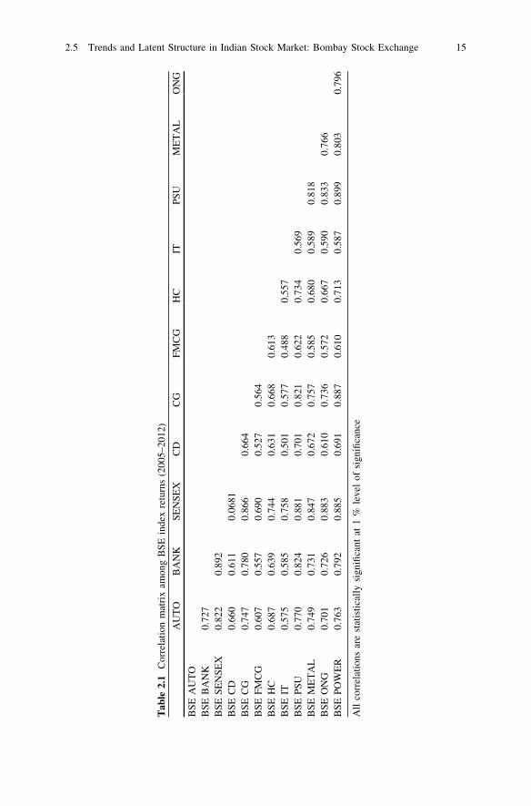
The study starts from an analysis of correlation among the different indexes.Table 2.1 suggests presence of statistically significant correlation among market aswell as sectoral returns over the entire study period.

To justify the use of EFA over the chosen data set we consider the KMO andBartlett’s tests for data adequacy. The KMO measure of sampling adequacy takesa value of 0.873 and Bartlett’s test statistic of sphericity is significant at onepercent level of significance implying validity of using EFA on our data set.

Based on eigenvalue a single factor (eigenvalue 8.784) is extracted thatexplains 73.2 % of total variability. The single factor contains all the indexes thatare highly loaded in that factor. The Cronbach’s alpha stands at 0.9631 anddeclines with exclusion of each index. This makes the extracted structure a validone (Table 2.2).

The presence of a single structure implies the presence of a single dominanttrend in the market. All the sectors and the market move in similar fashion anddirection (as reflected in their positive loadings on the factor). The indexes arehighly correlated and together they reflect a distinct and broad market trend. Thedetailed analysis of such broad, dominant trend could be of further interest.

Analysis of market trend: use of factor scoreIn EFA, factors represent latent constructs. From a practical standpoint,

researchers often estimate scores on a latent construct (i.e., factor scores) and usethem instead of the set of items that load on that factor. While constructing a factorscore, researchers could use the sum or average of the scores on items loading onthat factor. However, the procedure could be refined and made statisticallyacceptable by using the information contained in the factor solution. The problemwith such elementary construction of factor score is that simple average uses onlythe information that the set of items load on a given factor. The process fails ifitems have different loadings on the factor. In such cases, some items, with rela-tively high loadings, are better measures of the underlying factor (i.e., more highlycorrelated with the factor) than others. Therefore, construction of ‘good’ factorscores requires attaching higher weights to items with high loadings and viceversa. The weights that are used to combine scores on observed items to formfactor scores could be obtained through some form of least squares regression.Thus, the factor scores obtained serve as estimates of their corresponding unob-served counterparts.

The use of EFA on our data set extracts a single factor that could be thought ofas representing the broad trend in the stock market. However, the stock markettrend could not be properly or effectively analyzed until and unless we could getsome proxy for this trend. Individual items in the factors (the market index and allthe sectoral indexes) could be analyzed separately but the process will provide us


Tab

le2.

1C

orre

lati

onm

atri

xam

ong

BS

Ein

dex

retu

rns

(200

5–20

12)

AU

TO

BA

NK

SE

NS

EX

CD

CG

FM

CG

HC

ITP

SU

ME

TA

LO

NG

BS

EA

UT

OB

SE

BA

NK

0.72

7B

SE

SE

NS

EX

0.82

20.

892

BS

EC

D0.

660

0.61

10.

0681

BS

EC

G0.

747

0.78

00.

866

0.66

4B

SE

FM

CG

0.60

70.

557

0.69

00.

527

0.56

4B

SE

HC

0.68

70.

639

0.74

40.

631

0.66

80.

613

BS

EIT

0.57

50.

585

0.75

80.

501

0.57

70.

488

0.55

7B

SE

PS

U0.

770

0.82

40.

881

0.70

10.

821

0.62

20.

734

0.56

9B

SE

ME

TA

L0.

749

0.73

10.

847

0.67

20.

757

0.58

50.

680

0.58

90.

818

BS

EO

NG

0.70

10.

726

0.88

30.

610

0.73

60.

572

0.66

70.

590

0.83

30.

766

BS

EP

OW

ER

0.76

30.

792

0.88

50.

691

0.88

70.

610

0.71

30.

587

0.89

90.

803

0.79

6

All

corr

elat

ions

are

stat

isti

call

ysi

gnifi

cant

at1

%le

vel

ofsi

gnifi

canc

e

2.5 Trends and Latent Structure in Indian Stock Market: Bombay Stock Exchange 15

with hardly any insight regarding the broad trend. We could instead construct thefactor score for our single extracted factor. These factor scores then could serve asa proxy for the latent structure of the market. That is where the study moves next.

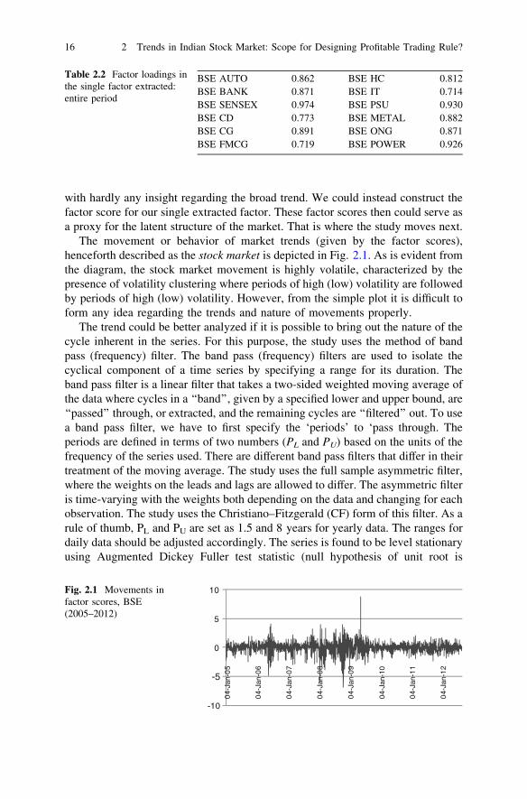
The movement or behavior of market trends (given by the factor scores),henceforth described as the stock market is depicted in Fig. 2.1. As is evident fromthe diagram, the stock market movement is highly volatile, characterized by thepresence of volatility clustering where periods of high (low) volatility are followedby periods of high (low) volatility. However, from the simple plot it is difficult toform any idea regarding the trends and nature of movements properly.

The trend could be better analyzed if it is possible to bring out the nature of thecycle inherent in the series. For this purpose, the study uses the method of bandpass (frequency) filter. The band pass (frequency) filters are used to isolate thecyclical component of a time series by specifying a range for its duration. Theband pass filter is a linear filter that takes a two-sided weighted moving average ofthe data where cycles in a ‘‘band’’, given by a specified lower and upper bound, are‘‘passed’’ through, or extracted, and the remaining cycles are ‘‘filtered’’ out. To usea band pass filter, we have to first specify the ‘periods’ to ‘pass through. Theperiods are defined in terms of two numbers (PL and PU) based on the units of thefrequency of the series used. There are different band pass filters that differ in theirtreatment of the moving average. The study uses the full sample asymmetric filter,where the weights on the leads and lags are allowed to differ. The asymmetric filteris time-varying with the weights both depending on the data and changing for eachobservation. The study uses the Christiano–Fitzgerald (CF) form of this filter. As arule of thumb, PL and PU are set as 1.5 and 8 years for yearly data. The ranges fordaily data should be adjusted accordingly. The series is found to be level stationaryusing Augmented Dickey Fuller test statistic (null hypothesis of unit root is

Table 2.2 Factor loadings inthe single factor extracted:entire period

BSE AUTO 0.862 BSE HC 0.812BSE BANK 0.871 BSE IT 0.714BSE SENSEX 0.974 BSE PSU 0.930BSE CD 0.773 BSE METAL 0.882BSE CG 0.891 BSE ONG 0.871BSE FMCG 0.719 BSE POWER 0.926

-10

-5

0

5

10

04-

Jan-

05

04-

Jan-

06

04-

Jan-

07

04-

Jan-

08

04-

Jan-

09

04-J

an-1

0

04-

Jan-

11

04-

Jan-

12

Fig. 2.1 Movements infactor scores, BSE(2005–2012)


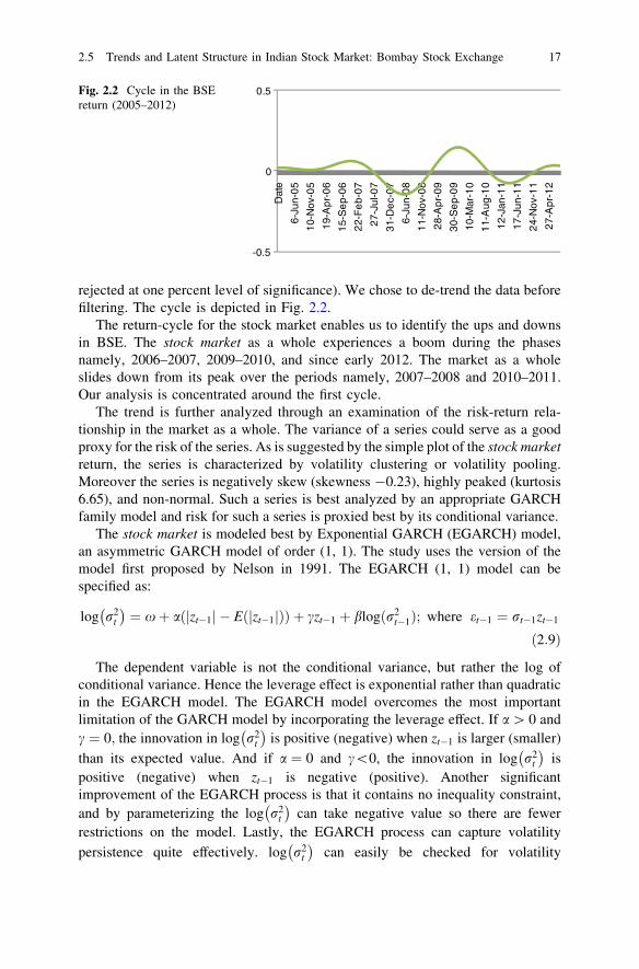
rejected at one percent level of significance). We chose to de-trend the data beforefiltering. The cycle is depicted in Fig. 2.2.

The return-cycle for the stock market enables us to identify the ups and downsin BSE. The stock market as a whole experiences a boom during the phasesnamely, 2006–2007, 2009–2010, and since early 2012. The market as a wholeslides down from its peak over the periods namely, 2007–2008 and 2010–2011.Our analysis is concentrated around the first cycle.

The trend is further analyzed through an examination of the risk-return rela-tionship in the market as a whole. The variance of a series could serve as a goodproxy for the risk of the series. As is suggested by the simple plot of the stock marketreturn, the series is characterized by volatility clustering or volatility pooling.Moreover the series is negatively skew (skewness -0.23), highly peaked (kurtosis6.65), and non-normal. Such a series is best analyzed by an appropriate GARCHfamily model and risk for such a series is proxied best by its conditional variance.

The stock market is modeled best by Exponential GARCH (EGARCH) model,an asymmetric GARCH model of order (1, 1). The study uses the version of themodel first proposed by Nelson in 1991. The EGARCH (1, 1) model can bespecified as:

log r2t

� �¼ xþ a zt�1j j � E zt�1j jð Þð Þ þ czt�1 þ blogðr2

t�1Þ; where et�1 ¼ rt�1zt�1

ð2:9Þ

The dependent variable is not the conditional variance, but rather the log ofconditional variance. Hence the leverage effect is exponential rather than quadraticin the EGARCH model. The EGARCH model overcomes the most importantlimitation of the GARCH model by incorporating the leverage effect. If a [ 0 andc ¼ 0; the innovation in log r2

t

� �is positive (negative) when zt�1 is larger (smaller)

than its expected value. And if a ¼ 0 and c\0, the innovation in log r2t

� �is

positive (negative) when zt�1 is negative (positive). Another significantimprovement of the EGARCH process is that it contains no inequality constraint,and by parameterizing the log r2

t

� �can take negative value so there are fewer

restrictions on the model. Lastly, the EGARCH process can capture volatility

persistence quite effectively. log r2t

� �can easily be checked for volatility

-0.5

0

0.5

Dat

e

6-Ju

n-0

5

10-

Nov

-05

19-

Apr

-06

15-

Se

p-0

6

22-

Fe

b-0

7

27-

Jul-0

7

31-

De

c-0

7

6-Ju

n-0

8

11-

Nov

-08

28-

Apr

-09

30-

Se

p-0

9

10-

Mar

-10

11-

Aug

-10

12-

Jan-

11

17-

Jun-

11

24-

Nov

-11

27-

Apr

-12

Fig. 2.2 Cycle in the BSEreturn (2005–2012)


persistence by looking at the stationarity and ergodicity conditions. However, theEGARCH model is also not free from its drawbacks. This model is difficult to usefor there is no analytic form for the volatility term structure.

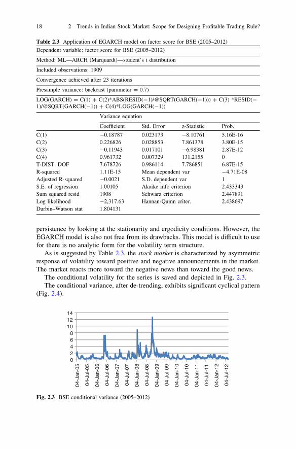
As is suggested by Table 2.3, the stock market is characterized by asymmetricresponse of volatility toward positive and negative announcements in the market.The market reacts more toward the negative news than toward the good news.

The conditional volatility for the series is saved and depicted in Fig. 2.3.The conditional variance, after de-trending, exhibits significant cyclical pattern

(Fig. 2.4).

Table 2.3 Application of EGARCH model on factor score for BSE (2005–2012)

Dependent variable: factor score for BSE (2005–2012)

Method: ML—ARCH (Marquardt)—student’s t distribution

Included observations: 1909

Convergence achieved after 23 iterations

Presample variance: backcast (parameter = 0.7)

LOG(GARCH) = C(1) ? C(2)*ABS(RESID(-1)/@SQRT(GARCH(-1))) ? C(3) *RESID(-1)/@SQRT(GARCH(-1)) ? C(4)*LOG(GARCH(-1))

Variance equation

Coefficient Std. Error z-Statistic Prob.

C(1) -0.18787 0.023173 -8.10761 5.16E-16C(2) 0.226826 0.028853 7.861378 3.80E-15C(3) -0.11943 0.017101 -6.98381 2.87E-12C(4) 0.961732 0.007329 131.2155 0T-DIST. DOF 7.678726 0.986114 7.786851 6.87E-15R-squared 1.11E-15 Mean dependent var -4.71E-08Adjusted R-squared -0.0021 S.D. dependent var 1S.E. of regression 1.00105 Akaike info criterion 2.433343Sum squared resid 1908 Schwarz criterion 2.447891Log likelihood -2,317.63 Hannan-Quinn criter. 2.438697Durbin–Watson stat 1.804131

02468

101214

04-

Jan-

05

04-

Jul-0

5

04-

Jan-

06

04-

Jul-0

6

04-

Jan-

07

04-

Jul-0

7

04-

Jan-

08

04-

Jul-0

8

04-

Jan-

09

04-

Jul-0

9

04-

Jan-

10

04-

Jul-1

0

04-

Jan-

11

04-

Jul-1

1

04-

Jan-

12

04-

Jul-1

2

Fig. 2.3 BSE conditional variance (2005–2012)


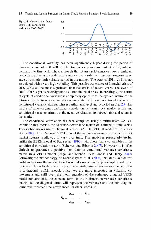
The conditional volatility has been significantly higher during the period offinancial crisis of 2007–2008. The two other peaks are not at all significantcompared to this peak. Thus, although the return cyclebrings out two significantpeaks in BSE return, conditional variance cycle rules out one and suggests pres-ence of a single high-volatile period in the market. The peak of 2010–2011 is notassociated with a very high volatility. This justifies our choice of financial crisis of2007–2008 as the most significant financial crisis of recent years. The cycle of2010–2012 is yet to be designated as a true financial crisis. Interestingly, the natureof cycle of conditional variance is completely opposite to the cyclical nature of thereturn series. Return peaks are always associated with low conditional variance orconditional variance slumps. This is further analyzed and depicted in Fig. 2.4. Thenature of time-varying conditional correlation between stock market return andconditional variance brings out the negative relationship between risk and return inthe market.

The conditional correlation has been computed using a multivariate GARCHtechnique that models the variance–covariance matrix of a financial time series.This section makes use of Diagonal Vector GARCH (VECH) model of Bollerslevet al. (1988). In a Diagonal VECH model the variance–covariance matrix of stockmarket returns is allowed to vary over time. This model is particularly useful,unlike the BEKK model of Baba et al. (1990), with more than two variables in theconditional correlation matrix (Scherrer and Ribarits 2007). However, it is oftendifficult to guarantee a positive semi-definite conditional variance–covariancematrix in a VECH model (Engel and Kroner 1993; Brooks and Henry 2000).Following the methodology of Karunanayake et al. (2008) this study avoids thisproblem by using the unconditional residual variance as the pre-sample conditionalvariance. This is likely to ensure positive semi-definite variance–covariance matrixin a diagonal VECH model. Since, we are more interested in volatility co-movement and spill over, the mean equation of the estimated diagonal VECHmodel contains only the constant term. In the n dimension variance–covariancematrix, H, the diagonal terms will represent the variance and the non-diagonalterms will represent the covariances. In other words, in

Ht ¼h11t � � � h1nt

� � � � � � � � �hn1t � � � hnnt

-1

-0.5

0

0.5

1

1.5

6-Ju

n-0

5

10-

Nov

-05

19-

Apr

-06

15-

Se

p-0

6

22-

Fe

b-0

7

27-

Jul-0

7

31-

De

c-0

7

6-Ju

n-0

8

11-

Nov

-08

28-

Apr

-09

30-

Se

p-0

9

10-

Mar

-10

11-

Aug

-10

12-

Jan-

11

17-

Jun-

11

24-

Nov

-11

27-

Apr

-12

Fig. 2.4 Cycle in the factorscore BSE conditionalvariance (2005–2012)


hiit is the conditional variance of ‘ith market in time t; hijt is the conditionalcovariance between the ith and jth market in period t (i = j). The conditionalvariance depends on the squared lagged residuals and conditional covariancedepends on the cross lagged residuals and lagged covariances of the other series(Karunanayake et al. 2008). The model could be represented as:

VECH Htð Þ ¼ C þ A:VECHðet�1e0t�1Þ þ B:VECH Ht�1ð Þ ð2:10Þ

A and B are N Nþ1ð Þ2 � N Nþ1ð Þ

2 parameter matrices. C is N Nþ1ð Þ2 vector of constant.

aii in matrix A, that is the diagonal elements show the own spillover effect. This isthe impact of own past innovations on present volatility. The cross diagonal terms(aij; i 6¼ j) show the impact of pat innovation in one market on the present vola-tility of other markets. Similarly, bii in matrix B shows the impact of own pastvolatility on present volatility. Likewise, bij represents cross volatility spill over orthe impact of past volatility of the ith market on the present volatility of jth market.For our purpose, aij’s and bij’s are more important.

As pointed out by Karunanayake et al. (2008) an important issue in estimating adiagonal VECH model is the number of parameters to be estimated. To solve theproblem, Bollerslev et al. (1988) suggested use of a diagonal form of A and B. Arelated issue is to ensure the positive semi-definiteness of the variance–covariancematrix. The condition is easily satisfied if all of the parameters in A, B, and C arepositive with a positive initial conditional variance–covariance matrix. Bollerslevet al. (1988) suggested some restrictions to impose that have been followed byKarunanayake et al. (2008). They used maximum likelihood function to generatethese parameter estimates by imposing some restriction on the initial value. If h bethe parameter for a sample of T observations, the log likelihood function will be:

T hð Þ ¼XT

t¼1

lr hð Þ; where lt hð Þ ¼ N

2ln 2pð Þ � 1

2ln Htj j �

12�0tH

�1t �t ð2:11Þ

The presample values of h can be set to be equal to their expected value of zero(Bollerslev et al. 1988). The Ljung Box test statistic could further be used to testfor remaining ARCH effects. For a stationary time series of T observations and amultivariate process of order (p, q) the Ljung Box test statistic is given as:

Q ¼ T2Xs

j¼1

ðT � jÞ�1tj C�1Ytð0ÞCYtðjÞC�1

Ytð0ÞC0Yt

ðjÞn

ð2:12Þ

Yt is VECH (yt, y0t), CYtðjÞ is the sample autocovariance matrix of order j, s isthe number of lags used, T is the number of observations. For large sample, the teststatistic is distributed as a v2 under the null hypothesis of no remaining ARCHeffect.

A multivariate GARCH of appropriate order has been estimated for the data onfactor scores for BSE return and BSE conditional variance and the conditionalcorrelation values have been saved. The movement in this conditional correlation


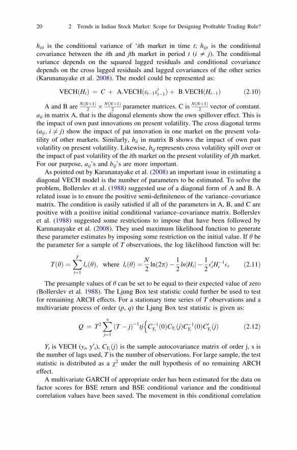
reflects the risk-return relationship in the context of BSE. During most of the timeperiod, particularly during the financial crisis of 2007–2008, risk and return hadbeen perfectly negatively correlated (correlation coefficient = -1). For only ashort period of time, risk and return was perfectly positively correlated (correlationcoefficient = +1). This suggests the presence of dominantly negative (perfect)risk-return relationship in BSE. More interestingly, correlation coefficient waseither +1 or -1. Only for a short period of time (during August 2010 to January2012) correlation coefficient remained positive and fluctuated. The characteristicsin conditional correlation could further be traced in the cycle in conditional cor-relation (Fig. 2.5).

The analysis of overall market trend would now be supplemented by analysesof market trend before and after the crisis.

2. The trends in the pre-crisis period: 2005 January to 2008 January

The analysis of trends in the market in the pre-crisis period starts from iden-tification of latent structure in the market.

Table 2.4 suggests presence of statistically significant correlation among mar-ket as well as sectoral returns during the pre-crisis.The correlation coefficients aremore or less the same in magnitude compared to those for the entire period.

The use of EFA over the pre-crisis data set is further justified by the favorablevalues of the KMO measure of sampling adequacy and Bartlett’s tests for dataadequacy. The KMO measure of sampling adequacy takes a value of 0.885 andBartlett’s test statistic of sphericity is significant at one percent level of signifi-cance implying validity of using EFA on the pre-crisis data set.

On the basis of eigenvalue a single factor (eigenvalue 8.908) is extracted thatexplains 74.2 % of total variability. Both the eigenvalue and the total variabilityexplained by the single factor extracted are higher than those obtained for theentire period. Once again, the single factor contains all the indexes that are highlyloaded in that factor. The Cronbach’s alpha stands at 0.9650 (which is higher thanthe entire period) and declines with exclusion of each index. This makes theextracted structure, once again a valid one (Table 2.5).

-1

-0.5

0

0.5

1

1.5

Dat

e

2-A

ug-0

5

7-M

ar-0

6

5-O

ct-0

6

14-

May

-07

7-D

ec-

07

14-

Jul-0

8

19-

Fe

b-0

9

29-

Se

p-0

9

7-M

ay-1

0

2-D

ec-

10

5-Ju

l-11

7-F

eb-

12

CYCLE_MARKET

CYCLE_CON_VAR

CYCLE_COND_COR

Fig. 2.5 Return-risk relationship BSE (2005–2012)


Tab

le2.

4C

orre

lati

onm

atri

xam

ong

BS

Ein

dex

retu

rns

(200

5–20

08)

AU

TO

BA

NK

SE

NS

EX

CD

CG

FM

CG

HC

ITP

SU

ME

TA

LO

NG

BS

EA

UT

OB

SE

BA

NK

0.69

3B

SE

SE

NS

EX

0.85

70.

842

BS

EC

D0.

691

0.54

10.

656

BS

EC

G0.

769

0.69

30.

850

0.63

3B

SE

FM

CG

0.68

60.

562

0.75

30.

569

0.63

8B

SE

HC

0.76

00.

659

0.80

20.

670

0.72

40.

670

BS

EIT

0.65

00.

572

0.78

50.

507

0.60

60.

495

0.60

6B

SE

PS

U0.

812

0.79

40.

897

0.69

20.

812

0.68

50.

787

0.61

0B

SE

ME

TA

L0.

765

0.67

30.

837

0.64

80.

752

0.66

30.

728

0.59

20.

834

BS

EO

NG

0.74

70.

678

0.87

60.

612

0.72

80.

657

0.71

80.

603

0.86

90.

760

BS

EP

OW

ER

0.78

00.

716

0.85

50.

660

0.86

70.

652

0.75

00.

588

0.89

40.

794

0.78

3

All

corr

elat

ions

are

stat

isti

call

ysi

gnifi

cant

at1

%le

vel

ofsi

gnifi

canc

e


The presence of a single structure implies the presence of a single dominanttrend in the market even in the pre-crisis period. All the sectors and the marketmove in similar fashion and direction (as reflected in their positive loadings on thefactor). The indexes are highly correlated and together they reflect a distinct andbroad market trend. The detailed analysis of such broad, dominant trend in the pre-crisis period would be our further area of analysis.

Analysis of market trend in pre-crisis period: use of factor scoreThe use of EFA on our pre-crisis data set extracts a single factor that could be

thought of as representing the broad trend in the stock market in the pre-crisisperiod. However, this stock market trend cannot be properly or effectively ana-lyzed until and unless we could get some proxy for this trend. Just like the previouscase, we have constructed the factor score for our single extracted factor for thepre-crisis period. These factor scores then serve as a proxy for the latent structureof the pre-crisis market.

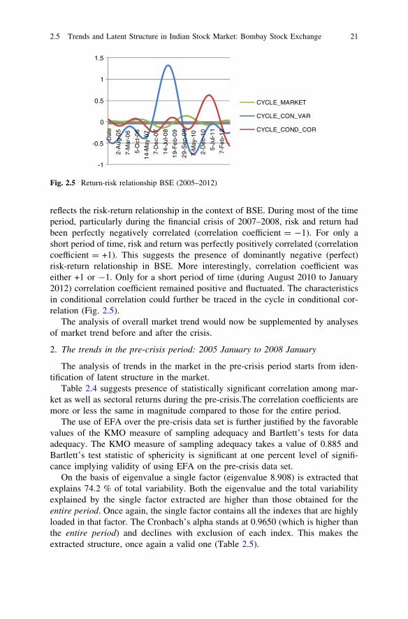
The movement or behavior of market trends (given by the factor scores),henceforth described as the stock market in pre-crisis period, is depicted inFig. 2.6. As is evident from the diagram, the stock market movement is highlyvolatile, characterized by the presence of volatility clustering where periods ofhigh (low) volatility are followed by periods of high (low) volatility. However,from the simple plot it is difficult to form any idea regarding the trends and natureof movements properly. The trend in the pre-crisis period resembles that for theentire Period.

The trend could be better analyzed if it is possible to bring out the nature of thecycle inherent in the series. The cycle is generated once again using the method ofband pass (frequency) filter in its CF form. The pre-crisis series is found to belevel stationary using Augmented Dickey Fuller test statistic (null hypothesis ofunit root is rejected at one percent level of significance). We chose to de-trend thedata before filtering. The cycle is depicted in Fig. 2.7.

Table 2.5 Factor loadings inthe single factor extracted:pre-crisis period


-8

-6

-4

-2

0

2

4

6

04-Jan-05 04-Jan-06 04-Jan-07 04-Jan-08



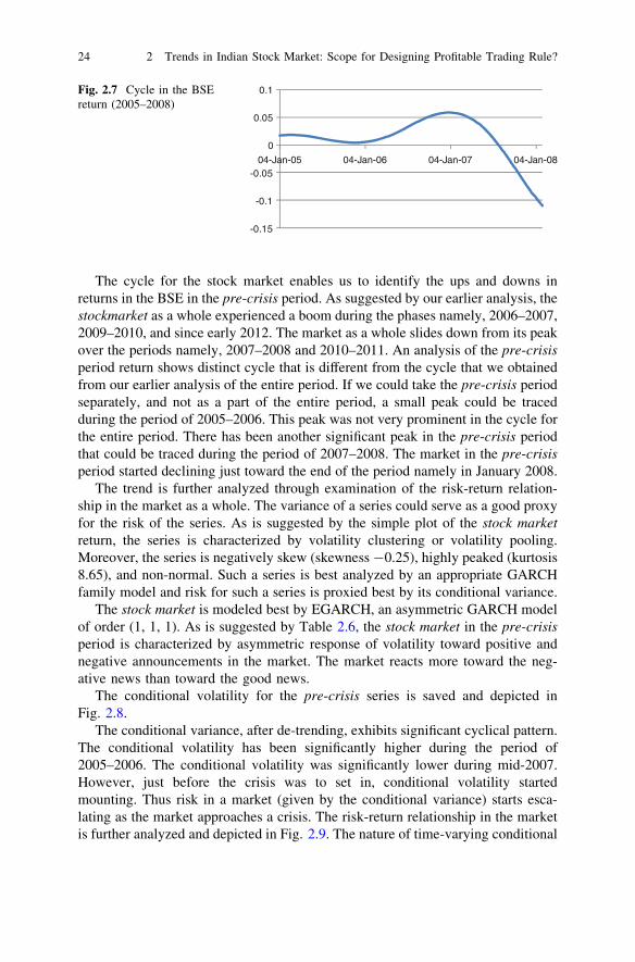
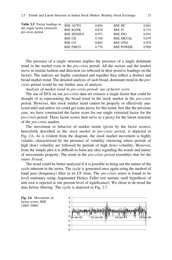
The cycle for the stock market enables us to identify the ups and downs inreturns in the BSE in the pre-crisis period. As suggested by our earlier analysis, thestockmarket as a whole experienced a boom during the phases namely, 2006–2007,2009–2010, and since early 2012. The market as a whole slides down from its peakover the periods namely, 2007–2008 and 2010–2011. An analysis of the pre-crisisperiod return shows distinct cycle that is different from the cycle that we obtainedfrom our earlier analysis of the entire period. If we could take the pre-crisis periodseparately, and not as a part of the entire period, a small peak could be tracedduring the period of 2005–2006. This peak was not very prominent in the cycle forthe entire period. There has been another significant peak in the pre-crisis periodthat could be traced during the period of 2007–2008. The market in the pre-crisisperiod started declining just toward the end of the period namely in January 2008.

The trend is further analyzed through examination of the risk-return relation-ship in the market as a whole. The variance of a series could serve as a good proxyfor the risk of the series. As is suggested by the simple plot of the stock marketreturn, the series is characterized by volatility clustering or volatility pooling.Moreover, the series is negatively skew (skewness -0.25), highly peaked (kurtosis8.65), and non-normal. Such a series is best analyzed by an appropriate GARCHfamily model and risk for such a series is proxied best by its conditional variance.

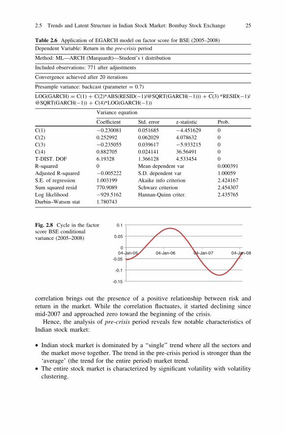
The stock market is modeled best by EGARCH, an asymmetric GARCH modelof order (1, 1, 1). As is suggested by Table 2.6, the stock market in the pre-crisisperiod is characterized by asymmetric response of volatility toward positive andnegative announcements in the market. The market reacts more toward the neg-ative news than toward the good news.

The conditional volatility for the pre-crisis series is saved and depicted inFig. 2.8.

The conditional variance, after de-trending, exhibits significant cyclical pattern.The conditional volatility has been significantly higher during the period of2005–2006. The conditional volatility was significantly lower during mid-2007.However, just before the crisis was to set in, conditional volatility startedmounting. Thus risk in a market (given by the conditional variance) starts esca-lating as the market approaches a crisis. The risk-return relationship in the marketis further analyzed and depicted in Fig. 2.9. The nature of time-varying conditional

-0.15

-0.1

-0.05

0

0.05

0.1

04-Jan-05 04-Jan-06 04-Jan-07 04-Jan-08

Fig. 2.7 Cycle in the BSEreturn (2005–2008)


correlation brings out the presence of a positive relationship between risk andreturn in the market. While the correlation fluctuates, it started declining sincemid-2007 and approached zero toward the beginning of the crisis.

Hence, the analysis of pre-crisis period reveals few notable characteristics ofIndian stock market:

• Indian stock market is dominated by a ‘‘single’’ trend where all the sectors andthe market move together. The trend in the pre-crisis period is stronger than the‘average’ (the trend for the entire period) market trend.

• The entire stock market is characterized by significant volatility with volatilityclustering.


Dependent Variable: Return in the pre-crisis period

Method: ML—ARCH (Marquardt)—Student’s t distribution

Included observations: 771 after adjustments




Variance equation

Coefficient Std. error z-statistic Prob.

C(1) -0.230081 0.051685 -4.451629 0C(2) 0.252992 0.062029 4.078632 0C(3) -0.235055 0.039617 -5.933215 0C(4) 0.882705 0.024141 36.56491 0T-DIST. DOF 6.19328 1.366128 4.533454 0R-squared 0 Mean dependent var 0.000391Adjusted R-squared -0.005222 S.D. dependent var 1.00059S.E. of regression 1.003199 Akaike info criterion 2.424167Sum squared resid 770.9089 Schwarz criterion 2.454307Log likelihood -929.5162 Hannan-Quinn criter. 2.435765Durbin–Watson stat 1.780743

-0.15

-0.1

-0.05

0

0.05

0.1

04-Jan-05 04-Jan-06 04-Jan-07 04-Jan-08



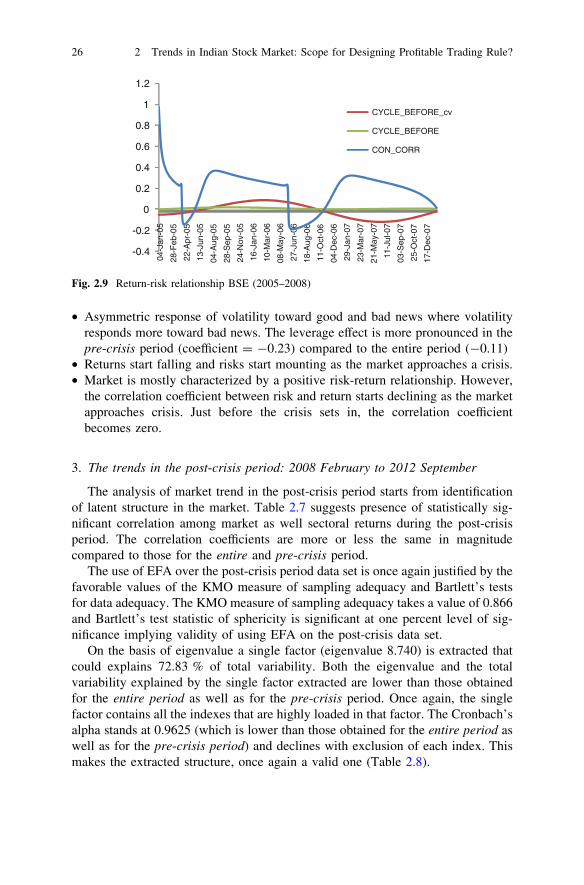
• Asymmetric response of volatility toward good and bad news where volatilityresponds more toward bad news. The leverage effect is more pronounced in thepre-crisis period (coefficient = -0.23) compared to the entire period (-0.11)

• Returns start falling and risks start mounting as the market approaches a crisis.• Market is mostly characterized by a positive risk-return relationship. However,

the correlation coefficient between risk and return starts declining as the marketapproaches crisis. Just before the crisis sets in, the correlation coefficientbecomes zero.

3. The trends in the post-crisis period: 2008 February to 2012 September

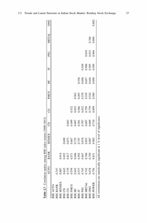
The analysis of market trend in the post-crisis period starts from identificationof latent structure in the market. Table 2.7 suggests presence of statistically sig-nificant correlation among market as well sectoral returns during the post-crisisperiod. The correlation coefficients are more or less the same in magnitudecompared to those for the entire and pre-crisis period.

The use of EFA over the post-crisis period data set is once again justified by thefavorable values of the KMO measure of sampling adequacy and Bartlett’s testsfor data adequacy. The KMO measure of sampling adequacy takes a value of 0.866and Bartlett’s test statistic of sphericity is significant at one percent level of sig-nificance implying validity of using EFA on the post-crisis data set.

On the basis of eigenvalue a single factor (eigenvalue 8.740) is extracted thatcould explains 72.83 % of total variability. Both the eigenvalue and the totalvariability explained by the single factor extracted are lower than those obtainedfor the entire period as well as for the pre-crisis period. Once again, the singlefactor contains all the indexes that are highly loaded in that factor. The Cronbach’salpha stands at 0.9625 (which is lower than those obtained for the entire period aswell as for the pre-crisis period) and declines with exclusion of each index. Thismakes the extracted structure, once again a valid one (Table 2.8).

-0.4

-0.2

0

0.2

0.4

0.6

0.8

1

1.2

04-J

an-0

5

28-F

eb-0

5

22-A

pr-0

5

13-J

un-0

5

04-A

ug-0

5

28-S

ep-0

5

24-N

ov-0

5

16-J

an-0

6

10-M

ar-0

6

08-M

ay-0

6

27-J

un-0

6

18-A

ug-0

6

11-O

ct-0

6

04-D

ec-0

6

29-J

an-0

7

23-M

ar-0

7

21-M

ay-0

7

11-J

ul-0

7

03-S

ep-0

7

25-O

ct-0

7

17-D

ec-0

7

CYCLE_BEFORE_cv

CYCLE_BEFORE

CON_CORR



Tab

le2.

7C

orre

lati

onm

atri

xam

ong

BS

Ein

dex

retu

rns

(200

8–20

12)

AU

TO

BA

NK

SE

NS

EX

CD

CG

FM

CG

HC

ITP

SU

ME

TA

LO

NG

BS

EA

UT

OB

SE

BA

NK

0.74

7B

SE

SE

NS

EX

0.80

70.

914

BS

EC

D0.

642

0.65

20.

698

BS

EC

G0.

739

0.81

70.

873

0.68

3B

SE

FM

CG

0.55

90.

571

0.66

70.

499

0.53

2B

SE

HC

0.64

30.

646

0.72

50.

607

0.65

20.

563

BS

EIT

0.53

70.

592

0.74

70.

501

0.56

60.

493

0.53

6B

SE

PS

U0.

745

0.84

70.

878

0.70

70.

832

0.57

80.

698

0.54

9B

SE

ME

TA

L0.

742

0.76

00.

853

0.68

70.

759

0.53

90.

657

0.58

80.

810

BS

EO

NG

0.67

80.

750

0.88

70.

609

0.73

90.

524

0.64

40.

585

0.81

50.

768

BS

EP

OW

ER

0.75

60.

831

0.90

20.

710

0.89

90.

589

0.69

80.

589

0.90

40.

809

0.80

2

All

corr

elat

ions

are

stat

isti

call

ysi

gnifi

cant

at1

%le

vel

ofsi

gnifi

canc

e


The presence of a single structure implies the presence of a single dominanttrend in the market even in the post-crisis period. All the sectors and the marketmove in similar fashion and direction (as reflected in their positive loadings on thefactor). The indexes are highly correlated and together they reflect a distinct andbroad market trend. The detailed analysis of such broad, dominant trend in thepost-crisis period would be our further area of analysis.

Analysis of market trend in post-crisis period: use of factor scoreThe use of EFA on our post-crisis data set extracts a single factor that could be

thought of as representing the broad trend in the stock market in the post-crisisperiod. However, to analyze this stock market trend properly and effectively, weneed to get some proxy for this trend. Just like the previous two cases, we haveconstructed the factor score for our single extracted factor for the post-crisisperiod. These factor scores then serve as a proxy for the latent structure of the post-crisis market.

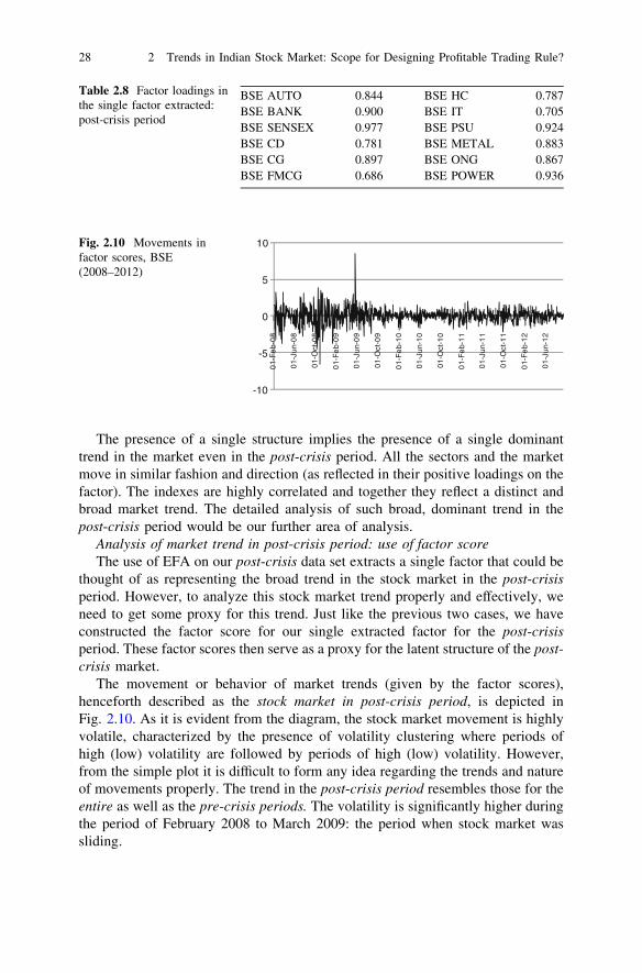
The movement or behavior of market trends (given by the factor scores),henceforth described as the stock market in post-crisis period, is depicted inFig. 2.10. As it is evident from the diagram, the stock market movement is highlyvolatile, characterized by the presence of volatility clustering where periods ofhigh (low) volatility are followed by periods of high (low) volatility. However,from the simple plot it is difficult to form any idea regarding the trends and natureof movements properly. The trend in the post-crisis period resembles those for theentire as well as the pre-crisis periods. The volatility is significantly higher duringthe period of February 2008 to March 2009: the period when stock market wassliding.

Table 2.8 Factor loadings inthe single factor extracted:post-crisis period


-10

-5

0

5

10

01-

Fe

b-0

8

01-

Jun-

08

01-

Oct

-08

01-

Fe

b-0

9

01-

Jun-

09

01-

Oct

-09

01-

Fe

b-1

0

01-

Jun-

10

01-

Oct

-10

01-

Fe

b-1

1

01-

Jun-

11

01-

Oct

-11

01-

Fe

b-1

2

01-

Jun-

12



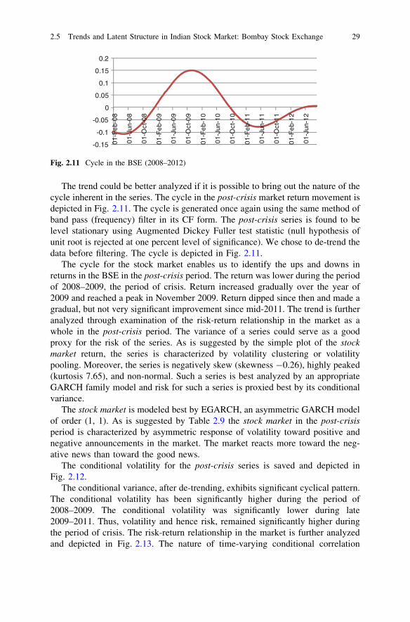
The trend could be better analyzed if it is possible to bring out the nature of thecycle inherent in the series. The cycle in the post-crisis market return movement isdepicted in Fig. 2.11. The cycle is generated once again using the same method ofband pass (frequency) filter in its CF form. The post-crisis series is found to belevel stationary using Augmented Dickey Fuller test statistic (null hypothesis ofunit root is rejected at one percent level of significance). We chose to de-trend thedata before filtering. The cycle is depicted in Fig. 2.11.

The cycle for the stock market enables us to identify the ups and downs inreturns in the BSE in the post-crisis period. The return was lower during the periodof 2008–2009, the period of crisis. Return increased gradually over the year of2009 and reached a peak in November 2009. Return dipped since then and made agradual, but not very significant improvement since mid-2011. The trend is furtheranalyzed through examination of the risk-return relationship in the market as awhole in the post-crisis period. The variance of a series could serve as a goodproxy for the risk of the series. As is suggested by the simple plot of the stockmarket return, the series is characterized by volatility clustering or volatilitypooling. Moreover, the series is negatively skew (skewness -0.26), highly peaked(kurtosis 7.65), and non-normal. Such a series is best analyzed by an appropriateGARCH family model and risk for such a series is proxied best by its conditionalvariance.

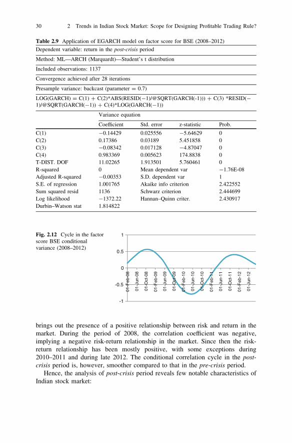
The stock market is modeled best by EGARCH, an asymmetric GARCH modelof order (1, 1). As is suggested by Table 2.9 the stock market in the post-crisisperiod is characterized by asymmetric response of volatility toward positive andnegative announcements in the market. The market reacts more toward the neg-ative news than toward the good news.

The conditional volatility for the post-crisis series is saved and depicted inFig. 2.12.

The conditional variance, after de-trending, exhibits significant cyclical pattern.The conditional volatility has been significantly higher during the period of2008–2009. The conditional volatility was significantly lower during late2009–2011. Thus, volatility and hence risk, remained significantly higher duringthe period of crisis. The risk-return relationship in the market is further analyzedand depicted in Fig. 2.13. The nature of time-varying conditional correlation

-0.15

-0.1

-0.05

0

0.05

0.1

0.15

0.2

01-

Fe

b-0

8

01-

Jun-

08

01-

Oct

-08

01-

Fe

b-0

9

01-

Jun-

09

01-

Oct

-09

01-

Fe

b-1

0

01-

Jun-

10

01-

Oct

-10

01-

Fe

b-1

1

01-

Jun-

11

01-

Oct

-11

01-

Fe

b-1

2

01-

Jun-

12

Fig. 2.11 Cycle in the BSE (2008–2012)


brings out the presence of a positive relationship between risk and return in themarket. During the period of 2008, the correlation coefficient was negative,implying a negative risk-return relationship in the market. Since then the risk-return relationship has been mostly positive, with some exceptions during2010–2011 and during late 2012. The conditional correlation cycle in the post-crisis period is, however, smoother compared to that in the pre-crisis period.

Hence, the analysis of post-crisis period reveals few notable characteristics ofIndian stock market:


Dependent variable: return in the post-crisis period

Method: ML—ARCH (Marquardt)—Student’s t distribution

Included observations: 1137




Variance equation


C(1) -0.14429 0.025556 -5.64629 0C(2) 0.17386 0.03189 5.451858 0C(3) -0.08342 0.017128 -4.87047 0C(4) 0.983369 0.005623 174.8838 0T-DIST. DOF 11.02265 1.913501 5.760461 0R-squared 0 Mean dependent var -1.76E-08Adjusted R-squared -0.00353 S.D. dependent var 1S.E. of regression 1.001765 Akaike info criterion 2.422552Sum squared resid 1136 Schwarz criterion 2.444699Log likelihood -1372.22 Hannan–Quinn criter. 2.430917Durbin–Watson stat 1.814822

-1

-0.5

0

0.5

1

01-F

eb-0

8

01-J

un-0

8

01-O

ct-0

8

01-F

eb-0

9

01-J

un-0

9

01-O

ct-0

9

01-F

eb-1

0

01-J

un-1

0

01-O

ct-1

0

01-F

eb-1

1

01-J

un-1

1

01-O

ct-1

1

01-F

eb-1

2

01-J

un-1

2



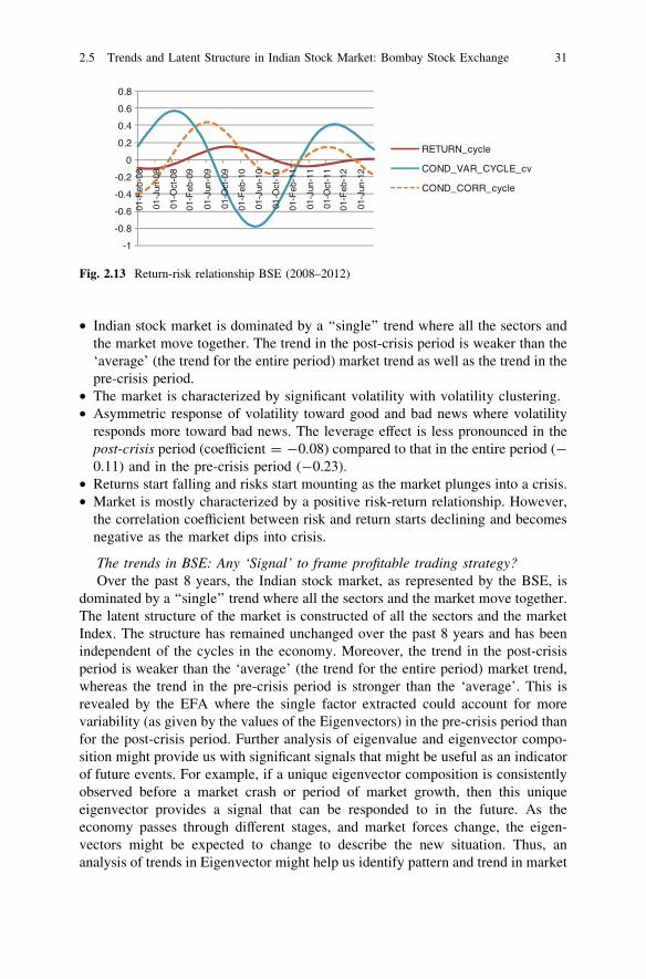
• Indian stock market is dominated by a ‘‘single’’ trend where all the sectors andthe market move together. The trend in the post-crisis period is weaker than the‘average’ (the trend for the entire period) market trend as well as the trend in thepre-crisis period.

• The market is characterized by significant volatility with volatility clustering.• Asymmetric response of volatility toward good and bad news where volatility

responds more toward bad news. The leverage effect is less pronounced in thepost-crisis period (coefficient = -0.08) compared to that in the entire period (-0.11) and in the pre-crisis period (-0.23).

• Returns start falling and risks start mounting as the market plunges into a crisis.• Market is mostly characterized by a positive risk-return relationship. However,

the correlation coefficient between risk and return starts declining and becomesnegative as the market dips into crisis.

The trends in BSE: Any ‘Signal’ to frame profitable trading strategy?Over the past 8 years, the Indian stock market, as represented by the BSE, is

dominated by a ‘‘single’’ trend where all the sectors and the market move together.The latent structure of the market is constructed of all the sectors and the marketIndex. The structure has remained unchanged over the past 8 years and has beenindependent of the cycles in the economy. Moreover, the trend in the post-crisisperiod is weaker than the ‘average’ (the trend for the entire period) market trend,whereas the trend in the pre-crisis period is stronger than the ‘average’. This isrevealed by the EFA where the single factor extracted could account for morevariability (as given by the values of the Eigenvectors) in the pre-crisis period thanfor the post-crisis period. Further analysis of eigenvalue and eigenvector compo-sition might provide us with significant signals that might be useful as an indicatorof future events. For example, if a unique eigenvector composition is consistentlyobserved before a market crash or period of market growth, then this uniqueeigenvector provides a signal that can be responded to in the future. As theeconomy passes through different stages, and market forces change, the eigen-vectors might be expected to change to describe the new situation. Thus, ananalysis of trends in Eigenvector might help us identify pattern and trend in market

-1

-0.8

-0.6

-0.4

-0.2

0

0.2

0.4

0.6

0.8

RETURN_cycle

COND_VAR_CYCLE_cv

COND_CORR_cycle

01-F

eb-0

8

01-J

un-0

8

01-O

ct-0

8

01-F

eb-0

9

01-J

un-0

9

01-O

ct-0

9

01-F

eb-1

0

01-J

un-1

0

01-O

ct-1

0

01-F

eb-1

1

01-J

un-1

1

01-O

ct-1

1

01-F

eb-1

2

01-J

un-1

2



movements. This in turn might help investors design strategies that would reducerisk and increase gains.

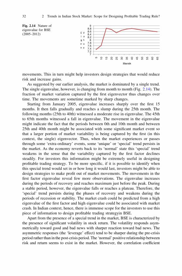
As suggested by our earlier analysis, the market is dominated by a single trend.The single eigenvalue, however, is changing from month to month (Fig. 2.14). Thefraction of market variation captured by the first eigenvector thus changes overtime. The movements are sometime marked by sharp changes.

Starting from January 2005, eigenvalue increases sharply over the first 15months. It then falls gradually and reaches a slump during the 25th month. Thefollowing months (25th to 40th) witnessed a moderate rise in eigenvalue. The 45thto 65th months witnessed a fall in eigenvalue. The movement in the eigenvaluemight indicate the fact that the periods between 0th and 10th month and between25th and 40th month might be associated with some significant market event sothat a larger portion of market variability is being captured by the first (in thiscontext, the single) eigenvector. Thus, when the market experiences or passesthrough some ‘extra-ordinary’ events, some ‘unique’ or ‘special’ trend persists inthe market. As the economy reverts back to its ‘normal’ state this ‘special’ trendweakens in the sense that the variability captured by the first factor declinessteadily. For investors this information might be extremely useful in designingprofitable trading strategy. To be more specific, if it is possible to identify whenthis special trend would set in or how long it would last, investors might be able todesign strategies to make profit out of market movements. The movements in thefirst factor eigenvalue reveal few more observations. The eigenvalue increasesduring the periods of recovery and reaches maximum just before the peak. Duringa stable period, however, the eigenvalue falls or reaches a plateau. Therefore, the‘special’ trend persists during the phases of recovery and weakens during theperiods of recession or stability. The market crash could be predicted from a higheigenvalue of the first factor and high eigenvalue could be associated with marketcrash. In Indian context, hence, there is immense scope for the investors to use thispiece of information to design profitable trading strategyin BSE.

Apart from the presence of a special trend in the market, BSE is characterized bythe presence of significant volatility in stock return. The volatility responds asym-metrically toward good and bad news with sharper reaction toward bad news. Theasymmetric responses (the ‘leverage’ effect) tend to be sharper during the pre-crisisperiod rather than in the post-crisis period. The ‘normal’ positive relationship betweenrisk and return seems to exist in the market. However, the correlation coefficient

77.27.47.67.8

88.28.48.68.8

9

5 10

15

20

25

30

35

40

45

50

55

60

65

Eige

n

Valu

e

Month

Fig. 2.14 Nature ofeigenvalue for BSE(2005–2012)


between risk and return starts declining and becomes negative (or even zero) as themarket dips into crisis. Distinct and persistent trends thus are perceptible in the Indianstock market leaving the efficient market hypothesis on trial. Such trends couldskillfully be used by investors to design profit making strategies to beat the market.

Let us now consider the other stock exchange, namely the NSE and explorewhether the movements and other characteristics in the NSE resemble the trends inBSE. While exploring the issues, we shall be following the same methodologiesthat were followed in the previous sections. Hence, we are not repeating themethodology, but reporting the results only focusing on the analytical discussion.

2.6 Trends and Latent Structure in Indian Stock Market:National Stock Exchange

1. Trends over the entire period: 2005 January to 2012 September

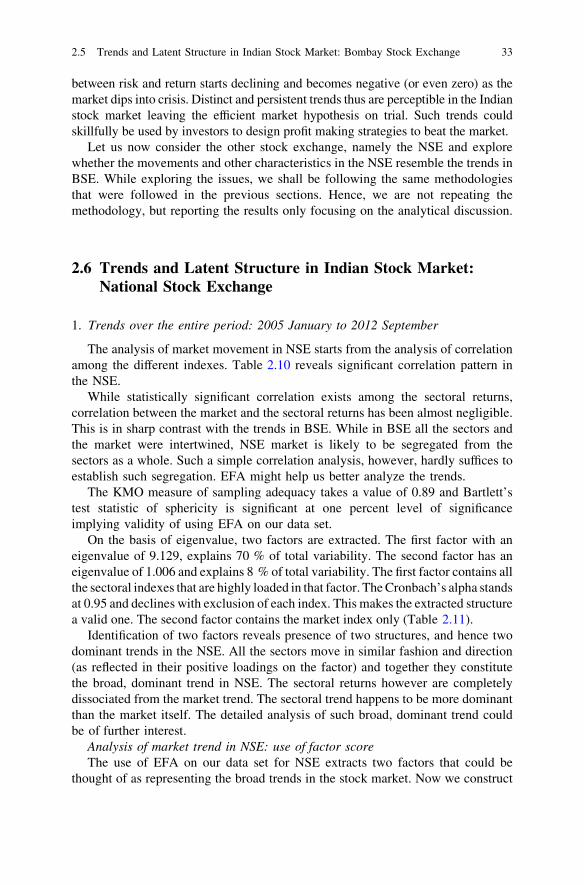
The analysis of market movement in NSE starts from the analysis of correlationamong the different indexes. Table 2.10 reveals significant correlation pattern inthe NSE.

While statistically significant correlation exists among the sectoral returns,correlation between the market and the sectoral returns has been almost negligible.This is in sharp contrast with the trends in BSE. While in BSE all the sectors andthe market were intertwined, NSE market is likely to be segregated from thesectors as a whole. Such a simple correlation analysis, however, hardly suffices toestablish such segregation. EFA might help us better analyze the trends.

The KMO measure of sampling adequacy takes a value of 0.89 and Bartlett’stest statistic of sphericity is significant at one percent level of significanceimplying validity of using EFA on our data set.

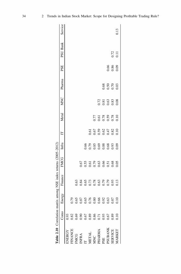
On the basis of eigenvalue, two factors are extracted. The first factor with aneigenvalue of 9.129, explains 70 % of total variability. The second factor has aneigenvalue of 1.006 and explains 8 % of total variability. The first factor contains allthe sectoral indexes that are highly loaded in that factor. The Cronbach’s alpha standsat 0.95 and declines with exclusion of each index. This makes the extracted structurea valid one. The second factor contains the market index only (Table 2.11).

Identification of two factors reveals presence of two structures, and hence twodominant trends in the NSE. All the sectors move in similar fashion and direction(as reflected in their positive loadings on the factor) and together they constitutethe broad, dominant trend in NSE. The sectoral returns however are completelydissociated from the market trend. The sectoral trend happens to be more dominantthan the market itself. The detailed analysis of such broad, dominant trend couldbe of further interest.

Analysis of market trend in NSE: use of factor scoreThe use of EFA on our data set for NSE extracts two factors that could be

thought of as representing the broad trends in the stock market. Now we construct


Tab

le2.

10C

orre

lati

onm

atri

xam

ong

NS

Ein

dex

retu

rns

(200

5–20

12)

Com

oE

nerg

yF

inan

ceF

MC

GIn

fra

ITM

etal

MN

CP

harm

aP

SE

PS

UB

ank

Ser

vice

EN

ER

GY

0.93

FIN

AN

CE

0.82

0.79

FM

CG

0.69

0.65

0.63

INF

RA

0.90

0.87

0.84

0.67

IT0.

670.

650.

650.

550.

66M

ET

AL

0.89

0.76

0.73

0.61

0.79

0.61

MN

C0.

860.

800.

780.

790.

850.

670.

77P

HA

RM

A0.

710.

660.

630.

630.

690.

590.

610.

72P

SE

0.93

0.92

0.79

0.66

0.88

0.62

0.78

0.81

0.68

PS

UB

AN

K0.

670.

630.

790.

510.

680.

470.

590.

630.

500.

66S

ER

VIC

E0.

890.

870.

930.

680.

930.

820.

780.

830.

700.

860.

72M

AR

KE

T0.

100.

100.

130.

050.

090.

100.

100.

080.

030.

090.

110.

13


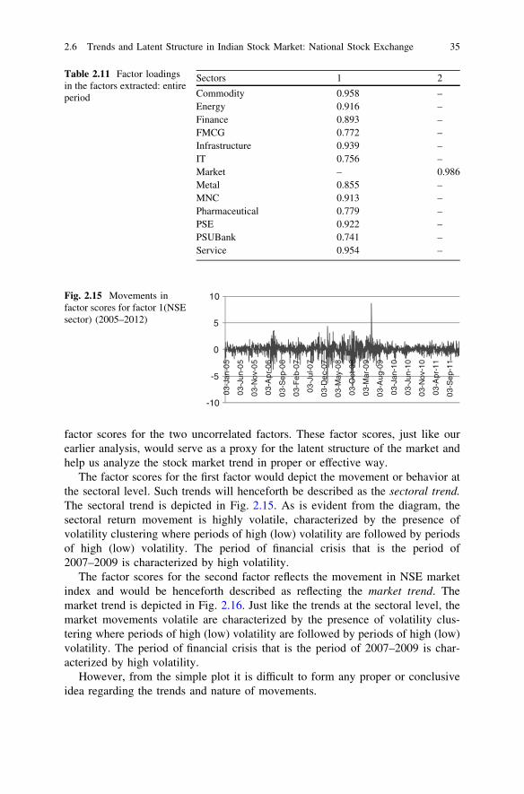
factor scores for the two uncorrelated factors. These factor scores, just like ourearlier analysis, would serve as a proxy for the latent structure of the market andhelp us analyze the stock market trend in proper or effective way.

The factor scores for the first factor would depict the movement or behavior atthe sectoral level. Such trends will henceforth be described as the sectoral trend.The sectoral trend is depicted in Fig. 2.15. As is evident from the diagram, thesectoral return movement is highly volatile, characterized by the presence ofvolatility clustering where periods of high (low) volatility are followed by periodsof high (low) volatility. The period of financial crisis that is the period of2007–2009 is characterized by high volatility.

The factor scores for the second factor reflects the movement in NSE marketindex and would be henceforth described as reflecting the market trend. Themarket trend is depicted in Fig. 2.16. Just like the trends at the sectoral level, themarket movements volatile are characterized by the presence of volatility clus-tering where periods of high (low) volatility are followed by periods of high (low)volatility. The period of financial crisis that is the period of 2007–2009 is char-acterized by high volatility.

However, from the simple plot it is difficult to form any proper or conclusiveidea regarding the trends and nature of movements.

Table 2.11 Factor loadingsin the factors extracted: entireperiod

Sectors 1 2

Commodity 0.958 –Energy 0.916 –Finance 0.893 –FMCG 0.772 –Infrastructure 0.939 –IT 0.756 –Market – 0.986Metal 0.855 –MNC 0.913 –Pharmaceutical 0.779 –PSE 0.922 –PSUBank 0.741 –Service 0.954 –

-10

-5

0

5

10

03-

Jan-

05

03-

Jun-

05

03-

Nov

-05

03-

Apr

-06

03-

Se

p-0

6

03-

Fe

b-0

7

03-

Jul-0

7

03-

De

c-0

7

03-

May

-08

03-

Oct

-08

03-

Mar

-09

03-

Aug

-09

03-

Jan-

10

03-

Jun-

10

03-

Nov

-10

03-

Apr

-11

03-

Se

p-1

1

Fig. 2.15 Movements infactor scores for factor 1(NSEsector) (2005–2012)

2.6 Trends and Latent Structure in Indian Stock Market: National Stock Exchange 35

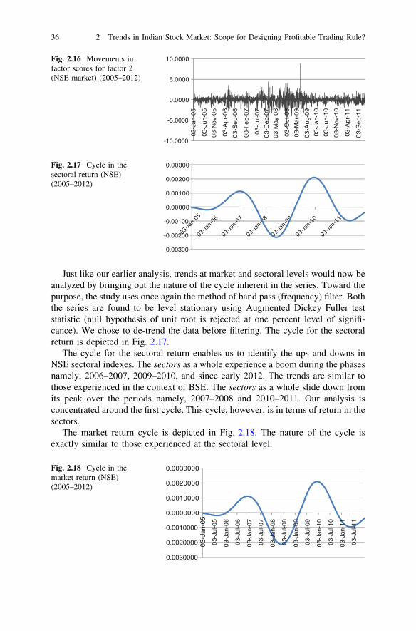
Just like our earlier analysis, trends at market and sectoral levels would now beanalyzed by bringing out the nature of the cycle inherent in the series. Toward thepurpose, the study uses once again the method of band pass (frequency) filter. Boththe series are found to be level stationary using Augmented Dickey Fuller teststatistic (null hypothesis of unit root is rejected at one percent level of signifi-cance). We chose to de-trend the data before filtering. The cycle for the sectoralreturn is depicted in Fig. 2.17.

The cycle for the sectoral return enables us to identify the ups and downs inNSE sectoral indexes. The sectors as a whole experience a boom during the phasesnamely, 2006–2007, 2009–2010, and since early 2012. The trends are similar tothose experienced in the context of BSE. The sectors as a whole slide down fromits peak over the periods namely, 2007–2008 and 2010–2011. Our analysis isconcentrated around the first cycle. This cycle, however, is in terms of return in thesectors.

The market return cycle is depicted in Fig. 2.18. The nature of the cycle isexactly similar to those experienced at the sectoral level.

-10.0000

-5.0000

0.0000

5.0000

10.0000

03-

Jan-

05

03-

Jun-

05

03-

Nov

-05

03-

Apr

-06

03-

Se

p-0

6

03-

Fe

b-0

7

03-

Jul-0

7

03-

De

c-0

7

03-

May

-08

03-

Oct

-08

03-

Mar

-09

03-

Aug

-09

03-

Jan-

10

03-

Jun-

10

03-

Nov

-10

03-

Apr

-11

03-

Se

p-1

1

Fig. 2.16 Movements infactor scores for factor 2(NSE market) (2005–2012)

-0.00300

-0.00200

-0.00100

0.00000

0.00100

0.00200

0.00300Fig. 2.17 Cycle in thesectoral return (NSE)(2005–2012)

-0.0030000

-0.0020000

-0.0010000

0.0000000

0.0010000

0.0020000

0.0030000

03-

Jan-

05

03-

Jul-0

5

03-

Jan-

06

03-

Jul-0

6

03-

Jan-

07

03-

Jul-0

7

03-

Jan-

08

03-

Jul-0

8

03-

Jan-

09

03-

Jul-0

9

03-

Jan-

10

03-

Jul-1

0

03-

Jan-

11

03-

Jul-1

1

Fig. 2.18 Cycle in themarket return (NSE)(2005–2012)


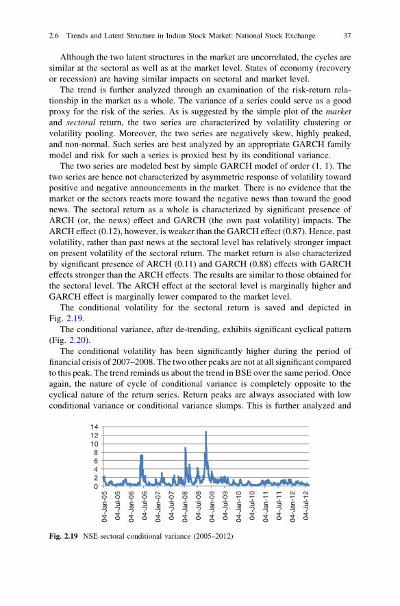
Although the two latent structures in the market are uncorrelated, the cycles aresimilar at the sectoral as well as at the market level. States of economy (recoveryor recession) are having similar impacts on sectoral and market level.

The trend is further analyzed through an examination of the risk-return rela-tionship in the market as a whole. The variance of a series could serve as a goodproxy for the risk of the series. As is suggested by the simple plot of the marketand sectoral return, the two series are characterized by volatility clustering orvolatility pooling. Moreover, the two series are negatively skew, highly peaked,and non-normal. Such series are best analyzed by an appropriate GARCH familymodel and risk for such a series is proxied best by its conditional variance.

The two series are modeled best by simple GARCH model of order (1, 1). Thetwo series are hence not characterized by asymmetric response of volatility towardpositive and negative announcements in the market. There is no evidence that themarket or the sectors reacts more toward the negative news than toward the goodnews. The sectoral return as a whole is characterized by significant presence ofARCH (or, the news) effect and GARCH (the own past volatility) impacts. TheARCH effect (0.12), however, is weaker than the GARCH effect (0.87). Hence, pastvolatility, rather than past news at the sectoral level has relatively stronger impacton present volatility of the sectoral return. The market return is also characterizedby significant presence of ARCH (0.11) and GARCH (0.88) effects with GARCHeffects stronger than the ARCH effects. The results are similar to those obtained forthe sectoral level. The ARCH effect at the sectoral level is marginally higher andGARCH effect is marginally lower compared to the market level.

The conditional volatility for the sectoral return is saved and depicted inFig. 2.19.

The conditional variance, after de-trending, exhibits significant cyclical pattern(Fig. 2.20).

The conditional volatility has been significantly higher during the period offinancial crisis of 2007–2008. The two other peaks are not at all significant comparedto this peak. The trend reminds us about the trend in BSE over the same period. Onceagain, the nature of cycle of conditional variance is completely opposite to thecyclical nature of the return series. Return peaks are always associated with lowconditional variance or conditional variance slumps. This is further analyzed and

02468

101214

04-

Jan-

05

04-

Jul-0

5

04-

Jan-

06

04-

Jul-0

6

04-

Jan-

07

04-

Jul-0

7

04-

Jan-

08

04-

Jul-0

8

04-

Jan-

09

04-

Jul-0

9

04-

Jan-

10

04-

Jul-1

0

04-

Jan-

11

04-

Jul-1

1

04-

Jan-

12

04-

Jul-1

2

Fig. 2.19 NSE sectoral conditional variance (2005–2012)


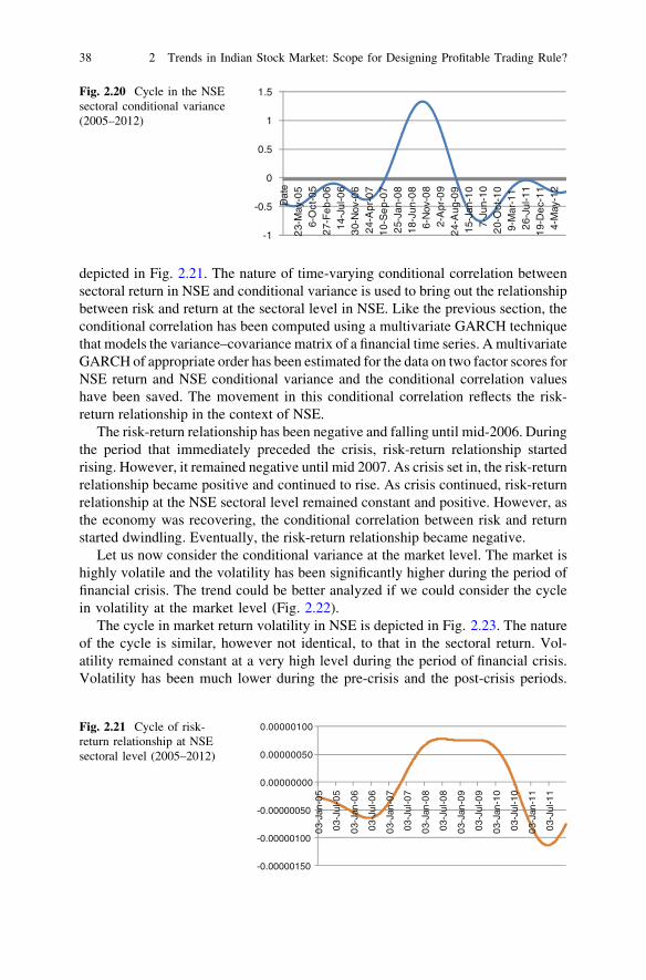
depicted in Fig. 2.21. The nature of time-varying conditional correlation betweensectoral return in NSE and conditional variance is used to bring out the relationshipbetween risk and return at the sectoral level in NSE. Like the previous section, theconditional correlation has been computed using a multivariate GARCH techniquethat models the variance–covariance matrix of a financial time series. A multivariateGARCH of appropriate order has been estimated for the data on two factor scores forNSE return and NSE conditional variance and the conditional correlation valueshave been saved. The movement in this conditional correlation reflects the risk-return relationship in the context of NSE.

The risk-return relationship has been negative and falling until mid-2006. Duringthe period that immediately preceded the crisis, risk-return relationship startedrising. However, it remained negative until mid 2007. As crisis set in, the risk-returnrelationship became positive and continued to rise. As crisis continued, risk-returnrelationship at the NSE sectoral level remained constant and positive. However, asthe economy was recovering, the conditional correlation between risk and returnstarted dwindling. Eventually, the risk-return relationship became negative.

Let us now consider the conditional variance at the market level. The market ishighly volatile and the volatility has been significantly higher during the period offinancial crisis. The trend could be better analyzed if we could consider the cyclein volatility at the market level (Fig. 2.22).

The cycle in market return volatility in NSE is depicted in Fig. 2.23. The natureof the cycle is similar, however not identical, to that in the sectoral return. Vol-atility remained constant at a very high level during the period of financial crisis.Volatility has been much lower during the pre-crisis and the post-crisis periods.

-1

-0.5

0

0.5

1

1.5

Dat

e2

3-M

ay-0

56-

Oct

-05

27-

Fe

b-0

61

4-Ju

l-06

30-

Nov

-06

24-

Apr

-07

10-

Se

p-0

72

5-Ja

n-0

81

8-Ju

n-0

86-

Nov

-08

2-A

pr-0

92

4-A

ug-0

91

5-Ja

n-1

07-

Jun-

10

20-

Oct

-10

9-M

ar-1

1 2

6-Ju

l-11

19-

De

c-1

14-

May

-12

Fig. 2.20 Cycle in the NSEsectoral conditional variance(2005–2012)

-0.00000150

-0.00000100

-0.00000050

0.00000000

0.00000050

0.00000100

03-

Jan-

05

03-

Jul-0

5

03-

Jan-

06

03-

Jul-0

6

03-

Jan-

07

03-

Jul-0

7

03-

Jan-

08

03-

Jul-0

8

03-

Jan-

09

03-

Jul-0

9

03-

Jan-

10

03-

Jul-1

0

03-

Jan-

11

03-

Jul-1

1

Fig. 2.21 Cycle of risk-return relationship at NSEsectoral level (2005–2012)


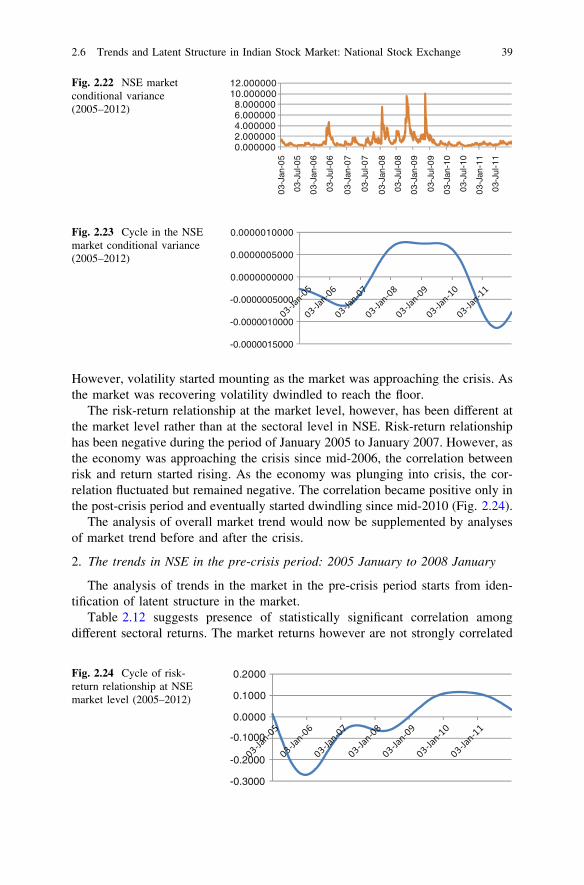
However, volatility started mounting as the market was approaching the crisis. Asthe market was recovering volatility dwindled to reach the floor.

The risk-return relationship at the market level, however, has been different atthe market level rather than at the sectoral level in NSE. Risk-return relationshiphas been negative during the period of January 2005 to January 2007. However, asthe economy was approaching the crisis since mid-2006, the correlation betweenrisk and return started rising. As the economy was plunging into crisis, the cor-relation fluctuated but remained negative. The correlation became positive only inthe post-crisis period and eventually started dwindling since mid-2010 (Fig. 2.24).

The analysis of overall market trend would now be supplemented by analysesof market trend before and after the crisis.

2. The trends in NSE in the pre-crisis period: 2005 January to 2008 January

The analysis of trends in the market in the pre-crisis period starts from iden-tification of latent structure in the market.

Table 2.12 suggests presence of statistically significant correlation amongdifferent sectoral returns. The market returns however are not strongly correlated

0.0000002.0000004.0000006.0000008.000000

10.00000012.000000

03-

Jan-

05

03-

Jul-0

5

03-

Jan-

06

03-

Jul-0

6

03-

Jan-

07

03-

Jul-0

7

03-

Jan-

08

03-

Jul-0

8

03-

Jan-

09

03-

Jul-0

9

03-

Jan-

10

03-

Jul-1

0

03-

Jan-

11

03-

Jul-1

1

Fig. 2.22 NSE marketconditional variance(2005–2012)

-0.0000015000

-0.0000010000

-0.0000005000

0.0000000000

0.0000005000

0.0000010000Fig. 2.23 Cycle in the NSEmarket conditional variance(2005–2012)

-0.3000

-0.2000

-0.1000

0.0000

0.1000

0.2000Fig. 2.24 Cycle of risk-return relationship at NSEmarket level (2005–2012)


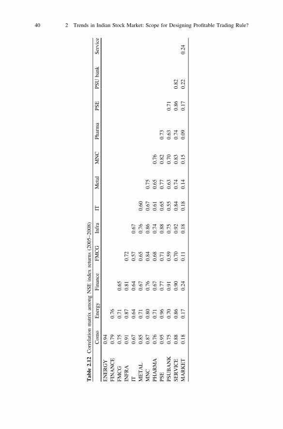
Tab

le2.

12C

orre

lati

onm

atri

xam

ong

NS

Ein

dex

retu

rns

(200

5–20

08)

Com

oE

nerg

yF

inan

ceF

MC

GIn

fra

ITM

etal

MN

CP

harm

aP

SE

PS

Uba

nkS

ervi

ce

EN

ER

GY

0.94

FIN

AN

CE

0.79

0.76

FM

CG

0.75

0.71

0.65

INF

RA

0.91

0.87

0.81

0.72

IT0.

670.

640.

640.

570.

67M

ET

AL

0.85

0.71

0.67

0.65

0.76

0.60

MN

C0.

870.

800.

760.

840.

860.

670.

75P

HA

RM

A0.

760.

710.

670.

680.

740.

610.

650.

76P

SE

0.95

0.96

0.77

0.71

0.88

0.65

0.77

0.82

0.73

PS

UB

AN

K0.

750.

700.

910.

590.

750.

550.

630.

700.

630.

71S

ER

VIC

E0.

880.

860.

900.

700.

920.

840.

740.

830.

740.

860.

82M

AR

KE

T0.

180.

170.

240.

110.

180.

180.

140.

150.

090.

170.

220.

24


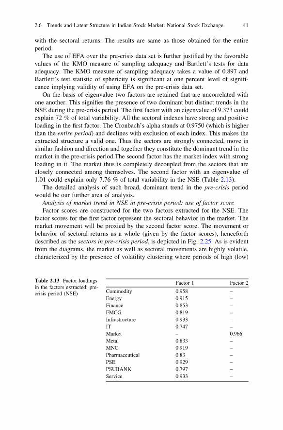
with the sectoral returns. The results are same as those obtained for the entireperiod.

The use of EFA over the pre-crisis data set is further justified by the favorablevalues of the KMO measure of sampling adequacy and Bartlett’s tests for dataadequacy. The KMO measure of sampling adequacy takes a value of 0.897 andBartlett’s test statistic of sphericity is significant at one percent level of signifi-cance implying validity of using EFA on the pre-crisis data set.

On the basis of eigenvalue two factors are retained that are uncorrelated withone another. This signifies the presence of two dominant but distinct trends in theNSE during the pre-crisis period. The first factor with an eigenvalue of 9.373 couldexplain 72 % of total variability. All the sectoral indexes have strong and positiveloading in the first factor. The Cronbach’s alpha stands at 0.9750 (which is higherthan the entire period) and declines with exclusion of each index. This makes theextracted structure a valid one. Thus the sectors are strongly connected, move insimilar fashion and direction and together they constitute the dominant trend in themarket in the pre-crisis period.The second factor has the market index with strongloading in it. The market thus is completely decoupled from the sectors that areclosely connected among themselves. The second factor with an eigenvalue of1.01 could explain only 7.76 % of total variability in the NSE (Table 2.13).

The detailed analysis of such broad, dominant trend in the pre-crisis periodwould be our further area of analysis.

Analysis of market trend in NSE in pre-crisis period: use of factor scoreFactor scores are constructed for the two factors extracted for the NSE. The

factor scores for the first factor represent the sectoral behavior in the market. Themarket movement will be proxied by the second factor score. The movement orbehavior of sectoral returns as a whole (given by the factor scores), henceforthdescribed as the sectors in pre-crisis period, is depicted in Fig. 2.25. As is evidentfrom the diagrams, the market as well as sectoral movements are highly volatile,characterized by the presence of volatility clustering where periods of high (low)

Table 2.13 Factor loadingsin the factors extracted: pre-crisis period (NSE)

Factor 1 Factor 2

Commodity 0.958 –Energy 0.915 –Finance 0.853 –FMCG 0.819 –Infrastructure 0.933 –IT 0.747 –Market – 0.966Metal 0.833 –MNC 0.919 –Pharmaceutical 0.83 –PSE 0.929 –PSUBANK 0.797 –Service 0.933 –


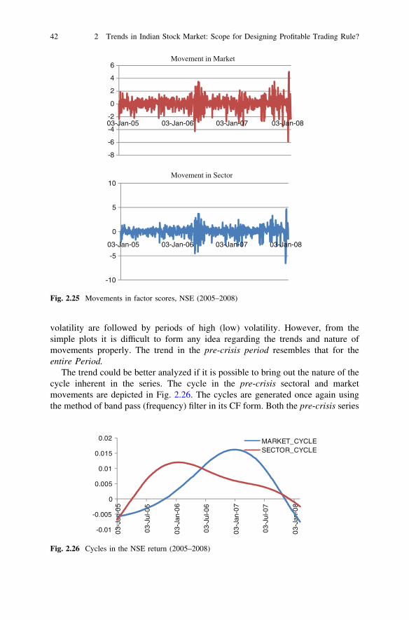
volatility are followed by periods of high (low) volatility. However, from thesimple plots it is difficult to form any idea regarding the trends and nature ofmovements properly. The trend in the pre-crisis period resembles that for theentire Period.

The trend could be better analyzed if it is possible to bring out the nature of thecycle inherent in the series. The cycle in the pre-crisis sectoral and marketmovements are depicted in Fig. 2.26. The cycles are generated once again usingthe method of band pass (frequency) filter in its CF form. Both the pre-crisis series

-8

-6

-4

-2

0

2

4

6

03-Jan-05 03-Jan-06 03-Jan-07 03-Jan-08

Movement in Market

-10

-5

0

5

10

03-Jan-05 03-Jan-06 03-Jan-07 03-Jan-08

Movement in Sector

Fig. 2.25 Movements in factor scores, NSE (2005–2008)

-0.01

-0.005

0

0.005

0.01

0.015

0.02

03-

Jan-

05

03-

Jul-0

5

03-

Jan-

06

03-

Jul-0

6

03-

Jan-

07

03-

Jul-0

7

03-

Jan-

08

MARKET_CYCLESECTOR_CYCLE

Fig. 2.26 Cycles in the NSE return (2005–2008)


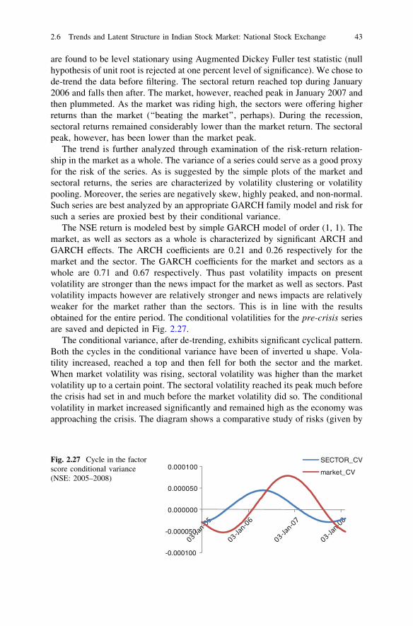
are found to be level stationary using Augmented Dickey Fuller test statistic (nullhypothesis of unit root is rejected at one percent level of significance). We chose tode-trend the data before filtering. The sectoral return reached top during January2006 and falls then after. The market, however, reached peak in January 2007 andthen plummeted. As the market was riding high, the sectors were offering higherreturns than the market (‘‘beating the market’’, perhaps). During the recession,sectoral returns remained considerably lower than the market return. The sectoralpeak, however, has been lower than the market peak.

The trend is further analyzed through examination of the risk-return relation-ship in the market as a whole. The variance of a series could serve as a good proxyfor the risk of the series. As is suggested by the simple plots of the market andsectoral returns, the series are characterized by volatility clustering or volatilitypooling. Moreover, the series are negatively skew, highly peaked, and non-normal.Such series are best analyzed by an appropriate GARCH family model and risk forsuch a series are proxied best by their conditional variance.

The NSE return is modeled best by simple GARCH model of order (1, 1). Themarket, as well as sectors as a whole is characterized by significant ARCH andGARCH effects. The ARCH coefficients are 0.21 and 0.26 respectively for themarket and the sector. The GARCH coefficients for the market and sectors as awhole are 0.71 and 0.67 respectively. Thus past volatility impacts on presentvolatility are stronger than the news impact for the market as well as sectors. Pastvolatility impacts however are relatively stronger and news impacts are relativelyweaker for the market rather than the sectors. This is in line with the resultsobtained for the entire period. The conditional volatilities for the pre-crisis seriesare saved and depicted in Fig. 2.27.

The conditional variance, after de-trending, exhibits significant cyclical pattern.Both the cycles in the conditional variance have been of inverted u shape. Vola-tility increased, reached a top and then fell for both the sector and the market.When market volatility was rising, sectoral volatility was higher than the marketvolatility up to a certain point. The sectoral volatility reached its peak much beforethe crisis had set in and much before the market volatility did so. The conditionalvolatility in market increased significantly and remained high as the economy wasapproaching the crisis. The diagram shows a comparative study of risks (given by

-0.000100

-0.000050

0.000000

0.000050

0.000100SECTOR_CV

market_CV

Fig. 2.27 Cycle in the factorscore conditional variance(NSE: 2005–2008)


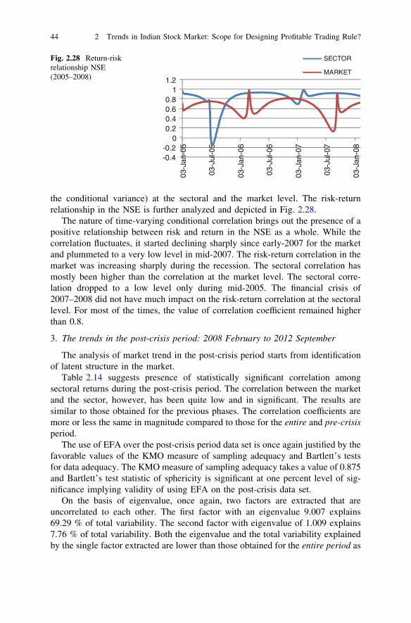
the conditional variance) at the sectoral and the market level. The risk-returnrelationship in the NSE is further analyzed and depicted in Fig. 2.28.

The nature of time-varying conditional correlation brings out the presence of apositive relationship between risk and return in the NSE as a whole. While thecorrelation fluctuates, it started declining sharply since early-2007 for the marketand plummeted to a very low level in mid-2007. The risk-return correlation in themarket was increasing sharply during the recession. The sectoral correlation hasmostly been higher than the correlation at the market level. The sectoral corre-lation dropped to a low level only during mid-2005. The financial crisis of2007–2008 did not have much impact on the risk-return correlation at the sectorallevel. For most of the times, the value of correlation coefficient remained higherthan 0.8.

3. The trends in the post-crisis period: 2008 February to 2012 September

The analysis of market trend in the post-crisis period starts from identificationof latent structure in the market.

Table 2.14 suggests presence of statistically significant correlation amongsectoral returns during the post-crisis period. The correlation between the marketand the sector, however, has been quite low and in significant. The results aresimilar to those obtained for the previous phases. The correlation coefficients aremore or less the same in magnitude compared to those for the entire and pre-crisisperiod.

The use of EFA over the post-crisis period data set is once again justified by thefavorable values of the KMO measure of sampling adequacy and Bartlett’s testsfor data adequacy. The KMO measure of sampling adequacy takes a value of 0.875and Bartlett’s test statistic of sphericity is significant at one percent level of sig-nificance implying validity of using EFA on the post-crisis data set.

On the basis of eigenvalue, once again, two factors are extracted that areuncorrelated to each other. The first factor with an eigenvalue 9.007 explains69.29 % of total variability. The second factor with eigenvalue of 1.009 explains7.76 % of total variability. Both the eigenvalue and the total variability explainedby the single factor extracted are lower than those obtained for the entire period as

-0.4-0.2

00.20.40.60.8

11.2

03-J

an-0

5

03-J

ul-0

5

03-J

an-0

6

03-J

ul-0

6

03-J

an-0

7

03-J

ul-0

7

03-J

an-0

8

SECTOR

MARKET

Fig. 2.28 Return-riskrelationship NSE(2005–2008)


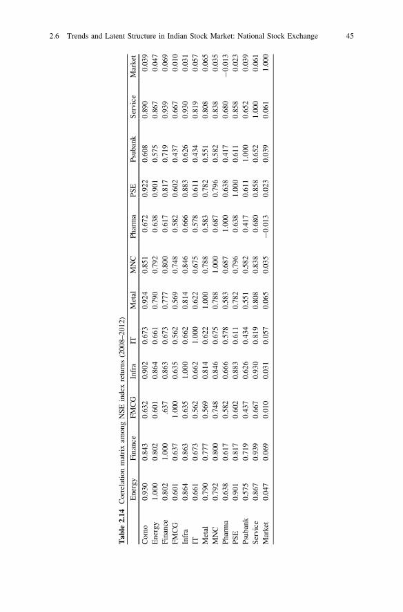
Tab

le2.

14C

orre

lati

onm

atri

xam

ong

NS

Ein

dex

retu

rns

(200

8–20

12)

Ene

rgy

Fin

ance

FM

CG

Infr

aIT

Met

alM

NC

Pha

rma

PS

EP

suba

nkS

ervi

ceM

arke

t

Com

o0.

930

0.84

30.

632

0.90

20.

673

0.92

40.

851

0.67

20.

922

0.60

80.

890

0.03

9E

nerg

y1.

000

0.80

20.

601

0.86

40.

661

0.79

00.

792

0.63

80.

901

0.57

50.

867

0.04

7F

inan

ce0.

802

1.00

0.6

370.

863

0.67

30.

777

0.80

00.

617

0.81

70.

719

0.93

90.

069

FM

CG

0.60

10.

637

1.00

00.

635

0.56

20.

569

0.74

80.

582

0.60

20.

437

0.66

70.

010

Infr

a0.

864

0.86

30.

635

1.00

00.

662

0.81

40.

846

0.66

60.

883

0.62

60.

930

0.03

1IT

0.66

10.

673

0.56

20.

662

1.00

00.

622

0.67

50.

578

0.61

10.

434

0.81

90.

057

Met

al0.

790

0.77

70.

569

0.81

40.

622

1.00

00.

788

0.58

30.

782

0.55

10.

808

0.06

5M

NC

0.79

20.

800

0.74

80.

846

0.67

50.

788

1.00

00.

687

0.79

60.

582

0.83

80.

035

Pha

rma

0.63

80.

617

0.58

20.

666

0.57

80.

583

0.68

71.

000

0.63

80.

417

0.68

0-

0.01

3P

SE

0.90

10.

817

0.60

20.

883

0.61

10.

782

0.79

60.

638

1.00

00.

611

0.85

80.

023

Psu

bank

0.57

50.

719

0.43

70.

626

0.43

40.

551

0.58

20.

417

0.61

11.

000

0.65

20.

039

Ser

vice

0.86

70.

939

0.66

70.

930

0.81

90.

808

0.83

80.

680

0.85

80.

652

1.00

00.

061

Mar

ket

0.04

70.

069

0.01

00.

031

0.05

70.

065

0.03

5-

0.01

30.

023

0.03

90.

061

1.00

0


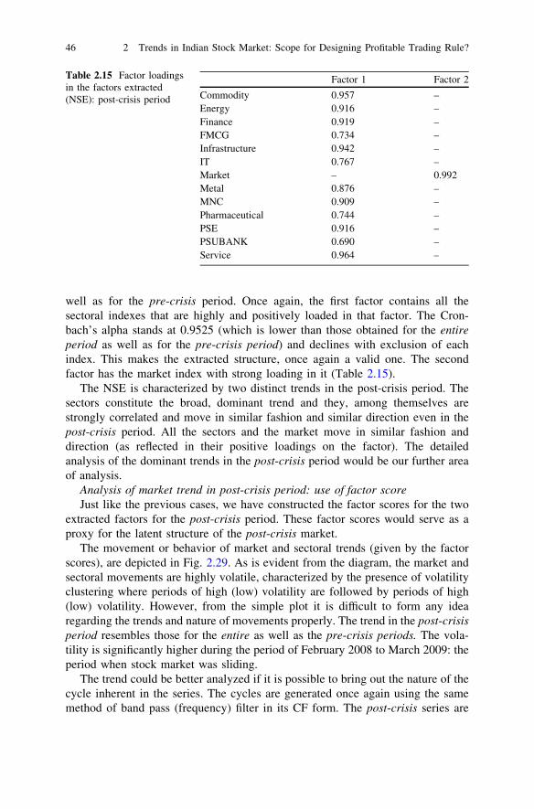
well as for the pre-crisis period. Once again, the first factor contains all thesectoral indexes that are highly and positively loaded in that factor. The Cron-bach’s alpha stands at 0.9525 (which is lower than those obtained for the entireperiod as well as for the pre-crisis period) and declines with exclusion of eachindex. This makes the extracted structure, once again a valid one. The secondfactor has the market index with strong loading in it (Table 2.15).

The NSE is characterized by two distinct trends in the post-crisis period. Thesectors constitute the broad, dominant trend and they, among themselves arestrongly correlated and move in similar fashion and similar direction even in thepost-crisis period. All the sectors and the market move in similar fashion anddirection (as reflected in their positive loadings on the factor). The detailedanalysis of the dominant trends in the post-crisis period would be our further areaof analysis.

Analysis of market trend in post-crisis period: use of factor scoreJust like the previous cases, we have constructed the factor scores for the two

extracted factors for the post-crisis period. These factor scores would serve as aproxy for the latent structure of the post-crisis market.

The movement or behavior of market and sectoral trends (given by the factorscores), are depicted in Fig. 2.29. As is evident from the diagram, the market andsectoral movements are highly volatile, characterized by the presence of volatilityclustering where periods of high (low) volatility are followed by periods of high(low) volatility. However, from the simple plot it is difficult to form any idearegarding the trends and nature of movements properly. The trend in the post-crisisperiod resembles those for the entire as well as the pre-crisis periods. The vola-tility is significantly higher during the period of February 2008 to March 2009: theperiod when stock market was sliding.

The trend could be better analyzed if it is possible to bring out the nature of thecycle inherent in the series. The cycles are generated once again using the samemethod of band pass (frequency) filter in its CF form. The post-crisis series are

Table 2.15 Factor loadingsin the factors extracted(NSE): post-crisis period

Factor 1 Factor 2

Commodity 0.957 –Energy 0.916 –Finance 0.919 –FMCG 0.734 –Infrastructure 0.942 –IT 0.767 –Market – 0.992Metal 0.876 –MNC 0.909 –Pharmaceutical 0.744 –PSE 0.916 –PSUBANK 0.690 –Service 0.964 –


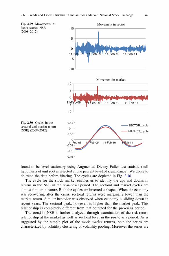
found to be level stationary using Augmented Dickey Fuller test statistic (nullhypothesis of unit root is rejected at one percent level of significance). We chose tode-trend the data before filtering. The cycles are depicted in Fig. 2.30.

The cycle for the stock market enables us to identify the ups and downs inreturns in the NSE in the post-crisis period. The sectoral and market cycles arealmost similar in nature. Both the cycles are inverted u-shaped. When the economywas recovering after the crisis, sectoral returns were marginally lower than themarket return. Similar behavior was observed when economy is sliding down inrecent years. The sectoral peak, however, is higher than the market peak. Thisrelationship is completely different from that obtained for the pre-crisis period.

The trend in NSE is further analyzed through examination of the risk-returnrelationship at the market as well as sectoral level in the post-crisis period. As issuggested by the simple plot of the stock market returns, both the series arecharacterized by volatility clustering or volatility pooling. Moreover the series are

-10

-5

0

5

10

11-Feb-08 11-Feb-09 11-Feb-10 11-Feb-11

Movement in sector

-10

-5

0

5

10

11-Feb-08 11-Feb-09 11-Feb-10 11-Feb-11

Movement in market

Fig. 2.29 Movements infactor scores, NSE(2008–2012)

-0.15

-0.1

-0.05

0

0.05

0.1

0.15

11-Feb-08 11-Feb-09 11-Feb-10 11-Feb-11

SECTOR_cycle

MARKET_cycle

Fig. 2.30 Cycles in thesectoral and market return(NSE) (2008–2012)


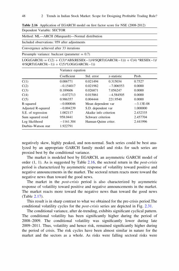
negatively skew, highly peaked, and non-normal. Such series could be best ana-lyzed by an appropriate GARCH family model and risks for such series areproxied best by the conditional variance.

The market is modeled best by EGARCH, an asymmetric GARCH model oforder (1, 1). As is suggested by Table 2.16, the sectoral return in the post-crisisperiod is characterized by asymmetric response of volatility toward positive andnegative announcements in the market. The sectoral return reacts more toward thenegative news than toward the good news.

The market in the post-crisis period is also characterized by asymmetricresponse of volatility toward positive and negative announcements in the market.The market reacts more toward the negative news than toward the good news(Table 2.17).

This result is in sharp contrast to what we obtained for the pre-crisis period.Theconditional volatility cycles for the post-crisis series are depicted in Fig. 2.31.

The conditional variance, after de-trending, exhibits significant cyclical pattern.The conditional volatility has been significantly higher during the period of2008–2009. The conditional volatility was significantly lower during late2009–2011. Thus, volatility and hence risk, remained significantly higher duringthe period of crisis. The risk cycles have been almost similar in nature for themarket and the sectors as a whole. As risks were falling sectoral risks were

Table 2.16 Application of EGARCH model on first factor score for NSE (2008-2012)

Dependent Variable: SECTOR

Method: ML—ARCH (Marquardt)—Normal distribution





Variance equation


C(1) 0.006771 0.021494 0.315034 0.7527C(2) -0.154017 0.021982 -7.006553 0.0000C(3) 0.189606 0.026871 7.056247 0.0000C(4) -0.072713 0.015861 -4.584505 0.0000C(5) 0.986357 0.004444 221.9540 0.0000R-squared -0.000046 Mean dependent var -3.13E-08Adjusted R-squared -0.004239 S.D. dependent var 1.000000S.E. of regression 1.002117 Akaike info criterion 2.432335Sum squared resid 958.0441 Schwarz criterion 2.457704Log likelihood -1161.304 Hannan-Quinn criter. 2.441996Durbin–Watson stat 1.922791


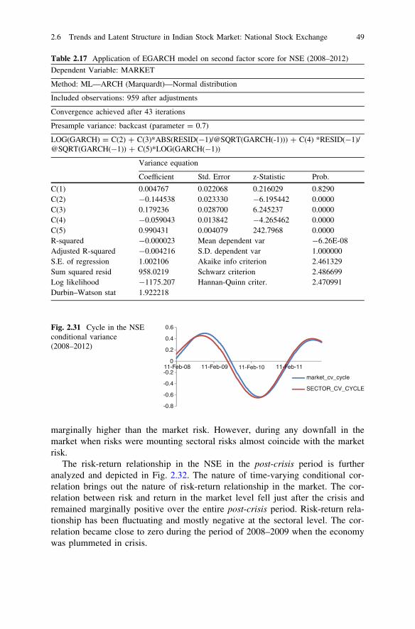
marginally higher than the market risk. However, during any downfall in themarket when risks were mounting sectoral risks almost coincide with the marketrisk.

The risk-return relationship in the NSE in the post-crisis period is furtheranalyzed and depicted in Fig. 2.32. The nature of time-varying conditional cor-relation brings out the nature of risk-return relationship in the market. The cor-relation between risk and return in the market level fell just after the crisis andremained marginally positive over the entire post-crisis period. Risk-return rela-tionship has been fluctuating and mostly negative at the sectoral level. The cor-relation became close to zero during the period of 2008–2009 when the economywas plummeted in crisis.

Table 2.17 Application of EGARCH model on second factor score for NSE (2008–2012)

Dependent Variable: MARKET

Method: ML—ARCH (Marquardt)—Normal distribution





Variance equation

Coefficient Std. Error z-Statistic Prob.

C(1) 0.004767 0.022068 0.216029 0.8290C(2) -0.144538 0.023330 -6.195442 0.0000C(3) 0.179236 0.028700 6.245237 0.0000C(4) -0.059043 0.013842 -4.265462 0.0000C(5) 0.990431 0.004079 242.7968 0.0000R-squared -0.000023 Mean dependent var -6.26E-08Adjusted R-squared -0.004216 S.D. dependent var 1.000000S.E. of regression 1.002106 Akaike info criterion 2.461329Sum squared resid 958.0219 Schwarz criterion 2.486699Log likelihood -1175.207 Hannan-Quinn criter. 2.470991Durbin–Watson stat 1.922218

-0.8

-0.6

-0.4

-0.2

0

0.2

0.4

0.6

11-Feb-08 11-Feb-09 11-Feb-10 11-Feb-11

market_cv_cycle

SECTOR_CV_CYCLE

Fig. 2.31 Cycle in the NSEconditional variance(2008–2012)


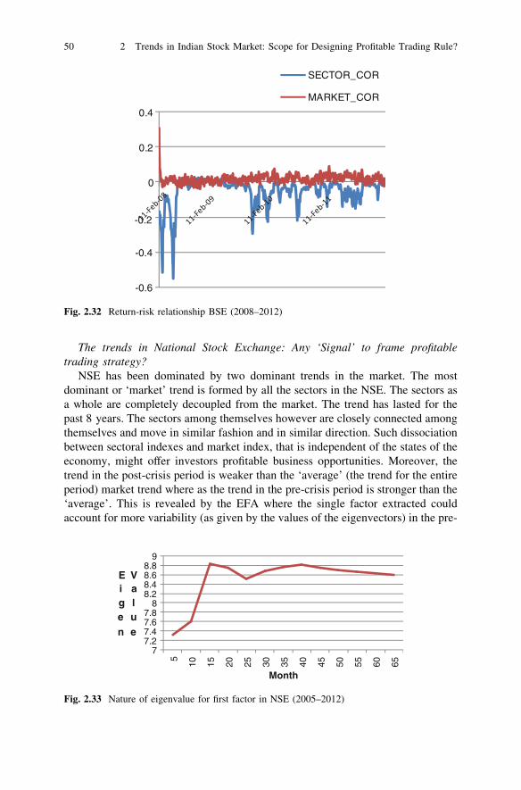
The trends in National Stock Exchange: Any ‘Signal’ to frame profitabletrading strategy?

NSE has been dominated by two dominant trends in the market. The mostdominant or ‘market’ trend is formed by all the sectors in the NSE. The sectors asa whole are completely decoupled from the market. The trend has lasted for thepast 8 years. The sectors among themselves however are closely connected amongthemselves and move in similar fashion and in similar direction. Such dissociationbetween sectoral indexes and market index, that is independent of the states of theeconomy, might offer investors profitable business opportunities. Moreover, thetrend in the post-crisis period is weaker than the ‘average’ (the trend for the entireperiod) market trend where as the trend in the pre-crisis period is stronger than the‘average’. This is revealed by the EFA where the single factor extracted couldaccount for more variability (as given by the values of the eigenvectors) in the pre-

-0.6

-0.4

-0.2

0

0.2

0.4

SECTOR_COR

MARKET_COR


77.27.47.67.8

88.28.48.68.8

9

5

10 15 20 25 30 35 40 45 50 55 60 65

Eigen

Value

Month

Fig. 2.33 Nature of eigenvalue for first factor in NSE (2005–2012)


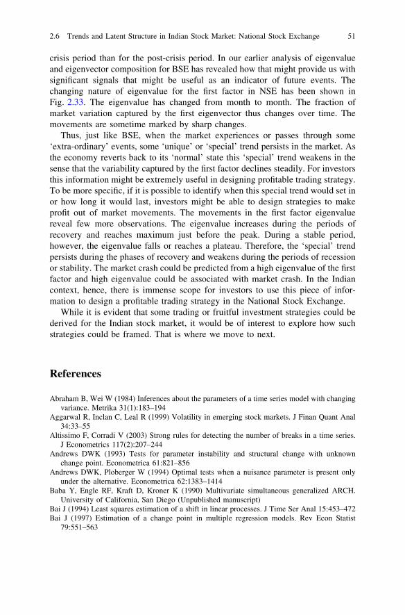
crisis period than for the post-crisis period. In our earlier analysis of eigenvalueand eigenvector composition for BSE has revealed how that might provide us withsignificant signals that might be useful as an indicator of future events. Thechanging nature of eigenvalue for the first factor in NSE has been shown inFig. 2.33. The eigenvalue has changed from month to month. The fraction ofmarket variation captured by the first eigenvector thus changes over time. Themovements are sometime marked by sharp changes.

Thus, just like BSE, when the market experiences or passes through some‘extra-ordinary’ events, some ‘unique’ or ‘special’ trend persists in the market. Asthe economy reverts back to its ‘normal’ state this ‘special’ trend weakens in thesense that the variability captured by the first factor declines steadily. For investorsthis information might be extremely useful in designing profitable trading strategy.To be more specific, if it is possible to identify when this special trend would set inor how long it would last, investors might be able to design strategies to makeprofit out of market movements. The movements in the first factor eigenvaluereveal few more observations. The eigenvalue increases during the periods ofrecovery and reaches maximum just before the peak. During a stable period,however, the eigenvalue falls or reaches a plateau. Therefore, the ‘special’ trendpersists during the phases of recovery and weakens during the periods of recessionor stability. The market crash could be predicted from a high eigenvalue of the firstfactor and high eigenvalue could be associated with market crash. In the Indiancontext, hence, there is immense scope for investors to use this piece of infor-mation to design a profitable trading strategy in the National Stock Exchange.

While it is evident that some trading or fruitful investment strategies could bederived for the Indian stock market, it would be of interest to explore how suchstrategies could be framed. That is where we move to next.

References

Abraham B, Wei W (1984) Inferences about the parameters of a time series model with changingvariance. Metrika 31(1):183–194

Aggarwal R, Inclan C, Leal R (1999) Volatility in emerging stock markets. J Finan Quant Anal34:33–55

Altissimo F, Corradi V (2003) Strong rules for detecting the number of breaks in a time series.J Econometrics 117(2):207–244

Andrews DWK (1993) Tests for parameter instability and structural change with unknownchange point. Econometrica 61:821–856

Andrews DWK, Ploberger W (1994) Optimal tests when a nuisance parameter is present onlyunder the alternative. Econometrica 62:1383–1414

Baba Y, Engle RF, Kraft D, Kroner K (1990) Multivariate simultaneous generalized ARCH.University of California, San Diego (Unpublished manuscript)

Bai J (1994) Least squares estimation of a shift in linear processes. J Time Ser Anal 15:453–472Bai J (1997) Estimation of a change point in multiple regression models. Rev Econ Statist

79:551–563


Bai J, Perron P (2003) Computation and analysis of multiple structural change models. J ApplEconom 18(1):1–22

Banerjee A, Lumsdaine RL, Stock JH (1992) Recursive and sequential tests of the unit root andtrend break hypotheses: theory and international evidence. J Bus Econ Statist 10:271–287

Baufays P, Rasson JP (1985) Variance changes in autoregressive models. In: Anderson OD (ed)Time series analysis: theory and practice, 7th edn. North Holland, New York

Bollerslev T, Engle RF, Wooldridge JM (1988) A capital asset pricing model with time varyingcovariances. J Pol Econ 96(1):116–131

Brooks C, Henry OT (2000) Linear and non-linear transmission of equity return volatility:evidence from the US, Japan and Australia. Econ Model 17:497–513

Cheng T (2009) An efficient algorithm for estimating a change-point. Stat Probabil Lett79:559–565

Chu CSJ, White H (1992) A direct test for changing trend. J Bus Econ Statist 10:189–199Gonzalo J, Pitarakis JY (2002) Estimation and model selection based inference in single and

multiple threshold models. J Econometrics 110:319–352Gregory AW, Hansen BE (1996) Residual-based tests for cointegration in the models with regime

shifts. J Econometrics 70:99–126Hair JF, Black WC, Babin BJ, Anderson R (2010) Multivariate data analysis, 7th edn. Pearson

Education Inc, IndiaHansen BE (1990) Lagrange multiplier tests for parameter instability in non-linear models.

Unpublished manuscript, University of Rochester, Rochester, New York. http://www.ssc.wisc.edu/*bhansen/paper/LMTests.pdf. Accessed 21 Sept 2010

Hansen BE (1992) Test for Instability with I(1) processes. J Bus Econ Statist 10:321–335Hansen BE (2001) The new econometrics of structural change: dating breaks in U.S. labor

productivity. J Econ Perspect 15(4):117–128Hsu A, Miller RB, Wichern DW (1974) On the stable Paretian behavior of stock-market prices.

J Am Statistical Assoc 69(345):108–113Huang B, Yang C (2001) The impact of settlement time on the volatility of stock market

revisited: an application of the iterated cumulative sums of squares detection method forchanges of variance. Appl Econ Lett 8:665–668

Inclan C, Tiao GC (1994) Use of cumulative sums of squares for retrospective detection ofchanges of variance. J Am Statistical Assoc 89:913–923

Ismail MT, Isa Z (2006) Modelling exchange rates using regime switching models. SainsMalaysiana 35(2):55–62

Karunanayake I, Valadkhani A, O’Brien M (2008) Modelling Australian stock market volatility:a multivariate GARCH approach. Economics Working Paper series, University of Wollon-gong, http://www.uow.edu.au/commerce/econ/wpapers.html, Accessed on 12 Aug 2010

Lumsdaine RL, Papell DH (1997) Multiple trend breaks and the unit root hypothesis. Rev EconStatist 79:223–230

Marcucci J (2005) Forecasting stock market volatility with regime-switching GARCH models.Stud Nonlinear 9(4). Dynam Econometrics 9(4):1–53 (Article 6)

Nelson CR, Plosser CI (1982) Trends and random walks in macroeconomic time series. J MonetEcon 10:139–162

Perron P (1989) The great crash, the oil-price shock and the unit-root hypothesis. Econometrica57:1361–1401

Perron P (1990) Testing for a unit root in a time series with a changing mean. J Bus Econ Statist8:153–162

Perron P (1997a) Further evidence on breaking trend functions in macroeconomic variables.J Econometrics 80(2):355–385

Perron P (1997b) L’estimation de Modèles avec Changements Structurels Multiples. L’ActualEcon 73(1):457–505

Perron P, Vogelsang TJ (1992) Nonstationarity and level shifts with an application to purchasingpower parity. J Bus Econ Statist 10:301–320


http://www.ssc.wisc.edu/~bhansen/paper/LMTests.pdf

http://www.ssc.wisc.edu/~bhansen/paper/LMTests.pdf

http://www.uow.edu.au/commerce/econ/wpapers.html

Sansó A, Aragó V, Carrion-i-Silvestre JLl (2004) Testing for Changes in the UnconditionalVariance of Financial Time Series. Revista Econ Financiera 4:32–53

Schaller H, Norden SV (1997) Regime switching in stock market returns. Appl Finan Econ7(2):177–191

Scherrer W, Ribarits E (2007) On the parameterization of multivariate GARCH models.Econometric Theory 23:464–484

Tsay RS (1988) Outliers, level shifts and variance changes in time series. J Forecast 7:1–20Valentinyi-Endrész M (2004) Structural breaks and financial risk management. MNB Working

Papers 2004/11, Magyar Nemzeti Bank, The Central Bank of Hungary. http://english.mnb.hu/Root/Dokumentumtar/ENMNB/Kiadvanyok/mnben_mnbfuzetek/mnben_wp200411/wp2004_11v.pdf. Accessed 2 January 2009

Wilson B, Aggarwal R, Inclan C (1996) Detecting volatility changes across the oil sector.J Futures Markets 16:313–330

Zivot E, Andrews DWK (1992) Further evidence on the great crash, the oil price shock, and theunit-root hypothesis. J Bus Econ Statist 10:251–270

References 53

http://english.mnb.hu/Root/Dokumentumtar/ENMNB/Kiadvanyok/mnben_mnbfuzetek/mnben_wp200411/wp2004_11v.pdf



Documents

Chapter 2 Trends in Indian Stock Market: Scope for