Chapter 200 Descriptive Statistics - · PDF fileChapter 200 Descriptive Statistics Introduction This procedure summarizes variables both statistically and graphically. ... A kurtosis

NCSS Statistical Software NCSS.com

200-1 © NCSS, LLC. All Rights Reserved.

Chapter 200

Descriptive Statistics Introduction This procedure summarizes variables both statistically and graphically. Information about the location (center), spread (variability), and distribution is provided. The procedure provides a large variety of statistical information about a single variable.

Kinds of Research Questions The use of this module for a single variable is generally appropriate for one of four purposes: numerical summary, data screening, outlier identification (which sometimes is incorporated into data screening), and distributional shape. We will briefly discuss each of these now.

Numerical Descriptors The numerical descriptors of a sample are called statistics. These statistics may be categorized as location, spread, shape indicators, percentiles, and interval estimates.

Location or Central Tendency One of the first impressions that we like to get from a variable is its general location. You might think of this as the center of the variable on the number line. The average (mean) is a common measure of location. When investigating the center of a variable, the main descriptors are the mean, median, mode, and the trimmed mean. Other averages, such as the geometric and harmonic mean, have specialized uses. We will now briefly compare these measures.

If the data come from the normal distribution, the mean, median, mode, and the trimmed mean are all equal. If the mean and median are very different, most likely there are outliers in the data or the distribution is skewed. If this is the case, the median is probably a better measure of location. The mean is very sensitive to extreme values and can be seriously contaminated by just one observation.

A compromise between the mean and median is given by the trimmed mean (where a predetermined number of observations are trimmed from each end of the data distribution). This trimmed mean is more robust than the mean but more sensitive than the median. Comparison of the trimmed mean to the median should show the trimmed mean approaching the median as the degree of trimming increases. If the trimmed mean converges to the median for a small degree of trimming, say 5 or 10%, the number of outliers is relatively few.

http://www.ncss.com/

NCSS Statistical Software NCSS.com Descriptive Statistics


Variability, Dispersion, or Spread After establishing the center of a variable’s values, the next question is how closely the data fall about this center. The pattern of the values around the center is called the spread, dispersion, or variability. There are numerous measures of variability: range, variance, standard deviation, interquartile range, and so on. All of these measures of dispersion are affected by outliers to some degree, but some do much better than others.

The standard deviation is one of the most popular measures of dispersion. Unfortunately, it is greatly influenced by outlying observations and by the overall shape of the distribution. Because of this, various substitutes for it have been developed. It will be up to you to decide which is best in a given situation.

Shape The shape of the distribution describes the pattern of the values along the number line. Are there a few unique values that occur over and over, or is there a continuum? Is the pattern symmetric or asymmetric? Are the data bell shaped? Do they seem to have a single center or are there several areas of clumping? These are all aspects of the shape of the distribution of the data.

Two of the most popular measures of shape are skewness and kurtosis. Skewness measures the direction and lack of symmetry. The more skewed a distribution is, the greater the need for using robust estimators, such as the median and the interquartile range. Positive skewness indicates a longtailedness to the right while negative skewness indicates longtailedness to the left. Kurtosis measures the heaviness of the tails. A kurtosis value less than three indicates lighter tails than a normal distribution. Kurtosis values greater than three indicate heavier tails than a normal distribution.

The measures of shape require more data to be accurate. For example, a reasonable estimate of the mean may require only ten observations in a random sample. The standard deviation will require at least thirty. A reasonably detailed estimate of the shape (especially if the tails are important) will require several hundred observations.

Percentiles Percentiles are extremely useful for certain applications as well as for cases when the distribution is very skewed or contaminated by outliers. If the distribution of the variable is skewed, you might want to use the exact interval estimates for the percentiles.

Confidence Limits or Interval Estimates An interval estimate of a statistic gives a range of its possible values. Confidence limits are a special type of interval estimate that have, under certain conditions, a level of confidence or probability attached to them.

If the assumption of normality is valid, the confidence intervals for the mean, variance, and standard deviation are valid. However, the standard error of each of these intervals depends on the sample standard deviation and the sample size. If the sample standard deviation is inaccurate, these other measures will be also. The bottom line is that outliers not only affect the standard deviation but also all confidence limits that use the sample standard deviation. It should be obvious then that the standard deviation is a critical measure of dispersion in parametric methods.




Data Screening Data screening involves missing data, data validity, and outliers. If these issues are not dealt with prior to the use of descriptive statistics, errors in interpretations are very likely.

Missing Data Whenever data are missing, questions need to be asked.

1. Is the missingness due to incomplete data collection? If so, try to complete the data collection.

2. Is the missingness due to nonresponse from a survey? If so, attempt to collect data from the nonresponders.

3. Are the missing data due to a censoring of data beyond or below certain values? If so, some different statistical tools will be needed.

4. Is the pattern of missingness random? If only a few data points are missing from a large data set and the pattern of missingness is random, there is little to be concerned with. However, if the data set is small or moderate in size, any degree of missingness could cause bias in interpretations.

Whenever missing values occur without answers to the above questions, there is little that can be done. If the distributional shape of the variable is known and there are missing data for certain percentiles, estimates could be made for the missing values. If there are other variables in the data set as well and the pattern of missingness is random, multiple regression and multivariate methods can be used to estimate the missing values.

Data Validity Data validity needs to be confirmed prior to any statistical analysis, but it usually begins after a univariate descriptive analysis. Extremes or outliers for a variable could be due to a data entry error, to an incorrect or inappropriate specification of a missing code, to sampling from a population other than the intended one, or due to a natural abnormality that exists in this variable from time to time. The first two cases of invalid data are easily corrected. The latter two require information about the distribution form and necessitate the use of regression or multivariate methods to re-estimate the values.

Outliers Outliers in a univariate data set are defined as observations that appear to be inconsistent with the rest of the data. An outlier is an observation that sticks out at either end of the data set.

The visualization of univariate outliers can be done in three ways: with the stem-and-leaf plot, with the box plot, and with the normal probability plot. In each of these informal methods, the outlier is far removed from the rest of the data. A word of caution: the box plot and the normal probability plot evaluate the potentiality of an outlier assuming the data are normally distributed. If the variable is not normally distributed, these plots may indicate many outliers. You must be careful about checking what distributional assumptions are behind the outliers you may be looking for.

Outliers can completely distort descriptive statistics. For instance, if one suspects outliers, a comparison of the mean, median, mode, and trimmed mean should be made. If the outliers are only to one side of the mean, the median is a better measure of location. On the other hand, if the outliers are equally divergent on each side of the center, the mean and median will be close together, but the standard deviation will be inflated. The interquartile range is the only measure of variation not greatly affected by outliers. Outliers may also contaminate measures of skewness and kurtosis as well as confidence limits.

This discussion has focused on univariate outliers, in a simplistic way. If the data set has several variables, multiple regression and multivariate methods must be used to identify these outliers.




Normality A primary use of descriptive statistics is to determine whether the data are normally distributed. If the variable is normally distributed, you can use parametric statistics that are based on this assumption. If the variable is not normally distributed, you might try a transformation on the variable (such as, the natural log or square root) to make the data normal. If a transformation is not a viable alternative, nonparametric methods that do not require normality should be used.

NCSS provides seven tests to formally test for normality. If a variable fails a normality test, it is critical to look at the box plot and the normal probability plot to see if an outlier or a small subset of outliers has caused the nonnormality. A pragmatic approach is to omit the outliers and rerun the tests to see if the variable now passes the normality tests.

Always remember that a reasonably large sample size is necessary to detect normality. Only extreme types of nonnormality can be detected with samples less than fifty observations.

There is a common misconception that a histogram is always a valid graphical tool for assessing normality. Since there are many subjective choices that must be made in constructing a histogram, and since histograms generally need large sample sizes to display an accurate picture of normality, preference should be given to other graphical displays such as the box plot, the density trace, and the normal probability plot.

Data Structure The data are contained in a single variable.

Height dataset (subset)

Height 64 63 67 . . .

Procedure Options This section describes the options available in this procedure. To find out more about using a procedure, turn to the Procedures chapter.

Following is a list of the procedure’s options.

Variables Tab The options on this panel specify which variables to use.

Data Variables

Variable(s) Specify a list of one or more variables upon which the univariate statistics are to be generated. You can double-click the field or single click the button on the right of the field to bring up the Variable Selection window.




Frequency Variable

Frequency Variable This optional variable specifies the number of observations that each row represents. When omitted, each row represents a single observation. If your data is the result of a previous summarization, you may want certain rows to represent several observations. Note that negative values are treated as a zero weight and are omitted. This is one way of weighting your data.

Grouping Variables

Group (1-5) Variable You can select up to five categorical variables. When one or more of these are specified, a separate set of reports is generated for each unique set of values for these variables.

Data Transformation Options

Exponent Occasionally, you might want to obtain a statistical report on the square root or square of your variable. This option lets you specify an on-the-fly transformation of the variable. The form of this transformation is X = YA, where Y is the original value, A is the selected exponent, and X is the value that is summarized.

Additive Constant Occasionally, you might want to obtain a statistical report on a transformed version of a variable. This option lets you specify an on-the-fly transformation of the variable. The form of this transformation is X = Y+B, where Y is the original value, B is the selected value, and X is the value that is summarized.

Note that if you apply both the Exponent and the Additive Constant, the form of the transformation is X = (Y+B)A.

Reports Tab The options on this panel control the format of the report.

Select Reports

Summary Section … Percentile Section Each of these options indicates whether to display the indicated report.

Alpha Level The value of alpha for the confidence limits and rejection decisions. Usually, this number will range from 0.1 to 0.001. The default value of 0.05 results in 95% confidence limits.

Stem and Leaf

Stem Leaf Specify whether to include the stem and leaf plot.




Report Options

Precision Specify the precision of numbers in the report. A single-precision number will show seven-place accuracy, while a double-precision number will show thirteen-place accuracy. Note that the reports were formatted for single precision. If you select double precision, some numbers may run into others. Also note that all calculations are performed in double precision regardless of which option you select here. This is for reporting purposes only.

Value Labels This option applies to the Group Variable(s). It lets you select whether to display data values, value labels, or both. Use this option if you want the output to automatically attach labels to the values (like 1=Yes, 2=No, etc.). See the section on specifying Value Labels elsewhere in this manual.

Variable Names This option lets you select whether to display only variable names, variable labels, or both.

Report Options - Decimal Places

Values, Means, Probabilities Specify the number of decimal places when displaying this item. Select ‘General’ to display all possible decimal places.

Report Options - Percentiles

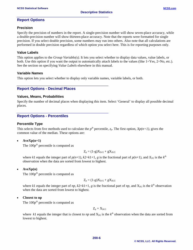
Percentile Type This selects from five methods used to calculate the pth percentile, zp. The first option, Xp(n+1), gives the common value of the median. These options are:

• AveXp(n+1) The 100pth percentile is computed as

Zp = (1-g)X[k1] + gX[k2]

where k1 equals the integer part of p(n+1), k2=k1+1, g is the fractional part of p(n+1), and X[k] is the kth observation when the data are sorted from lowest to highest.

• AveXp(n) The 100pth percentile is computed as

Zp = (1-g)X[k1] + gX[k2]

where k1 equals the integer part of np, k2=k1+1, g is the fractional part of np, and X[k] is the kth observation when the data are sorted from lowest to highest.

• Closest to np The 100pth percentile is computed as

Zp = X[k1]

where k1 equals the integer that is closest to np and X[k] is the kth observation when the data are sorted from lowest to highest.




• EDF The 100pth percentile is computed as

Zp = X[k1]

where k1 equals the integer part of np if np is exactly an integer or the integer part of np+1 if np is not exactly an integer. X[k] is the kth observation when the data are sorted from lowest to highest. Note that EDF stands for empirical distribution function.

• EDF w/Ave The 100pth percentile is computed as

Zp = (X[k1] + X[k2])/2

where k1 and k2 are defined as follows: If np is an integer, k1=k2=np. If np is not exactly an integer, k1 equals the integer part of np and k2 = k1+1. X[k] is the kth observation when the data are sorted from lowest to highest. Note that EDF stands for empirical distribution function.

• Smallest Percentile By default, the smallest percentile displayed is the 1st percentile. This option lets you change this value to any value between 0 and 100. For example, you might enter 2.5 to see the 2.5th percentile.

• Largest Percentile By default, the largest percentile displayed is the 99th percentile. This option lets you change this value to any value between 0 and 100. For example, you might enter 97.5 to see the 97.5th percentile.

Plots Tab These options specify the plots.

Select Plots

Histogram and Probability Plot Specify whether to display the indicated plots. Click the plot format button to change the plot settings.




Example 1 – Running Descriptive Statistics This section presents a detailed example of how to run a descriptive statistics report on the Height variable in the Height dataset. To run this example, take the following steps (note that step 1 is not necessary if the Height dataset is open):

You may follow along here by making the appropriate entries or load the completed template Example 1 by clicking on Open Example Template from the File menu of the Descriptive Statistics window.

1 Open the Height dataset. • From the File menu of the NCSS Data window, select Open Example Data. • Click on the file Height.NCSS. • Click Open.

2 Open the Descriptive Statistics window. • Using the Analysis menu or the Procedure Navigator, find and select the Descriptive Statistics

procedure. • On the menus, select File, then New Template. This will fill the procedure with the default template.

3 Specify the Height variable. • On the Descriptive Statistics window, select the Variables tab. (This is the default.) • Double-click in the Variables text box. This will bring up the variable selection window. • Select Height from the list of variables and then click Ok. The word “Height” will appear in the

Variables box. Remember that you could have entered a “1” here signifying the first (left-most) variable on the dataset.

4 Run the procedure. • From the Run menu, select Run Procedure. Alternatively, just click the green Run button.

The following reports and charts will be displayed in the Output window.

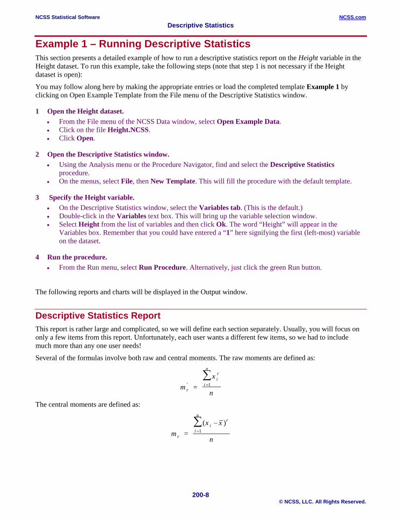
Descriptive Statistics Report This report is rather large and complicated, so we will define each section separately. Usually, you will focus on only a few items from this report. Unfortunately, each user wants a different few items, so we had to include much more than any one user needs!

Several of the formulas involve both raw and central moments. The raw moments are defined as:

mx

nr

ir

i

n

' = =∑

1

The central moments are defined as:

mx x

nr

ii

nr

= ( )

=∑ −

1




Large sample estimates of the standard errors are provided for several statistics. These are based on the following formula from Kendall and Stuart (1987):

Var m m m m m rm mnr

r r r r r( ) - - +=− + −2

22 1

21 14 2

Var g x dgdx

Var x( ( )) ( )=

2

Summary Section

Summary Section of Height Standard Standard Count Mean Deviation Error Minimum Maximum Range 20 62.1 8.441128 1.887493 51 79 28

Count This is the number of nonmissing values. If no frequency variable was specified, this is the number of nonmissing rows.

Mean This is the average of the data values. (See Means Section below.)

Standard Deviation This is the standard deviation of the data values. (See Variation Section below.)

Standard Error This is the standard error of the mean. (See Means Section below.)

Minimum The smallest value in this variable.

Maximum The largest value in this variable.

Range The difference between the largest and smallest values for a variable. If the data for a given variable is normally distributed, a quick estimate of the standard deviation can be made by dividing the range by six.

Count Section

Counts Section of Height Sum of Missing Distinct Total Adjusted Rows Frequencies Values Values Sum Sum Squares Sum Squares 75 20 55 14 1242 78482 1353.8

Rows This is the total number of rows available in this variable.




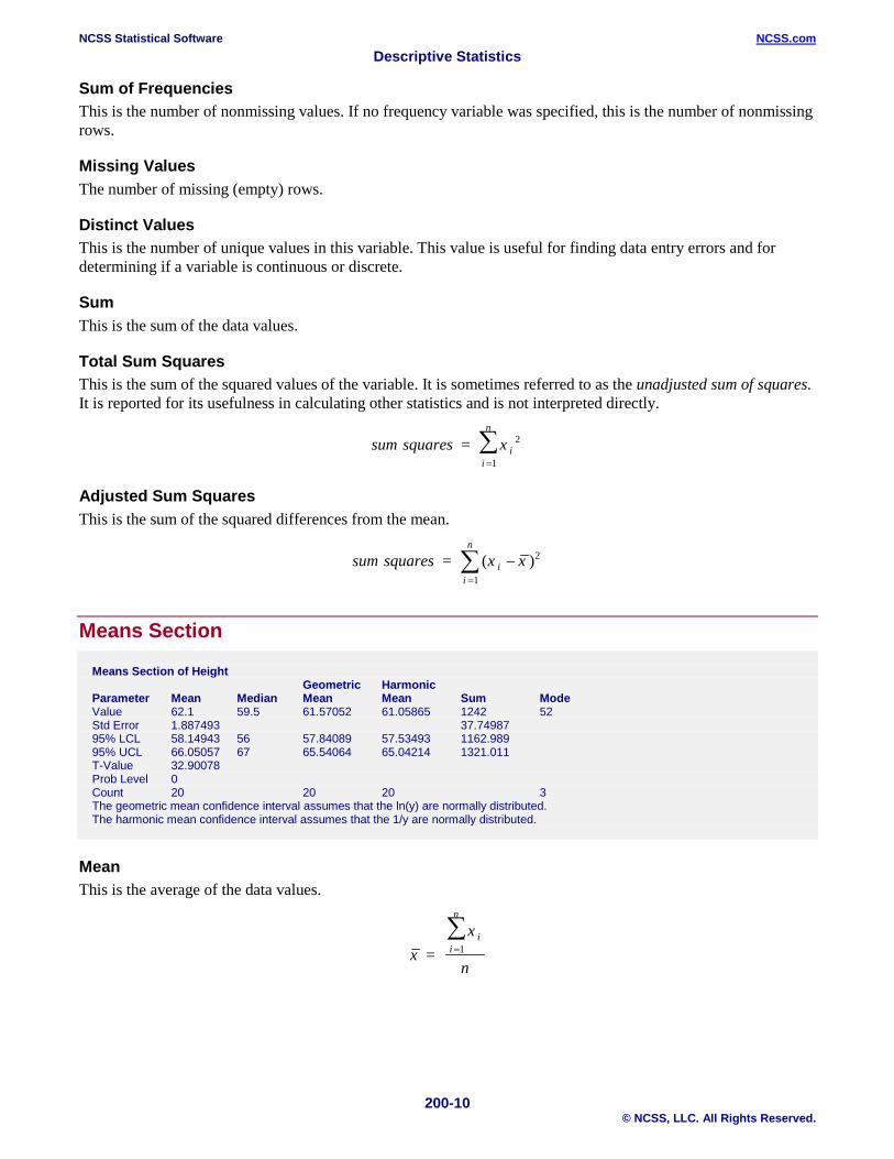
Sum of Frequencies This is the number of nonmissing values. If no frequency variable was specified, this is the number of nonmissing rows.

Missing Values The number of missing (empty) rows.

Distinct Values This is the number of unique values in this variable. This value is useful for finding data entry errors and for determining if a variable is continuous or discrete.

Sum This is the sum of the data values.

Total Sum Squares This is the sum of the squared values of the variable. It is sometimes referred to as the unadjusted sum of squares. It is reported for its usefulness in calculating other statistics and is not interpreted directly.

sum squares x ii

n

= 2

1=∑

Adjusted Sum Squares This is the sum of the squared differences from the mean.

sum squares x xii

n

= ( )−=∑ 2

1

Means Section

Means Section of Height Geometric Harmonic Parameter Mean Median Mean Mean Sum Mode Value 62.1 59.5 61.57052 61.05865 1242 52 Std Error 1.887493 37.74987 95% LCL 58.14943 56 57.84089 57.53493 1162.989 95% UCL 66.05057 67 65.54064 65.04214 1321.011 T-Value 32.90078 Prob Level 0 Count 20 20 20 3 The geometric mean confidence interval assumes that the ln(y) are normally distributed. The harmonic mean confidence interval assumes that the 1/y are normally distributed.

Mean This is the average of the data values.

xx

n

ii

n

= =∑

1




Std Error (Mean) This is the standard error of the mean. This is the estimated standard deviation for the distribution of sample means for an infinite population.

ssnx =

LCL and 95% UCL of the Mean This is the upper and lower values of a 100(1-α) interval estimate for the mean based on a t distribution with n-1 degrees of freedom. This interval estimate assumes that the population standard deviation is not known and that the data for this variable are normally distributed.

x t sa n x± −/ ,2 1

T-Value (Mean) This is the t-test value for testing that the sample mean is equal to zero versus the alternative that it is not. The degrees of freedom for this t-test are n-1. The variable that is being tested must be approximately normally distributed for this test to be valid.

t = x sn

xα / ,2 1−

Prob Level (Mean) This is the significance level of the above t-test, assuming a two-tailed test. Generally, this p-value is compared to the level of significance, .05 or .01, chosen by the researcher. If the p-value is less than the pre-determined level of significance, the sample mean is different from zero.

Median The value of the median. The median is the 50th percentile of the data set. It is the point that splits the data base in half. The value of the percentile depends upon the percentile method that was selected.

LCL and 95% UCL of the Median These are the values of an exact confidence interval for the median. These exact confidence intervals are discussed in the Percentile Section.

Geometric Mean The geometric mean (GM) is an alternative type of mean that is used for business, economic, and biological applications. Only nonnegative values are used in the computation. If one of the values is zero, the geometric mean is defined to be zero.

One example of when the GM is appropriate is when a variable is the product of many small effects combined by multiplication instead of addition.

GM = xii

n n

=∏

1

1/

An alternative form, showing the GM’s relationship to the arithmetic mean, is:

GM = n

xiexp ln( )1∑

Count for Geometric Mean The number of positive numbers used in computing the geometric mean.




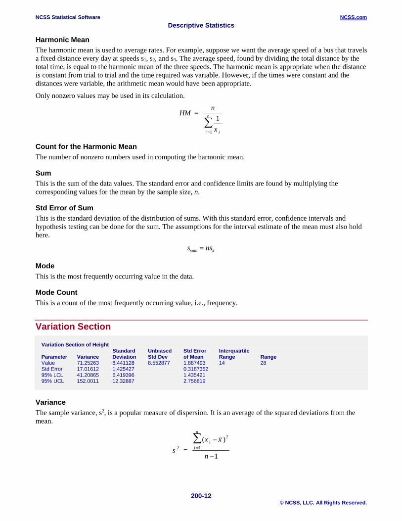
Harmonic Mean The harmonic mean is used to average rates. For example, suppose we want the average speed of a bus that travels a fixed distance every day at speeds s1, s2, and s3. The average speed, found by dividing the total distance by the total time, is equal to the harmonic mean of the three speeds. The harmonic mean is appropriate when the distance is constant from trial to trial and the time required was variable. However, if the times were constant and the distances were variable, the arithmetic mean would have been appropriate.

Only nonzero values may be used in its calculation.

HM = n

x ii

n 1

1=∑

Count for the Harmonic Mean The number of nonzero numbers used in computing the harmonic mean.

Sum This is the sum of the data values. The standard error and confidence limits are found by multiplying the corresponding values for the mean by the sample size, n.

Std Error of Sum This is the standard deviation of the distribution of sums. With this standard error, confidence intervals and hypothesis testing can be done for the sum. The assumptions for the interval estimate of the mean must also hold here.

Mode This is the most frequently occurring value in the data.

Mode Count This is a count of the most frequently occurring value, i.e., frequency.

Variation Section

Variation Section of Height Standard Unbiased Std Error Interquartile Parameter Variance Deviation Std Dev of Mean Range Range Value 71.25263 8.441128 8.552877 1.887493 14 28 Std Error 17.01612 1.425427 0.3187352 95% LCL 41.20865 6.419396 1.435421 95% UCL 152.0011 12.32887 2.756819

Variance The sample variance, s2, is a popular measure of dispersion. It is an average of the squared deviations from the mean.

sx x

n

ii

n

2 1

2

1 =

( )=∑ −

−

s nssum x=




Std Error of Variance This is a large sample estimate of the standard error of s2 for an infinite population.

LCL of the Variance This is the lower value of a 100(1-α) interval estimate for the variance based on the chi-squared distribution with n-1 degrees of freedom. This interval estimate assumes that the variable is normally distributed.

LCL = s (n - 1)2

/ 2 n2αχ , −1

UCL of the Variance This is the upper value of a 100(1-α) interval estimate for the variance based on the chi-squared distribution with n-1 degrees of freedom. This interval estimate assumes that the variable is normally distributed.

UCL = s (n - 1)2

/ 2 n21 1− −αχ ,

Standard Deviation The sample standard deviation, s, is a popular measure of dispersion. It measures the average distance between a single observation and its mean. The use of n-1 in the denominator instead of the more natural n is often of concern. It turns out that if n (instead of n-1) were used, a biased estimate of the population standard deviation would result. The use of n-1 corrects for this bias.

Unfortunately, s is inordinately influenced by outliers. For this reason, you must always check for outliers in your data before you use this statistic. Also, s is a biased estimator of the population standard deviation. An unbiased estimate, calculated by adjusting s, is given under the heading Unbiased Std Dev.

sx x

n

ii

n

= ( )

=∑ −

−1

2

1

Another form of the above formula that shows that the standard deviation is proportional to the difference between each pair of observations. Notice that the sample mean does not enter into this second formulation.

s

x x

n n

iall i j where i j

j

=

( ),

( )<

∑ −

−

2

1

Std Error of Standard Deviation This is a large sample estimate of the standard error of s for an infinite population.

LCL of Standard Deviation This is the lower value of a 100(1-α) interval estimate for the standard deviation based on the chi-squared distribution with n-1 degrees of freedom. This interval estimate assumes that the variable is normally distributed.

LCL = s (n - 1)2

/ 2 n2αχ , −1




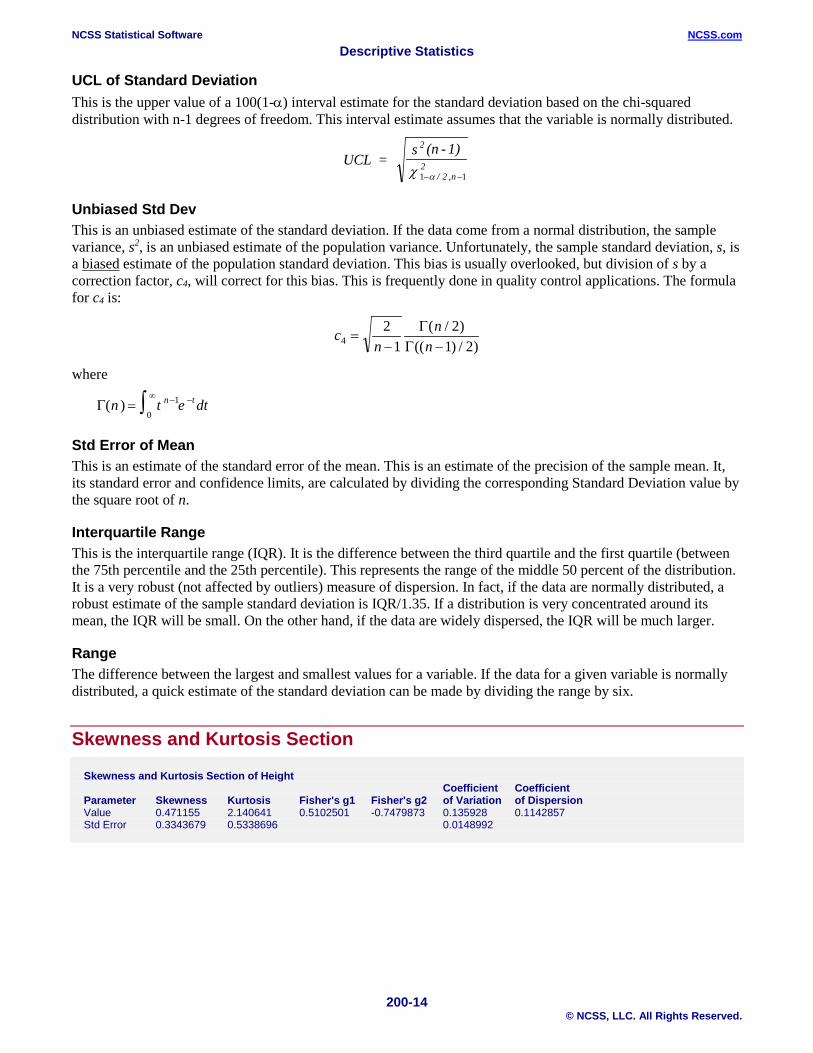
UCL of Standard Deviation This is the upper value of a 100(1-α) interval estimate for the standard deviation based on the chi-squared distribution with n-1 degrees of freedom. This interval estimate assumes that the variable is normally distributed.

UCL = s (n - 1)2

/ 2 n21 1− −αχ ,

Unbiased Std Dev This is an unbiased estimate of the standard deviation. If the data come from a normal distribution, the sample variance, s2, is an unbiased estimate of the population variance. Unfortunately, the sample standard deviation, s, is a biased estimate of the population standard deviation. This bias is usually overlooked, but division of s by a correction factor, c4, will correct for this bias. This is frequently done in quality control applications. The formula for c4 is:

cn

nn4

21

21 2

=− −

ΓΓ

( / )(( ) / )

where

Γ( )n t e dtn t= − −∞∫ 10

Std Error of Mean This is an estimate of the standard error of the mean. This is an estimate of the precision of the sample mean. It, its standard error and confidence limits, are calculated by dividing the corresponding Standard Deviation value by the square root of n.

Interquartile Range This is the interquartile range (IQR). It is the difference between the third quartile and the first quartile (between the 75th percentile and the 25th percentile). This represents the range of the middle 50 percent of the distribution. It is a very robust (not affected by outliers) measure of dispersion. In fact, if the data are normally distributed, a robust estimate of the sample standard deviation is IQR/1.35. If a distribution is very concentrated around its mean, the IQR will be small. On the other hand, if the data are widely dispersed, the IQR will be much larger.

Range The difference between the largest and smallest values for a variable. If the data for a given variable is normally distributed, a quick estimate of the standard deviation can be made by dividing the range by six.

Skewness and Kurtosis Section

Skewness and Kurtosis Section of Height Coefficient Coefficient Parameter Skewness Kurtosis Fisher's g1 Fisher's g2 of Variation of Dispersion Value 0.471155 2.140641 0.5102501 -0.7479873 0.135928 0.1142857 Std Error 0.3343679 0.5338696 0.0148992




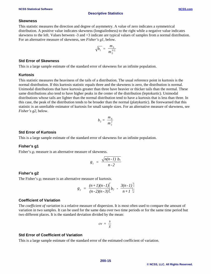
Skewness This statistic measures the direction and degree of asymmetry. A value of zero indicates a symmetrical distribution. A positive value indicates skewness (longtailedness) to the right while a negative value indicates skewness to the left. Values between -3 and +3 indicate are typical values of samples from a normal distribution. For an alternative measure of skewness, see Fisher’s g1, below.

bm

m1 / = 3

23 2

Std Error of Skewness This is a large sample estimate of the standard error of skewness for an infinite population.

Kurtosis This statistic measures the heaviness of the tails of a distribution. The usual reference point in kurtosis is the normal distribution. If this kurtosis statistic equals three and the skewness is zero, the distribution is normal. Unimodal distributions that have kurtosis greater than three have heavier or thicker tails than the normal. These same distributions also tend to have higher peaks in the center of the distribution (leptokurtic). Unimodal distributions whose tails are lighter than the normal distribution tend to have a kurtosis that is less than three. In this case, the peak of the distribution tends to be broader than the normal (platykurtic). Be forewarned that this statistic is an unreliable estimator of kurtosis for small sample sizes. For an alternative measure of skewness, see Fisher’s g2, below.

bmm2 = 4

22

Std Error of Kurtosis This is a large sample estimate of the standard error of skewness for an infinite population.

Fisher’s g1 Fisher’s g1 measure is an alternative measure of skewness.

11g =

n(n -1) bn - 2

Fisher’s g2 The Fisher’s g2 measure is an alternative measure of kurtosis.

2 2g = (n+1)(n -1)(n - 2)(n - 3) b -

3(n -1)n+1

Coefficient of Variation The coefficient of variation is a relative measure of dispersion. It is most often used to compare the amount of variation in two samples. It can be used for the same data over two time periods or for the same time period but two different places. It is the standard deviation divided by the mean:

cv = sx

Std Error of Coefficient of Variation This is a large sample estimate of the standard error of the estimated coefficient of variation.




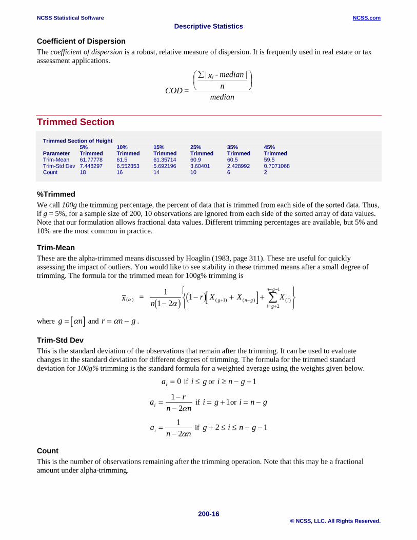
Coefficient of Dispersion The coefficient of dispersion is a robust, relative measure of dispersion. It is frequently used in real estate or tax assessment applications.

mediann

|median - x |

= COD

i

∑

Trimmed Section

Trimmed Section of Height 5% 10% 15% 25% 35% 45% Parameter Trimmed Trimmed Trimmed Trimmed Trimmed Trimmed Trim-Mean 61.77778 61.5 61.35714 60.9 60.5 59.5 Trim-Std Dev 7.448297 6.552353 5.692196 3.60401 2.428992 0.7071068 Count 18 16 14 10 6 2

%Trimmed We call 100g the trimming percentage, the percent of data that is trimmed from each side of the sorted data. Thus, if g = 5%, for a sample size of 200, 10 observations are ignored from each side of the sorted array of data values. Note that our formulation allows fractional data values. Different trimming percentages are available, but 5% and 10% are the most common in practice.

Trim-Mean These are the alpha-trimmed means discussed by Hoaglin (1983, page 311). These are useful for quickly assessing the impact of outliers. You would like to see stability in these trimmed means after a small degree of trimming. The formula for the trimmed mean for 100g% trimming is

( ) ( )[ ]( ) ( ) ( ) ( )α αx =

nr X X Xg n g i

i g

n g11 2

1 12

1

−− + +

+ −= +

− −

∑

where [ ]g n= α and r n g= −α .

Trim-Std Dev This is the standard deviation of the observations that remain after the trimming. It can be used to evaluate changes in the standard deviation for different degrees of trimming. The formula for the trimmed standard deviation for 100g% trimming is the standard formula for a weighted average using the weights given below.

ai = 0 if i g≤ or i n g≥ − +1

a rn ni =

−−1

2α if i g= +1or i n g= −

an ni = −

12α

if g i n g+ ≤ ≤ − −2 1

Count This is the number of observations remaining after the trimming operation. Note that this may be a fractional amount under alpha-trimming.




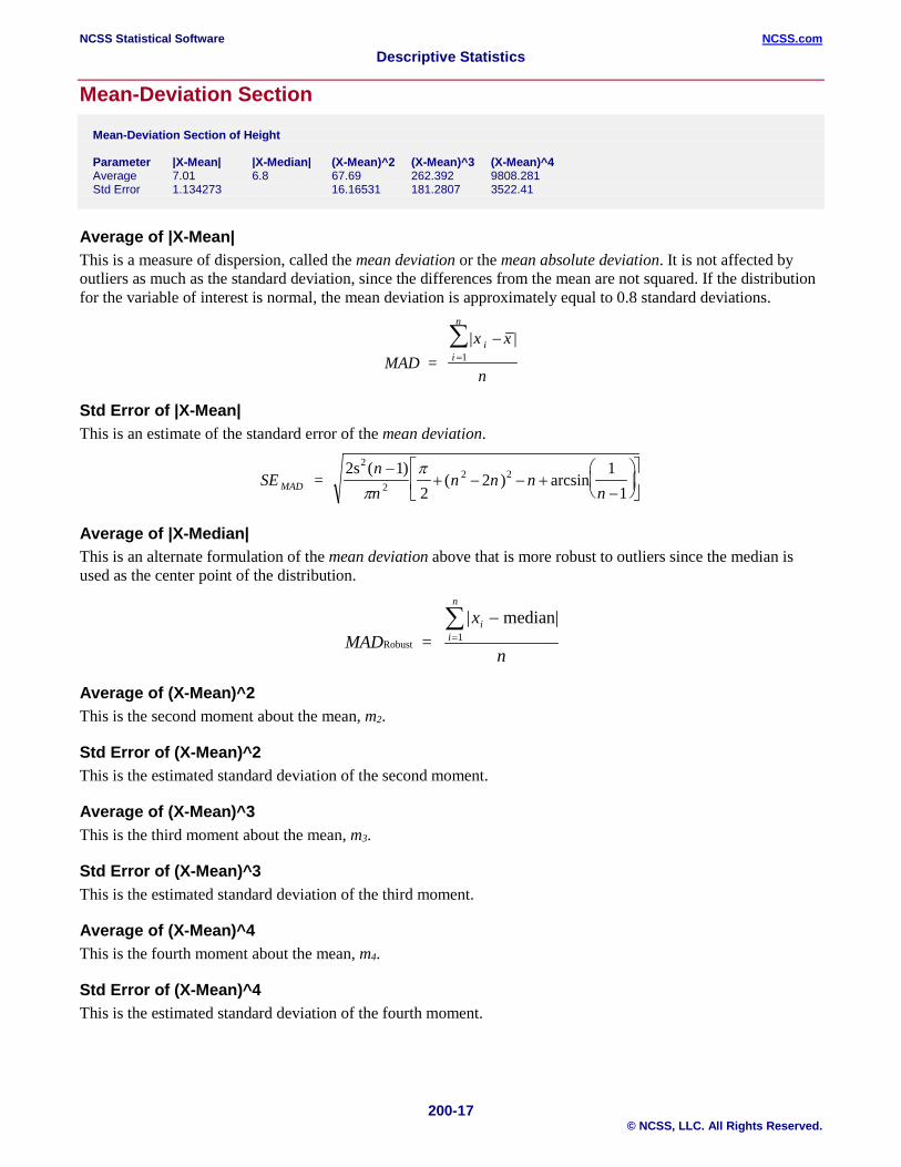
Mean-Deviation Section

Mean-Deviation Section of Height Parameter |X-Mean| |X-Median| (X-Mean)^2 (X-Mean)^3 (X-Mean)^4 Average 7.01 6.8 67.69 262.392 9808.281 Std Error 1.134273 16.16531 181.2807 3522.41

Average of |X-Mean| This is a measure of dispersion, called the mean deviation or the mean absolute deviation. It is not affected by outliers as much as the standard deviation, since the differences from the mean are not squared. If the distribution for the variable of interest is normal, the mean deviation is approximately equal to 0.8 standard deviations.

MADx x

n

ii

n

= ||

=∑ −

1

Std Error of |X-Mean| This is an estimate of the standard error of the mean deviation.

SEnn

n n nnMAD =

2s2 ( )( ) arcsin

−+ − − +

−

12

21

122 2

ππ

Average of |X-Median| This is an alternate formulation of the mean deviation above that is more robust to outliers since the median is used as the center point of the distribution.

MADx

n

ii

n

Robust = | median|

=∑ −

1

Average of (X-Mean)^2 This is the second moment about the mean, m2.

Std Error of (X-Mean)^2 This is the estimated standard deviation of the second moment.

Average of (X-Mean)^3 This is the third moment about the mean, m3.

Std Error of (X-Mean)^3 This is the estimated standard deviation of the third moment.

Average of (X-Mean)^4 This is the fourth moment about the mean, m4.

Std Error of (X-Mean)^4 This is the estimated standard deviation of the fourth moment.




Quartile Section This gives the value of the jth percentile. Of course, the 25th percentile is called the first (lower) quartile, the 50th percentile is the median, and the 75th percentile is called the third (upper) quartile.

Quartile Section of Height 10th 25th 50th 75th 90th Parameter Percentile Percentile Percentile Percentile Percentile Value 52 56 59.5 70 75.7 95% LCL 51 56 60 95% UCL 59 67 76

Value These are the values of the specified percentiles. Note that the definition of a percentile depends on the type of percentile that was specified.

LCL and 95% UCL These give an exact, 100(1-α)% confidence interval for the population percentile. This confidence interval does not assume normality. Instead, it only assumes a random sample of n items from a continuous distribution. The interval is based on the equation:

1 1 1− = − + − − +α I r n r I n r rp p( , ) ( , )

Here Ip(a,b) is the integral of the incomplete beta function:

I n r rnk

p pqk

rk n k( , ) ( )− + =

−

=

−−∑1 1

0

1

and q=1-p and Ip(a,b) = 1- I1-p(b,a).

Normality Test Section

Normality Test Section of Height Test Prob 10% Critical 5% Critical Decision Test Name Value Level Value Value (5%) Shapiro-Wilk W 0.9373675 0.2137298 Can't reject normality Anderson-Darling 0.4433714 0.2862859 Can't reject normality Martinez-Iglewicz 1.025854 1.216194 1.357297 Can't reject normality Kolmogorov-Smirnov 0.1482353 0.176 0.192 Can't reject normality D'Agostino Skewness 1.036739 0.2998578 1.645 1.96 Can't reject normality D'Agostino Kurtosis -0.7855 0.432156 1.645 1.96 Can't reject normality D'Agostino Omnibus 1.6918 0.429161 4.605 5.991 Can't reject normality

Normality Tests This section displays the results of seven tests of the hypothesis that the data come from the normal distribution. The Shapiro-Wilk andAnderson-Darling tests are usually considered as the best. The Kolmogorov-Smirnov test is included because of its historical popularity, but is bettered in almost every way by the other tests.

Unfortunately, these tests have small statistical power (probability of detecting nonnormal data) unless the sample sizes are large, say over 100. Hence, if the decision is to reject, you can be reasonably certain that the data are not normal. However, if the decision is to accept, the situation is not as clear. If you have a sample size of 100 or more, you can reasonably assume that the actual distribution is closely approximated by the normal distribution. If your sample size is less than 100, all you know is that there was not enough evidence in your data to reject the normality assumption. In other words, the data might be nonnormal, you just could not prove it. In this case, you must rely on the graphics and past experience to justify the normality assumption.




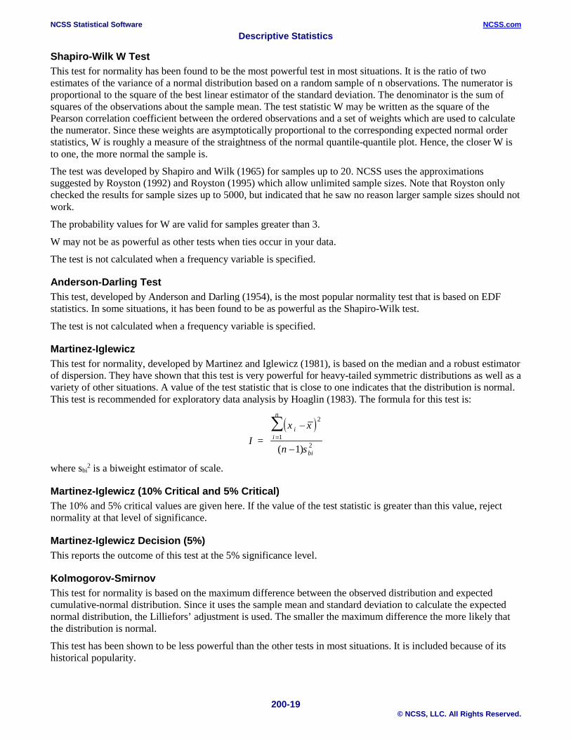
Shapiro-Wilk W Test This test for normality has been found to be the most powerful test in most situations. It is the ratio of two estimates of the variance of a normal distribution based on a random sample of n observations. The numerator is proportional to the square of the best linear estimator of the standard deviation. The denominator is the sum of squares of the observations about the sample mean. The test statistic W may be written as the square of the Pearson correlation coefficient between the ordered observations and a set of weights which are used to calculate the numerator. Since these weights are asymptotically proportional to the corresponding expected normal order statistics, W is roughly a measure of the straightness of the normal quantile-quantile plot. Hence, the closer W is to one, the more normal the sample is.

The test was developed by Shapiro and Wilk (1965) for samples up to 20. NCSS uses the approximations suggested by Royston (1992) and Royston (1995) which allow unlimited sample sizes. Note that Royston only checked the results for sample sizes up to 5000, but indicated that he saw no reason larger sample sizes should not work.

The probability values for W are valid for samples greater than 3.

W may not be as powerful as other tests when ties occur in your data.

The test is not calculated when a frequency variable is specified.

Anderson-Darling Test This test, developed by Anderson and Darling (1954), is the most popular normality test that is based on EDF statistics. In some situations, it has been found to be as powerful as the Shapiro-Wilk test.

The test is not calculated when a frequency variable is specified.

Martinez-Iglewicz This test for normality, developed by Martinez and Iglewicz (1981), is based on the median and a robust estimator of dispersion. They have shown that this test is very powerful for heavy-tailed symmetric distributions as well as a variety of other situations. A value of the test statistic that is close to one indicates that the distribution is normal. This test is recommended for exploratory data analysis by Hoaglin (1983). The formula for this test is:

( )I

x x

n s

ii

n

bi

= −

−=∑ 2

121( )

where sbi2 is a biweight estimator of scale.

Martinez-Iglewicz (10% Critical and 5% Critical) The 10% and 5% critical values are given here. If the value of the test statistic is greater than this value, reject normality at that level of significance.

Martinez-Iglewicz Decision (5%) This reports the outcome of this test at the 5% significance level.

Kolmogorov-Smirnov This test for normality is based on the maximum difference between the observed distribution and expected cumulative-normal distribution. Since it uses the sample mean and standard deviation to calculate the expected normal distribution, the Lilliefors’ adjustment is used. The smaller the maximum difference the more likely that the distribution is normal.

This test has been shown to be less powerful than the other tests in most situations. It is included because of its historical popularity.




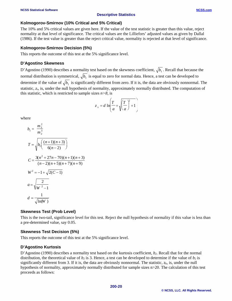
Kolmogorov-Smirnov (10% Critical and 5% Critical) The 10% and 5% critical values are given here. If the value of the test statistic is greater than this value, reject normality at that level of significance. The critical values are the Lilliefors’ adjusted values as given by Dallal (1986). If the test value is greater than the reject critical value, normality is rejected at that level of significance.

Kolmogorov-Smirnov Decision (5%) This reports the outcome of this test at the 5% significance level.

D’Agostino Skewness D’Agostino (1990) describes a normality test based on the skewness coefficient, b1 . Recall that because the normal distribution is symmetrical, b1 is equal to zero for normal data. Hence, a test can be developed to determine if the value of b1 is significantly different from zero. If it is, the data are obviously nonnormal. The statistic, zs, is, under the null hypothesis of normality, approximately normally distributed. The computation of this statistic, which is restricted to sample sizes n>8, is

z dTa

Tas = +

+

ln

2

1

where

bmm1 = 3

2

23

T b n nn

=+ +

−

1

1 36 2

( )( )( )

C n n n nn n n n

=+ − + +− + + +

3 27 70 1 32 5)( 7 9

2( )( )( )( )( )( )

W C2 1 2 1= − + −( )

aW

=−

212

dW

=1

ln( )

Skewness Test (Prob Level) This is the two-tail, significance level for this test. Reject the null hypothesis of normality if this value is less than a pre-determined value, say 0.05.

Skewness Test Decision (5%) This reports the outcome of this test at the 5% significance level.

D’Agostino Kurtosis D’Agostino (1990) describes a normality test based on the kurtosis coefficient, b2. Recall that for the normal distribution, the theoretical value of b2 is 3. Hence, a test can be developed to determine if the value of b2 is significantly different from 3. If it is, the data are obviously nonnormal. The statistic, zk, is, under the null hypothesis of normality, approximately normally distributed for sample sizes n>20. The calculation of this test proceeds as follows:




z

AA

GA

A

k =

−

−

−

+−

12

9

12

12

42

9

1 3/

where

bmm2 = 4

22

Gb n

nn n n

n n n

=−

−+

− −+ + +

2

2

3 31

24 2 31 3 5)

( )( )( ) ( )(

E n nn n

n nn n n

=− +

+ ++ +− −

6 5 27 9

6 3 5)2 3

2( )( )( )

( )(( )( )

AE E E

= + + +

6 8 2 1 4

2

Prob Level of Kurtosis Test This is the two-tail significance level for this test. Reject the null hypothesis of normality if this value is less than a pre-determined value, say 0.05.

Decision of Kurtosis Test This reports the outcome of this test at the 5% significance level.

D’Agostino Omnibus D’Agostino (1990) describes a normality test that combines the tests for skewness and kurtosis. The statistic, K2, is approximately distributed as a chi-square with two degrees of freedom. After calculated zs and zk, calculate K2 as follows:

K z zs k2 2 2= +

Prob Level D’Agostino Omnibus This is the significance level for this test. Reject the null hypothesis of normality if this value is less than a pre-determined value, say 0.05.

Decision of D’Agostino Omnibus Test This reports the outcome of this test at the 5% significance level.




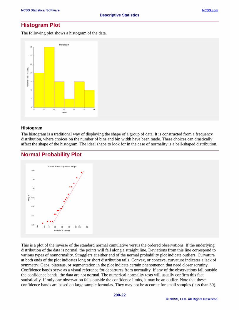
Histogram Plot The following plot shows a histogram of the data.

Histogram The histogram is a traditional way of displaying the shape of a group of data. It is constructed from a frequency distribution, where choices on the number of bins and bin width have been made. These choices can drastically affect the shape of the histogram. The ideal shape to look for in the case of normality is a bell-shaped distribution.

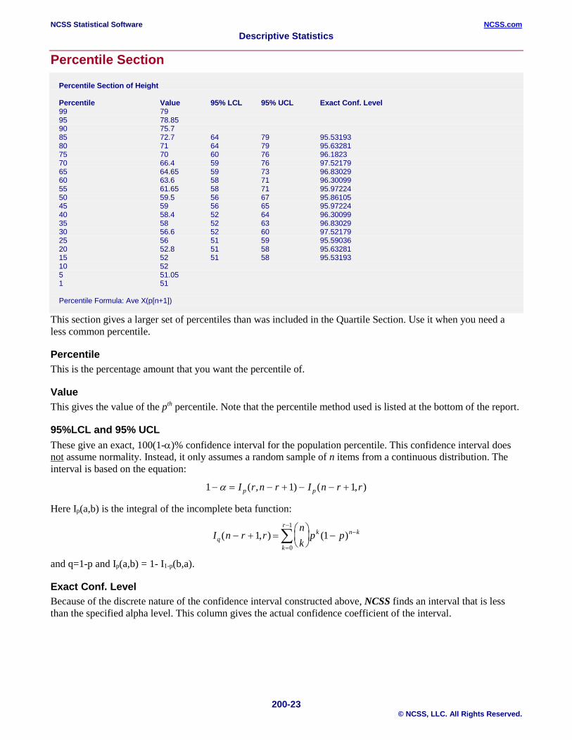
Normal Probability Plot

This is a plot of the inverse of the standard normal cumulative versus the ordered observations. If the underlying distribution of the data is normal, the points will fall along a straight line. Deviations from this line correspond to various types of nonnormality. Stragglers at either end of the normal probability plot indicate outliers. Curvature at both ends of the plot indicates long or short distribution tails. Convex, or concave, curvature indicates a lack of symmetry. Gaps, plateaus, or segmentation in the plot indicate certain phenomenon that need closer scrutiny. Confidence bands serve as a visual reference for departures from normality. If any of the observations fall outside the confidence bands, the data are not normal. The numerical normality tests will usually confirm this fact statistically. If only one observation falls outside the confidence limits, it may be an outlier. Note that these confidence bands are based on large sample formulas. They may not be accurate for small samples (less than 30).




Percentile Section Percentile Section of Height Percentile Value 95% LCL 95% UCL Exact Conf. Level 99 79 95 78.85 90 75.7 85 72.7 64 79 95.53193 80 71 64 79 95.63281 75 70 60 76 96.1823 70 66.4 59 76 97.52179 65 64.65 59 73 96.83029 60 63.6 58 71 96.30099 55 61.65 58 71 95.97224 50 59.5 56 67 95.86105 45 59 56 65 95.97224 40 58.4 52 64 96.30099 35 58 52 63 96.83029 30 56.6 52 60 97.52179 25 56 51 59 95.59036 20 52.8 51 58 95.63281 15 52 51 58 95.53193 10 52 5 51.05 1 51 Percentile Formula: Ave X(p[n+1]) This section gives a larger set of percentiles than was included in the Quartile Section. Use it when you need a less common percentile.

Percentile This is the percentage amount that you want the percentile of.

Value This gives the value of the pth percentile. Note that the percentile method used is listed at the bottom of the report.

95%LCL and 95% UCL These give an exact, 100(1-α)% confidence interval for the population percentile. This confidence interval does not assume normality. Instead, it only assumes a random sample of n items from a continuous distribution. The interval is based on the equation:

1 1 1− = − + − − +α I r n r I n r rp p( , ) ( , )

Here Ip(a,b) is the integral of the incomplete beta function:

I n r rnk

p pqk

rk n k( , ) ( )− + =

−

=

−−∑1 1

0

1

and q=1-p and Ip(a,b) = 1- I1-p(b,a).

Exact Conf. Level Because of the discrete nature of the confidence interval constructed above, NCSS finds an interval that is less than the specified alpha level. This column gives the actual confidence coefficient of the interval.




Stem-and-Leaf Plot Section Stem-and-Leaf Plot Section of Height Depth Stem Leaves 4 5* | 1222 10 . | 668899 10 6* | 034 7 . | 57 5 7* | 113 2 . | 69 Unit = 1 Example: 1|2 Represents 12 The stem-leaf plot is a type of histogram which retains much of the identity of the original data. It is useful for finding data-entry errors as well as for studying the distribution of a variable.

Depth This is the cumulative number of leaves, counting in from the nearest end.

Stem The stem is the first digit of the actual number. For example, the stem of the number 523 is 5 and the stem of 0.0325 is 3. This is modified appropriately if the batch contains numbers of different orders of magnitude. The largest order of magnitude is used in determining the stem. Depending upon the number of leaves, a stem may be divided into two or more sub-stems. A special set of symbols is then used to mark the stems.

The star (*) represents numbers in the range of zero to four, while the period (.) represents numbers in the range of five to nine.

Leaf The leaf is the second digit of the actual number. For example, the leaf of the number 523 is 2 and the leaf of 0.0325 is 2. This is modified appropriately if the batch contains numbers of different orders of magnitude. The largest order of magnitude is used in determining the leaf.

Unit This line at the bottom indicates how the data were scaled to make the plot.


Documents

Chapter 200 Descriptive Statistics - · PDF fileChapter 200 Descriptive Statistics Introduction This procedure summarizes variables both statistically and graphically. ... A kurtosis