Embed Size (px)
Citation preview

© Goodwin, Graebe, Salgado , Prentice Hall 2000Chapter 26
Chapter 26
DecouplingDecoupling

© Goodwin, Graebe, Salgado , Prentice Hall 2000Chapter 26
An idealized requirement in MIMO control-system designis that of decoupling. If a plant is dynamically decoupled,then changes in the set-point of one process variable leadto a response in that process variable but all other processvariables remain constant. The advantages of such adesign are intuitively clear: e.g., a temperature may berequired to be changed, but it may be undesirable forother variables (e.g., pressure) to suffer any associatedtransient. Full dynamic decoupling is a very stringentrequirement. Thus, in practice, it is more usual to seekdynamic decoupling over some desired bandwidth.

© Goodwin, Graebe, Salgado , Prentice Hall 2000Chapter 26
This chapter describes the design proceduresnecessary to achieve dynamic decoupling. Inparticular, we discuss
dynamic decoupling for stable minimum-phase systems
dynamic decoupling for stable nonminimum-phasesystems
dynamic decoupling for open-loop unstable systems

© Goodwin, Graebe, Salgado , Prentice Hall 2000Chapter 26
As might be expected, full dynamic decoupling is astrong requirement and is generally not cost-free.We will thus also quantify the performance cost ofdecoupling by using frequency-domain procedures.These allow a designer to assess a-priori whether thecost associated with decoupling is acceptable in agiven application.

© Goodwin, Graebe, Salgado , Prentice Hall 2000Chapter 26
Of course, some form of decoupling is a very commonrequirement. For example, static decoupling is almostalways a design requirement. The question thenbecomes, over what bandwidth will decoupling(approximately) be asked for? It will turn out that theadditional cost of decoupling is a function of open-loop poles and zeros in the right-half plane. Thus ifone is restricting decoupling in some bandwidth, thenby focusing attention on those open-loop poles andzeros that fall within this bandwidth, one can get a feelfor the cost of decoupling over that bandwidth.

© Goodwin, Graebe, Salgado , Prentice Hall 2000Chapter 26
We will also examine the impact of actuatorsaturation on decoupling. In the case of staticdecoupling, it is necessary to avoid integrator wind-up. This can be achieved by using methods that areanalogous to the SISO case treated in Chapter 11.

© Goodwin, Graebe, Salgado , Prentice Hall 2000Chapter 26
Stable Systems
We first consider the situation in which the open-looppoles of the plant are located in desirable locations.We will employ the affine-parameterizationtechnique described in Chapter 25 to design acontroller that achieves full dynamic decoupling.

© Goodwin, Graebe, Salgado , Prentice Hall 2000Chapter 26
Stable Systems:Part 1 - Minimum-Phase CaseWe refer to the general Q-design procedure outlined inChapter 25.To achieve dynamic decoupling, we make the followingchoice for Q(s).
Where ξξξξR(s) is the right interactor, and p1(s), p2(s), …pm(s) are stable polynomials chosen to make Q(s) proper.The polynomials p1(s), p2(s), … pm(s) should be chosento have unit d.c. gain.
Q(s) = ξR(s)[ΛR(s)]−1DQ(s)ΛR(s) = Go(s)ξR(s)
DQ(s) = diag(
1p1(s)
,1
p2(s), · · · , 1
pm(s)
)

© Goodwin, Graebe, Salgado , Prentice Hall 2000Chapter 26
We observe that, with the above choice, we achievethe following nominal complementary sensitivity:
To(s) = Go(s)Q(s)
= Go(s)ξR(s)[ΛR(s)]−1DQ(s)
= Go(s)ξR(s)[Go(s)ξR(s)]−1DQ(s)
= diag(
1p1(s)
,1
p2(s), · · · , 1
pm(s)
)

© Goodwin, Graebe, Salgado , Prentice Hall 2000Chapter 26
We see that this is diagonal, as required. Theassociated control-system structure would then be asshown below:
Figure 26.1: IMC decoupled control of stable MIMOplants
Plant
Go(s)
R(s)y(t)u(t)u(t)
[ΛR(s)]−1u(t)DQ(s)
ν(t)
−+
−
+
.

© Goodwin, Graebe, Salgado , Prentice Hall 2000Chapter 26
Actually, the above design is not unique. Forexample, an alternative choice for Q(s) is
where DQ(s) is given by
=)(
1,,)(
1,)(
1)(21 spspsp
diagsm
QD
Q(s) = [ΛL(s)]−1ξL(s)DQ(s)

© Goodwin, Graebe, Salgado , Prentice Hall 2000Chapter 26
Note also that DQ(s) can have the more generalstructure
where t1(s), t2(s), …, tm(s) are proper stable transferfunctions having relative degrees equal to thecorresponding column degrees of the left interactorfor Go(s). The transfer functions t1(s), t2(s), …, tm(s)should be chosen to have unit d.c. gain.
DQ(s) = diag (t1(s), t2(s), · · · , tm(s))

© Goodwin, Graebe, Salgado , Prentice Hall 2000Chapter 26
Example 26.1
Consider a stable 2 × 2 MIMO system having thenominal model
Choose a suitable matrix Q(s) to control this plant,using the affine parameterization, in such a way thatthe MIMO control loop is able to track references ofbandwidths less than or equal to 2[rad/s] and 4[rad/s]in channels 1 and 2, respectively.
Go(s) =1
(s+ 1)2(s+ 2)
[2(s+ 1) −1(s+ 1)2 (s+ 1)(s+ 2)
]

© Goodwin, Graebe, Salgado , Prentice Hall 2000Chapter 26
We will aim to obtain a complementary sensitivitymatrix given by
where T11(s) and T22(s) will be chosen to havebandwidths 2[rad/s] and 4[rad/s] in channels 1 and 2,respectively.
To(s) = diag(T11(s), T22(s))
© Goodwin, Graebe, Salgado , Prentice Hall 2000Chapter 26
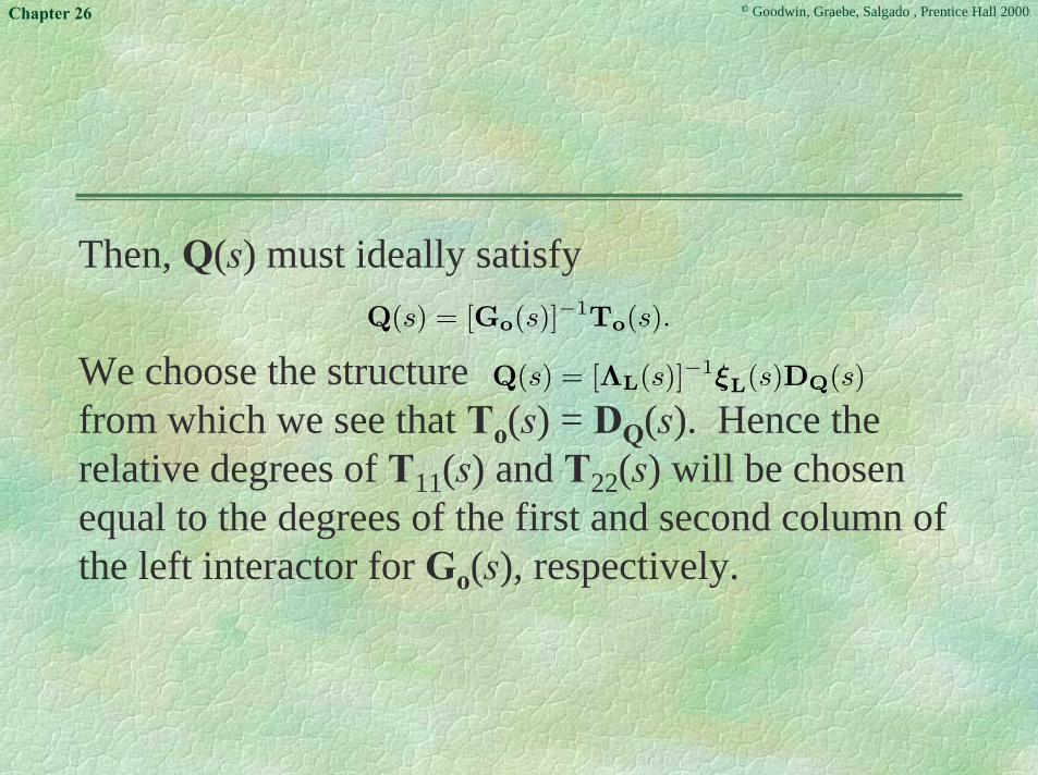
Then, Q(s) must ideally satisfy
We choose the structurefrom which we see that To(s) = DQ(s). Hence therelative degrees of T11(s) and T22(s) will be chosenequal to the degrees of the first and second column ofthe left interactor for Go(s), respectively.
Q(s) = [Go(s)]−1To(s).
Q(s) = [ΛL(s)]−1ξL(s)DQ(s)
© Goodwin, Graebe, Salgado , Prentice Hall 2000Chapter 26
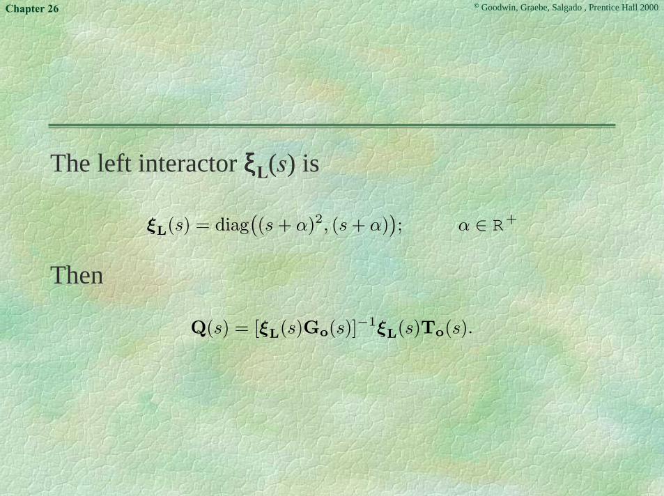
The left interactor ξξξξL(s) is
Then
ξL(s) = diag((s+ α)2, (s+ α)
); α ∈ R+
Q(s) = [ξL(s)Go(s)]−1ξL(s)To(s).

© Goodwin, Graebe, Salgado , Prentice Hall 2000Chapter 26
Hence, Q(s) is proper if and only if To(s) is chosen soas to make ξξξξL(s)To(s) proper.
Thus, possible choices for T11(s) and T22(s) are
T11(s) =4
s2 + 3s+ 4; and T22(s) =
4(s+ 4)s2 + 6s+ 16

© Goodwin, Graebe, Salgado , Prentice Hall 2000Chapter 26
To obtain the final expression for Q(s), we next needto compute [Go(s)]-1, which is given by
[Go(s)]−1 =s+ 22s+ 5
[(s+ 1)(s+ 2) 1−(s+ 1)2 2(s+ 1)
]
© Goodwin, Graebe, Salgado , Prentice Hall 2000Chapter 26
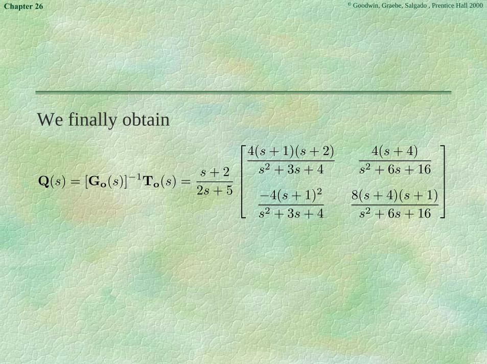
We finally obtain
Q(s) = [Go(s)]−1To(s) =s+ 22s+ 5
4(s+ 1)(s+ 2)s2 + 3s+ 4
4(s+ 4)s2 + 6s+ 16
−4(s+ 1)2s2 + 3s+ 4
8(s+ 4)(s+ 1)s2 + 6s+ 16

© Goodwin, Graebe, Salgado , Prentice Hall 2000Chapter 26
The above design procedure is limited to minimum-phase systems. In particular, it is clear that Q(s),chosen as above, is stable if and only if Go(s) isminimum phase, because [ΛΛΛΛR(s)]-1 and [ΛΛΛΛL(s)]-1
involve an inverse of Go(s). We therefore need tomodify Q(s) so as to ensure stability when Go(s) isnonminimum phase. A way of doing this isdescribed below.

© Goodwin, Graebe, Salgado , Prentice Hall 2000Chapter 26
Stable Systems:Part 2 - Nonminimum-Phase Case
We will begin with the state space realization for[ΛΛΛΛR(s)]-1, defined by a 4-tuple (Aλ, Bλ, Cλ, Dλ). Wewill denote by ũ(t) the input to this system. Our aimis to modify [ΛΛΛΛR(s)]-1 so as to achieve two objectives:
(i) render the transfer function stable, whilst;(ii) retaining its diagonalizing properties.

© Goodwin, Graebe, Salgado , Prentice Hall 2000Chapter 26
To this end, we define the following subsystem,which is driven by the ith component of ũ(t)
where υi(t) ∈ m, ũi(t) ∈ , and (Ai, Bi, Ci, Di) is aminimal realization of the transfer function from theith component of ũ(t) to the complete vector outputū(t). Thus (Ai, Bi, Ci, Di) is a minimal realization of(Aλ, Bλei, Cλ, Dλei), where ei is the ith column of them × m identity matrix.
xi(t) = Aixi(t) +Biui(t)υi(t) = Cixi(t) +Diui(t)

© Goodwin, Graebe, Salgado , Prentice Hall 2000Chapter 26
We next apply stabilizing state feedback to each ofthese subsystems - i.e., we form
where ∈ . The design of Ki can be done inany convenient fashion - e.g., by linear quadraticoptimization.
)( tri
ui(t) = −Kixi(t) + ri(t); i = 1, 2, . . . ,m

© Goodwin, Graebe, Salgado , Prentice Hall 2000Chapter 26
Finally we add together the m vectors υ1(t), υ2(t), …υm(t) to produce an output, which can be renamedū(t):
We then have the following result:
u(t) =m∑
i=1
υi(t)
© Goodwin, Graebe, Salgado , Prentice Hall 2000Chapter 26
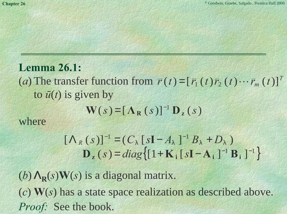
Lemma 26.1:(a) The transfer function from
to ū(t) is given by
where
(b)ΛΛΛΛR(s)W(s) is a diagonal matrix.(c) W(s) has a state space realization as described above.Proof: See the book.
Tm trtrtrtr )]()()([)( 21 =
)()]([)( 1 sss zR DΛW −=
11
11
]][1[)()][()]([
−−λλ
−λλ
−
−+=+−=Λ
iiiz BAIKDI
sdiagsDBAsCsR

© Goodwin, Graebe, Salgado , Prentice Hall 2000Chapter 26
Returning now to the problem of determining Q(s),we choose
This is equivalent to
Then
Q(s) = ξR(s)W(s)DQ(s)
Q(s) = ξR(s)[ξR(s)]−1[Go(s)]−1Dz(s)DQ(s)
Q(s) = [Go(s)]−1Dz(s) diag t1(s), t2(s), · · · , tm(s)
© Goodwin, Graebe, Salgado , Prentice Hall 2000Chapter 26
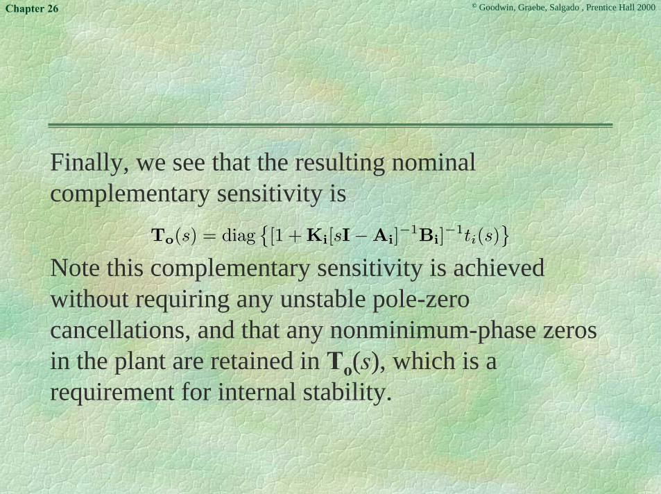
Finally, we see that the resulting nominalcomplementary sensitivity is
Note this complementary sensitivity is achievedwithout requiring any unstable pole-zerocancellations, and that any nonminimum-phase zerosin the plant are retained in To(s), which is arequirement for internal stability.
To(s) = diag[1 +Ki[sI− Ai]−1Bi]−1ti(s)
© Goodwin, Graebe, Salgado , Prentice Hall 2000Chapter 26
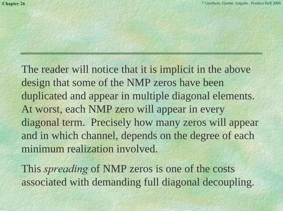
The reader will notice that it is implicit in the abovedesign that some of the NMP zeros have beenduplicated and appear in multiple diagonal elements.At worst, each NMP zero will appear in everydiagonal term. Precisely how many zeros will appearand in which channel, depends on the degree of eachminimum realization involved.
This spreading of NMP zeros is one of the costsassociated with demanding full diagonal decoupling.

© Goodwin, Graebe, Salgado , Prentice Hall 2000Chapter 26
Decoupling Invariants
Actually, the NMP zeros appearing in
are diagonalizing invariants and appear in all possiblediagonalized closed loops. Thus, spreading NMPdynamics into other channels is a trade-off inherentlyassociated with decoupling.
The final implementation of Q(s) is as shown below.
To(s) = diag[1 +Ki[sI− Ai]−1Bi]−1ti(s)

© Goodwin, Graebe, Salgado , Prentice Hall 2000Chapter 26
Figure 26.2: Diagonal decoupling MIMO controller(Q(s))
K1
υ1(t)S1
υm(t)
r1R
rm
r r2u(t)υ2(t)ν(t)
+
x1(t)
+
−
diag ti(s)u(t)
© Goodwin, Graebe, Salgado , Prentice Hall 2000Chapter 26
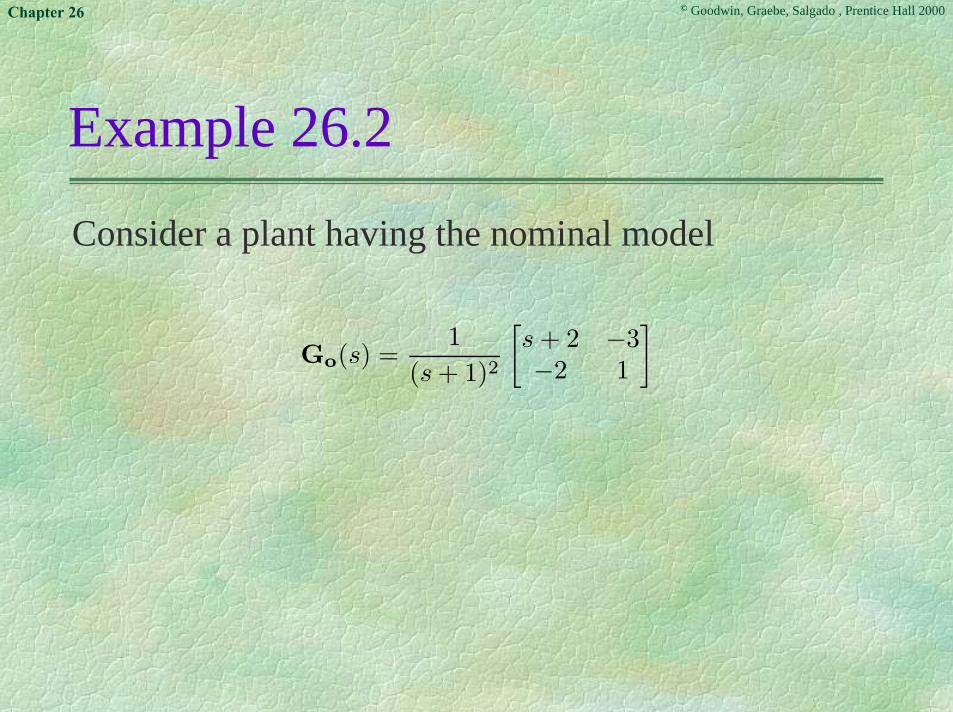
Example 26.2
Consider a plant having the nominal model
Go(s) =1
(s+ 1)2
[s+ 2 −3−2 1
]

© Goodwin, Graebe, Salgado , Prentice Hall 2000Chapter 26
This model has a NMP zero at s = 4. To synthesize acontroller following the ideas presented above, we firstcompute a right interactor matrix, which turns out tohave the general form ξξξξR(s) = diags + α, (s + α)2.For numerical simplicity, we choose α = 1. Then
and a state space realization for [ΛΛΛΛR(s)]-1 is
[ΛR(s)]−1 = [Go(s)ξR(s)]−1 =
1s− 4
[s+ 1 3(s+ 1)2 s+ 2
]
A =[4 00 4
]; B = I ; C =
[5 152 6
]; D =
[1 30 1
]
© Goodwin, Graebe, Salgado , Prentice Hall 2000Chapter 26
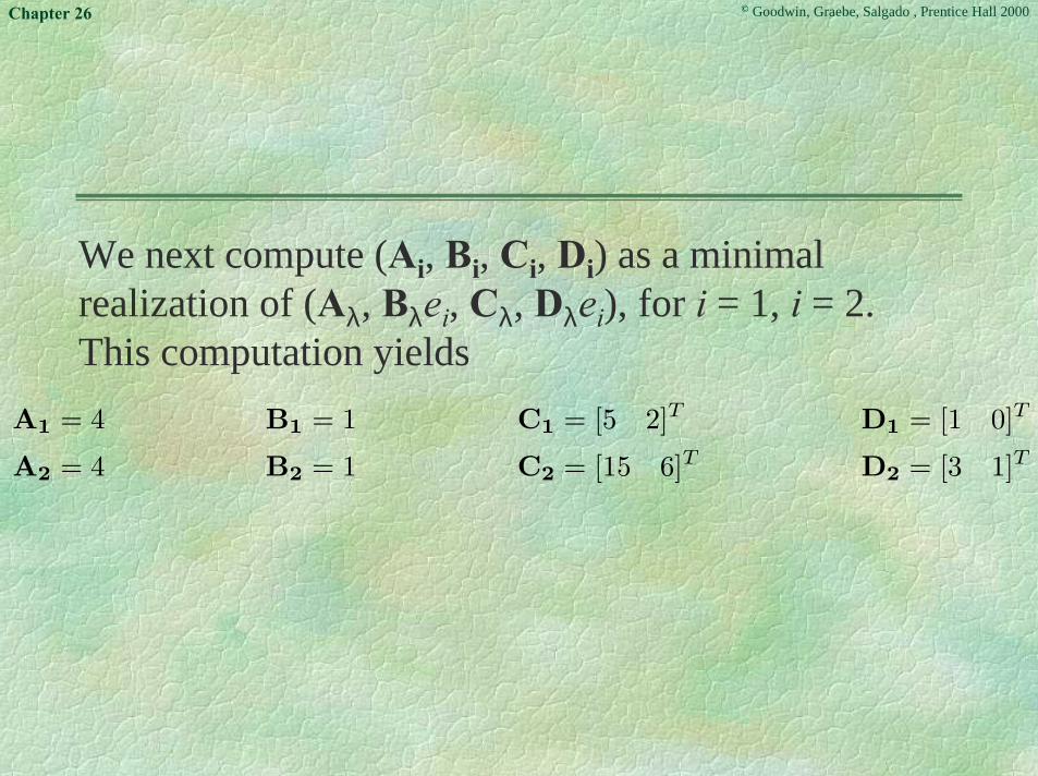
We next compute (Ai, Bi, Ci, Di) as a minimalrealization of (Aλ, Bλei, Cλ, Dλei), for i = 1, i = 2.This computation yields
A1 = 4 B1 = 1 C1 = [5 2]T D1 = [1 0]T
A2 = 4 B2 = 1 C2 = [15 6]T D2 = [3 1]T

© Goodwin, Graebe, Salgado , Prentice Hall 2000Chapter 26
These subsystems can be stabilized by state feedbackwith gains K1 and K2, respectively. For this case,each gain is chosen to shift the unstable pole at s = 4to a stable location, say s = -10, which leads to K1 =K2 = 14. Thus, Dz(s) is a 2 × 2 diagonal matrix givenby
Dz(s) =s− 4s+ 10
I

© Goodwin, Graebe, Salgado , Prentice Hall 2000Chapter 26
We finally choose DQ(s) to achieve a bandwidthapproximately equal to 3[rad/s], say
DQ(s) = diag
−9(s+ 10)4(s2 + 4s+ 9)
−904(s2 + 4s+ 9)
© Goodwin, Graebe, Salgado , Prentice Hall 2000Chapter 26
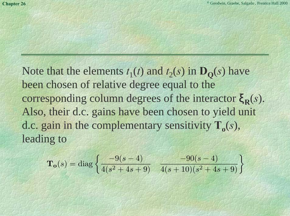
Note that the elements t1(t) and t2(s) in DQ(s) havebeen chosen of relative degree equal to thecorresponding column degrees of the interactor ξξξξR(s).Also, their d.c. gains have been chosen to yield unitd.c. gain in the complementary sensitivity To(s),leading to
To(s) = diag
−9(s− 4)4(s2 + 4s+ 9)
−90(s− 4)4(s+ 10)(s2 + 4s+ 9)

© Goodwin, Graebe, Salgado , Prentice Hall 2000Chapter 26
Pre- and PostDiagonalization
The transfer-function matrix Q(s) presented in
is actually a right-diagonalizing compensator for astable (but not necessarily minimum-phase) plant.This can be seen by noting that
where
Q(s) = ξR(s)W(s)DQ(s)
Go(s)ΠR(s) = diag[1 +Ki[sI− Ai]−1Bi]−1ti(s)
ΠR(s) = Q(s)= ξR(s)W(s)DQ(s)
© Goodwin, Graebe, Salgado , Prentice Hall 2000Chapter 26
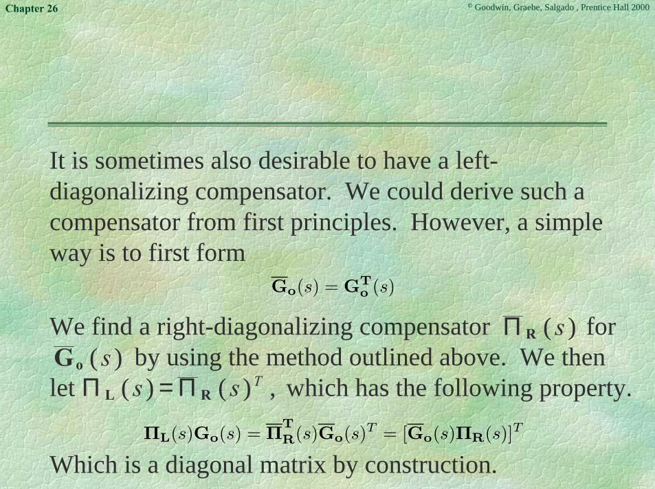
It is sometimes also desirable to have a left-diagonalizing compensator. We could derive such acompensator from first principles. However, a simpleway is to first form
We find a right-diagonalizing compensator for by using the method outlined above. We then
let which has the following property.
Which is a diagonal matrix by construction.
)( sRΠ)( soG
,)()( Tss RL Π=Π
ΠL(s)Go(s) = ΠT
R(s)Go(s)T = [Go(s)ΠR(s)]T
Go(s) = GTo (s)

© Goodwin, Graebe, Salgado , Prentice Hall 2000Chapter 26
Unstable Systems
We next turn to the problem of designing adecoupling controller for an unstable MIMO plant.Here we have an additional complexity: someminimal feedback is necessary to ensure stability. Togain insight into this problem, we describe fouralternative design choices in the book; namely

© Goodwin, Graebe, Salgado , Prentice Hall 2000Chapter 26
(i) a two-degree-of-freedom design based onprefiltering the reference;
(ii) a two-degree-of-freedom design using the affineparameterization;
(iii) a design based on one-degree-of-freedom statefeedback; and
(iv) a design integrating both state feedback and theaffine parameterization.

© Goodwin, Graebe, Salgado , Prentice Hall 2000Chapter 26
Two-Degree-of-Freedom DesignBased on PreFiltering the Reference
If one requires full dynamic decoupling forreference-signal changes only, then this can bereadily achieved by first stabilizing the system byusing some suitable controller C(s) and then usingprefiltering of the reference signal. The essential ideais illustrated on the next slide.

© Goodwin, Graebe, Salgado , Prentice Hall 2000Chapter 26
Figure 26.3: Prefilter design for full dynamic decoupling
r(t)H(s) C(s)
+
−Plant
Prefilter
y(t)
© Goodwin, Graebe, Salgado , Prentice Hall 2000Chapter 26
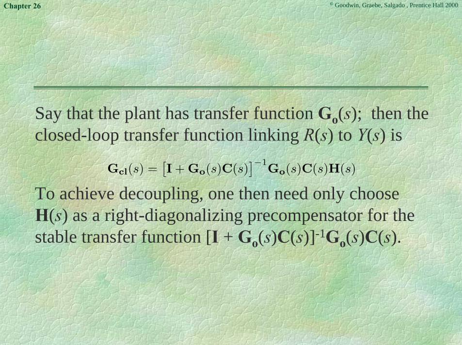
Say that the plant has transfer function Go(s); then theclosed-loop transfer function linking R(s) to Y(s) is
To achieve decoupling, one then need only chooseH(s) as a right-diagonalizing precompensator for thestable transfer function [I + Go(s)C(s)]-1Go(s)C(s).
Gcl(s) =[I+Go(s)C(s)
]−1Go(s)C(s)H(s)

© Goodwin, Graebe, Salgado , Prentice Hall 2000Chapter 26
Example 26.4
Consider the plant
whereGo(s) = GoN(s)[GoD(s)]−1
GoN(s) =[−5 s2
1 −0.0023
]; GoD(s) =
[25s+ 1 00 s(s+ 1)2
]
© Goodwin, Graebe, Salgado , Prentice Hall 2000Chapter 26
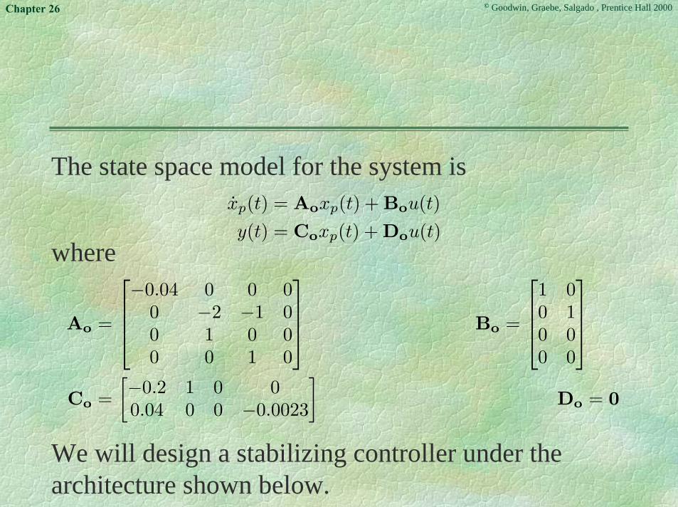
The state space model for the system is
where
We will design a stabilizing controller under thearchitecture shown below.
xp(t) = Aoxp(t) +Bou(t)y(t) = Coxp(t) +Dou(t)
Ao =
−0.04 0 0 00 −2 −1 00 1 0 00 0 1 0
Bo =
1 00 10 00 0
Co =[−0.2 1 0 00.04 0 0 −0.0023
]Do = 0

© Goodwin, Graebe, Salgado , Prentice Hall 2000Chapter 26
Figure 26.4: Optimal quadratic design with integralaction
Plant
Observer
−
−
+
z(t)
y(t)
− e(t)
xp(t)
K1
K2
u(t)
r(t)dg(t)
1s
I

© Goodwin, Graebe, Salgado , Prentice Hall 2000Chapter 26
We design an observer for the state xp(t), given theoutput y(t). This design uses Kalman-filter theorywith Q = BoBo
T and R = 0.05I2×2.The optimal observer gains turn out to be
J =
−3.9272 1.36442.6120 0.1221−0.6379 0.1368−2.7266 −4.6461

© Goodwin, Graebe, Salgado , Prentice Hall 2000Chapter 26
We wish to have zero steady-state errors in the faceof step input disturbances. We therefore introduce anintegrator with transfer function I/s at the output ofthe system (after the comparator). That is, we add
z(t) = −y(t) = −Coxp(t)

© Goodwin, Graebe, Salgado , Prentice Hall 2000Chapter 26
We can now define a composite state vector leading to the composite model
where
TTTp tztxtx )]()([)( =
x(t) = Ax(t) +Bu(t)
A =[
Ao 0−Co 0
]; B =
[Bo
0
]

© Goodwin, Graebe, Salgado , Prentice Hall 2000Chapter 26
We next consider the composite system and design astate variable feedback controller via LQR theory.
We choose
Ψ =
Co
TCo 0 00 0.005 00 0 0.1
; Φ = 2I2×2

© Goodwin, Graebe, Salgado , Prentice Hall 2000Chapter 26
Leading to the feedback gain K = [K1 K2], where
K1 =[0.1807 −0.0177 0.1011 −0.0016−0.0177 0.1496 0.0877 0.0294
]; K2 =
[0.0412 −0.12640.0283 0.1844
]
© Goodwin, Graebe, Salgado , Prentice Hall 2000Chapter 26
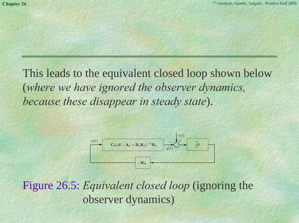
This leads to the equivalent closed loop shown below(where we have ignored the observer dynamics,because these disappear in steady state).
Figure 26.5: Equivalent closed loop (ignoring the observer dynamics)
u(t) +−y(t)
1
sI
−K2
r(t)
Co(sI− Ao + BoK1)−1Bo

© Goodwin, Graebe, Salgado , Prentice Hall 2000Chapter 26
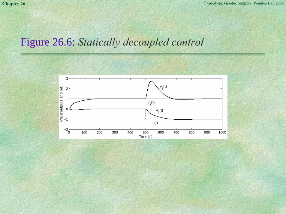
The resulting closed-loop responses for unit stepreferences are shown on the next slide where r1(t) =µ(t - 1) and r2(t) = -µ(t - 501). Note that, as expected,the system is statically decoupled, but significantdynamic coupling occurs during transients, especiallyfollowing the step in the second reference.
© Goodwin, Graebe, Salgado , Prentice Hall 2000Chapter 26
Figure 26.6: Statically decoupled control
0 100 200 300 400 500 600 700 800 900 1000−2
−1
0
1
2
3
Time [s]
Pla
nt o
utpu
ts a
nd r
ef. y
1(t)
r1(t)
y2(t)
r2(t)
© Goodwin, Graebe, Salgado , Prentice Hall 2000Chapter 26
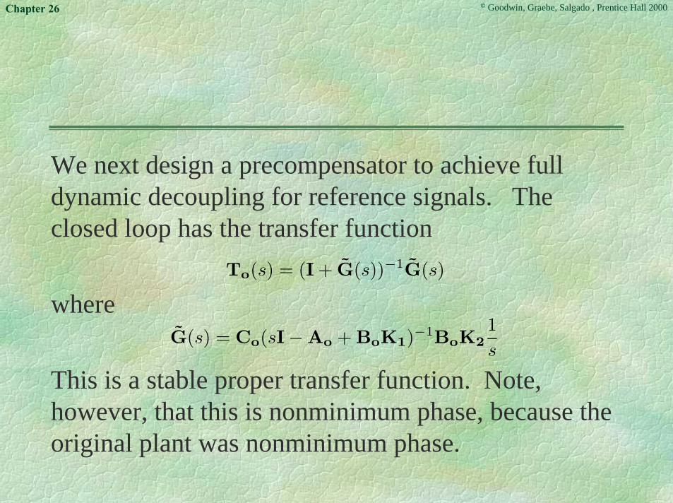
We next design a precompensator to achieve fulldynamic decoupling for reference signals. Theclosed loop has the transfer function
where
This is a stable proper transfer function. Note,however, that this is nonminimum phase, because theoriginal plant was nonminimum phase.
To(s) = (I+ G(s))−1G(s)
G(s) = Co(sI− Ao +BoK1)−1BoK21s

© Goodwin, Graebe, Salgado , Prentice Hall 2000Chapter 26
We use the techniques outlined above to design aright inverse that retains dynamic decoupling in thepresence of nonminimum-phase zeros. To use thosetechniques, the equivalent plant is the closed-loopsystem with transfer functionand with state space model given by the 4-tuple (Ae,Be, Ce, 0), where
To(s) = (I+ G(s))−1G(s)
Ae =[Ao − BoK1 BoK2
−Co 0
]; Be =
[0 I
]T ; Ce =[Co 0
]

© Goodwin, Graebe, Salgado , Prentice Hall 2000Chapter 26
A suitable interactor for this closed-loop system is
03.0;)(0
0)()( 2
2
=
++= α
ααξ
sssL

© Goodwin, Graebe, Salgado , Prentice Hall 2000Chapter 26
This leads to an augmented system having the statespace model with( )eeee D,CBA ′′′′ ,,
eeee
eeeeee
ee
ee
BACDACACCC
BBAA
=′++=′
=′=′
22 2αα

© Goodwin, Graebe, Salgado , Prentice Hall 2000Chapter 26
The exact inverse then has the state space model(Aλ, Bλ, Cλ, Dλ), where
1
1
1
1
][][
][][
−
−
−
−
′=′′=′′′=
′′′−′=
e
ee
eee
eeee
DDCD-C
CDBBCDBAA
λ
λ
λ
λ

© Goodwin, Graebe, Salgado , Prentice Hall 2000Chapter 26
We now form the two subsystems as describedearlier. We form minimal realizations of these twosystems, which we denote by (A1, B1, C1, D1) and(A2, B2, C2, D2) . We determine stabilizing feedbackfor these two systems by using LQR theory with
722
61111
1010====22222222 ΦΦΦΦΨΨΨΨ
ΦΦΦΦΨΨΨΨCCCC
T
T

© Goodwin, Graebe, Salgado , Prentice Hall 2000Chapter 26
We then implement the precompensator as in Figure26.2, where we choose
where K1, K2 now represent the stabilizing gains forthe two subsystems.
22
1222
2
21
1112
1
)(][1)(
)(][1)(
αα
αα
+−=
+−=
−
−
sst
sst
BAK
BAK
© Goodwin, Graebe, Salgado , Prentice Hall 2000Chapter 26
The resulting closed-loop responses for step referencesare shown on the next slide, where r1(t) = µ(t - 1) andr2(t) = -µ(t - 501). Note that, as expected, the system isnow fully decoupled from the reference to the outputresponse.

© Goodwin, Graebe, Salgado , Prentice Hall 2000Chapter 26
Figure 26.7: Dynamically decoupled control
0 100 200 300 400 500 600 700 800 900 1000
−1
−0.5
0
0.5
1
Time [s]
Pla
nt o
utpu
ts a
nd r
ef.
y1(t)
y2(t) r
2(t)
r1(t)

© Goodwin, Graebe, Salgado , Prentice Hall 2000Chapter 26
The reader is invited to simulate and study theinput/output behavior of the prefilter, H(s). Note thesubtly coordinated interaction in the reference signalsas seen by the plant (output of H(s)). It would bevirtually impossible for a human operator tomanipulate the references, by hand, so that one plantoutput changed without inducing a transient in thethe other output.

© Goodwin, Graebe, Salgado , Prentice Hall 2000Chapter 26
Other decoupling designs
It is also possible to obtain the following designs:-
Two-Degree-of-Freedom Design Based on the Affine Parameterization
One-Degree-of-Freedom Design using State Feedback
We leave the reader to explore the details in the book.
© Goodwin, Graebe, Salgado , Prentice Hall 2000Chapter 26
Zeros of Decoupled and PartiallyDecoupled Systems
We have seen above that NMP zeros and unstablepoles significantly affect the ease with whichdecoupling can be achieved. Indeed, the analysisabove suggests that a single RHP zero or pole mightneed to be dealt with in multiple loops if decouplingis a design requirement. More details are given in thebook.

© Goodwin, Graebe, Salgado , Prentice Hall 2000Chapter 26
Frequency-Domain Constraints forDynamically Decoupled Systems
Further insight into the multivariable nature offrequency-domain constraints can be obtained byexamining the impact of decoupling on sensitivitytrade-offs.
Consider a MIMO control loop where So(s) and,consequently, To(s) are diagonal stable matrices.
We then have the following theorem which gives anintegral constraint on sensitivity when a diagonaldecoupling requirement is imposed.

© Goodwin, Graebe, Salgado , Prentice Hall 2000Chapter 26
Lemma 26.3: Consider a MIMO plant with a NMPzero at s = z0 = γ + jδ, with associated directions h1
T,h2
T … hµzT.
Assume, in addition, that So(s) is diagonal; then, forany value of r such that hir ≠ 0,
Proof: See the book.
∫ ∞
−∞ln|[So(jω)]rr|dΩ(zo, ω) = 0; for r ∈ ∇′
i
© Goodwin, Graebe, Salgado , Prentice Hall 2000Chapter 26
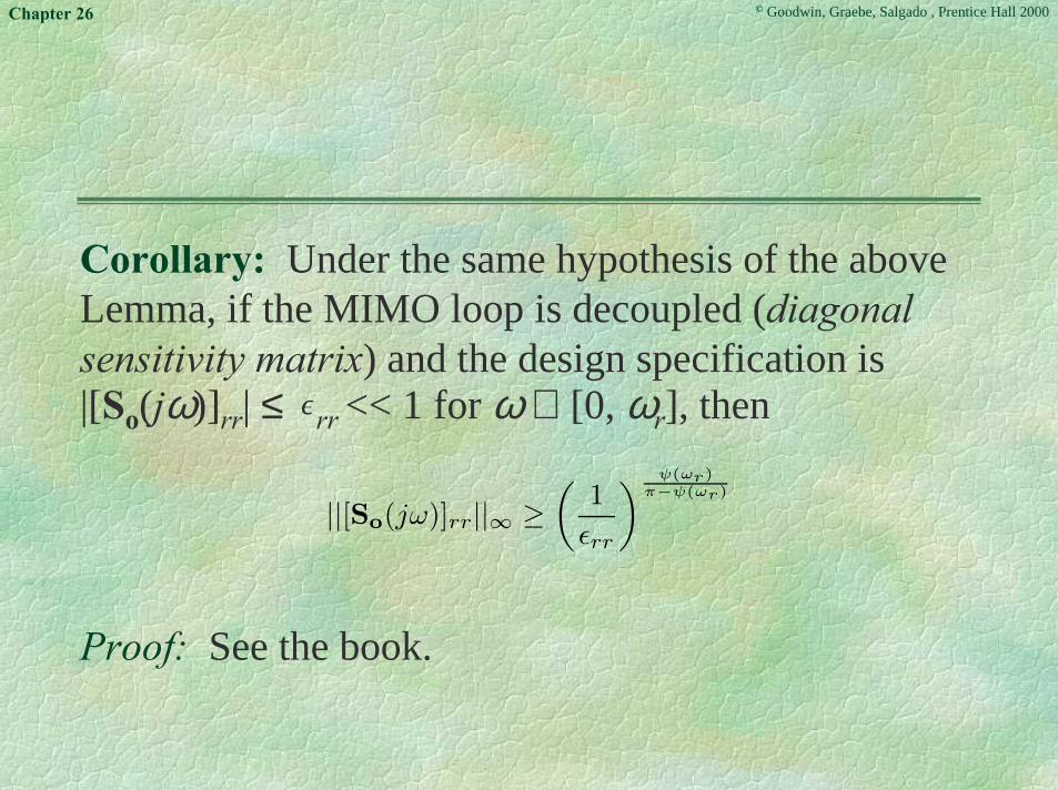
Corollary: Under the same hypothesis of the aboveLemma, if the MIMO loop is decoupled (diagonalsensitivity matrix) and the design specification is|[So(jω)]rr| ≤ rr << 1 for ω ∈ [0, ωr], then
Proof: See the book.
||[So(jω)]rr||∞ ≥(1εrr
) ψ(ωr)π−ψ(ωr)
© Goodwin, Graebe, Salgado , Prentice Hall 2000Chapter 26
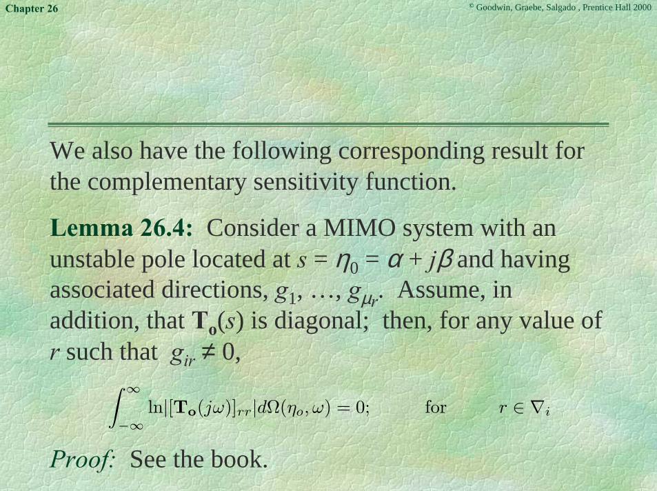
We also have the following corresponding result forthe complementary sensitivity function.
Lemma 26.4: Consider a MIMO system with anunstable pole located at s = η0 = α + jβ and havingassociated directions, g1, …, gµr. Assume, inaddition, that To(s) is diagonal; then, for any value ofr such that gir ≠ 0,
Proof: See the book.
∫ ∞
−∞ln|[To(jω)]rr|dΩ(ηo, ω) = 0; for r ∈ ∇i
© Goodwin, Graebe, Salgado , Prentice Hall 2000Chapter 26
The Cost of Decoupling
We can now investigate the cost of dynamicdecoupling, by comparing the results in Chapter 24with those in the above results. To make the analysismore insightful, we assume that the geometricmultiplicity µz of the zero is 1 - i.e., there is only oneleft direction, h1, associated with the particular zero.

© Goodwin, Graebe, Salgado , Prentice Hall 2000Chapter 26
We first assume that the left direction (h1) has morethan one element different from zero - i.e., that thecardinality ∇ i′ is larger than one. We then comparethe integral constraint applicable in the absence ofcoupling:
to the following integral constraint
(applicable to a dynamically decoupled MIMO loop).
∫ ∞
−∞ln |[So(jω)]rr| dΩ(zo, ω) ≥
∫ ∞
−∞ln
∣∣∣∣ hir[So(jω)]rr∑k∈∇′ hik[So(jω)]kr
∣∣∣∣ dΩ(zo, ω)
∫ ∞
−∞ln|[So(jω)]rr|dΩ(zo, ω) = 0; for r ∈ ∇′
i

© Goodwin, Graebe, Salgado , Prentice Hall 2000Chapter 26
In the first equation, we see that the right-hand side ofthe inequality can be negative for certain combinationsof nonzero off-diagonal sensitivities. Thus, it is feasibleto use off-diagonal sensitivities to reduce the lowerbound on the diagonal sensitivity peak. This can beinterpreted as a two-dimensional sensitivity trade-off,because it involves a spatial as well as a frequencydimension.

© Goodwin, Graebe, Salgado , Prentice Hall 2000Chapter 26
We recall that the capacity to use spatial interactionto reduce sensitivity peaks is a feature of MIMOsystems. The idea is that sensitivity dirt can beshared between outputs. This is shown in cartoonform on the next slide.

© Goodwin, Graebe, Salgado , Prentice Hall 2000Chapter 26
Spatial Allocation of Sensitivity
Sensitivity dirt Multiple piles

© Goodwin, Graebe, Salgado , Prentice Hall 2000Chapter 26
The conclusion from the above analysis is that it isless restrictive, from the point of view of designtrade-offs and constraints, to have an interactingMIMO control loop, compared to a dynamicallydecoupled one. However, it is a significant fact thatto draw these conclusions we relied on the fact that h1had more than one nonzero element. If that is not thecase, i.e., if only h1r ≠ 0 (the corresponding directionis canonical), then there is no additional trade-offimposed by requiring a decoupled closed loop.

© Goodwin, Graebe, Salgado , Prentice Hall 2000Chapter 26
Example
Consider the following MIMO system:
where
Go(s) =
1− s
(s+ 1)2s+ 3
(s+ 1)(s+ 2)
1− s
(s+ 1)(s+ 2)s+ 4(s+ 2)2
= GoN(s)[GoD(s)]−1I
GoN(s) =[
(1− s)(s+ 2)2 (s+ 1)(s+ 2)(s+ 3)(1− s)(s+ 2)(s+ 3) (s+ 1)2(s+ 4)
]
GoD(s) = (s+ 1)2(s+ 2)2

© Goodwin, Graebe, Salgado , Prentice Hall 2000Chapter 26
ZerosThe zeros of the plant are the roots of det(GoN(s)) - i.e.,the roots of -s6 - 11s5 - 43s4 - 63s3 + 74s + 44. Only oneof these roots, namely the one located at s = 1, lies inthe RHP. Thus, z0 = 1, and
We then compute Go(1) as
From which it can be seen that the dimension of the nullspace is µz = 1 and the (only) associated (left) directionis hT = [5 - 6].
dΩ(zo, ω) =1
1 + ω2dω
Go(1) =
[0 2
3
0 59
]

© Goodwin, Graebe, Salgado , Prentice Hall 2000Chapter 26
Clearly, this vector has two nonzero elements, so wecould expect that there will be additional designtrade-offs arising from decoupling. (The direction ofthe RHP zero is not canonical).
© Goodwin, Graebe, Salgado , Prentice Hall 2000Chapter 26
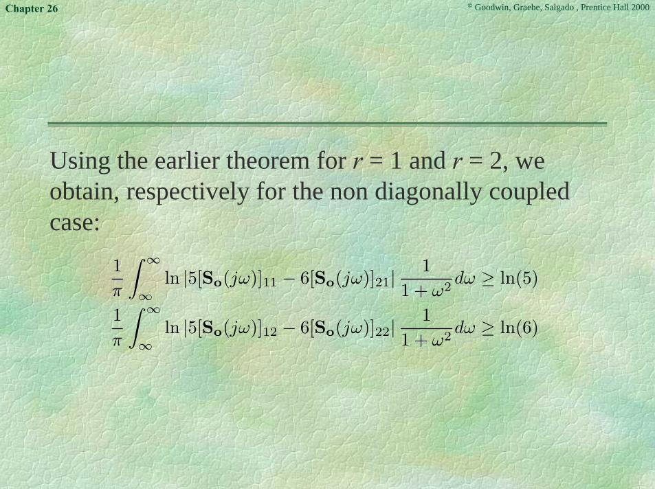
Using the earlier theorem for r = 1 and r = 2, weobtain, respectively for the non diagonally coupledcase:
1π
∫ ∞
∞ln |5[So(jω)]11 − 6[So(jω)]21|
11 + ω2
dω ≥ ln(5)
1π
∫ ∞
∞ln |5[So(jω)]12 − 6[So(jω)]22|
11 + ω2
dω ≥ ln(6)

© Goodwin, Graebe, Salgado , Prentice Hall 2000Chapter 26
If we impose typical design requirements, we have,for the interacting MIMO loop, that
1π
∫ ∞
∞ln |5[So(jω)]11 − 6[So(jω)]21|
11 + ω2
dω ≥ ln(5)
1π
∫ ∞
∞ln |5[So(jω)]12 − 6[So(jω)]22|
11 + ω2
dω ≥ ln(6)

© Goodwin, Graebe, Salgado , Prentice Hall 2000Chapter 26
If we require dynamic decoupling, the sensitivityintegrals become
With dynamic decoupling and typical designrequirements, we have
1π
∫ ∞
∞ln |[So(jω)]11|
11 + ω2
dω ≥ 0
1π
∫ ∞
∞ln |[So(jω)]22|
11 + ω2
dω ≥ 0
‖[So]11‖∞ ≥(1ε11
) ψ(ωc)π−ψ(ωc)
‖[So]22‖∞ ≥(1ε22
) ψ(ωc)π−ψ(ωc)

© Goodwin, Graebe, Salgado , Prentice Hall 2000Chapter 26
To quantify the relationship between the magnitude ofthe bounds in the coupled and the decoupled situations,we use an indicator κ1d, formed as the quotient betweenthe right-hand sides of inequalities
and
‖[So]11‖∞ +65‖[So]21‖∞ ≥
(1
ε11 + 65ε21
) ψ(ωc)π−ψ(ωc)
‖[So]22‖∞ +56‖[So]12‖∞ ≥
(1
ε22 + 56ε21
) ψ(ωc)π−ψ(ωc)
‖[So]11‖∞ ≥(1ε11
) ψ(ωc)π−ψ(ωc)
‖[So]22‖∞ ≥(1ε22
) ψ(ωc)π−ψ(ωc)

© Goodwin, Graebe, Salgado , Prentice Hall 2000Chapter 26
It follows that the indicator of the cost of decouplingis given by:
Thus, λ1 is a relative measure of interaction in thedirection from channel 1 to channel 2.
κ1d=
(1 +
65λ1ε
)− ψ(ωc)π−ψ(ωc)
where λ1ε=
ε21ε11

© Goodwin, Graebe, Salgado , Prentice Hall 2000Chapter 26
The issues discussed above are captured in graphicalform in the following figure.
Figure 26.10: Cost of decoupling in terms of sensitivity-peak lower bounds
0 1 2 3 4 5 6 7 8 9 100
0.2
0.4
0.6
0.8
1
1.2
Ratio λ1ε
=ε1/ε
2
Rat
io κ
1d
ωc=0.1
ωc=0.3
ωc=0.5
ωc=1.0

© Goodwin, Graebe, Salgado , Prentice Hall 2000Chapter 26
In the above figure, we show a family of curves, eachcorresponding to a different bandwidth ωc. Eachcurve represents, for the specified bandwidth, theratio between the bounds for the sensitivity peaks asa function of the decoupling indicator, λ1. We cansummarize our main observations as follows:
a) When λ1 is very small, there is virtually no effectof channel 1 into channel 2 (at least in the frequency band [0, ωc]); then, the bounds are very close (κ1d ≈ 1).

© Goodwin, Graebe, Salgado , Prentice Hall 2000Chapter 26
b) As λ1 increases, we are allowing the off-diagonal sensitivity to become larger than thediagonal sensitivity in [0, ωc]). The effect of thismanifests itself in κ1d < 1, i.e. in bounds for thesensitivity peak that are smaller than for thedecoupled situation.
c) If we keep λ1 fixed and we increase thebandwidth, then the advantages of using acoupled system also grow.

© Goodwin, Graebe, Salgado , Prentice Hall 2000Chapter 26
We see, from the above example, that decoupling canbe relatively cost-free, depending upon thebandwidth over which one requires that the closed-loop system operate. This is in accord with intuition,because zeros become significant only when onepushes the bandwidth beyond their locations.

© Goodwin, Graebe, Salgado , Prentice Hall 2000Chapter 26
We illustrate this conclusion for the system describedabove.Consider the plant
which has an ORHP zero at s = 1 with output directionequal to Ψ* = [5, -6].Since this direction is not canonical, we can argue fromthe preceding discussion that there will be a cost insensitivity associated with achieving diagonal decoupling.
=
++
++−
+++
+−
2)2(4
)2)(1(1
)2)(1(3
2)1(1
)(ss
sss
sss
ss
sG
© Goodwin, Graebe, Salgado , Prentice Hall 2000Chapter 26
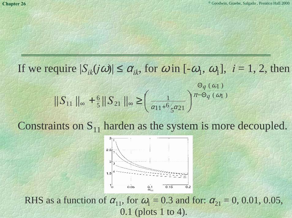
If we require |Sik(jω)| ≤ αik, for ω in [-ω1, ω1], i = 1, 2, then
Constraints on S11 harden as the system is more decoupled.
RHS as a function of α11, for ω1 = 0.3 and for: α21 = 0, 0.01, 0.05,0.1 (plots 1 to 4).
)1()1(
2156111
2156
11 |||||||| ωπω
ααq
q
SS Θ−Θ
+∞∞
≥+

© Goodwin, Graebe, Salgado , Prentice Hall 2000Chapter 26
We now apply a particular design technique, (we willnot go into details of the design, but λ = 1 gives fulldynamic decoupling and λ = 0 gives a triangulardesign) that allows different degrees of decouplingwhile keeping other design parameters essentiallyconstant. The resultant S is
=
+++
+
−−−
+
++++
3)1(4233
5)1(3
)22131643)(1(
3)1(
)31()2(230
)(s
ssss
sss
s
sss
sSλ
λλ

© Goodwin, Graebe, Salgado , Prentice Hall 2000Chapter 26
The next slide shows the effect of the extent ofdecoupling (measured by λ) on the magnitude of thesensitivity S11(jω).
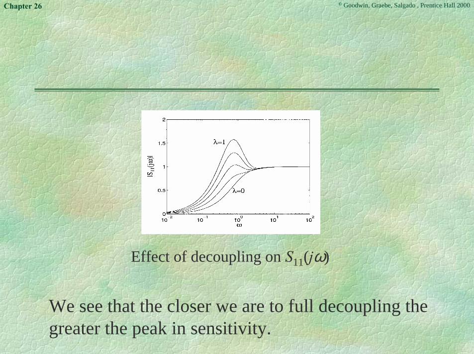
© Goodwin, Graebe, Salgado , Prentice Hall 2000Chapter 26
Effect of decoupling on S11(jω)
We see that the closer we are to full decoupling thegreater the peak in sensitivity.
© Goodwin, Graebe, Salgado , Prentice Hall 2000Chapter 26
Summary of Cost of Decoupling Depending on directionality properties of the zero-pole
structure of the plant, design constraints in MIMO mayrelax with respect to the SISO case (the cost of ORHP zerosand poles is distributed in S or T).
If the zero direction is not canonical, there is an additionalcost associated to decoupling, as restrictions concentrate onthe diagonal elements.
If the zero direction is canonical, the system is structurallyequivalent to the SISO system, in terms of constraints.There is no additional cost associated with decoupling.
© Goodwin, Graebe, Salgado , Prentice Hall 2000Chapter 26
Input Saturation
Finally, we explore the impact that input saturationhas on linear controllers that enforce decoupling. Wewill also develop anti-wind-up mechanisms thatpreserve decoupling in the face of saturation, usingmethods that are the MIMO equivalent of the SISOanti-wind-up methods of Chapter 11.
© Goodwin, Graebe, Salgado , Prentice Hall 2000Chapter 26
We assume that our plant is modeled as a squaresystem, with input u(t) ∈ m and output y(t) ∈ m.We also assume that the plant input is subject tosaturation. Then if u(i)(t) corresponds to the plantinput in the ith channel, i = 1, 2, …, m, the saturationis described by
u(i)(t) = Sat〈u(i)(t)〉 =
u(i)max if u(i)(t) > u
(i)max,
u(i)(t) if u(i)min ≤ u(i)(t) ≤ u
(i)max,
u(i)min if u(i)(t) < u
(i)min.

© Goodwin, Graebe, Salgado , Prentice Hall 2000Chapter 26
For simplicity of notation, we further assume that thelinear region is symmetrical with respect to theorigin, i.e. i = 1, 2, …, m. Wewill describe the saturation levels by usat ∈ m, where
The essential problem with input constraints, as inChapter 11, is that the control signal can wind upduring periods of saturation.
,|||| )()(max
)(min
isat
ii uuu ==
usat=
[u
(1)sat u
(2)sat . . . u
(m)sat
]T

© Goodwin, Graebe, Salgado , Prentice Hall 2000Chapter 26
MIMO Anti-Wind-Up Mechanism
In Chapter 11, the wind-up problems were dealt with byusing a particular implementation of the controller.This idea can be easily extended to the MIMO case, asfollows.
Assume that the controller transfer-function matrix,C(s), is biproper- i.e.,
where C∞ is nonsingular. The multivariable version ofthe anti-wind-up scheme if as shown on the next slide.
∞∞→
=CC )(lim ss

© Goodwin, Graebe, Salgado , Prentice Hall 2000Chapter 26
Figure 26.11: Anti-wind-up controller implementation.MIMO case
v(t)
elementNonlinearC1
[C(s)]−1 − [C1]−1
+ −
e(t) u(t) u(t)

© Goodwin, Graebe, Salgado , Prentice Hall 2000Chapter 26
In the scalar case, we found that the nonlinear elementcould be thought of in many different ways - e.g., as asimple saturation or as a reference governor. However,for SISO problems, all these procedures turn out to beequivalent. In the MIMO case, subtle issues arise fromthe way that the desired control, û(t), is projected intothe allowable region. We will explore threepossibilities.
(i) simple saturation(ii) input scaling(iii) error scaling

© Goodwin, Graebe, Salgado , Prentice Hall 2000Chapter 26
Simple saturation: Input saturation is the directanalog of the scalar case.
Input scaling: Here, compensation is achieved byscaling down the controller output vector û(t) to anew vector βû(t), every time that one (or more)component of û(t) exceeds its correspondingsaturation level. The scaling factor, β, is chosen insuch a way that u(t) = βû(t) - i.e., the controller isforced to come back just to the linear operation zone.This idea is shown schematically below.

© Goodwin, Graebe, Salgado , Prentice Hall 2000Chapter 26
Figure 26.12: Scheme to implement the scaling of controller outputs
Sat〈〉e(t) u(t)
−+
h〈〉
βI
usat
[C(s)]−1 − [C1 ]−1
C1
abs〈〉
u(t) βu(t)
−+
(In the above figure C1 should be C∞)

© Goodwin, Graebe, Salgado , Prentice Hall 2000Chapter 26
Error scaling: The third scheme is built by scalingthe error vector down to bring the loop just into thelinear region. We refer to the following slide.

© Goodwin, Graebe, Salgado , Prentice Hall 2000Chapter 26
Figure 26.13: Implementation of anti-wind-up via error scaling
Sat〈〉e(t)
u(t)
+
−αI
u(t)
[C(s)]−1 − [C1 ]−1
C1
abs〈〉
−+
usat
w2(t) = αe(t)
w1(t)
f〈〉
(In the above figure C1 should be C∞)

© Goodwin, Graebe, Salgado , Prentice Hall 2000Chapter 26
Note that û can be changed only instantaneously bymodifying w2, because w1(t) is generated through astrictly proper transfer function. Hence, the scaling ofthe error is equivalent to bringing w2 to a value suchthat û is just inside the linear region.

© Goodwin, Graebe, Salgado , Prentice Hall 2000Chapter 26
In Figure 26.13, the block f denotes a function thatgenerates the scaling factor 0 < α < 1. We observe thatthe block with transfer-function matrix [C(s)-1] - C∞ isstrictly proper, so that any change in the error vectore(t) will translate immediately into a change in thevector û(t). Instead of introducing abrupt changes ine(t) (and thus in û(t), a gentler strategy can be used. Anexample of this strategy is to generate α as the outputof a first-order dynamic system with unit d.c. gain, timeconstant τ, and initial condition α(0) = 1.

© Goodwin, Graebe, Salgado , Prentice Hall 2000Chapter 26
Figure 26.14: Effects of different techniques for dealing with saturation in MIMO systems
u(1)sat
u(2)
uus
uu
w1
ue
u(1)
w2
û : raw control signalus : control signal which results from directly saturating u(1)
uu : control signal obtained with the scaled control technique(as in Figure 26.12)
ue : control signal obtained with the scaled error technique (asin Figure 26.13)

© Goodwin, Graebe, Salgado , Prentice Hall 2000Chapter 26
Example
Consider a MIMO process having the nominal model
with
+−−++−
++= 23
122)42(
1)( 2 sss
sssoG
22
2
)42(72))(det(
++++=
sssssoG

© Goodwin, Graebe, Salgado , Prentice Hall 2000Chapter 26
Note that this model is stable and minimum phase.Therefore, dynamic decoupling is possible withoutsignificant difficulties.
A suitable decoupling controller is
C(s) =2(s+ 2)(s2 + 2s+ 4)s(s+ 1)(s2 + 2s+ 7)
[−s+ 2 −2s− 13 −s+ 2
]

© Goodwin, Graebe, Salgado , Prentice Hall 2000Chapter 26
We first run a simulation that assumes that there is noinput saturation. The results are shown below. Observethat full dynamic decoupling has indeed been achieved.
Figure 26.15: Decoupled design in the absence of saturation
0 2 4 6 8 10 12 14 16 18 200
0.5
1
1.5
2
Time [s]
Pla
nt o
utpu
ts a
nd r
ef.
y1(t)
y2(t)
© Goodwin, Graebe, Salgado , Prentice Hall 2000Chapter 26
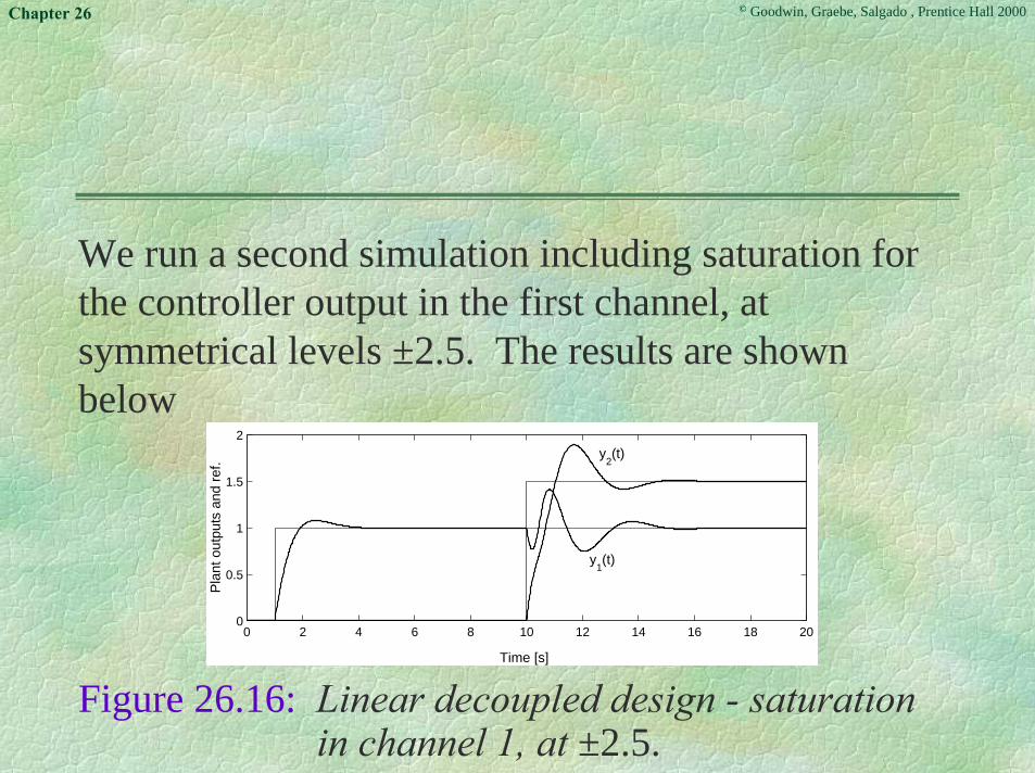
We run a second simulation including saturation forthe controller output in the first channel, atsymmetrical levels ±2.5. The results are shownbelow
Figure 26.16: Linear decoupled design - saturation in channel 1, at ±2.5.
0 2 4 6 8 10 12 14 16 18 200
0.5
1
1.5
2
Time [s]
Pla
nt o
utpu
ts a
nd r
ef.
y1(t)
y2(t)

© Goodwin, Graebe, Salgado , Prentice Hall 2000Chapter 26
Clearly, the results are very poor. This is due towind-up effects and stray coupling in the controllerthat occur during saturation but which have not beencompensated. We therefore explore anti-wind-upprocedures.
We example the three anti-wind-up proceduresdescribed above.

© Goodwin, Graebe, Salgado , Prentice Hall 2000Chapter 26
Simple saturation: The results of simply putting asaturation element into the nonlinear element of theMIMO anti-windup current are shown on the nextslide. It can be seen that this is unsatisfactory -indeed, the results are similar to those where no anti-wind-up mechanism was used.

© Goodwin, Graebe, Salgado , Prentice Hall 2000Chapter 26
Figure 26.17: Decoupled linear design with saturation in channel 1 and anti-wind-up scheme
0 2 4 6 8 10 12 14 16 18 20−0.5
0
0.5
1
1.5
2
Time [s]
Pla
nt o
utpu
ts a
nd r
ef.
y2(t)
y1(t)

© Goodwin, Graebe, Salgado , Prentice Hall 2000Chapter 26
Input scaling: A rather disappointing result isobserved regarding the plant outputs. They areshown on the next slide.
The results show only a marginal improvement overthose obtained by using the pure anti-wind-upmechanism.

© Goodwin, Graebe, Salgado , Prentice Hall 2000Chapter 26
Figure 26.19: Plant outputs when using control scaling
0 2 4 6 8 10 12 14 16 18 20−0.5
0
0.5
1
1.5
2
Time [s]
Pla
nt o
utpu
ts a
nd r
ef.
y2(t)
y1(t)

© Goodwin, Graebe, Salgado , Prentice Hall 2000Chapter 26
Error scaling: When the error-scaling strategy isapplied to our example, we obtain the results shownon the next slide.

© Goodwin, Graebe, Salgado , Prentice Hall 2000Chapter 26
Figure 26.20: Plant outputs when using scaled errors
0 2 4 6 8 10 12 14 16 18 200
0.5
1
1.5
2
Time [s]
Pla
nt o
utpu
ts a
nd r
ef.
y1(t)
y2(t)

© Goodwin, Graebe, Salgado , Prentice Hall 2000Chapter 26
The results are remarkably better than those producedby the rest of the strategies treated so far. Actually,full dynamic decoupling is essentially retained here -the small coupling evident, is due to theimplementation of the error scaling via a (fast)dynamical system.

© Goodwin, Graebe, Salgado , Prentice Hall 2000Chapter 26
Summary Recall these key closed-loop specifications shared by SISO
and MIMO design: continued compensation of disturbances continued compensation of model uncertainty stabilization of open-loop unstable systems
whilst not becoming too sensitive to measurement noise generating excessive control signals
and accepting inherent limitations due to unstable zeros unstable poles modeling error frequency- and time-domain integral constraints

© Goodwin, Graebe, Salgado , Prentice Hall 2000Chapter 26
Generally, MIMO systems also exhibit additionalcomplexities due to
directionality (several inputs acting on one output) dispersion (one input acting on several outputs) and the resulting phenomenon of coupling.
Designing a controller for closed-loop compensation of thisMIMO coupling phenomenon is called decoupling.
Recall that there are different degrees of decoupling,including the following:
static (i.e., To(0) is diagonal); triangular (i.e., To(s) is triangular); and dynamic (i.e., To(s) is diagonal).

© Goodwin, Graebe, Salgado , Prentice Hall 2000Chapter 26
Due to the fundamental law that So(s) + To(s) = I, if Toexhibits any of these decoupling properties, so does So.
The severity and types of the trade-offs associated withdecoupling depend on
whether the system is minimum phase; the directionality and cardinality of nonminimum-phase zeros; unstable poles.
If all of the system’s unstable zeros are canonical (theirdirectionality affects one output only), then their adverseeffect is not spread to other channels by decoupling,provided that the direction of decoupling is congruent withthe direction of the unstable zeros.

© Goodwin, Graebe, Salgado , Prentice Hall 2000Chapter 26
The price for dynamically decoupling a system havingnoncanonical nonminimum-phase zeros of simplemultiplicity is that
the effect of the nonminimum-phase zeros is potentially spreadacross several loops; and,
therefore, although the loops are decoupled, each of the affectedloops needs to observe the bandwidth and sensitivity limitationsimposed by the unstable zero dynamics.
If one accepts the less stringent triangular decoupling, theeffect of dispersing limitations due to nonminimum-phasezeros can be minimized.

© Goodwin, Graebe, Salgado , Prentice Hall 2000Chapter 26
Depending on the case, a higher cardinality ofnonminimum-phase zeros can either enforce or mitigate theadverse effects.
If a system is also open-loop unstable, there may not be anyway at all to achieve full dynamic decoupling with a one-d.o.f. controller, although it is always possible with a two-d.o.f. architecture for reference-signal changes.
If a system is essentially linear but exhibits such actuatornonlinearities as input or slew-rate saturations, then thecontroller design must reflect this appropriately.

© Goodwin, Graebe, Salgado , Prentice Hall 2000Chapter 26
Otherwise, the MIMO generalization of the SISO wind-upphenomenon can occur.
MIMO wind-up manifests itself in two aspects ofperformance degradation:
transients due to growing controller states; and transients due to the nonlinearity impacting on directionality.

© Goodwin, Graebe, Salgado , Prentice Hall 2000Chapter 26
The first of these two phenomena …… is analogous to the SISO case.
… is due to the saturated control signals not being able to annihilate thecontrol errors sufficiently fast compared to the controller dynamics;therefore the control states continue to grow in response to thenondecreasing control. These wound up states produce the transientswhen the loop emerges from saturation.
… can be compensated by a direct generalization of the SISO anti-wind-up implementation.
The second phenomena …… is specific to MIMO systems.
… is due to uncompensated interactions arising from the input vectorslosing its original design direction.

© Goodwin, Graebe, Salgado , Prentice Hall 2000Chapter 26
Analogously to the SISO case, there can be regions in statespace from which an open-loop unstable MIMO systemwith input saturation cannot be stabilized by any control.
More severely than in the SISO case, MIMO systems aredifficult to control in the presence of input saturation, evenif the linear loop is stable and the controller is implementedwith anti-wind-up. This is due to saturation changing thedirectionality of the input vector.
This problem of preserving decoupling in the presence ofinput saturation can be addressed by anti-wind-up schemesthat scale the control error rather than the control signal.