Chapter 26 Part 1COMPARING COUNTS

Is an observed distribution consistent with what we expect?

Are observed differences among several distributions large enough to be significant?

These are questions that we will answer using a (chi-squared) model.

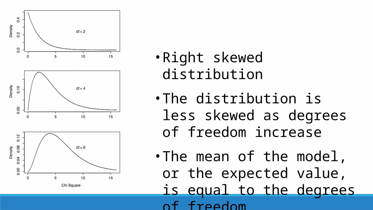
• Right skewed distribution

• The distribution is less skewed as degrees of freedom increase

• The mean of the model, or the expected value, is equal to the degrees of freedom

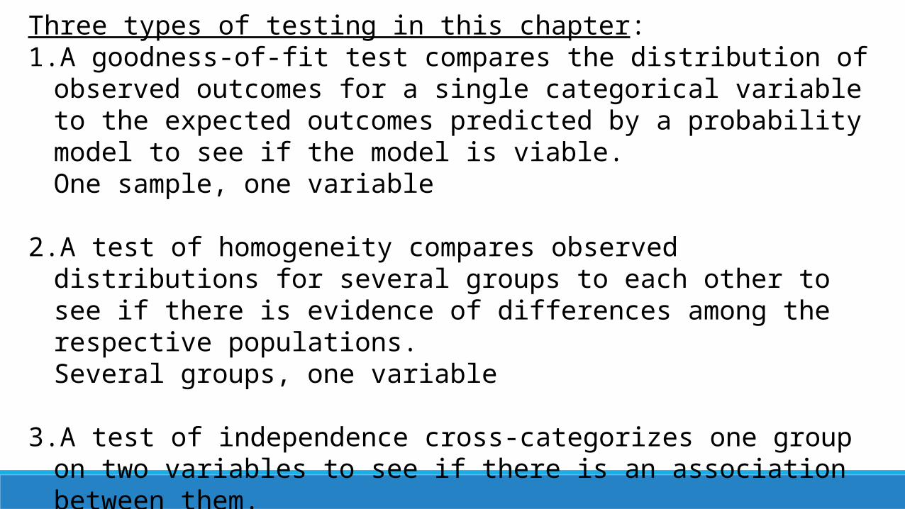
Three types of testing in this chapter: 1. A goodness-of-fit test compares the distribution of observed outcomes for a

single categorical variable to the expected outcomes predicted by a probability model to see if the model is viable. One sample, one variable

2. A test of homogeneity compares observed distributions for several groups to each other to see if there is evidence of differences among the respective populations. Several groups, one variable

3. A test of independence cross-categorizes one group on two variables to see if there is an association between them. One sample, two variables

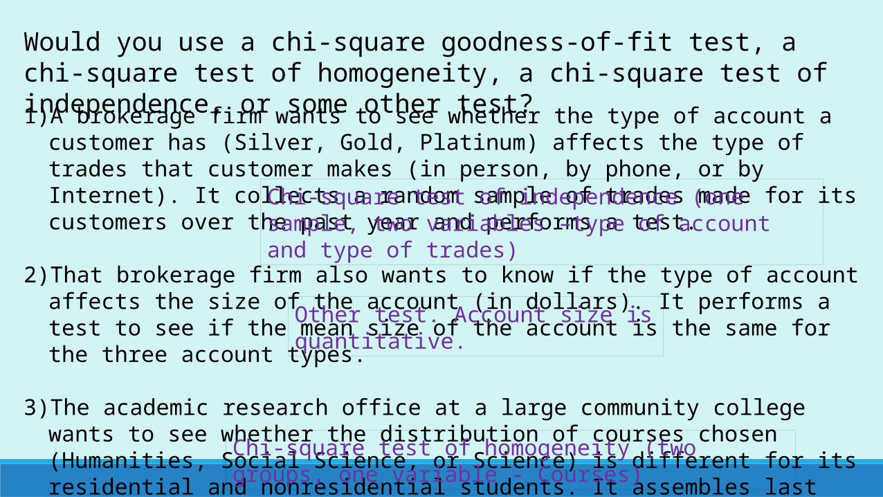
Would you use a chi-square goodness-of-fit test, a chi-square test of homogeneity, a chi-square test of independence, or some other test?

1) A brokerage firm wants to see whether the type of account a customer has (Silver, Gold, Platinum) affects the type of trades that customer makes (in person, by phone, or by Internet). It collects a random sample of trades made for its customers over the past year and performs a test.

2) That brokerage firm also wants to know if the type of account affects the size of the account (in dollars). It performs a test to see if the mean size of the account is the same for the three account types.

3) The academic research office at a large community college wants to see whether the distribution of courses chosen (Humanities, Social Science, or Science) is different for its residential and nonresidential students. It assembles last semester’s data and performs a test.

Chi-square test of independence (one sample, two variables –type of account and type of trades)

Other test. Account size is quantitative.

Chi-square test of homogeneity (two groups, one variable - Courses)

tests are only appropriate for

categorical data!

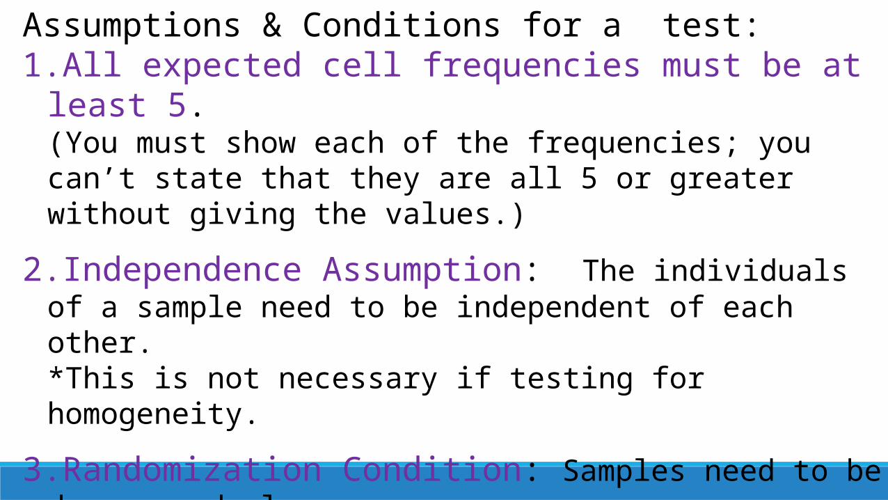
Assumptions & Conditions for a test: 1.All expected cell frequencies must be at least 5.

(You must show each of the frequencies; you can’t state that they are all 5 or greater without giving the values.)

2.Independence Assumption: The individuals of a sample need to be independent of each other. *This is not necessary if testing for homogeneity.

3.Randomization Condition: Samples need to be drawn randomly.

4.Counted Data Condition: The data must be counts or frequencies.

Placebo St John’s Wort PosrexDepression returned

24 22 14

No sign of depression

6 8 16

Medical researchers enlisted 90 subjects for an experiment comparing treatments for depression. The subjects were randomly divided into three groups and given pills to take for a period of three months. Unknown to them, one group received a placebo, the second group the “natural” remedy St. John’s Word, and the third group the prescription drug Posrex. After six months, psychologists and physicians evaluated the subjects to see if their depression has returned.

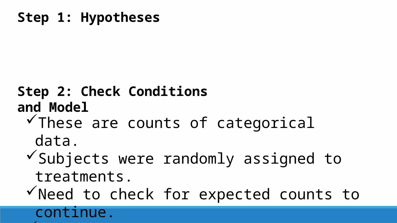
Step 1: Hypotheses

Step 2: Check Conditions and Model

These are counts of categorical data. Subjects were randomly assigned to treatments. Need to check for expected counts to continue. The degrees of freedom = (#rows – 1)(#columns -1)

Checking expected counts…

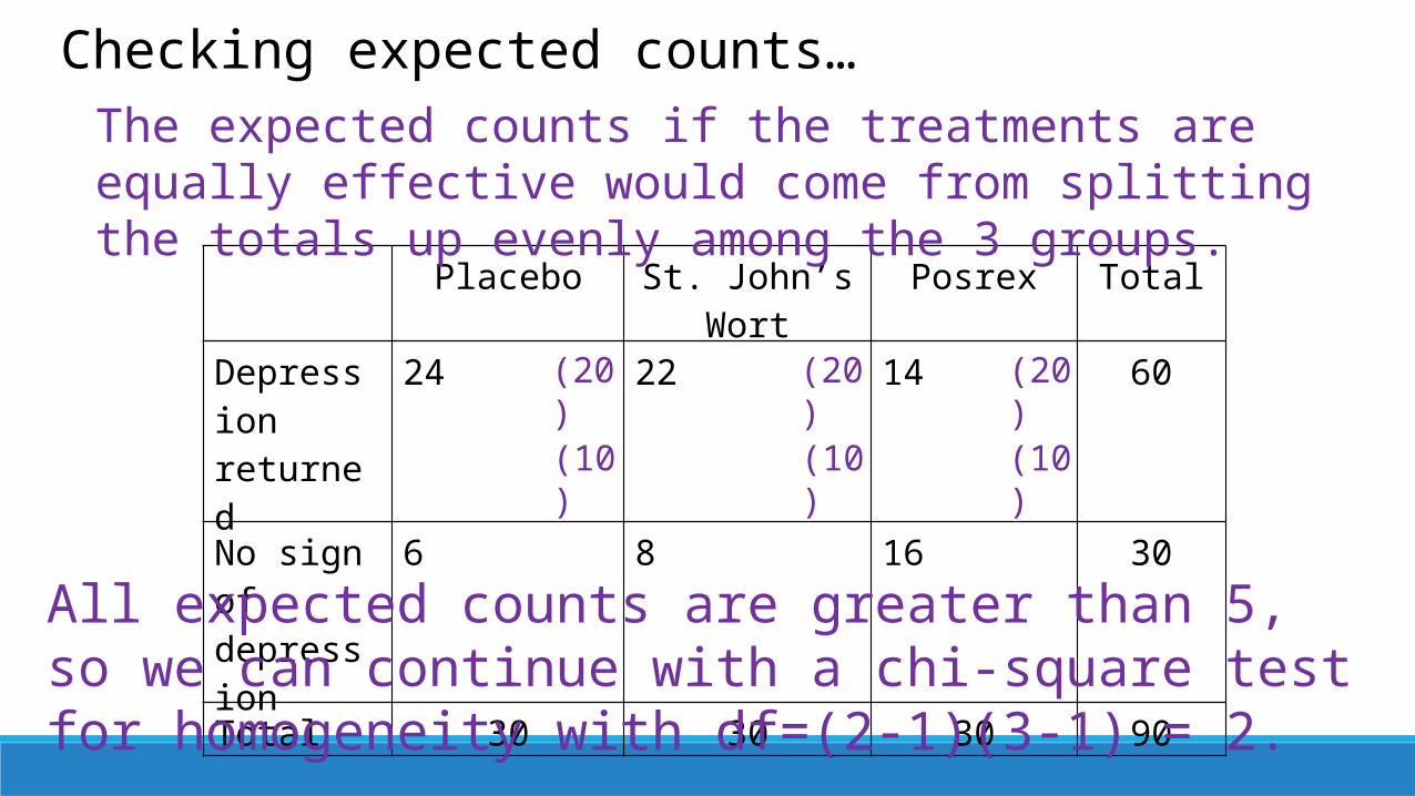
Placebo St. John’s Wort Posrex TotalDepression returned

24 22 14 60

No sign of depression

6 8 16 30

Total 30 30 30 90

The expected counts if the treatments are equally effective would come from splitting the totals up evenly among the 3 groups.

(20) (20) (20)

(10) (10) (10)

All expected counts are greater than 5, so we can continue with a chi-square test for homogeneity with df=(2-1)(3-1) = 2.

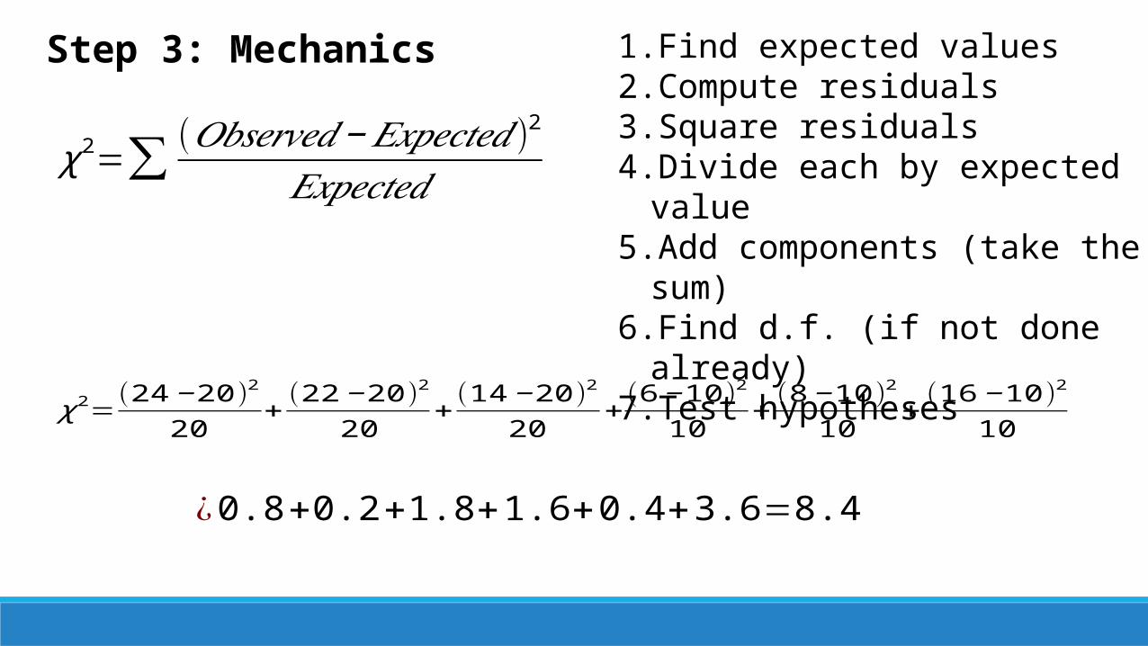
Step 3: Mechanics

χ 2=∑ (𝑂𝑏𝑠𝑒𝑟𝑣𝑒𝑑−𝐸𝑥𝑝𝑒𝑐𝑡𝑒𝑑)2

𝐸𝑥𝑝𝑒𝑐𝑡𝑒𝑑

1. Find expected values 2. Compute residuals 3. Square residuals 4. Divide each by expected value 5. Add components (take the sum) 6. Find d.f. (if not done already) 7. Test hypotheses

χ 2=(24−20)2

20+(22−20)2

20+(14−20)2

20+

(6−10)2

10+(8−10)2

10+(16−10)2

10

¿0.8+0.2+1.8+1.6+0.4+3.6=8.4

To get the P-value on TI-84:

DIST 8:cdf ( score, 999, df)

*We always do a right-tail test for chi-square

𝑃 ( χ 2>8.4 )=0.015

Step 4: Conclusion

Because the P-value is low, we reject the null hypothesis. There is strong evidence that the tested treatments are not all equally effective in preventing the recurrence of depression. It appears that people who took the prescription drug Posrex are more likely to remain free of the signs of depression than those who took a placebo or the natural remedy St. John’s wort.

Assignment: Due Today - Ch 26 HW Pt 1 - Page 642 #2-4Chapter 26 Quiz April 30 (In Class)