Chapter 26: Spatio-temporal models for EEG

W. Penny, N. Trujillo-Barreto and E. Aubert

May 25, 2006

Introduction

Imaging neuroscientists have at their disposal a variety of imaging techniques forinvestigating human brain function [Frackowiak et al. 2003]. Among these, theElectroencephalogram (EEG) records electrical voltages from electrodes placedon the scalp, the Magnetoencephalogram (MEG) records the magnetic field fromsensors placed just above the head and functional Magnetic Resonance Imaging(fMRI) records magnetisation changes due to variations in blood oxygenation.

However, as the goal of brain imaging is to obtain information about theneuronal networks that support human brain function, one must first transformmeasurements from imaging devices into estimates of intracerebral electrical ac-tivity. Brain imaging methodologists are therefore faced with an inverse prob-lem, ‘How can one make inferences about intracerebral neuronal processes givenextracerebral or vascular measurements ?’

We argue that this problem is best formulated as a model-based spatio-temporal deconvolution problem. For EEG and MEG the required deconvolu-tion is primarily spatial, and for fMRI it is primarily temporal. Although onecan make minimal assumptions about the source signals by applying ‘blind’ de-convolution methods [Makeig et al. 2002, McKeown et al. 1998], knowledge ofthe underlying physical processes can be used to great effect. This informationcan be implemented in a forward model that is inverted during deconvolution.In M/EEG, forward models make use of Maxwell’s equations governing prop-agation of electromagnetic fields [Baillet et al. 2001], and, in fMRI hemody-namic models that link neural activity to ‘Balloon’ models of vascular dynamics[Friston et al. 2000].

To implement a fully spatio-temporal deconvolution, time-domain fMRImodels must be augmented with a spatial component and spatial-domain M/EEGmodels with a temporal component. The previous Chapter showed how thiscould be implemented for fMRI. This Chapter describes a model-based spatio-temporal deconvolution method for M/EEG.

The underlying forward or ‘generative’ model incorporates two mappings.The first specifies a time-domain General Linear Model (GLM) at each pointin source space. This relates effects of interest at each voxel to source activityat that voxel. This is identical to the ‘mass-univariate’ approach that is widelyused in the analysis of fMRI [Frackowiak et al. 2003]. The second mappingrelates source activity to sensor activity at each time point using the usualspatial-domain lead-field matrix (see Chapter 28).

Our model therefore differs from the standard generative model implicit insource reconstruction by having an additional level that embodies temporal

1

priors. There are two potential benefits of this approach. First, the use of tem-poral priors can result in more sensitive source reconstructions. This may allowsignals to be detected that cannot be detected otherwise. Second, it providesan analysis framework for M/EEG that is very similar to that used in fMRI.The experimental design can be coded in a design matrix, the model fittedto data, and various effects of interest can be characterised using ‘contrasts’[Frackowiak et al. 2003]. These effects can then be tested for statistically usingPosterior Probability Maps (PPMs), as described in previous Chapters. Impor-tantly, the model does not need to be refitted to test for multiple experimentaleffects that are potentially present in any single data set. Sources are estimatedonce only using a spatio-temporal deconvolution rather than separately for eachtemporal component of interest.

The Chapter is organised as follows. In the Theory section we describethe model and relate it to existing distributed solutions. The success of theapproach rests on our ability to characterise neuronal responses, and task-relateddifferences in them, using GLMs. We describe how this can be implemented forthe analysis of ERPs and show how the model can be inverted to produce sourceestimates using Variational Bayes (VB). The framework is applied to simulateddata and data from an EEG study of face processing.

Theory

Notation

Lower case variable names denote vectors and scalars. Whether the variable isa vector or scalar should be clear from the context. Upper case names denotematrices or dimensions of matrices. In what follows N(x;µ, Σ) denotes a multi-variate normal density over x, having mean µ and covariance Σ. The precision ofa Gaussian variate is the inverse (co)variance. A gamma density over the scalarrandom variable x is written as Ga(x; a, b). Normal and Gamma densities aredefined in Chapter 26. We also use ||x||2 = xT x, denote the trace operator asTr(X), X+ for the pseudo-inverse, and use diag(x) to denote a diagonal matrixwith diagonal entries given by the vector x.

Generative Model

The aim of source reconstruction is to estimate Primary Current Density (PCD)J from measured M/EEG measurements Y . If we have m = 1..M sensors,g = 1..G sources and t = 1..T time points then J is of dimension G × T andY is of dimension M × T . The applications in this Chapter use a corticalsource space in which dipole orientations are constrained to be perpendicularto the cortical surface. Each entry in J therefore corresponds to the scalarcurrent density at particular locations and time points. Sensor measurementsare related to current sources via Maxwell’s equations governing electromagneticfields [Baillet et al. 2001] (see Chapter 28).

Most established distributed source reconstruction or ‘imaging’ methods

2

[Darvas et al. 2004] implicitly rely on the following two-level generative model

p(Y |J,Ω) =T∏

t=1

N(yt;Kjt,Ω) (1)

p(J |α) =T∏

t=1

N(jt; 0, α−1D−1)

where jt and yt are the source and sensor vectors at time t, K is the [M × G]lead-field matrix and Ω is the sensor noise covariance. The matrix D reflectsthe choice of spatial prior and α is a spatial precision variable. This generativemodel is shown schematically in Figure 1 and can be written as a hierarchicalmodel

Y = KJ + E (2)J = Z

(3)

in which random fluctuations E correspond to sensor noise and the source activ-ity is generated by random innovations Z. Critically, these assumptions provideempirical priors on the spatial deployment of source activity (see Chapter 29).

Because the number of putative sources is much greater than the number ofsensors, G >> M , the source reconstruction problem is ill-posed. Distributedsolutions therefore depend on the specification of a spatial prior for estimation toproceed. A common choice is the Laplacian prior used, for example, in Low Res-olution Electromagnetic Tomography (LORETA) [Pascual-Marqui et al. 1994].This can be implemented in the above generative model by setting D to com-pute local differences as measured by an L2-norm, which embodies a belief thatsources are diffuse and highly distributed. Other spatial priors, such as thosebased on L1-norms [Fuchs et al. 1999], Lp-norms [Auranen et al. 2005], or Vari-able Resolution Electromagnetic Tomography (VARETA) [Valdes-Sosa et al. 2000]can provide more focal source estimates. These are all examples of schemesthat use a single spatial prior and are special cases of a more general model[Mattout et al. 2006] that covers multiple priors. In this model the sensor noiseand spatial prior covariances are modelled as mixtures of components Ωi andQi respectively

p(Y |J,Ω) =T∏

t=1

N(yt;Kjt, ρ1Ω1 + ρ2Ω2 + ...) (4)

p(J |α) =T∏

t=1

N(jt; 0, γ1Q1 + γ2Q2 + ...)

The advantage of this model is that multiple priors can be specified and aremixed adaptively by adjusting the covariance parameters ρi and γi, as describedin Chapter 29. One can also use Bayesian model selection to compare differentcombinations of priors, as described in Chapter 35. For simplicity, we will dealwith a single spatial prior component because we want to focus on temporalpriors. However, it would be relatively simple to extend the approach to covermultiple prior covariance (or precision) components.

3

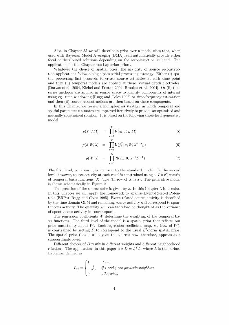
Also, in Chapter 35 we will describe a prior over a model class that, whenused with Bayesian Model Averaging (BMA), can automatically provide eitherfocal or distributed solutions depending on the reconstruction at hand. Theapplications in this Chapter use Laplacian priors.

Whatever the choice of spatial prior, the majority of source reconstruc-tion applications follow a single-pass serial processing strategy. Either (i) spa-tial processing first proceeds to create source estimates at each time pointand then (ii) temporal models are applied at these ‘virtual depth electrodes’[Darvas et al. 2004, Kiebel and Friston 2004, Brookes et al. 2004]. Or (ii) timeseries methods are applied in sensor space to identify components of interestusing eg. time windowing [Rugg and Coles 1995] or time-frequency estimationand then (ii) source reconstructions are then based on these components.

In this Chapter we review a multiple-pass strategy in which temporal andspatial parameter estimates are improved iteratively to provide an optimised andmutually constrained solution. It is based on the following three-level generativemodel

p(Y |J,Ω) =T∏

t=1

N(yt;Kjt,Ω) (5)

p(J |W,λ) =T∏

t=1

N(jTt ;xtW,λ−1IG) (6)

p(W |α) =K∏

k=1

N(wk; 0, α−1D−1) (7)

The first level, equation 5, is identical to the standard model. In the secondlevel, however, source activity at each voxel is constrained using a [T×K] matrixof temporal basis functions, X. The tth row of X is xt. The generative modelis shown schematically in Figure 2.

The precision of the source noise is given by λ. In this Chapter λ is a scalar.In this Chapter we will apply the framework to analyse Event-Related Poten-tials (ERPs) [Rugg and Coles 1995]. Event-related source activity is describedby the time domain GLM and remaining source activity will correspond to spon-taneous activity. The quantity λ−1 can therefore be thought of as the varianceof spontaneous activity in source space.

The regression coefficients W determine the weighting of the temporal ba-sis functions. The third level of the model is a spatial prior that reflects ourprior uncertainty about W . Each regression coefficient map, wk (row of W ),is constrained by setting D to correspond to the usual L2-norm spatial prior.The spatial prior that is usually on the sources now, therefore, appears at asuperordinate level.

Different choices of D result in different weights and different neighborhoodrelations. The applications in this paper use D = LT L, where L is the surfaceLaplacian defined as

Lij =

1, if i=j− 1

Nij, if i and j are geodesic neighbors

0, otherwise.

4

where Nij is the geometric mean of the number of neighbors of i and j. Thisprior has been used before in the context of fMRI with Euclidean neighbors[Penny and Flandin 2005, Woolrich et al. 2001].

The first level of the model assumes that there is Gaussian sensor noise, et,with zero mean and covariance Ω. This covariance can be estimated from pre-stimulus or baseline periods when such data are available [Sahani and Nagarajan 2004].Alternatively, we assume that Ω = diag(σ−1) where the mth element of σ−1 isthe noise variance on the mth sensor. We provide a scheme for estimating σm,should this be necessary.

We also place Gamma priors on the precision variables σ, λ and α

p(σ) =M∏

m=1

Ga(σm; bσprior, cσprior

) (8)

p(λ) = Ga(λ; bλprior, cλprior

)

p(α) =K∏

k=1

Ga(αk; bαprior, cαprior

)

This allows the inclusion of further prior information into the source localisa-tion. For example, instead of using baseline periods to estimate a full covariancematrix Ω we could use this data to estimate the noise variance at each sensor.This information could then be used to set bσprior and cσprior , allowing noise es-timates during periods of interest to be constrained softly by those from baselineperiods. Similarly, we may wish to enforce stronger or weaker spatial regular-isation on wk by setting bαprior

and cαpriorappropriately. The applications in

this Chapter, however, use uninformative gamma priors. This means that σ, λand α will be estimated solely from the data Y .

In summary, the addition of the supraordinate level to our generative modelinduces a partioning of source activity into signal and noise. We can see thisclearly by reformulating the probabilistic model as before

Y = KJ + E (9)JT = XW + Z

W = P

Here we have random innovations Z which are ‘temporal errors’, ie. lack offit of the temporal model, and P which are ‘spatial errors’, ie. lack of fit of aspatial model. Here the spatial model is simply a zero mean Gaussian with co-variance α−1D−1. We can regard XW as an empirical prior on the expectationof source activity. This empirical Bayes perspective means that the conditionalestimates of source activity J are subject to bottom-up constraints, providedby the data, and top-down predictions from the third-level of our model. Wewill use this heuristic later to understand the update equations used to estimatesource activity.

Temporal priors

The usefulness of the spatio-temporal approach rests on our ability to charac-terise neuronal responses using GLMs. Fortunately, there is a large literature

5

Figure 1: Generative model for source reconstruction. This is a graphical rep-resentation of the probabilistic model implicit in many distributed source solu-tions.

6

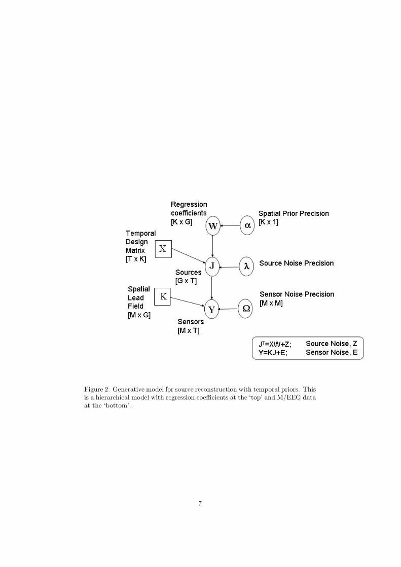
Figure 2: Generative model for source reconstruction with temporal priors. Thisis a hierarchical model with regression coefficients at the ‘top’ and M/EEG dataat the ‘bottom’.

7

that suggests this is possible. The type of temporal model necessary will dependon the M/EEG response one is interested in. These components could be (i) sin-gle trials, (ii) evoked components (steady-state or ERPs [Rugg and Coles 1995])or (iii) induced components [Tallon-Baudry et al. 1996].

In this Chapter we focus on ERPs. We briefly review three different ap-proaches for selecting an appropriate ERP basis set. These basis functions willform columns in the GLM design matrix, X (see equation 6 and figure 2).

Damped sinusoids

An ERP basis set can be derived from the fitting of Damped Sinusoidal (DS)components [Demiralp et al. 1998]. These are given by

j =K∑

k=1

wkxk (10)

xk = exp(iφk) exp(αk + i2πfk)δt

where i =√−1, δt is the sampling interval and wk, φk, αk and fk are the

amplitude, phase, damping and frequency of the kth component. The [T × 1]vector xk will form the kth column in the design matrix. Figure 3 shows howdamped sinusoids can generate an ERP.

Fitting DS models to ERPs from different conditions allows one to makeinferences about task related changes in constituent rhythmic components. Forexample, in [Demiralp et al. 1998], responses to rare auditory events elicitedhigher amplitude, slower delta and slower damped theta components than didresponses to frequent events. Fitting damped sinusoids, however, requires anonlinear estimation procedure. But approximate solutions can also be foundusing the Prony and related methods [Osborne and Smyth 1991] which requiretwo-stages of linear estimation.

Once a DS model has been fitted, for example to the principal componentof the sensor data, the components xk provide a minimal basis set. Includingextra regressors from a first-order Taylor expansion about phase, damping andfrequency ( ∂xk

∂φk, ∂xk

∂αk, ∂xk

∂fk) provides additional flexibility. Use of this expanded

basis in our model would allow these attributes to vary with source location.Such Taylor series expansions have been particularly useful in GLM character-isations of hemodynamic responses in fMRI [Frackowiak et al. 2003].

Wavelets

ERPs can also be modelled using wavelets

j =K∑

k=1

wkxk (11)

where xk are wavelet basis functions and wk are wavelet coefficients. Waveletsprovide a tiling of time-frequency space that gives a balance between timeand frequency resolution. The Q-factor of a filter or basis function is de-fined as the central frequency to bandwidth ratio. Wavelet bases are cho-sen to provide constant Q [Unser and Aldroubi 1996]. This makes them goodmodels of nonstationary signals, such as ERPs and induced EEG components

8

[Tallon-Baudry et al. 1996]. Wavelet basis sets are derived by translating anddilating a mother wavelet. Figure 4 shows wavelets from two different basissets, one based on Daubechies wavelets and one based on Battle-Lemarie (BL)wavelets. These basis sets are orthogonal. Indeed the BL wavelets have been de-signed from an orthogonalisation of cubic B-splines [Unser and Aldroubi 1996].

If K = T , then the mapping j → w is referred to as a wavelet transform,and for K > T we have an overcomplete basis set. More typically, we haveK ≤ T . In the ERP literature the particular subset of basis functions used ischosen according to the type of ERP component one wishes to model. Popularchoices are wavelets based on B-splines [Unser and Aldroubi 1996].

In statistics, however, it is well known that an appropriate subset of basisfunctions can be automatically selected using a procedure known as ‘waveletshrinkage’ or ‘wavelet denoising’. This relies on the property that natural sig-nals such as images, speech or neuronal activity can be represented using asparse code comprising just a few large wavelets coefficients. Gaussian noisesignals, however, produce Gaussian noise in wavelet space. This comprisesa full set of wavelet coefficients whose size depends on the noise variance.By ‘shrinking’ these noise coefficients to zero using a thresholding procedure[Donoho and Johnstone 1994, Clyde et al. 1998], and transforming back intosignal space, one can denoise data. This amounts to defining a temporal model.We will use this approach for the empirical work reported later on.

PCA

A suitable basis can also be derived from Principal Components Analysis (PCA).Trejo et al. [Trejo and Shensa 1999] for example, applied PCA and varimaxrotation to the classification of ERPs in a signal detection task. They found,however, that better classification was more accurate with a Daubechies waveletbasis.

PCA decompositions are also used in the Multiple Signal Classification (MU-SIC) approach [Mosher and Leahy 1998]. The dimension of the basis set is cho-sen to separate the signal and noise subspaces. Source reconstruction is thenbased on the signal, with information about the noise used to derive statisticalmaps based on pseudo-z scores. In [Friston et al. 2006], a temporal basis setis defined using the principal eigenvectors of a full-rank prior temporal covari-ance matrix. This approach makes the link between signal subspace and priorassumptions transparent.

Dimensionality

Whatever the choice of basis, it is crucial that the dimension of the signalsubspace is less than the dimension of the original time series. That is, K < T .This is necessary for the temporal priors to be effective, both from a statisticaland computational perspective.

Theoretically, one might expect the dimensionality of ERP generators tobe quite small. This is because of the low-dimensional synchronisation mani-folds that arise when nonlinear dynamical systems are coupled into an ensemble[Breakspear and Terry 2002].

In practice, the optimal reduced dimensionality can be found automaticallyusing a number of methods. For wavelets this can be achieved using shrinkage

9

Figure 3: The figure shows how damped sinusoids can model ERPs. In thisexample damped delta, theta and alpha sinusoids, of particular phase, amplitudeand damping, add together to form an ERP with an early negative componentand a late positive component.

methods [Donoho and Johnstone 1994, Clyde et al. 1998], for PCA using vari-ous model order selection criteria [Minka 2000] and for damped sinusoids, Prony-based methods can use AR model order criteria [Roberts and Penny 2002].Moreover, it is also possible to compute the model evidence of the source recon-struction model we have proposed, as shown in the following section. This canthen be used to optimise the basis set.

Bayesian Inference

To make inferences about the sources underling M/EEG we need to invert ourprobabilistic model to produce the posterior density p(J |Y ). This is straight-forward in principle and can be achieved using standard Bayesian methods[Gelman et al. 1995]. For example, one could use Markov Chain Monte Carlo(MCMC) to produce samples from the posterior. This has been implementedefficiently for dipole-like inverse solutions [Schmidt et al. 1999] in which sourcesare parameterised as spheres of unknown number, extent and location. It is,

10

Figure 4: The graphs show wavelets from a Daubechies set of order 4 (left)and a Battle-Lemarie basis set of order 3 (right). The wavelets in the lowerpanels are higher frequency translations of the wavelets in the top panel. Eachfull basis set comprises multiple frequencies and translations covering the entiretime domain.

11

however, computationally demanding for distributed source solutions, takingseveral hours for source spaces comprising G > 1000 voxels [Auranen et al. 2005].In this work we adopt the computationaly efficient approximate inference frame-work called Variational Bayes (VB), that was reviewed in Chapter 26.

Approximate posteriors

For our source reconstruction model we assume the following factorisation ofthe approximate posterior

q(J,W,α, σ, λ) = q(J)q(W )q(α)q(σ)q(λ) (12)

We also assume that the approximate posterior for the regression coefficientsfactorises over voxels

q(W ) =G∏

g=1

q(wg) (13)

This approximation was used in the spatio-temporal model for fMRI describedin the previous Chapter.

Because of the spatial prior (equation 7), the regression coefficients in thetrue posterior p(W |Y ) will clearly be correlated. Our perspective, however, isthat this is too computationally burdensome for current personal computersto take account of. Moreover, as we shall see in section , updates for ourapproximate factorised densities q(wg) do encourage the approximate posteriormeans to be similar at nearby voxels, thereby achieving the desired effect of theprior.

Now that we have defined the probabilistic model and our factorisation ofthe approximate posterior, we can use the procedure described in Chapter 26to derive expressions for each component of the approximate posterior. We donot present details of these derivations in this Chapter. Similar derivations havebeen published elsewhere [Penny et al. 2005]. The following sections describeeach distribution and the updates of its sufficient statistics required to maximisethe lower bound on the model evidence, F .

Sources

Updates for the sources are given by

q(J) =T∏

t=1

q(jt) (14)

q(jt) = N(jt; jt, Σjt) (15)

Σjt =(KT ΩK + λIG

)−1

(16)

jt = Σjt

(KT Ωyt + λWT xT

t

)(17)

where jt is the tth column of J and Ω, λ and W are estimated parametersdefined in the following sections. Equation 17 shows that our source estimatesare the result of a spatio-temporal deconvolution. The spatial contributionto the estimate is KT yt and the temporal contribution is WT xT

t . From the

12

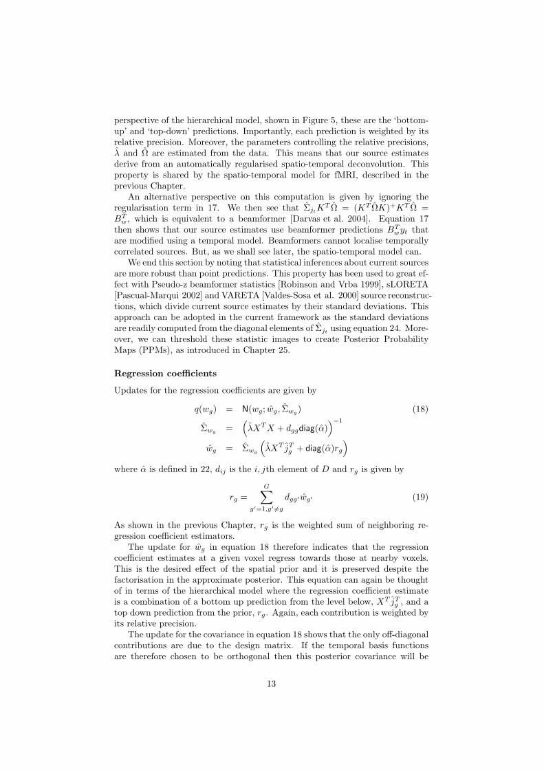
perspective of the hierarchical model, shown in Figure 5, these are the ‘bottom-up’ and ‘top-down’ predictions. Importantly, each prediction is weighted by itsrelative precision. Moreover, the parameters controlling the relative precisions,λ and Ω are estimated from the data. This means that our source estimatesderive from an automatically regularised spatio-temporal deconvolution. Thisproperty is shared by the spatio-temporal model for fMRI, described in theprevious Chapter.

An alternative perspective on this computation is given by ignoring theregularisation term in 17. We then see that ΣjtK

T Ω = (KT ΩK)+KT Ω =BT

w , which is equivalent to a beamformer [Darvas et al. 2004]. Equation 17then shows that our source estimates use beamformer predictions BT

wyt thatare modified using a temporal model. Beamformers cannot localise temporallycorrelated sources. But, as we shall see later, the spatio-temporal model can.

We end this section by noting that statistical inferences about current sourcesare more robust than point predictions. This property has been used to great ef-fect with Pseudo-z beamformer statistics [Robinson and Vrba 1999], sLORETA[Pascual-Marqui 2002] and VARETA [Valdes-Sosa et al. 2000] source reconstruc-tions, which divide current source estimates by their standard deviations. Thisapproach can be adopted in the current framework as the standard deviationsare readily computed from the diagonal elements of Σjt

using equation 24. More-over, we can threshold these statistic images to create Posterior ProbabilityMaps (PPMs), as introduced in Chapter 25.

Regression coefficients

Updates for the regression coefficients are given by

q(wg) = N(wg; wg, Σwg ) (18)

Σwg=

(λXT X + dggdiag(α)

)−1

wg = Σwg

(λXT jT

g + diag(α)rg

)where α is defined in 22, dij is the i, jth element of D and rg is given by

rg =G∑

g′=1,g′ 6=g

dgg′wg′ (19)

As shown in the previous Chapter, rg is the weighted sum of neighboring re-gression coefficient estimators.

The update for wg in equation 18 therefore indicates that the regressioncoefficient estimates at a given voxel regress towards those at nearby voxels.This is the desired effect of the spatial prior and it is preserved despite thefactorisation in the approximate posterior. This equation can again be thoughtof in terms of the hierarchical model where the regression coefficient estimateis a combination of a bottom up prediction from the level below, XT jT

g , and atop down prediction from the prior, rg. Again, each contribution is weighted byits relative precision.

The update for the covariance in equation 18 shows that the only off-diagonalcontributions are due to the design matrix. If the temporal basis functionsare therefore chosen to be orthogonal then this posterior covariance will be

13

diagonal, thus making a potentially large saving of computer memory. Onebenefit of the proposed framework, however, is that non-orthogonal bases canbe accomodated. This may allow for a more natural and compact descriptionof the data.

Precision of temporal models

Updates for the precision of the temporal model are given by

q(λ) = Ga(λ; bλpost , cλpost) (20)

1bλpost

=1

bλprior

+12

∑t

(||jt − WT xT

t ||2 + Tr(Σjt) +

G∑g=1

xtΣwgxT

t

)

cλpost= cλprior

+GT

2λ = bλpostcλpost

In the context of ERP analysis, these expressions amount to an estimate of thevariance of spontaneous activity in source space, λ−1, given by the squared errorbetween the ERP estimate, WT xT

t , and source estimate, jt, averaged over timeand space and the other approximate posteriors.

Precision of forward model

Updates for the precision of the sensor noise are given by

q(σ) = =M∏

m=1

q(σm) (21)

q(σm) = Ga(σm; bσpost, cσpost

)1

bm=

1bσprior

+12

∑t

(ymt − kT

mjt

)2

+12kT

mΣjtkm

cm = cσprior +T

2σm = bmcm

Ω−1 = diag(σ)

These expressions amount to an estimate of observation noise at the mth sensor,σm

−1, given by the squared error between the forward model and sensor data,averaged over time and the other approximate posteriors.

14

Precision of spatial prior

Updates for the precision of the spatial prior are given by

q(α) =K∏

k=1

q(αk) (22)

q(αk) = Ga(αk; bαpost , cαpost)

1bαpost

=1

bαprior

+ ||DwTk ||2 +

G∑g=1

dgsgk

cαpost= cαprior

+G

2αk = bαpostcαpost

where sgk is the kth diagonal element of Σwg . These expressions amount to anestimate of the ‘spatial noise variance’, α−1

k , given by the discrepancy betweenneighboring regression coefficients, averaged over space and the other approxi-mate posteriors.

Implementation details

A practical difficulty with the update equations for the sources is that the co-variance matrix Σjt

is of dimension G × G where G is the number of sources.Even low resolution source grids typically contain G > 1000 elements. Thistherefore presents a problem. A solution is found, however, with use of a Sin-gular Value Decomposition (SVD). First, we define a modified lead field matrixK = Ω1/2K and compute its SVD

K = USV T (23)= UV

where V is an M × G matrix, the same dimension as the lead field, K. It canthen be shown using the matrix inversion lemma [Golub and Van Loan 1996]that

Σjt= λ−1 (IG −RG) (24)

RG = V T (λIM + SST )−1V

which is simple to implement computationally, as it only requires inversion ofan M ×M matrix.

Source estimates can be computed as shown in equation 17. In principle,this means the estimated sources over all time points and source locations aregiven by

J = ΣjtKT ΩY + λΣjt

WT XT

In practice, however, it is inefficient to work with such a large matrix duringestimation. We therefore do not implement equations 16 and 17 but, instead,work in the reduced space JX = JX which are the sources projected onto the

15

design matrix. These projected source estimates are given by

JX = JX (25)

= ΣjtKT ΩY X + λΣjt

WT XT X

= AKΩY X + λAW XT X

where Y X and XT X can be pre-computed and the intermediate quantities aregiven by

AKΩ = ΣjtKT Ω (26)

= λ−1(KT −RGKT

)AW = ΣjtW

T

= λ−1(WT −RGWT

)Because these matrices are only of dimension G ×M and G ×K respectively,JX can be efficiently computed. The term XT jT

g in equation 18 is then givenby the gth row of JX .

The intermediate quantities can also be used to compute model predictionsas

Y = KJ (27)

= KAKΩY + λKAW XT

The m, tth entry in Y then corresponds to the kTmjt term in equation 21. Other

computational savings are as follows. For equation 21 we use the result

kTmΣjt

km =1

σm

M∑m′=1

s2m′m′u2

mm′

s2m′m′ + λ

(28)

where sij and uij are the i, jth entries in S and U respectively. For equation 20we use the result

Tr(Σjt) =

M∑i=1

1

s2ii + λ

+G−M

λ(29)

To summarise, our source reconstruction model is fitted to data by iterativelyapplying the update equations until the change in the negative free energy (seeChapter 26), F , is less than some user-specified tolerance. This procedure issummarised in the pseudo-code in Figure 6. This amounts to a process in whichsensor data is spatially deconvolved, time series models are fitted in sourcespace, and then the precisions (accuracy) of the temporal and spatial modelsare estimated. This process is then iterated and results in a spatio-temporaldeconvolution in which all aspects of the model are optimised to maximise alower bound on the model evidence.

Results

This section presents some preliminary qualitative results. In what follows werefer to the spatio-temporal approach as ‘VB-GLM’.

16

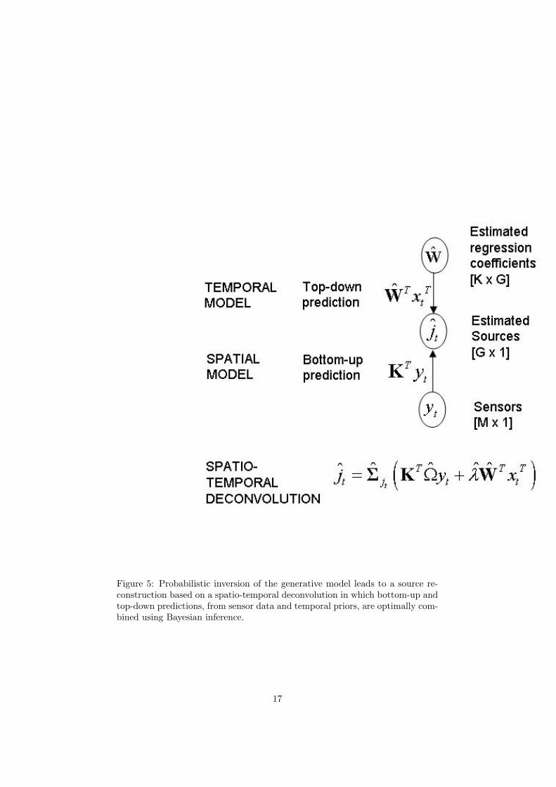
Figure 5: Probabilistic inversion of the generative model leads to a source re-construction based on a spatio-temporal deconvolution in which bottom-up andtop-down predictions, from sensor data and temporal priors, are optimally com-bined using Bayesian inference.

17

Figure 6: Pseudo code for spatio-temporal deconvolution of M/EEG. The pa-rameters of the model θ = J,W,Ω, λ, α are estimated by updating the approx-imate posteriors until the negative free energy is maximised to within a certaintolerance (left panel). At this point, because the log evidence L = log p(Y ) isfixed, the approximate posteriors will best approximate the true posteriors inthe sense of KL-divergence (right panel), as described in Chapter 26. The equa-tions for updating the approximate posteriors are given in the theory section.

18

Comparison with LORETA

We generated data from our model as follows. Firstly, we created two regressorsconsisting of a 10 Hz and 20Hz sinewave with amplitudes of 10 and 8 respectively.These formed the two columns of a design matrix shown in Figure 7. Wegenerated 600ms of activity with a sample period of 5ms, giving 120 time points.

The sensor space was defined using M = 32 electrodes from the Brain Elec-trical Source Activity (BESA) system [Scherg and von Cramon 1986] shown inFigure 8. We used the three concentric sphere model to calculate the electriclead field [Rush and Driscoll 1969]. The center and radius of the spheres werefitted to the scalp, skull and cerebral tissue of a ‘typical’ brain from the Mon-treal Neurological Institute (MNI) data base [Evans et al. 1993]. The sourcespace consisted of a mesh of points corresponding to the vertices of the trianglesobtained by tessellation of the cortical surface of the same brain. A mediumresolution spatial grid was used containing G = 10, 242 points.

We define the Signal to Noise Ratio (SNR) as the ratio of the signal standarddeviation to noise standard deviation and used sensor and source SNRs of 10and 40 respectively. The spatial distribution of the two regression coefficientswere identical, each of them consisting of two Gaussian blobs with a maximumamplitude of 10, and a Full Width at Half Maximum (FWHM) of 20mm.

Figure 9 shows the true and estimated sources at time point t = 20ms.The LORETA solution was found from an instantaneous reconstruction of thesensor data at that time point, using an L2-norm and a spatial regularisationparameter α (see equation 1) estimated using generalised cross-validation. TheVB-GLM solution was found by applying the VB update equations described inthe Theory section. As expected, VB provides a better solution both in termsof localisation accuracy and scaling.

ERP simulation

We then used our generative model to simulate ERP-like activity by using theregressors shown in Figure 10. The first regressor mimics an early componentand the second a later component. These regressors were derived from a neu-ral mass model describing activity in a distributed network of cortical areas[David and Friston 2003], which lends these simulations a degree of biologicalplausibility. These neural mass models are described at length in Chapter 32.

We then specified two source activations with the same amplitude and FWHMas in the previous example. The source space, sensor space and forward modelwere also identical to the previous example. Ten trials of sensor data were thengenerated using the same SNR as in the previous set of simulations. Signalepochs of 512ms were produced with a sampling period of 4ms giving a total of5120ms of EEG. The data were then averaged over trials to calculate the sampleERP shown in Figure 11.

We then estimated the sources underlying the sample ERP with (i) a cor-rectly specified model using the same two regressors used for generating the dataand (ii) an over-specified model that also incorporated two additional spuriousregressors shown in Figure 12. The design matrices for each of these models areshown in Figure 13. In the over-specified model, regressors 2 and 3 are highlycorrelated (r = 0.86). This can be seen most clearly in Figure 13.

The models were then fitted to the data using the VB update rules. As

19

Figure 7: Simulations that compare VB-GLM with LORETA used the abovedesign matrix, X. The columns in this matrix comprise a 10Hz and a 20Hzsinewave.

20

Figure 8: Electrode positions for the 32-sensor BESA system (left) and 128-sensor BioSemi system (right).

21

Figure 9: True and estimated source distributions at time t = 20ms. Note thescaling in the figures. The VB-GLM approach is better both in terms of spatiallocalisation and the scaling of source estimates.

22

Figure 10: Two ERP components, derived from a biophysical model, used togenerate simulated ERP data. These mimic an early component and a latecomponent.

23

Figure 11: A butterfly plot of simulated ERPs at 32 sensors.

24

Figure 12: Four components, derived from a biophysical model, used in anover-specified ERP model.

25

Figure 13: Design matrices, X, used for localisation of biophysical components.Model 1 (left) contains the regressors used to generate the data and Model 2(right) contains two additional spurious regressors. These regressors have beenplotted as time series in Figures 10 and 12.

26

Figure 14: Regression coefficients, wg, from ERP simulation. ’Coeff 1’ and’Coeff 2’ denote the first and second entries in the regression coefficient vectorwg. True model (left) and estimates from correctly specified model (right).

27

Figure 15: Estimated regression coefficients, wg, from over-specified model. Thetrue coefficients are shown in Figure 14. Note the scaling of coefficients 3 and4 (the true values are zero). Despite the high temporal correlation betweenregressors 2 and 3, the coefficients for regressor 3 have been correctly shrunktowards zero. This is a consequence of the spatial prior and the iterative natureof the spatio-temporal deconvolution (see Figure 6).

28

Figure 16: True regression coefficients for ERP simulation with correlatedsources. This simulation used a design matrix comprising the regressors shownin Figure 12, with the first and fourth coefficients set to zero and the secondand third set as shown in this figure.

29

Figure 17: Estimated regression coefficents, wg, for ERP simulation with corre-lated sources. Coefficients 2 and 3 resemble the true values shown in Figure 16whereas regressors 1 and 4 have been correctly shrunk towards zero by thespatio-temporal deconvolution algorithm.

30

shown in Figures 14 and 15, the true effects (regression coefficients) are ac-curately recovered even for the over-specified model. The spurious regressioncoefficients are shrunk towards zero. This is a consequence of the spatial priorand the iterative spatio-temporal deconvolution. This also shows that sourcereconstruction with temporal priors is robust to model mis-specification.

We then performed a second simulation with the set of regressors shown inFigure 12, and identical specifications of source space, sensor space, forwardmodel and SNR. But in this example we generated data from the regressioncoefficients shown in Figure 16, regression coefficients one and four being setto zero. This data therefore comprises three distributed sources (i) a right-lateralised source having time series given by a scaled, noise-corrupted regressor2, (ii) a frontal source given by a scaled, noise-corrupted regressor 3 and (iii) aleft-lateralised source comprising a noisy, scaled mixture of regressors 2 and 3.These sources are therefore highly correlated.

The VB-GLM model, using a full design matrix comprising all four regres-sors, was then fitted to this data. The estimated regression coefficients areshown in Figure 17. Regressors 1 and 4 have been correctly estimated to beclose to zero whereas regressors 2 and 3 bear a close resemblance to the truevalues. This shows that VB-GLM, in contrast to eg. beamforming approaches,is capable of localising temporally correlated sources.

Face ERPs

This section presents an analysis of a face processing EEG data set from Hensonet al. [Henson et al. 2003]. The experiment involved presentation of images offaces and scrambled faces, as described in Figure 18.

The EEG data were acquired on a 128-channel BioSemi ActiveTwo system,sampled at 1024 Hz. The data were referenced to the average of left and rightearlobe electrodes and epoched from -200ms to +600ms. These epochs werethen examined for artifacts, defined as timepoints that exceeded an absolutethreshold of 120 microvolts. A total of 29 of the 172 trials were rejected. Theepochs were then averaged to produce condition specific ERPs at each electrode.

The first clear difference between faces and scrambled faces is maximalaround 160ms, appearing as an enhancement of a negative component (peak’N160’) at occipito-temporal channels (eg. channel ‘B8’), or enhancement of apositive peak at Cz (eg channel ‘A1’). These effects are shown as a differentialtopography in Figure 19 and as time series in Figure 20.

A temporal model was then fitted using wavelet shrinkage [Donoho and Johnstone 1994].Before applying the model, the data were first downsampled and the 128 sam-ples following stimulus onset were extracted. These steps were taken as we usedWaveLab 1 to generate the wavelet bases. This uses a pyramid algorithm tocompute coefficients, so requiring the number of samples to be a power of two.

We then extracted the first eigenvector of the sensor data using a SingularValue Decomposition (SVD) and fitted wavelet models to this time series. Anumber of wavelet bases were examined, two samples of which are shown inFigure 4 . These are the Daubechies-4 and Battle-Lemarie-3 wavelets. Figure 21shows the corresponding time series estimates. These employed K = 28 andK = 23 basis functions respectively, as determined by application of the wavelet

1WaveLab is available from http://www-stat.stanford.edu/wavelab.

31

shrinkage algorithm [Donoho and Johnstone 1994]. We used the smaller Battle-Lemarie basis set in the source reconstruction that follows.

ERPs for faces and scrambled faces were then concatenated to form a vectorof 256 elements at each electrode. The overall sensor matrix Y was then ofdimension 256 × 128. The design matrix, of dimension 256 × 46, was createdby having identical block diagonal elements each comprising the Battle-Lemariebasis. This is shown in Figure 22. The source space was then defined using amedium resolution cortical grid defined using the typical MNI brain, as in theprevious sections. Current source orientations were assumed perpendicular tothe cortical surface. Constraining current sources based on a different individ-uals anatomy is clearly sub-optimal, but nevertheless allows us to report somequalitative results.

We then applied the source reconstruction algorithm and obtained a solutionafter twenty minutes of processing. Figure 23 shows differences in the sourceestimates for faces minus scrambled faces at time t = 160ms. The images showdifferences in absolute current at each voxel. They have been thresholded at50% of the maximum difference at this time point. The maximum difference isplotted in red and 50% of the maximum difference in blue. At this thresholdfour main clusters of activation appear at (i) right fusiform, (ii) right anteriortemporal, (iii) frontal and (iv) superior centro-parietal.

These activations are consistent with previous fMRI [Henson et al. 2003]and MEG analyses of faces minus scrambled faces in that face processing islateralised to the right hemisphere and in particular to fusiform cortex. Addi-tionally, the activations in temporal and frontal regions, although not signifi-cant in group random effects analyses, are nonetheless compatible with observedbetween- subject variability on this task.

Discussion

This Chapter has described a model-based spatio-temporal deconvolution ap-proach to source reconstruction. Sources are reconstructed by inverting a for-ward model comprising a temporal process as well as a spatial process. Thisapproach relies on the fact that EEG and MEG signals are extended in time aswell as in space.

It rests on the notion that MEG and EEG reflect the neuronal activityof a spatially distributed dynamical system. Depending on the nature of theexperimental task, this activity can be highly localised or highly distributedand the dynamics can be more, or less, complex. At one extreme, listening forexample to simple auditory stimuli produces brain activations that are highlylocalised in time and space. This activity is well described by a single dipolelocated in brainstem and reflecting a single burst of neuronal activity at eg.t=20ms post-stimulus. More complicated tasks, such as oddball paradigms,elicit spatially distributed responses and more complicated dynamics that canappear in the ERP as damped sinusoidal responses. In this Chapter we havetaken the view that by explictly modelling these dynamics one can obtain bettersource reconstructions.

This view is not unique within the source reconstruction community. In-deed, there have been a number of approaches that also make use of temporalpriors. Baillet and Garnero [Baillet and Garnero 1997], in addition to consid-

32

ering edge-preserving spatial priors, have proposed temporal priors that pe-nalise quadratic differences between neighboring time points. Schmidt et al.[Schmidt et al. 2000] have extended their dipole-like modelling approach usinga temporal correlation prior which encourages activity at neighboring latenciesto be correlated. Galka et al. [Galka et al. 2004] have proposed a spatiotempo-ral Kalman filtering approach which is implemented using linear autoregressivemodels with neighborhood relations. This work has been extended by Yamashitaet al. [Yamashita et al. 2004] who have developed a ‘Dynamic LORETA’ algo-rithm in which the Kalman filtering step is approximated using a recursivepenalised least squares solution. The algorithm is, however, computationallycostly, taking several hours to estimate sources in even low-resolution sourcespaces.

Compared to these approaches, our algorithm perhaps embodies strongerdynamic constraints. But the computational simplicity of fitting GLMs, alliedto the efficiency of variational inference, results in a relatively fast algorithm.Also, the GLM can accomodate damped sinusoidal and wavelet approaches thatare ideal for modelling transient and nonstationary responses.

The dynamic constraints implicit in our model help to regularize the solution.Indeed, with M sensors, G sources, T time points and K temporal regressorsused to model an ERP, if K < MT/G the inverse problem is no longer under-determined. In practice, however, spatial regularisation will still be required toimprove estimation accuracy.

This paper has described a spatio-temporal source reconstruction methodembodying well known phenomenological descriptions of ERPs. A similar methodhas recently been proposed in [Friston et al. 2006] (see also Chapter 30), but theapproaches are different in a number of respects. First, in [Friston et al. 2006]scalp data Y are (effectively) projected onto a temporal basis set X and sourcereconstructions are made in this reduced space. This results in a computation-ally efficient procedure based on Restricted Maximum Likelihood (ReML), butone in which the fit of the temporal model is not taken into account. This willresult in inferences about W and J which are over-confident. If one is simplyinterested in population inferences based on summary statistics (ie. W ) from agroup of subjects, then this does not matter. If, however, one wishes to makewithin-subject inferences then the procedure described in this chapter is the pre-ferred approach. Second, in [Friston et al. 2006] the model has been augmentedto account for trial-specific responses. This treats each trial as a ‘random effect’and provides a method for making inferences about induced responses. Thealgorithm described in this chapter, however, is restricted to treating trials asfixed effects. This mirrors standard first-level analyses of fMRI in which multipletrials are treated by forming concatenated data and design matrices.

A further exciting recent development in source reconstruction is the applica-tion of Dynamic Causal Models (DCMs) to M/EEG. DCMs can also be viewedas providing spatio-temporal reconstructions, but ones where the temporal pri-ors are imposed by biologically informed neural mass models. This offers thepossibility of making inferences about task-specific changes in the synaptic ef-ficacy of long range connections in cortical hierarchies, directly from imagingdata. These developments are described in Chapter 43.

33

References

[Auranen et al. 2005] T. Auranen, A. Nummenmaa, M. Hammalainen,I. Jaaskelainen, J. Lampinen, A. Vehtari, and M. Sams. Bayesian analysisof the neuromagnetic inverse problem with lp norm priors. Neuroimage26(3),870–884, 2005.

[Baillet and Garnero 1997] S. Baillet and L. Garnero. A Bayesian approach tointroducing anatomo-functional priors in the EEG/MEG inverse problem.IEEE Transactions on Biomedical Engineering, pages 374–385, 1997.

[Baillet et al. 2001] S. Baillet, J.C. Mosher, and R.M. Leahy. ElectromagneticBrain Mapping. IEEE Signal Processing Magazine, pages 14–30, November2001.

[Tallon-Baudry et al. 1996] C. Tallon Baudry, O. Bertrand, C. Delpuech, andJ. Pernier. Stimulus specificity of phase-locked and non phase-locked 40hzvisual responses in human. The Journal of Neuroscience, 16(13):4240–4249,1996.

[Breakspear and Terry 2002] M. Breakspear and J.R. Terry. Nonlinear inter-dependence in neural systems: motivation, theory and relevance. Interna-tional Journal of Neuroscience, 112:1263–1284, 2002.

[Brookes et al. 2004] M. Brookes, A. Gibson, S. Hall, P. Furlong, G. Barnes,A. Hillebrand, K. Singh, I. Halliday, S. Francis, and P. Morris. A generallinear model for MEG beamformer imaging. Neuroimage, 23(3):936–946,2004.

[Clyde et al. 1998] M. Clyde, G. Parmigiani, and B. Vidakovic. Multiple shrink-age and subset selection in wavelets. Biometrika, 85:391–402, 1998.

[Darvas et al. 2004] F. Darvas, D. Pantazis, E. Kucukaltun Yildirim, andR. Leahy. Mapping human brain function with MEG and EEG: methodsand validation. Neuroimage, 2004.

[David and Friston 2003] O. David and K.J. Friston. A neural mass model forMEG/EEG: coupling and neuronal dynamics. NeuroImage, 20(3):1743–1755, 2003.

[Demiralp et al. 1998] T. Demiralp, A. Ademoglu, Y. Istefanopoulos, and H.O.Gulcur. Analysis of event-related potentials (ERP) by damped sinusoids.Biological Cybernetics, 78:487–493, 1998.

[Donoho and Johnstone 1994] D.L. Donoho and I.M. Johnstone. Ideal spatialadaptation by wavelet shrinkage. Biometrika, 81:425–455, 1994.

[Evans et al. 1993] A. Evans, D. Collins, S. Mills, E. Brown, R. Kelly, andT. Peters. 3d statistical neuroanatomical models from 305 mri volumes.Proc. IEEE Nuclear Science Symposium and Medical Imaging Conference,95:1813–1817, 1993.

[Frackowiak et al. 2003] R.S.J. Frackowiak, K.J. Friston, C. Frith, R. Dolan,C.J. Price, S. Zeki, J. Ashburner, and W.D. Penny. Human Brain Function.Academic Press, 2nd edition, 2003.

34

[Friston et al. 2000] K.J. Friston, A. Mechelli, R. Turner, and C.J. Price. Non-linear responses in fMRI: The Balloon model, Volterra kernels and otherhemodynamics. NeuroImage, 12:466–477, 2000.

[Friston et al. 2006] K.J. Friston, R.N.A. Henson, C. Phillips, and J. Mattout.Bayesian estimation of evoked and induced responses. Neuroimage, ac-cepted for publication, 2006.

[Fuchs et al. 1999] M. Fuchs, M. Wagner, T. Kohler, and H. Wischman. Linearand nonlinear current density reconstructions. Journal of Clinical Neuro-physiology, 16(3):267–295, 1999.

[Galka et al. 2004] A. Galka, O. Yamashita, T. Ozaki, R.Biscay, and P. Valdes-Sosa. A solution to the dynamical inverse problem of EEG generation usingspatiotemporal Kalman filtering. NeuroImage, 23(2):435–453, 2004.

[Gelman et al. 1995] A. Gelman, J.B. Carlin, H.S. Stern, and D.B. Rubin.Bayesian Data Analysis. Chapman and Hall, Boca Raton, 1995.

[Golub and Van Loan 1996] G.H. Golub and C.F. Van Loan. Matrix Computa-tions. John Hopkins University Press, 3rd edition, 1996.

[Henson et al. 2003] R.N.A. Henson, Y. Goshen-Gottstein, T. Ganel, L.J. Ot-ten, A. Quayle, and M.D. Rugg. Electrophysiological and hemodynamiccorrelates of face perception, recognition and priming. Cerebral Cortex,13:793–805, 2003.

[Kiebel and Friston 2004] S.J. Kiebel and K.J. Friston. Statistical ParametricMapping for Event-Related Potentials II: A Hierarchical Temporal Model.NeuroImage, 22(2):503–520, 2004.

[Makeig et al. 2002] S. Makeig, M. Westerfield, T.-P. Jung, S. Enghoff,J. Townsend, E. Courchesne, and T.J. Sejnowski. Dynamic brain sourcesof visual evoked responses. Science, 295:690–694, 2002.

[Pascual-Marqui et al. 1994] R. Pascual Marqui, C. Michel, and D. Lehman.Low resolution electromagnetic tomography: a new method for localizingelectrical activity of the brain. International Journal of Psychophysiology,pages 49–65, 1994.

[Pascual-Marqui 2002] R. Pascual Marqui. Standardized low resolution electro-magnetic tomography (sLORETA): technical details. Methods and Findingsin Experimental and Clinical Pharmacology, 24:5–12, 2002.

[Mattout et al. 2006] J. Mattout, C. Phillips, W.D. Penny, M. Rugg, and K.J.Friston. MEG source localisation under multiple constraints: an extendedBayesian framework. NeuroImage, 30(3):753, 2006.

[McKeown et al. 1998] M.J. McKeown, S. Makeig, G.G. Brown, T.P. Jung, S.S.Kindermann, A.J. Bell, and T.J. Sejnowski. Analysis of fMRI data by blindseparation into independent spatial components. Human Brain Mapping,6:160–188, 1998.

35

[Minka 2000] T.P. Minka. Automatic choice of dimensionality for PCA. Tech-nical Report 514, MIT Media Laboratory, Perceptual Computing Section,2000.

[Mosher and Leahy 1998] J.C. Mosher and R.M. Leahy. Recursive MUSIC: aframework for eeg and meg source localization. IEEE Transactions onBiomedical Engineering, 47:332–340, 1998.

[Osborne and Smyth 1991] M.R. Osborne and G. K. Smyth. A modified Pronyalgorithm for fitting functions defined by difference equations. Journal ofScientific and Statistical Computing, 12:362–382, 1991.

[Penny and Flandin 2005] W.D. Penny and G. Flandin. Bayesian analysis ofsingle-subject fMRI: SPM implementation. Technical report, WellcomeDepartment of Imaging Neuroscience, 2005.

[Penny et al. 2005] W.D. Penny, N. Trujillo-Barreto, and K.J. Friston. BayesianfMRI time series analysis with spatial priors. NeuroImage, 24(2):350–362,2005.

[Roberts and Penny 2002] S.J. Roberts and W.D. Penny. Variational Bayes forGeneralised Autoregressive models. IEEE Transactions on Signal Process-ing, 50(9):2245–2257, 2002.

[Robinson and Vrba 1999] S. Robinson and J. Vrba. Functional neuroimagingby Synthetic Aperture Magnetometry (SAM). In Recent Advances in Bio-magnetism, Sendai, Japan, 1999. Tohoku University Press.

[Rugg and Coles 1995] M.D. Rugg and M.G.H. Coles. Electrophysiology ofMind: Event-Related Potentials and Cognition. Oxford University Press,1995.

[Rush and Driscoll 1969] S. Rush and D. Driscoll. EEG electrode sensitivity –an application of reciprocity. IEEE Transactions on Biomedical Engineer-ing, 16(1):15–22, 1969.

[Sahani and Nagarajan 2004] M. Sahani and S.S. Nagarajan. Reconstruct-ing MEG sources with unknown correlations. In L. Saul S. Thrun andB. Schoelkopf, editors, Advances in Neural Information Processing Sys-tems, volume 16. MIT, Cambridge, MA, 2004.

[Scherg and von Cramon 1986] M. Scherg and D. von Cramon. Evoked dipolesource potentials of the human auditory cortex. Electroencephalography andClinical Neurophysiology, 65:344–360, 1986.

[Schmidt et al. 1999] D.M. Schmidt, J.S. George, and C.C. Wood. Bayesianinference applied to the electromagnetic inverse problem. Human BrainMapping, 7:195–212, 1999.

[Schmidt et al. 2000] D.M. Schmidt, D.M. Ranken J.S. George, and C.C. Wood.Spatial-temporal Bayesian inference for MEG/EEG. In 12th InternationalConference on Biomagnetism, Helsink, Finland, August 2000.

36

[Trejo and Shensa 1999] L. Trejo and M.J. Shensa. Feature extraction of event-related potentials using wavelets: an application to human performancemonitoring. Brain and Language, 66:89–107, 1999.

[Unser and Aldroubi 1996] M. Unser and A. Aldroubi. A review of wavelets inbiomedical applications. Proceedings of the IEEE, 84:626–638, 1996.

[Valdes-Sosa et al. 2000] P. Valdes-Sosa, F. Marti, F. Garcia, and R. Casanova.Variable Resolution Electric-Magnetic Tomography. In Proceedings of the10th International Conference on Biomagnetism, volume 2, pages 373–376,2000.

[Woolrich et al. 2001] M.W. Woolrich, B.D. Ripley, M. Brady, and S.M. Smith.Temporal autocorrelation in univariate linear modelling of fMRI data. Neu-roImage, 14(6):1370–1386, December 2001.

[Yamashita et al. 2004] O. Yamashita, A. Galka, T. Ozaki, R. Biscay, andP. Valdes-Sosa. Recursive penalised least squares solution for dynamicalinverse problems of EEG generation. Human Brain Mapping, (21):221–235, 2004.

37

Figure 18: Face paradigm. The experiment involved randomised presentationof images of 86 faces and 86 scrambled faces. Half of the faces belong to fa-mous people, half are novel, creating 3 conditions in total. In this Chapterwe consider just two conditions (i) faces (famous or not) and (ii) scrambledfaces. The scrambled faces were created by 2D Fourier transformation, randomphase permutation, inverse transformation and outline-masking. Thus facesand scrambled faces are closely matched for low-level visual properties such asspatial frequency. The subject judged the left-right symmetry of each imagearound an imaginary vertical line through the centre of the image. Faces werepresented for 600ms, every 3600ms.

38

Figure 19: The figure shows differential EEG topography for faces minus scram-bled faces at t = 160ms poststimulus.

39

Figure 20: Sensor time courses for face data at occipito-temporal electrode B8(left) and vertex A1 (right) for faces (blue) and scrambled faces (red).

40

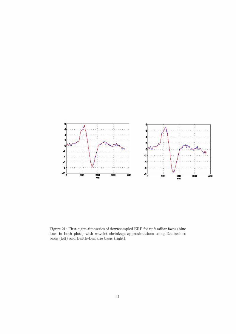
Figure 21: First eigen-timeseries of downsampled ERP for unfamiliar faces (bluelines in both plots) with wavelet shrinkage approximations using Daubechiesbasis (left) and Battle-Lemarie basis (right).

41

Figure 22: Design matrix for source reconstruction of ERPs from Face data.Each block contains a 23-element Batte-Lemarie basis set. The first components,forming diagonals in the picture, are low frequency wavelets. The high frequencywavelets are concentrated around the N160, where the signal is changing mostquickly.

42

Figure 23: These images are derived from the source reconstruction of ERPsin response to faces and scrambled faces. The plots show absolute differencesbetween faces and scrambled faces at t=160ms post-stimulus. The maps havebeen thresholded such that the largest difference appears in red and 50% of thelargest difference appears in blue.

43