Embed Size (px)
Citation preview
CHAPTER 2
APPROXII\/IATION AND INTERPOLATION
The present chapter is basically concerned with the approximation of functions. The functions in question may be functions defined on a contin- uum - typically a finite interval - or functions defined only on a finite set of points. The first instance arises, for example, in the context of special functions (elementary or transcendental) that one wishes to evaluate as part of a subroutine. Since any such evaluation must be reduced to a finite num- ber of arithmetic operations, we must ultimately approximate the function by means of a polynomial or a rational function. The second instance is fre- quently encountered in the physical sciences when measurements are taken of a certain physical quantity as a function of some other physical quantity (such as time). In either case one wants to approximate the given function "as well as possible" in terms of other simpler functions.
The general scheme of approximation can be described as follows. We are given the function f to be approximated, along with a class @ of "approx- imating functions" cp and a "normi' ( 1 . I( measuring the overall magnitude of functions. We are looking for an approximation $ E @ of f such that
The function $ is called the best approximation to f from the class @, relative to the norm 1 ) - 1 1 .
The class @ is called a (real) linear space if with any two functions cp l ,
cpz E @ it also contains cpl + and ccpl for any c E R, hence also any (finite) linear combination of functions cpi E @. Given n "basis functions" .rrj E @, j = 1 , 2 , . . . , n, we can define a linear space of finite dimension n by
@ = @ n = { ( ~ : q( t ) = C c j x j ( t ) , ~j E R). j=1
(0.2)
Examples of linear spaces @
(1) @ = P,: polynomials of degree 5 m. A basis for P, is; for example, x 3 (t) = tj-', j = 1,2, . . . , m+ 1, so that n = m+ 1. Polynomials,are the most frequently used "general-purpose" approximants for dealing with functions on bounded domains (finite intervals or finite sets of points). One reason
5 6 Chapter 2. Approximation and Interpolation
is Weierstrass's theorem, which states that. any continuous function can be approximated on a finite interval as closely as one wishes by a polynomial of sufficiently high degree.
(2) @ = s ~ ( A ) : (polynomial) spline functions of degree m and smooth- ness class k on the subdivision
of the interval [a, b]. These are piecewise polynomials of degree 5 m pieced together at the "joints" t2 , . . . , t ~ - l in such a way that all derivatives up to and including the kth are continuous on the whole interval [a, b], including the joints:
We assume here 0 5 k < m; otherwise, we are back to polynomials IP, (see Ex. 62). We set k = -1 if we allow discontinuities at the joints. The dimension of s ~ ( A ) is n = (m - k) . ( N - 2) + m + 1 (see Ex. 65), but to find a basis is a nontrivial task; for m = 1, see $3.2.
(3) @ = T, [0,2.i.r]: trigonometric polynomials of degree 5 m on [O, 2 ~ 1 . These are linear combinations of the basic harmonics up to and including the mth one, that is,
.i.rk(t) = cos (k - l ) t , k = 1 , 2 , . . . , m + 1;
~ , + ~ + k ( t ) = sin kt, k = 1 , 2 , . . . , m,
where now n = 2m + 1. Such approximants are a natural choice when the function f to be approximated is periodic with period 27r. (If f has period p, one makes a preliminary change of variables t t . p/27r.)
(4) @ = En: exponential sums. For given distinct aj > 0, one takes Tj(t) = e - ~ j t , j = 1 ,2 , . . . , n. Exponential sums are often employed on the half-infinite interval R+: 0 5 t < oo, especially if one knows that f decays exponentially as t -+ co.
Note that the important class of rational functions,
is not a linear space. (Why not?)
Chapter 2. Approximation and Interpolation 57
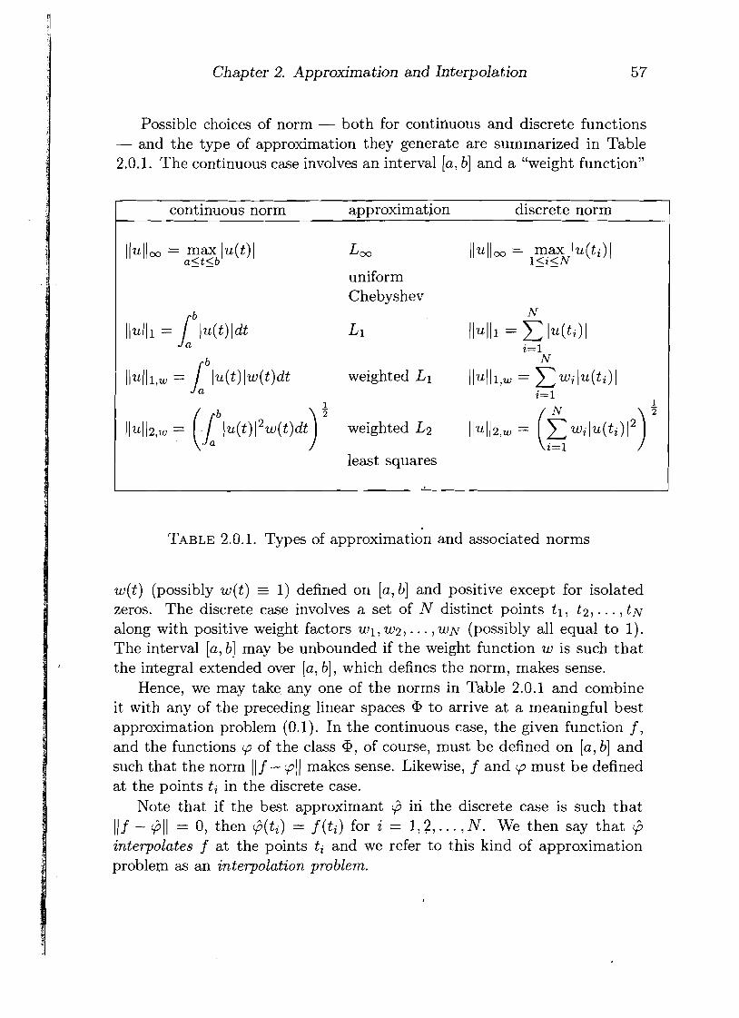
Possible choices of norm - both for contifiuous and discrete functions - and the type of approximation they generate are summarized in Table 2.0.1. The continuous case involves an interval [a, b] and a "weight function"
continuous norm approximation discrete norm
= max Ju( t )J I I u l l r n a<t<b
uniform Chebyshev
b N
ll~lll = l ~ ( t ) l d t L1 ll~II1 = C I ~ ( t i ) l i= 1
b N
IIuII1,w = Jd Iu(t)Iw(t)dt weighted L1 / / ~ ( I l , w = C ~ i I ~ ( t i ) l i= 1
1 - 1 2
weighted L2
least squares
TABLE 2.0.1. Types of approximation and associated norms
w(t) (possibly w(t) = 1) defined on [a, b] and positive except for isolated zeros. The discrete case involves a set of N distinct points t l , t2, . . . , t~ along with positive weight factors wl, w2, . . . , WN (possibly all equal to 1). The interval [a, b] may be unbounded if the weight function w is such that the integral extended over [a, b], which defines the norm, makes sense.
Hence, we may take any one of the norms in Table 2.0.1 and combine it with any of the preceding linear spaces to arrive at a meaningful best approximation problem (0.1). In the continuous case, the given function f , and the functions cp of the class a, of course, must be defined on [a, b] and such that the norm 1 1 f - cp 1 1 makes sense. Likewise, f and cp must be defined at the points ti in the discrete case.
Note that if the best approximant @ in the discrete case is such that J J f - $ 1 1 = 0, then @(ti) = f ( t i ) for i = I , ? , . . . , N. We then say that $3 interpolates f at the points ti and we refer to this kind of approximation problem as an interpolation problem.
Chapter 2. Approximation and Interpolation
The simplest approximation problems are the least squares problem and the interpolation problem, and the easiest space Qi to work with the space of polynomials of given degree. These are indeed the problems we concentrate on in this chapter. In the case of the least squares problem, however, we admit general linear spaces Qi of approximants, and also in the case of the interpolation probIem, we include polynomial splines in addition to straight polynomials.
Before we start with the least squares problem, we introduce a nota- tional device that allows us to treat the continuous and the discrete case simultaneously. We define, in the continuous case,
( 0 if t < a (whenever - ca < a),
Then we can write, for any (say, continuous) function u,
since dX(t) = 0 iLoutside" [a, b], and dX(t) = w(t)dt inside. We call dX a continuous (positive) measure. The discrete measure (also called "Dirac measure") associated with the point set I t l , t:!, . . . , t ~ ) is a measure dX that is nonzero only at the points ti and has the value wi there. Thus, in this case,
,. N
(A more precise definition can be given in terms of Stieltjes integrals, if we define X(t) to be a step function having jump wi a t ti.) In particular, we can define the L2 norm as
and obtain the continuous or the discrete norm depending on whether X is taken to be as in (0.3), or a step function, as in (0.4').
We call the support of dX - and denote it by suppdX - the interval [a, b] in the continuous case (assuming w positive on [a, b] except for isolated
$ 1. Least Squares Approximation 59
zeros), and the set i t l , t2, . . . , tN) in the discrete case. We say that the set of functions r j ( t ) in (0.2) is linearly independent on the support of dX if
n x c j r j (t) 0 for all t E supp dX implies cl = cz = . = C, = 0. (0.6) j= 1
Example: The powers r j ( t ) = tj-', j = 1 ,2 , . . . , n. n
Here C cjrj(t) = pn-1(t) is a polynomial of degree 5 n - 1. Suppose, j=l
first, that supp dX = [a, b]. Then the identity in (0.6) says that pn-1 (t) - 0 on [a, b] . Clearly, this implies cl = c:! = . - . = c, = 0, so that the powers are linearly independent on supp dX = [a, b]. If, on the other hand, suppdX = {tl, t2,. . . , tN), then the premise in (0.6) says that pn_l(ti) = 0, i = 1,2 , . . . , N; that is, pn-1 has N distinct zeros ti. This implies pn-1 _= 0
N
only if N > n. Otherwise, pn-1 (t) = n ( t - ti) E h-1 would satisfy i= 1
pn-1 (ti) = 0, i = 1,2, . . . , N, without being identically zero. Thus, we have linear independence on supp dX = {t 1, t2, . . . ; tN} if and only if N >_ n.
$1. Least Squares Approximat ion
We specialize the best approximation problem (0.1) by taking as norm the L2 norm
where dX is either a continuous measure (cf. (0.3)) or a discrete measure (cf. (0.4')), and by using approximants cp from an n-dimensional linear space
Here the basis functions ?r, are assumed linearly independent on suppdX (cf. (0.6)). We furthermore assume, of course, that the integral in (1.1) is meaningful whenever u = rj or u = f , the given function to be approxi- mated.
60 Chapter 2. Approximation and Interpolation
The solution of the least squares problem is most easily expressed in terms of orthogonal systems .irj relative to an appropriate inner product. We therefore begin with a discussion of inner products.
51.1. Inner products. Given a continuous or discrete measure dX, as introduced earlier, 'and given any two functions u: u having a finite norm (1.1), we can define the inner product
(Schwarz's inequality [(u, u) 1 5 11u 1I2,dx . 1171 1I2,dx tells us that the integral in (1.3) is well defined.) The inner product (1.3) has the following obvious (but useful) properties.
(i) symmetry: (u? u) = (v, u),
(ii) homogeneity: (au, u) = a ( u , u), a E R,
(iii) additivity: (u + v, w) = (u, w) + (u, w), and
(iv) positive definiteness: (u, u) 2 0, with equality holding if and only if u r 0 on suppdX.
Homogeneity and additivity together give linearity,
in the first variable and, by symmetry, also in the second. Moreover, (1.4) easily extends to linear combinations of arbitrary finite length. Note also that
llull%d~ = ( ~ ~ 4 - (1.5)
We say that u and u are orthogonal if
(u, u) = 0. (1-6)
This is always trivially true if either u or v vanishes identically on supp dX. It is now a simple exercise, for example, to prove the Theorem of Pythago-
ras:
if (u, u ) = 0, then (lu + v(I2 = I ( u ( ( ~ + (lull2, (1.7)
fj 1.1. Inner products 61
where 1 1 . 1 ) = 1 1 . 1)2,dX. (From now on we use thisabbreviated notation for the norm.) Indeed,
llu + v1I2 = (u + v, u + v) = (u, U) + (u, v) + (v, U) + (v, v)
= 1Iu1l2 + 2(u, v) + llv1I2 = 1Iu1l2 + 1Iv1l2,
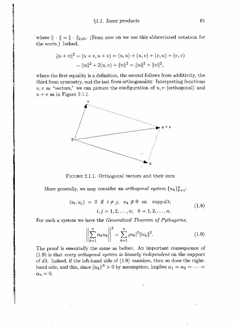
where the first equality is a definition, the second follows from additivity, the third from symmetry, and the last from orthogonality. Interpreting functions U, v as LLvectors," we can picture the configuration of u, v (orthogonal) and u + v as in Figure 2.1.1.
FIGURE 2.1.1. Orthogonal vectors and their sum
More generally, we may consider an orthogonal system { u ~ ) ; = ~ :
(ui, uj) = 0 if i # j, uk $ 0 on suppdX;
j = 1 , 2 , n k = 1,2 , . . . , n .
For such a system we have the Generalized Theorem of Pythagoras,
The proof is essentially the same as before. An important consequence of (1.9) is that every orthogonal system is linearly 'independent on the support of dX. Indeed, if the left-hand side of (1.9) vanishes, then so does the right- hand side, and this, since lluk 1 1 2 > 0 by assumption, implies a1 = a 2 = . . . =
an = 0.
62 Chapter 2. Approximation and Interpolation
81.2. The normal. -equations. We are now in a position to solve the least squares approximation problem. By (1.5), we can write the L2 error, or rather its square, in the form
Inserting p here from (1.2) gives
The squared L2 error, therefore, is a quadratic function of the coefficients cl, c2, . . . , C, of p. The problem of best L2 approximation thus amounts to minimizing a quadratic function of n variables. This is a standard problem of calculus and is solved by setting all partial derivatives equal to zero. This yields a system of linear algebraic equations. Indeed, differentiating partially with respect to c; under the integral sign in (1.10) gives
and setting this equal to zero, interchanging integration and summation in the process, we get
C (?Ti,rj)~j = (7iil f ) , i = 11 21. - . 1 n- (1.11) j=1
These are called the normal equations for the least squares problem. They form a linear system of the form
where the matrix A and the vector b have elements
A = [a,], aij = (xi, 71)); b = [bill bi = (r i , f ) . (1.11")
By symmetry of the inner product, A is a symmetric matrix. Moreover, A is positive definite; that is,
51.2. The normal equations 63
The quadratic function in (1.12) is called a quadratic form (since.it is homo- geneous of degree 2). Positive definiteness of A thus says that the quadratic form whose coefficients are the elements of A is always nonnegative, and zero only if all variables xi vanish.
To prove (1.12), all we have to do is insert the definition of the aij and use the elementary properties (i) through (iv) of the inner product:
n
This clearly is nonnegative. It is zero only if C xiri -- 0 on supp dX, which, i= 1
by the assumption of linear independence of the Ti, implies x l = x2 = . - =
xn = 0. Now it is a well-known fact of linear algebra that a symmetric positive
definite matrix A is nonsingular. Indeed, its determinant, as well as all its leading principal minor determinants, are strictly positive. It follows that the system (1.11) of normal equations has a unique solution. Does this so- lution correspond to a minimum of E[p] in (1.10)? Calculus tells us that for this to be the case, the Hessian matrix H = [a2E2/aciay] hag to be positive definite. But H = 2A, since is a quadratic function. Therefore, H, with A, is indeed positive definite, and the solution of the normal equations gives us the desired minimum. The least squares approximation problem thus has a unique solution, given by
where i. = [E l ,C2 , . . . , & I T is the solution vector of the normal equation (1.11).
This completely settles the least squares approximation problem in the- ory. How about in practice?
Assuming a general set of (linearly independent) basis functions, we can see the following possible difficulties.
(1) The system (1.11) may be ill-conditioned. A simple example is provided by supp dX = [0, 11, dX(t) = dt on [0,1], and rj (t) = t j - l , j = 1,2, . . . , n. Then
Chapter 2. Approximation and Interpolation
that is, the matrix A in (1.11) is precisely the Hilbert matrix. (Cf. Ch. 1, (341)) The resulting severe ill-conditioning of the normal equations in this example is entirely due to an unfortunate choice of basis functions - the powers. These become almost linearly dependent, more so the larger the exponent (cf. Ex. 35). Another source of degradation lies in the element bj = J' o 7i 3 ,(t) f (t)dt of the right-hand vector b in (1.11). When j is large, the power 7ij = tj-' behaves very much like a discontinuous function on [O,l.]: it is practically zero for much of the interval until it shoots up to the value 1 at the right endpoint. This has the unfortunate consequence that a good deal of information about f is lost when one forms the integral defining bj. A polynomial 7ij that oscillates rapidly on [0,1] would seem to be preferable from this point of view, since it would "engage" the function f more vigorously over all of the interval [0,1].
(2) The second disadvantage is the fact that all coefficients Ej in (1.13)
depend on n; that is, S = Ey), j = 1 ,2 , . . . , n. Increasing n, for example, will give an enlarged system of normal equations with a completely new solution vector. We refer to this as the n o n p e m a n e n c e of the coefficients A Cj.
Both defects (1) and (2) can'be eliminated (or at least attenuated in the case of (1)) in one stroke: select for the basis functions 7ij an orthogonal system,
(m , 7ij) = 0 if i # j ; (7ijl 7ij) = l/7ij 1 1 2 > 0. (1.14)
Then the system of normal equations becomes diagonal and is solved imme- diately by
Clearly, each of these coefficients ej is independent of n, and once computed, remains the same for any larger n. We now have permanence of the coeffi- cients. Also, we do not have to go through the trouble of solving a linear system of equations, but instead can use the formula (1.15) directly. This does not mean that there are no numerical problems associated with (1.15). Indeed, it is typical that the denominators l17ij ( I 2 in (1.15) decrease rapidly with increasing j, whereas the integrand in the numerator (or the individual terms in the case of a discrete inner product) are of the same magnitude as f . Yet the coefficients ej also, are expected to decrease rapidly. There- fore, cancellation errors must occur when one computes the inner product in the numerator. The cancellation problem can be alleviated somewhat by
3 1.3. Least squai-es error; convergence
computing Cj in the alternative form
where the empty sum (when j = 1) is taken to be zero, as usual. Clearly, by orthogonality of the rj, (1.15') is equivalent to (1.15) mathematically, but not necessarily numerically.
An algorithm for computing Zj from (1.15'), and at the same time $(t), is as follows:
so = 0, for j = 1,2, . . . , n do
This produces the coefficients tl, t2, . . . , & as well as $(t) = s,. Any system {irj) that is linearly independent on the support of dX can
be orthogonalized (with respect to the measure dX) by a device known as the Gram-Schmidt procedure. One takes
and, for j = 2,3, . . . , recursively forms
Then each rj so determined is orthogonal to all preceding ones.
$1.3. Least squares error; convergence. We have seen in 31.2 that if the class = a, consists of n functions rj, j = 1,2, . . . , n , that are linearly independent on the support of some measure dX, then the least squares problem for this measure,
has a unique solution @ = @, given by (1.13). There are many ways we can select a basis rj in a, and, therefore, many ways the solution @, can
Chapter 2. Approximation and Interpolation
be represented. Nevertheless, it is always one and the same function. The least squares error - the quantity on the right of (1.16) - therefore is independent of the choice of basis functions (although the calculation of the least squares solution, as mentioned previously, is not). In studying this error, we may thus assume, without restricting generality, that the basis rj is an orthogonal system. (Every linearly independent system can be orthogonalized by the Gram-Schmidt ort hogonalization procedure; cf. fj 1.2.) We then have (cf. (1.15))
We first note that the error f - Gn is orthogonal to the space an; that is,
(f - @,,cp) = 0 for all cp E a,, (1.18)
where the inner product is the one in (1.3). Since cp is a linear combination of the r k , it suffices to show (1.18) for each cp = r k , k = 1,2, . . . , n. Inserting @, from (1.17) in the left of (1.18), and using orthogonality, we find indeed
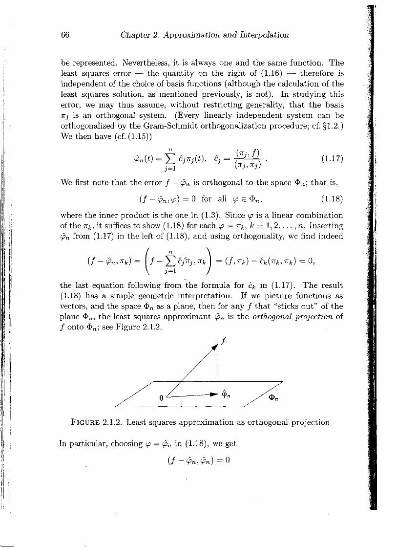
the last equation following from the formula for in (1.17). The result (1.18) has a simple geometric interpretation. If we picture functions as vectors, and the space an as a plane, then for any f that "sticks out" of the plane a,, the least squares approximant Gn is the orthogonal projection of f onto an; see Figure 2.1.2.
FIGURE 2.1.2. Least squares approximation as orthogonal projection
In particular, choosing cp = Gn in (.1.18), we get
fj 1.3. Least squares error; convergence 67
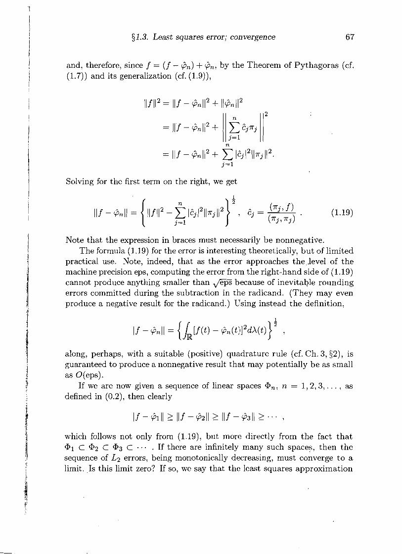
and, therefore, since f = (f - dn) + dn, by the Theorem of Pythagoras (cf. (1.7)) and its generalization (cf. (1.9)),
Ilf l 2 = llf - & 1 l 2 + 11+nl12
Solving for the first term on the right, we get
Note that the expression in braces must necessarily be nonnegative. The formula (1.19) for the error is interesting theoretically, but of limited
practical use. Note, indeed, that as the error approaches the ,,level of the machine precision eps, computing the error from the right-hand side of (1.19) cannot produce anything smaller than ,/E@ because of inevitable rounding errors committed during the subtraction in the radicand. (They may even produce a negative result for the radicand.) Using instead the definition,
along, perhaps, with a suitable (positive) quadrature rule (cf. Ch. 3, §2), is guaranteed to produce a nonnegative result that may potentially be as small as 0 (eps) .
If we are now given a sequence of linear spaces Gn, n = 1 , 2 , 3 , . . . , as defined in (0.2), then clearly
which follows not only from (1.19), but more directly from the fact that G1 c G2 C G3 C - - - . If there are infinitely many such spaces, then the sequence of L2 errors, being monotonically decreasing, must converge to a limit. .Is this limit zero? If so, we say that the least squares approximation
Chapter 2. Approximation and Interpolation
process converges (in the mean) as n + m. It is obvious from (1.19) that a necessary and sufficient condition for this is
An equivalent way of stating convergence is as follows: given any f with 1 1 f 1 1 < 00, that is, any f in the L2,dX space, and given any E > 0, no matter how small, there exists an integer n = n, and a function p* E an such that J J f - cp* 1 ) 5 E. A class of spaces a, having this property is said to be complete with respect to the norm ( 1 I ( = )I . ))2,dX One therefore calls (1.20) also the completeness relation.
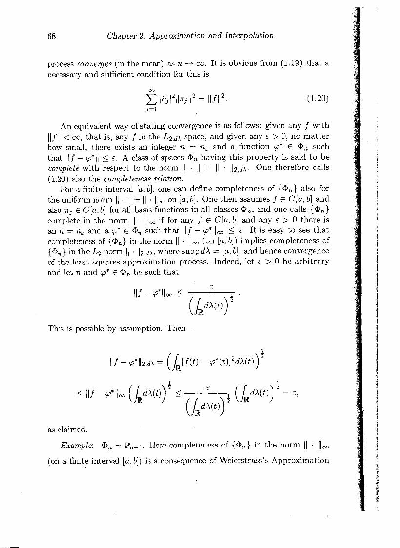
For a finite interval [a, b], one can define completeness of {a,} also for the uniform norm I( I ( = / I . )I, on [a, b]. One then assumes f E C[a, b] and also rj E C[a, b] for all basis functions in all classes a,, and one calls {a,} complete in the norm I ( . 11, if for any f E C[a, b] and any E > 0 there is an n = n, and a cp* E an such that 11 f - cp*II, 5 E. It is easy to see that completeness of {a,} in the norm ( 1 . (1, (on [a, b]) implies completeness of {@,} in the L2 norm ( 1 - ( / 2 , d A , where supp dX = [a, b], and hence convergence of the least squares approximation process. Indeed, let E > 0 be arbitrary and let n and cp* E a, be such that
C
This is possible by assumption. Then
as claimed.
Example: an = Here completeness of {a,} in the norm ( 1 (1, (on a finite interval [a, b ] ) is a consequence of Weierstrass's Approximation
51.4. Examples of orthogonal system 69
Theorem. Thus, polynomial least squares approximation on a finite interval always converges (in the mean).
51.4. Examples of orthogonal systems. There are many orthogonal systems in use. The prototype of them all is the system of trigonometric functions known from Fourier analysis. Other widely used systems involve algebraic polynomials. We restrict ourselves here to these two particular examples of orthogonal systems.
(1) Tm'gonometm'c functions: 1, cost, cos2t, cos3t , . . . , sint , sin2t, sin 3t, . . . . These are the basic harmonics; they are mutually orthogonal on the interval [O,2n] with respect to .the equally weighted measure on [ 0 , 2 ~ ] ,
dt on [0,2n], dX(t) =
0 otherwise .
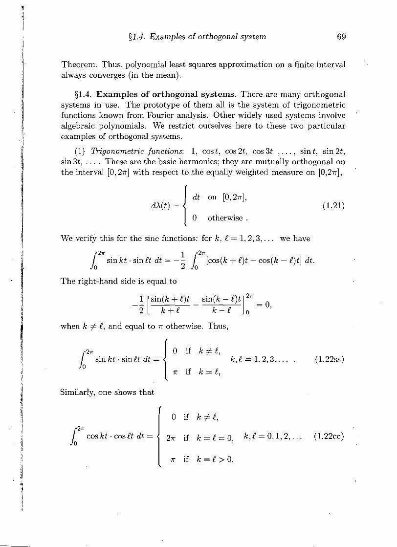
We verify this for the sine functions: for k, l = 1,2 ,3 , . . . we have
i2" sin kt . sin l t dt = - - 2
[cos(k + l ) t - cos(k - l ) t] dt.
The right-hand side is equal to
when k # l, and equal to rr otherwise. Thus,
6'" 0 if k # l,
sin kt sin l t dt = k , l = l , 2 , 3 , . . . . ( 1 . 2 2 4
rr if k = l,
Similarly, one shows that
51.4. Examples of orthogonal system
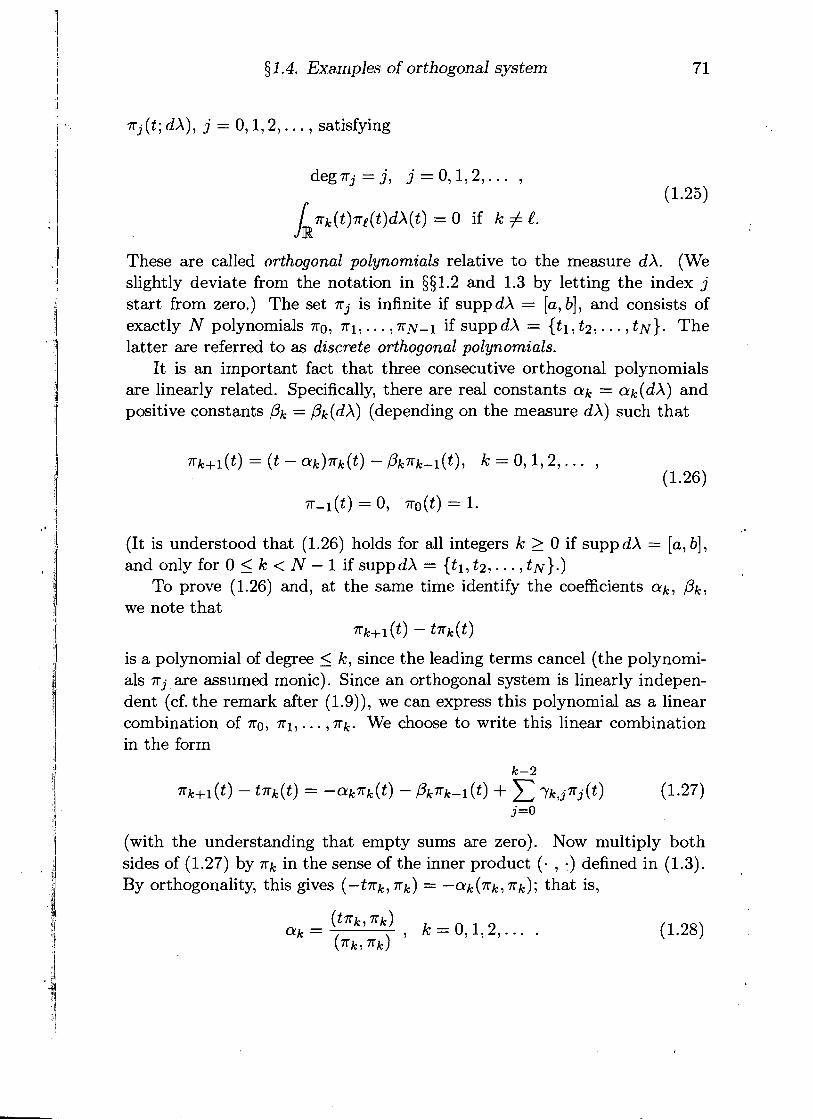
r j ( t ; dX), j = 0,1,2,. . . , satisfying
These are called orthogonal polynomials relative to the measure dX. (We slightly deviate from the notation in 551.2 and 1.3 by letting the index j start from zero.) The set rj is infinite if suppdX = [a, b], and consists of exactly N polynomials TO, rl, . . . , r ~ - l if supp dX = {t 1, t2, . . . , tN). The latter are referred to as discrete orthogonal polynomials.
It is an important fact that three consecutive orthogonal polynomials are linearly related. Specifically, there are real constants cur, = cuk(dX) and positive constants Pk = Pk(dX) (depending on the measure dX) such that
(It is understood that (1.26) holds for all integers k 2 0 if supp dX = [a, b], and only for 0 5 k < N - 1 if suppdX = {tl, t2,. . . , t ~ ) . )
To prove (1.26) and, at the same time identify the coefficients cuk, Pk, we note that
~ k + l (t) - t ~ k ( t )
is a polynomial of degree 5 k, since the leading terms cancel (the polynomi- als rj are assumed monic). Since an orthogonal system is linearly indepen- dent (cf. the remark after (1.9)), we can express this polynomial as a linear combination of r o , rl, . . . , rk. We choose to write this linear combination in the form
(with the understanding that empty sums are zero). Now multiply both sides of (1.27) by r k in the sense of the inner product (. , .) defined in (1.3). By orthogonality, this gives (-tnk, rk) = --ak ( rk , rk) ; that is,
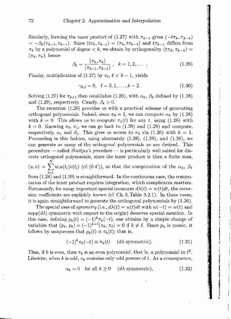
72 Chapter 2. Approximation and Interpolation
Similarly, forming the inner product of (1.27) with nk-l.gives (-tnk, 7rk-l) = rkm1). Since (t.rrk, ~ k - 1 ) = (nk, tnk-1) and differs from nk by a polynomial of degree < k, we obtain by orthogonality (t.rrk, .rrk- l ) = (nk, nk); hence
Finally, multiplication of (1.27) by 9, e < k - 1, yields
Solving (1.27) for nk+l then establishes (1.26), with a k , pk defined by (1.28) and (1.29), respectively. Clearly, Pk > 0.
The recursion (1.26) provides us with a practical scheme of generating orthogonal polynomials. Indeed, since no = 1, we can compute a 0 by (1.28) with k = 0. This allows us to compute nl( t ) for any t, using (1.26) with Ic = 0. Knowing no, nl, we can go back to (1.28) and (1.29) and compute, respectively, a1 and PI. This gives us access to .rr2 via (1.26) with k = 1. Proceeding in this fashion, using alternately (1.28), (1.29), and (1.26), we can generate as many of the orthogonal polynomials as are desired. This procedure - called Stieltjes's procedure - is particularly well suited for dis- crete orthogonal polynomials, since the inner product is then a finite sum,
N
(u, z)) = ~ ~ t l ( t ~ ) t l ( t ~ ) (cf. (0.4')), SO that the comphtation of the a k , Pk i= 1
from (1.28) and (1.29) is straightforward. In the continuous case, the compu- tation of the inner product requires integration, which complicates matters. Fortunately, for many important special measures dX(t) = w(t)dt, the recur- sion coefficients are explicitly known (cf. Ch. 3, Table 3.2.1). In these cases, it is again straightforward to generate the orthogonal polynomials by (1.26).
The special case of symmetry (i.e., dX(t) = w(t)dt with w(-t) = w(t) and supp(dX) symmetric with respect to the origin) deserves special mention. In this case, defining pk(t) = (-l)knk(-t), one obtains by a simple change of variables that (pk, pe) = (-l)k+P(rrk, re) = 0 if k # e. Since pk is monic, it follows by uniqueness that pk(t) = nk(t); that is,
(- l ) k ~ k ( - t ) 3 ?ik(t) ( d ~ symmetric). (1.31)
Thus, if k is even, then nk is an even polynomial, that is, a polynomial in t2. Likewise, when k is odd, .irk contains only odd powers 0f.t. As a consequence,
al, = O for all k 2 0 (dX symmetric), (1.32)
51.4. Examples of orthogonal system 73
which also follows from (1.28), since the numerator on the right of this equation is an integral of an odd function over a symmetric set of points.
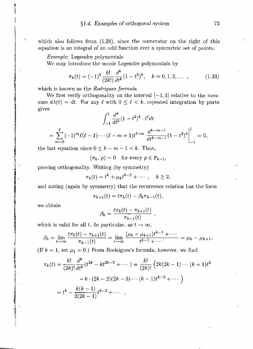
Example: Legendre polynomials We may introduce the monic Legendre polynomials by
which is known as the Rodrigues formula. We first verify orthogonality on the interval [- 1,1] relative to the mea-
sure dX(t) = dt. For any l with 0 5 C < k, repeated integration by parts gives
the last equation since 0 5 k - m - 1 < k. Thus,
(rk, p) = 0 for everyp E Pk-l,
proving orthogonality. Writing (by symmetry)
r k ( t ) = tk + pktk-2 + - . - , k > 2,
and noting (again by symmetry) that the recurrence relation has the form
we obtain
which is valid for all t. In particular, as t + oo,
t rk(t) - rk+l (t) ( ~ k - pk+lIt lC-l+. . . pk = lim = lim -
t'm ~ & ~ ( t ) t'ca tk-1 + . . . - pk - pk+l.
(If k = 1, set p1 = 0.) From Rodrigues's formula, however, we find
74 Chapter 2. Approxima tion and Interpolation
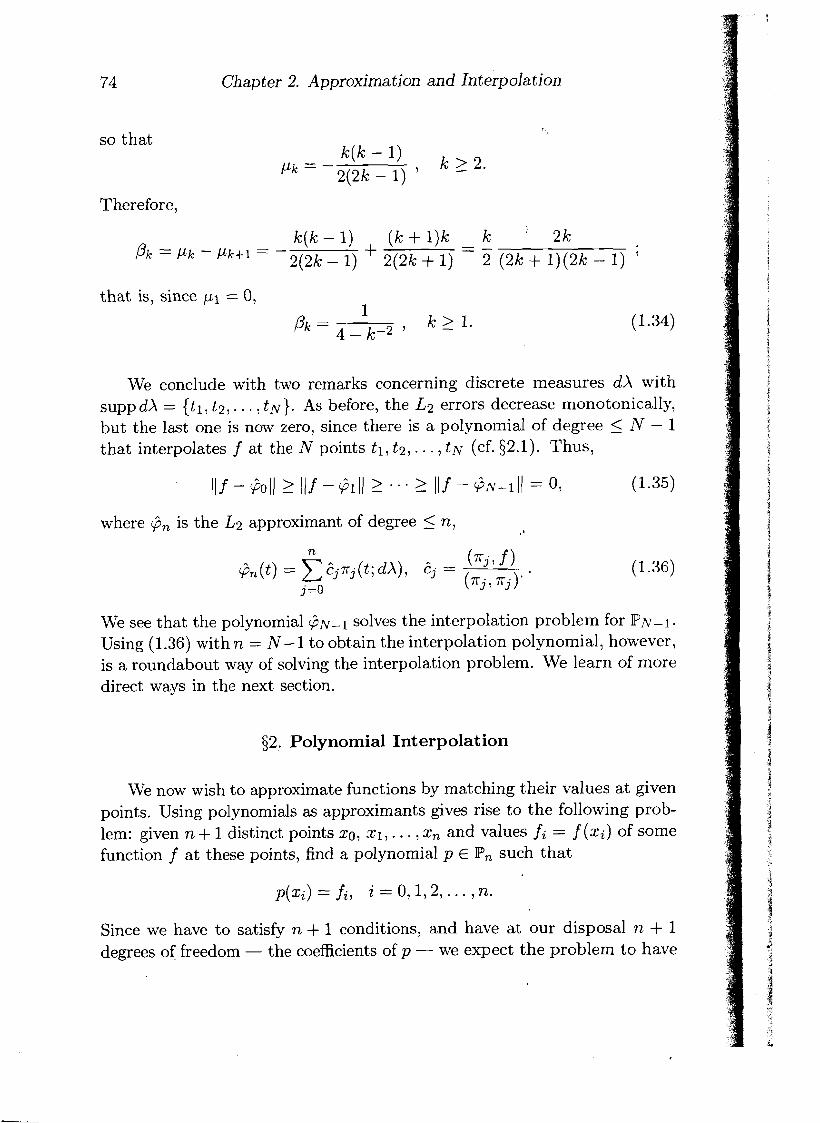
so that
Therefore,
that is, since p1 = 0, I
We conclude with two remarks concerning discrete measures dX with supp dX = i t l , t2 , . . . , tN}. As before, the L2 errors decrease monotonically, but the last one is now zero, since there is a polynomial of degree 5 N - I that interpolates f at the N points t l , t2, . . . , t~ (cf. $2.1). Thus,
where @, is the L2 approximant of degree 5 n,
We see that the polynomial GNml solves the interpolation problem for IPN-~. Using (1.36) with n = N - 1 to obtain the interpolation polynomial, however, is a roundabout way of solving the interpolation problem. We learn of more direct ways in the next section.
52. Polynomial Interpolation
We now wish to approximate functions by matching their values a t given points. Using polynomials as approximants gives rise to the following prob- lem: given n + 1 distinct points xo, XI , . . . , xn and values fi = f (xi) of some function f a t these points, find a polynomial p E P, such that
Since we have to satisfy n + 1 conditions, and have a t our disposal n + 1 degrees of: freedom - the coefficients of p - we expect the problem to have
$2. Polynomial Interpolation 75
a unique solution. Other questions of interest, in addition to existence and uniqueness, are different ways of representing and computing the polyno- mial p, what can be said about the error e(x) = f (x) - p(x) when x # xi, i = 0, 1, . . . , n, and the quality of approximation f (x) = p(x) when the number of points, and hence the degree of p, is allowed to increase indefi- nitely. Although these questions are not of the utmost interest in themselves, the results discussed here are widely used in the development of approxi- mate methods for more important practical tasks such as solving initial and boundary value problems for ordinary and partial differential equations. I t is in view of these and other applications that we study polynomial interpo- lation.
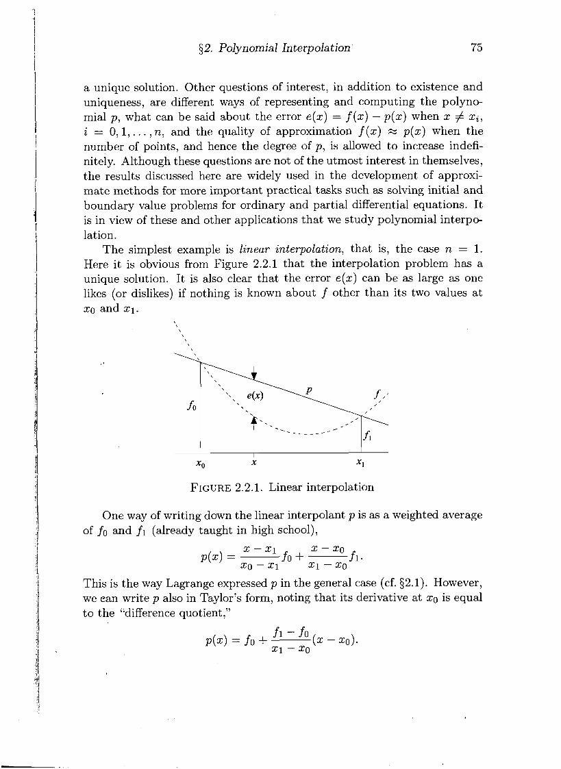
The simplest example is linear interpolation, that is, the case n = 1. Here it is obvious from Figure 2.2.1 that the interpolation problem has a unique solution. It is also clear that the error e(x) can be as large as one likes (or dislikes) if nothing is known about f other than its two values at xo and XI.
\
FIGURE 2.2.1. Linear interpolation
One way of writing down the linear interpolant p is as a weighted average of fo and f l (already taught in high school),
This is the way Lagrange expressed p in the general case (cf. $2.1). However, we ean write p also in Taylor's form, noting that its derivative at xo is equal to the "difference quotient,"
I I § 2.1. Lagrange interpolation formula; interpolation operator 77
is a polynomial of degree 5 n that satisfies
In other words, d has n + 1 distinct zeros xi. There is only one polynomial in P,' with that many zeros, namely, d(x) 0. Therefore, p*(x) = ~ ( x ) .
We denote the unique polynomial p E Pn interpolating f at the (distinct) points xo, X I , . . . , xn by
I P n ( f ; x ~ , x l r 1xn;x) = Pn(flx); (2.3)
where we use the long form on the left if we want to place in evidence the points at which interpolation takes place, and the short form on the right if the choice of these points is clear from the context. We thus have what is called the ~ a ~ r a n ~ e ' interpolation formula
withlothe f i(x) - the elementary Lagrange interpolation polynomials - de- fined in (2.1).
It is useful to look at Lagrange interpolation in terms of a (linear) oper- ator Pn from (say) the space of continuous functions to the space of poly- nomials P,,
P n : C[a,b] *Pn, P ( . ) =Pn(f : 0 ) -
I (2.5)
!
The interval [a, b] here is any interval containing all points xi, i = 0; 1: . . . , n. The operator Pn has the following properties.
I (i) P n ( ~ f ) =ctPnf, Q E R (homogeneity);
i (ii) Pn( f + g) = Pn f + P,g (additivity).
i ' ~ o s e ~ h Louis Lagrange (1736-1813), born in Turin, became, through correspondence
i with Euler, his protkgk. In 1766 he indeed succeeded Euler in Berlin. He returned to Paris in 1787. Clairaut wrote of the young Lagrange: '' . . . a young man, no less remarkable for his talents than for his modesty; his temperament is mild and melancholic: he knows no other pleasure than study." Lagrange made fundamental contributions to the calculus of variations and to number theory, but worked also on many problems in analysis. He is widely known for his representation of the remainder term in Taylor's formula. The
I interpolation formula appeared in 1794. His Me'canique Analytique, published in 1788,
1 !
made him,one of the founders of analytic mechanics.
78 Chapter 2. Approxima tion and Interpolation
Combining (i) and (ii) shows that Pn is a linear operator,
Pn(af +Pg) = aPnf fPPn9 , a , P E R -
(iii) P, f = f for all f E P,.
The last property - an immediate consequence of uniqueness of the in- terpolation polynomial - says that Pn leaves polynomials of degree < n unchanged, and hence is a projection operator.
A norm of the linear operator Pn can be defined (similarly as for matrices, cf. Ch. 1, (3.11)) by
where on the right one takes any convenient norm for functions. Taking the L, norm (cf. Table 2.0.1), one obtains from Lagrange's formula (2.4)
Indeed, equality holds for some continuous function f ; cf. Ex. 27. Therefore,
where
The function Xn(x) and its maximum An are called, respectively, the Lebesgue2 function and Lebesgue constant for Lagrange interpolation. They provide a first estimate for the interpolation error: let En(f) be the best (uniform) approximation of f by polynomials of degree 5 n,
2Henri Lebesgue (1875-1941) was a French mathematician known for his fundamental work on the theory of real functions, notably the concepts of measure and integral that no* bear his name.
$ 2.2. Interpolation error
where 6, is the nth-degree polynomial of best uniform approximation to f . Then, using the basic properties (i) through (iii) of Pn, in particular, the projection property (iii), and (2.7) and (2.9), one finds
that is, / I f - pn ( f ; . )IIm I (1 + An)&n(f)- (2.11)
Thus, the better f can be approximated by polynomials of degree 5 n , the smaller the interpolation error. Unfortunately, An is not uniformly bounded: no matter how one chooses the nodes xi = xin), i = O , l , . . . , n , one can show that always An > O(1og n) as n -+ oo. It is not possible, therefore, to conclude from Weierstrass's approximation theorem (i.e., from En (f ) -+ 0, n -+ oo) that Lagrange interpolation converges uniformly on [a, b] for any continuous function, not even for judiciously selected nodes; indeed, one knows that it does not.
$2.2. Interpolation error. As noted earlier, we need to make some assump,tions about the function f in order to be able to estimate the error of interpolation, f (x) - pn( f ; x), for any x # Xi in [a, b]. In (2.11) we made an assumption in terms of how well f can be approximated on [a, b] by polynomials of degree 5 n. Now we make an assumption on the magnitude of some appropriate derivative of f .
It is not difficult to guess how the formula for the error should look: since the error is zero at each xi, i = 0,1 , . . . , n , we ought to see a factor of the form (x - xo) (x - x l ) . . . (x - 2,). On the other hand, by the projection property (iii) in $2.1, the error is also zero (even identically so) if f E Pn, which suggests another factor - the (n+ 1)st derivative of f . But evaluated where? Certainly not at x , since f would then have to satisfy a differential equation. So let us say that f ("+'I is evaluated at some point ( = ((x) , which is unknown but must be expected to depend on x. Now if we test the formula so far conjectured on the simplest nontrivial polynomial, f (z) = xn+l , we discover -that a factor l / (n + I)! is missing. So, our final (educated) guess is the formula
80 Chapter 2. Approximation and Interpolation
Here <(x) is some number in the open interval (a, b), but otherwise unspec- ified,
a < <(x) < b. (2.13)
The statement (2.12) and (2.13) is, in fact, correct if we assume that f E c"+' [a, b]. An elegant proof of it, due to C a ~ c h ~ , ~ goes as follows. We can assume x # xi for i = 0,1, . . . , n, since otherwise (2.12) would be trivially true for any <(x). So, fix x E [a, b] in this manner, and define a function F of the new variable t as follows,
Clearly, F E C n f l [a, b] . Furthermore,
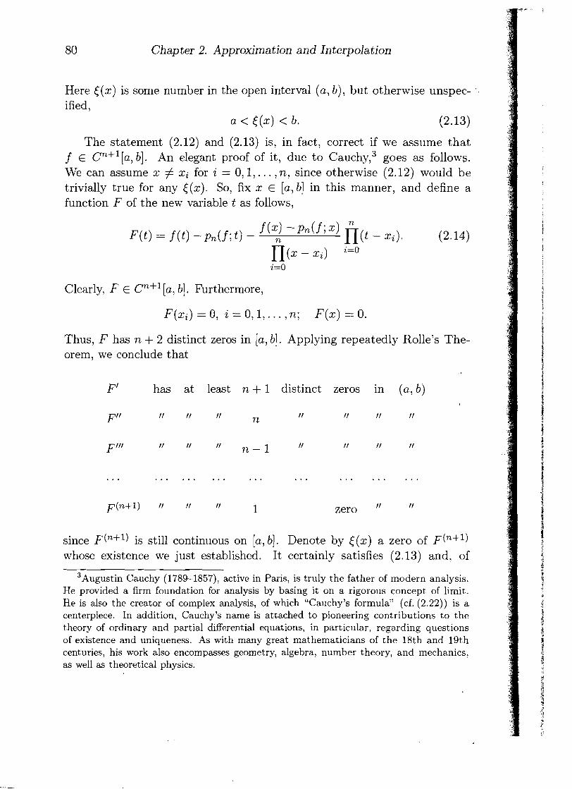
Thus, F has n + 2 distinct zeros in [a, b]. Applying repeatedly Rolle's The- orem, we conclude that
F' has at least n + 1 distinct zeros in ( a , b)
~ ( n + 1 ) f l I I II 1 zero II I I
since F("+') is still continuous on [a, b]. Denote by <(x) a zero of F ( n+l) whose existence we just established. It certainly satisfies (2.13) and, of
3~ugus t in Cauchy (1789-1857), active in Paris, is truly the father of modern analysis. He provided a firm foundation for analysis by basing it on a rigorous concept of limit. He is also the creator of complex analysis, of which "Cauchy's formula" (cf. (2.22)) is a centerpiece. In addition, Cauchy's name is attached to pioneering contributions to the theory of ordinary and partial differential equations, in particular, regarding questions of existence and uniqueness. As with many great mathematicians of the 18th and 19th centuries, his work also encompasses geometry, algebra, number theory, and mechanics, as well as theoretical physics.
fj 2.2. Interpolation error
course, will depend on 'x. Now differentiating F in (2.14) n + 1 times with respect to t , and then setting t = <(x), we get
which, when solved for f (x) -p,( f ; x), gives precisely (2.12). Actually, what we have shown is that J(x) is contained in the span of xo, X I , . . . , x,, x, that is, in the interior of the smallest closed interval containing xo, X I , . . . , x, and x.
Examples.
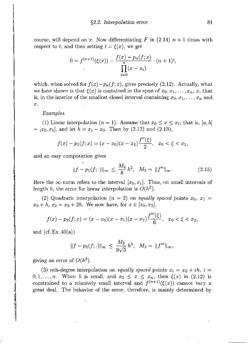
(1) Linear interpolation (n = 1). Assume that xo < x < XI; that is, [a, b] = [xo, xl], and let h = XI - xo. Then by (2.12) and (2.13),
and an easy computation gives
Here the oo-norm refers to the interval [xO, xl]. Thus, on small intervals of length h, the error for linear interpolation is 0 ( h 2 ) .
(2) Quadratic interpolation (n = 2) on equally spaced points xo, x l = xo + h, x:! = xo + 2h: We now have, for x E [xo, x2],
and (cf. Ex. 40(a))
M3 h3, M3 = 1 1 f ' " l l m , llf - p2(f; .)IIm < q
giving an error of O(h3).
(3) nth-degree interpolation on equally spaced points xi = xo + ih, i =
0 1 . . . , n. When h is small, and xo 5 x 5 x,, then <(x) in (2.12) is constrained to a relatively small interval and f (n+l)(<(x)) cannot vary a great deal. The behavior of the error, therefore, is mainly determined by
Chapter 2. Approximation and Interpolation
n
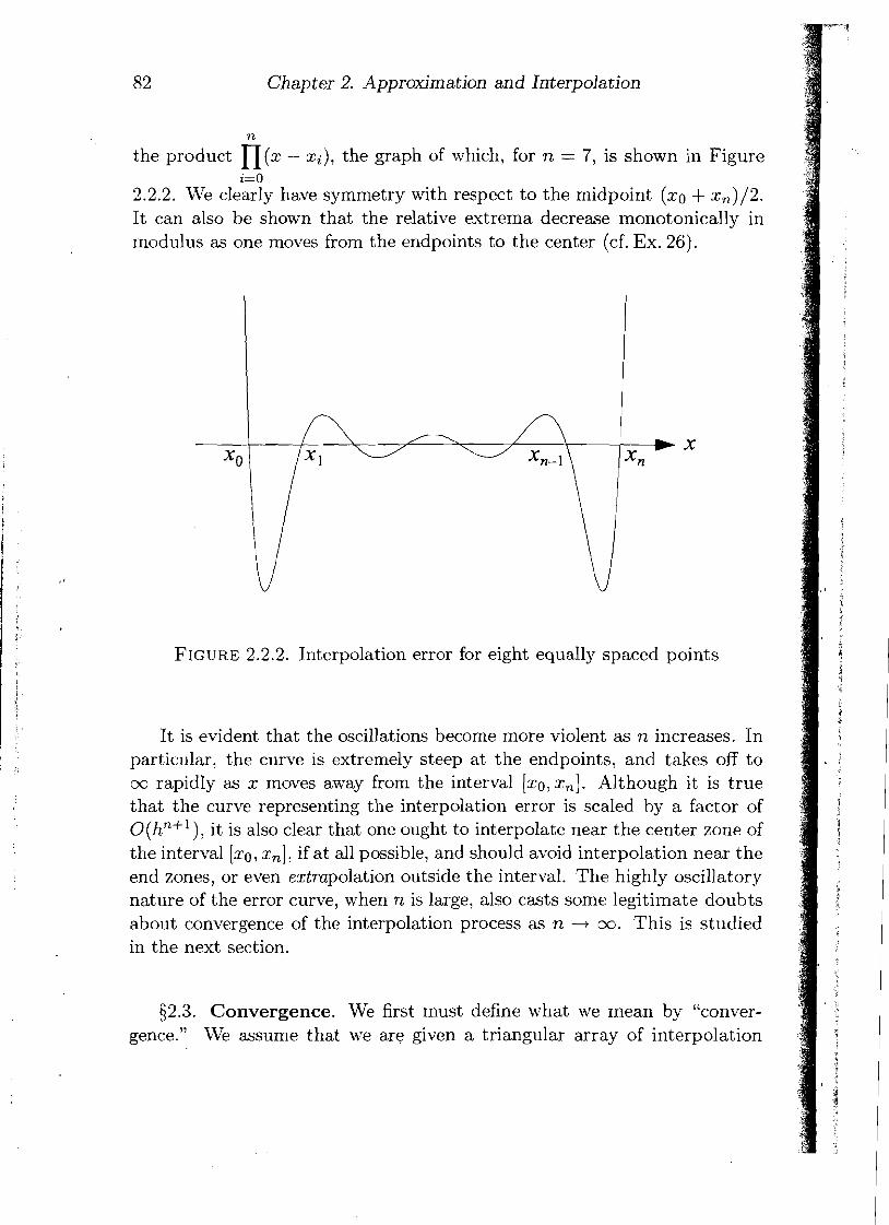
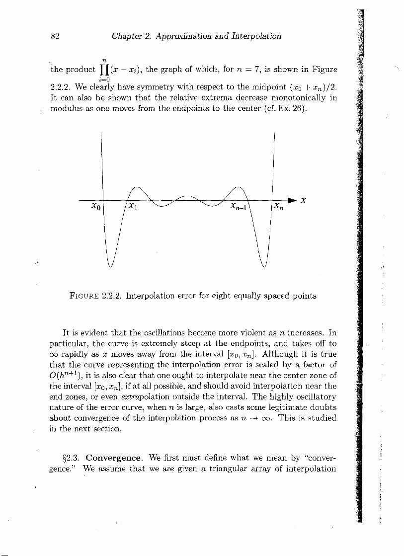
the product n ( x - xi), the graph of which, for n = 7, is shown in Figure i=O
2.2.2. We clearly have symmetry with respect to the midpoint (xo + xn)/2. It can also be shown that the relative extrema decrease monotonically in modulus as one moves from the endpoints to the center (cf. Ex. 26).
FIGURE 2.2.2. Interpolation error for eight equally spaced points
It is evident that the oscillations become more violent as n increases. In particular, the curve is extremely steep at the endpoints, and takes off to GO rapidly as x moves away from the interval [xo,xn]. Although it is true that the curve representing the interpolation error is scaled by a factor of O(hn+'), it is also clear that one ought to interpolate near the center zone of the interval [xo, x,], if at all possible, and should avoid interpolation near the end zones, or even extrapolation outside the interval. The highly oscillatory nature of the error curve, when n is large, also casts some legitimate doubts about convergence of the interpolation process as n -+ oo. This is studied in the next section.
52.3. Convergence. We first must define what we mean by "conver- gence." We assume that we are given a triangular array of interpolation
fj 2.3. Convergence
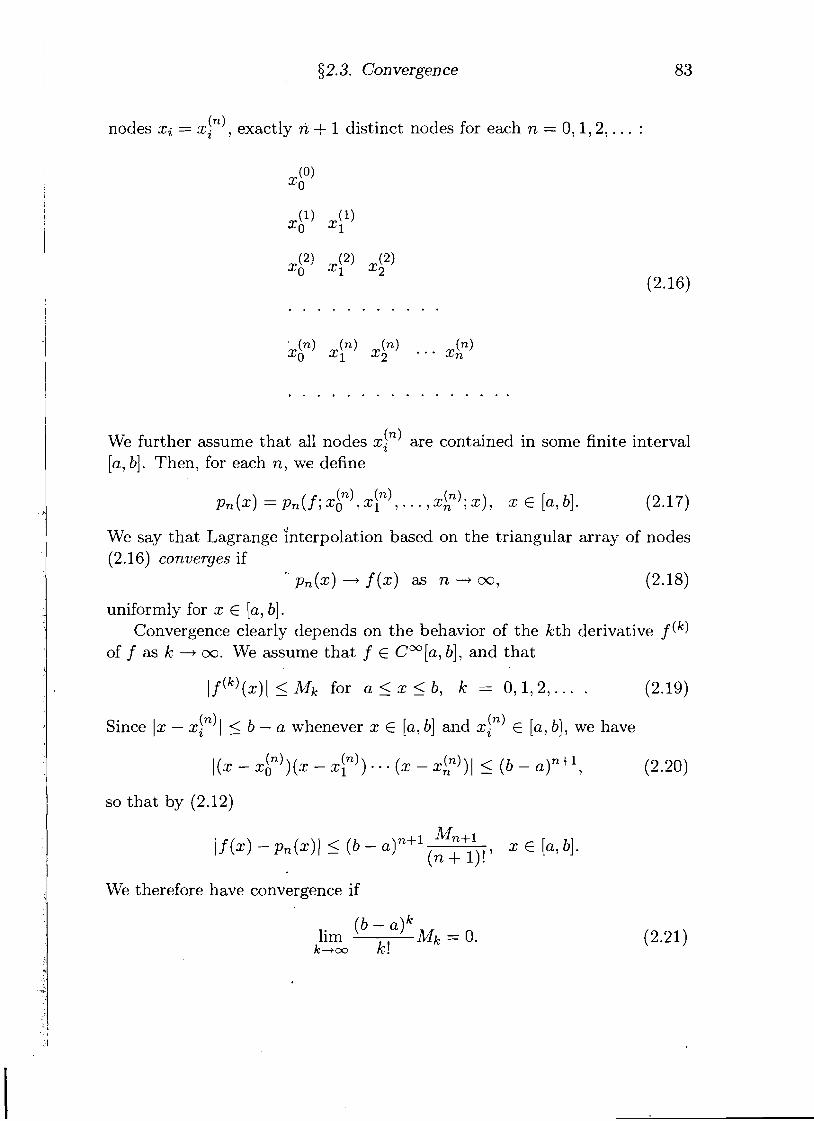
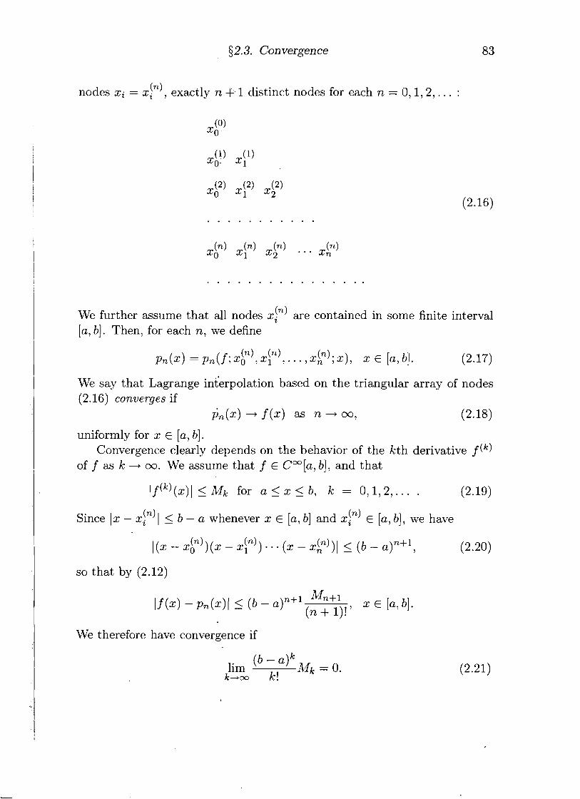
. . nodes xi = xin), exactly n+ 1 distinct nodes for each n = 0 , 1 , 2 , . :
We further assume that all nodes xin) are contained in some finite interval [a, b]. Then, for each n, we define
We say that Lagrange 'i'nterpolation based on the triangular array of nodes (2.16) converges if
pn(x ) -+ f ( x ) as n - - t m l (2.18)
uniformly for x E [a, b]. Convergence clearly depends on the behavior of the kth derivative f ( k )
of f as k -+ oo. We assume that f E C m [ a , b] , and that
. . . . . ~ f ( ~ ) ( x ) l 5 Mk for a 5 x 5 b, k = 0 , 1 , 2 (2.19)
Since lz - xin)l 5 b - a whenever x E [a , b] and xin) E [a , b] , we have
so that by (2.12)
- a)"+' Mn+l I f ( x ) - pn(x)l 5 ( b (n + I ) ! ' x E [a, b].
We therefore have convergence if
( b - a ) k lim M k = 0.
k + m k!
Chapter 2. Approximation and Interpolation
n
the product n ( x - xi), the graph of which, for n = 7, is shown in Figure i=O
2.2.2. We clearly have symmetry with respect to the midpoint (xo + xn)/2. It can also be shown that the relative extrema decrease monotonically in modulus as one moves from the endpoints to the center (cf. Ex. 26).
FIGURE 2.2.2. Interpolation error for eight equally spaced points
It is evident that the oscillations become more violent as n increases. In particular, the curve is extremely steep at the endpoints, and takes off to cu rapidly as x moves away from the interval [xo,x,]. Although it is true that the curve representing the interpolation error is scaled by a factor of O(hn+l), it is also clear that one ought to interpolate near the center zone of the interval [xo, x,], if at all possible, and should avoid interpolation near the end zones, or even extrapolation outside the interval. The highly oscillatory nature of the error curve, when n is large, also casts some legitimate doubts about convergence of the interpolation process as n -+ oo. This is studied in the next section.
52.3. Convergence. We first must define what we mean by "conver- gence." We assume that we are given a triangular array of interpolation
5 2.3. Convergence
. . nodes xi = X I " ) , exactly n + 1 distinct nodes for each n = 0 , 1 , 2 , . :
We further assume that all nodes xin) are contained in some finite interval [a, b]. Then, for each n, we define
("1 ("1 pn(x) = p n ( f ; so , xl , - . , X ) x ) , x E [a, b]. (2.17)
We say that Lagrange inkrpolation based on the triangular array of nodes (2.16) converges if
Ijn(x) + f ( x ) as n+m, (2.18)
uniformly for x E [a, b] . Convergence clearly depends on the behavior of the kth derivative f (k)
of f as k + oo. We assume that f E Cm [a, b] , and that
~ f ( ~ ) ( x ) l < Mk for a < x < b, k = 0 , 1 , 2 , . . . . (2.19)
Since 12: - xjn)l < b - a whenever x E [a, b] and xin) E [a, b], we have
so that by (2.12)
Mn+l I f ( X I - ~ n ( x ) I < (b - a)"+' (n + 7 x E [a, b].
We therefore have convergence if
(b - a ) k lim Mk = 0.
k+m k!
Chapter 2. Approxima tion and Interpolation
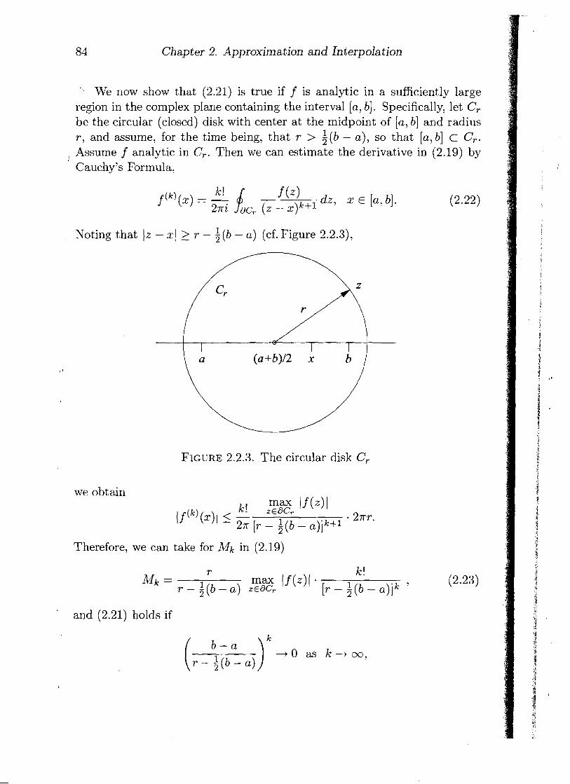
' . We now show that (2.21) is true if f is analytic in a sufficiently large region in the complex plane containing the interval [a, b] . Specifically, let C, be the circular (closed) disk with center at the midpoint of [a, b] and radius r, and assume, for the time being, that r > 4 (b - a), s o that [a, b] c C,.
, Assume f analytic in C,. Then we can estimate the derivative in (2.19) by Cauchy's Formula,
k ! f (z) dz, x ~ [ a , b ] .
( z - x ) ~ + ~
Noting that lz - sl 2 T - i ( b - a) (cf. Figure 2.2.3),
FIGURE 2.2.3. The circular disk C,
Therefore, we can take for Mk in (2.19)
and (2.21) holds if
k b-a
-+ 0 as k -+ cm,
5 2.3. Convergence
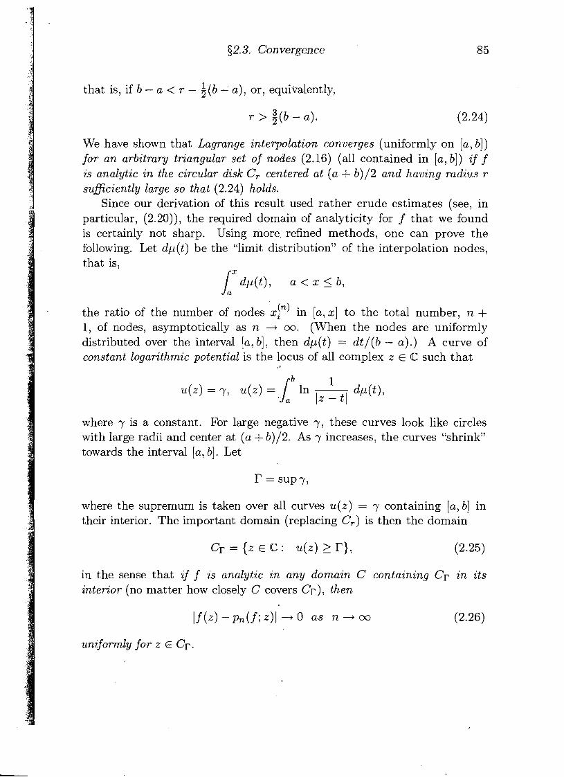
that is, if b - a < r - i ( b - a) , o r , equivalently,
r > g ( b - a) .
We have shown that Lagrange interpolation converges (uniformly on [a, b]) for an arbitrary triangular set of nodes (2.16) (all contained in [a, b]) if f is analytic in the circular disk C, centered at (a + b)/2 and having radius r suficiently large so that (2.24) holds.
Since our derivation of this result used rather crude estimates (see, in particular, (2.20)), the required domain of analyticity for f that we found is certainly not sharp. Using more, refined methods, one can prove the following. Let dp(t) be the "limit distribution" of the interpolation nodes, that is,
the ratio of the number of nodes xin) in [a, x] to the total number, n + 1, of nodes, asymptotically as n -+ oo. (When the nodes are uniformly distributed over the interval [a, b], then dp(t) = dt/(b - a).) A curve of constant logarithmic potential is the locus of all complex z E @ such that
where y is a constant. For large negative y , these curves look like circles with large radii and center at (a + b)/2. As y increases, the curves "shrink" towards the interval [a, b]. Let
where the supremum is taken over all curves u(z) = y containing [a, b] in their interior. The important domain (replacing C,) is then the domain
in the sense that if f is analytic in any domain C containing Cr in its interior (no matter how closely C covers Cr), then
uniformly for z E Cr.
Examples. .
Chapter 2. Approximation and Interpolation
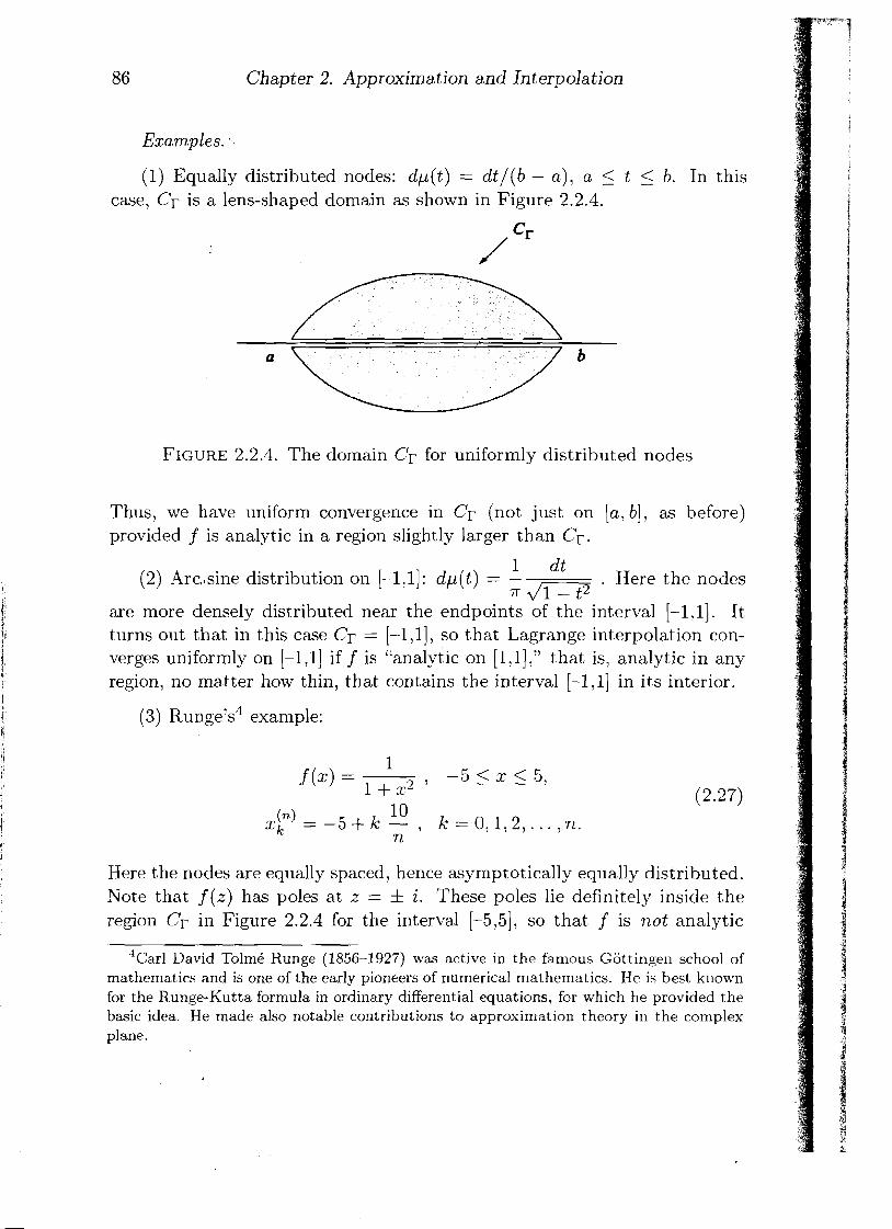
(1) Equally distributed nodes: dp(t) = dt/(b - a) , a 5 t 5 b. In this case, Cr is a lens-shaped domain as shown in Figure 2.2.4.
CF
FIGURE 2.2.4. The domain Cr for uniformly distributed nodes
Thus, we have uniform convergence in Cr (not just on [a , b], as before) provided f is analytic in a region slightly larger than Cr.
1 dt (2) Arconsine distribution on [-1!1]: dp(t) = - . Here the nodes
n JF7 are more densely distributed near the endpoints of the interval [-1,1]. It turns out that in this case Cr = [-1,1], so that Lagrange interpolation con- verges uniformly on [-1,1] if f is "analytic on [1,1]," that is, analytic in any region, no matter how thin, that contains the interval [-1,1] in its interior.
(3) ~ u n ~ e ' s ~ example:
Here the nodes are equally spaced, hence asymptotically equally distributed. Note that f ( z ) has poles at z = f i. These poles lie definitely inside the region Cr in Figure 2.2.4 for the interval [-5,5], so that f is not analytic
4 ~ a r l David Tolmk Runge (1856-1927) was active in the famous Gottingeil school of mathematics and is one of the early pioneers of numerical mathematics. He is best known for the Runge-Kutta formula in ordinary differential equations, for which he provided the basic idea. He made also notable contributions to approximation theory in the complex plane.
52.3. Convergence 87
in Cr . For this reason, we can no longer expect convergence on the whole interval [-5,5]. It has been shown, indeed, that
We have convergence in the central zone of the interval [-5,5], but divergence in the lateral zones. With Figure 2.2.2 kept in mind, this is perhaps not all that surprising (cf. Mach. Ass. 7(b)).
(4) Bernstein's5 example:
Here analyticity of f is completely gone, f being not even differentiable at x = 0. Accordingly one finds that
lim I f ( x ) - p n ( f ; x ) J = m fo r every x E [-1,1], n-+m
except x = -1, x = 0, and x = 1.
The fact that x = f 1 are exceptional points is trivial, since they are inter- polation nodes, where the error is zero. The same is true for x = 0 when n is even, but not if n is odd.
The failure of convergence in the last two examples can only in part be blamed on insufficient regularity of f . Another culprit is the equidistribution of the nodes. There are indeed better distributions, for example, the arc sine distribution of Example (2 ) . An instance of the latter is discussed in the next section.
We add one more example, which involves complex nodes, and for which the preceding theory, therefore, no longer applies. We prove convergence directly.
5Sergei Natanovii: BernStein (1880-1968) made major contributions to polynomial ap- proximation, continuing in the tradition of his countryman Chebyshev. He is also known for his work on partial differential equations and probability theory.
88 Chapter 2. Approximation and Interpolation
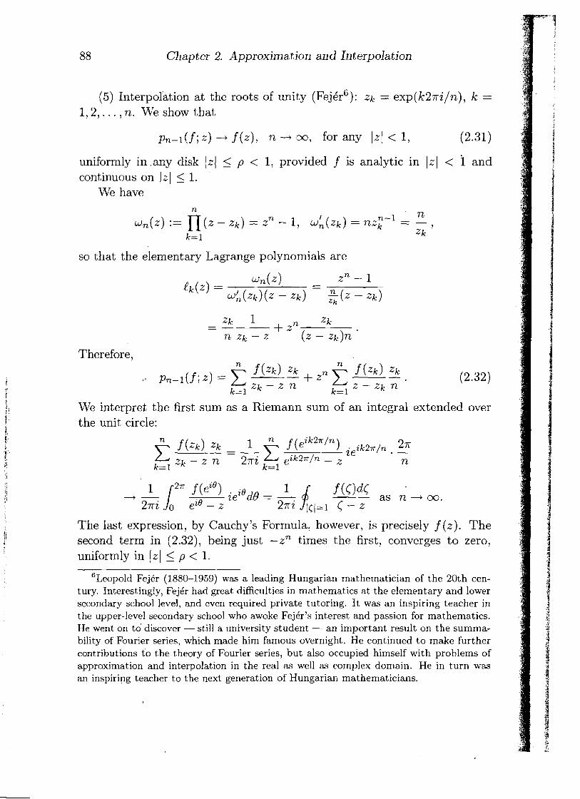
(5) ~nter~ola t ion at the roots of unity (FejBr6): zk = exp(k27ri/n), k = 1,2, . . . , n. We show that
uniformly in .any disk lzJ < p < 1, provided f is analytic in J z J < 1 and continuous on J z J 5 1.
We have
so that the elementary Lagrange polynomials are
- - Zk 1 -- + zn zk
n z k - z (2 - zk)n '
Therefore,
We interpret the first sum as a Riemann sum of an integral extended over the unit circle:
The last expression, by Cauchy's Formula, however, is precisely f (2). The second term in (2.32), being just -zn times the first, converges to zero, uniformly in lz 5 p < 1.
' ~ e o ~ o l d Fej6r (1880-1959) was a leading Hungarian mathematician of the 20th cen- tury. Interestingly, Fejkr had great difficulties in mathematics at the elementary and lower secondary school level, and even required private tutoring. It was an inspiring teacher in the upper-level secondary school who awoke Fejkr's interest and passion for mathematics. He went on t o discover - still a university student - an important result on the summa- bility of Fourier series, which made him famous overnight. He continued to make further contributions to the theory of Fourier series, but also occupied himself with problems of approximation and interpolation in the real as well as complex domain. He in turn was an inspiring teacher to the next generation of Hungarian mathematicians.
52.4. Chebyshev polynomials and nodes 89
52.4. Chebyshev polynomials and nodes. The choice of nodes, as we saw in the previous section, distinctly influences the convergence char- acter of the interpolation process. We now discuss a choice of points - the Chebyshev points - which leads to very favorable convergence properties. These points are useful, not only for interpolation, but also for other pur- poses (integration, collocation, etc.) . We consider them on the canonical interval [-1,1], but they can be defined on any finite interval [a, b] by means of a linear transformation of variables that maps [-1,1] onto [a, b].
We begin with developing the Chebyshev polynomials. They arise from the fact that the cosine of a multiple argument is a polynomial in the cosine of the simple argument; more precisely, *
This is a consequence of the well-known trigonometric identity
cos(k + 1)0 + cos(k - 1)0 = 2 cos 0 cos k0,
which, when solved for the first term, gives
Therefore, if cos m0 is a polynomial of degree rn in cos 0 for all m 5 k, then the same is true for m = k + 1. at he ma tical induction then proves (2.33). At the same time, it follows from (2.34) that
The polynomials T, so defined are called the Chebyshev polynomials (of the first kind). Thus, for example,
and so on.
90 Chapter 2. Interpolation and Approximation
Clearly, these polynomials are defined not only for x in [-1,1], but for arbitrary real or complex x. It is only that on the interval [-1,1] they satisfy the identity (2.33) (where 8 is real).
It is evident from (2.35) that the leading coefficient of T, is 2n-1 (if n > 1); the mon.ic Chebyshev polynomial of degree n , therefore, is
The basic identity (2.33) allows us to immediately obtain the zeros xr: =
x p ) of T,: indeed, cos n0 = 0 if n0 = (2k - 1)7r/2: so that
("1 = 2k - 1 x$) = cos Ok , T , k = 1 7 2 , . . . , n .
2n
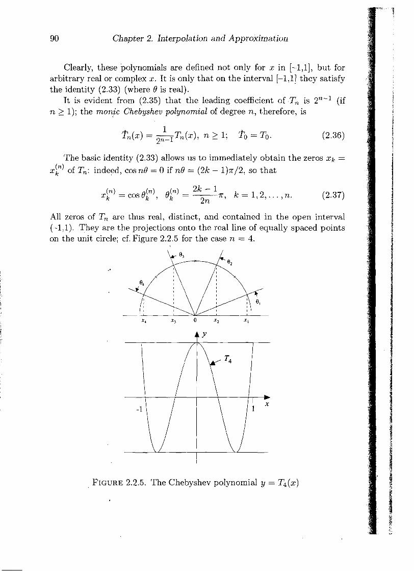
All zeros of Tn are thus real, distinct, and contained in the open interval (-1,l). They are the projections onto the real line of equally spaced points on the unit circle; cf. Figure 2.2.5 for the case n = 4.
I
FIGURE 2.2.5. The Chebyshev polynomial y = T4(x)
$2.4. Chebyshev polynomials and nodes
In terms of the zeros x p ) of Tn, we can write the mbnic polynomial in factored form as
As we let 8 increase from 0 to r, hence x = cos 8 deerease from +1 to -1, Eq. (2.33) shows that Tn(x) oscillates between +1 and -1, attaining these extreme values at
In summary, then,
2k - 1 ~ , ( x p ) ) = o for x p ) = cos r, k = 1 , 2 , . . . , n ;
2n
k ~ ~ ( y p ) ) = for = C O S - T , k = 0 , 1 , 2 , . . . , n .
n (2.41)
Chebyshev polynomials owe their importance and usefulness to the fol- lowing theorem, due to ~ h e b ~ s h e v . ~
Theorem 2.2.1. For an arbztrary monic polynomzal in of degree n , there holds
where Tn zs the monic Chebyshev polynomzal (2.36) of degree n.
Proof (by contradiction). Assume, contrary to (2.42), that
Then the polynomial dn(x) = Tn(x) -in (x) (a polynomial of degree 5 n - 1), satisfies
7Pafnuti Levovich Chebyshev (1821-1894) was the most prominent member of the St. Petersburg school of mathematics. He made pioneering contributions to number theory, probability theory, and approximation theory. He is regarded as the founder of construc- tive function theory, but also worked in mechanics, notably the theory of mechanisms, and in ballistics.
92 Chapter 2. lnterpola tion and Approxima tion
Thus dn changes sign a t least n'times, and hence has a t least n distinct real zeros. But having degree 5 n - 1, it must vanish identically, dn(x) - 0. This contradicts (2.44); thus (2.43) cannot be true.
The result (2.42) can be given the following interesting interpretation: the best uniform approximation (on the interval [-1,1]) to f (x) = xn from polynomials in Pndl is given by xn - Tn(x), that is, by the aggregate of terms of degree < n - 1 in pn taken with the minus sign. From the theory of uniform polynomial approximation it is known that the best approximant is unique. Therefore, equality in (2.42) can only hold if 6, = 'fnf,.
What is the significance of Chebyshev polynomials for interpolation? Recall (cf. (2.12)) that the interpolation error (on [-1,1], for a function f E Cn+' [- l , l ] ) is given by
The first factor is essentially independent of the choice of the nodes xi. I t is true that {(x) does depend on the xi, but we usually estimate f ("+'I by 1 1 f ("+I) (I,, which removes this dependence. On the other hand, the product in the second factor, includiAg its norm
depends strongly on the xi. It makes sense, therefore, to try to minimize (2.46) over all xi E [-I, I]. Since the product in (2.46) is a monic polynomial of degree n + l , it follows from Theorem 2.2.1 that the optimal nodes xi = ?in) in (2.45) are precisely the zeros of Tn+'; that is,
For these nodes, we then have (cf. (2.42))
Ilf ("+') Im 1 llf (9 - pR.(f; .)I100 L . - ( n + l ) ! 2 n '
One ought to compare the last factor in (2.48) with the much cruder bound given in (2.20), which, in the case of the interval [-1,1], is 2n+1.
Since by (2.45) the error curve y = f - pn(f ; .) for Chebyshev points (2.47) is essentially equilibrated (modulo the variation in the factor f ("+I)),
52.4. Che byshev polynomials and nodes
and thus free of the violent oscillations we saw for equally spaced points, we would expect more favorable convergence properties for the triangular array (2.16) consisting of Chebyshev nodes. Indeed, one can prove, for example, that
(n) (n) pn(f;Po ,el , . . . , P ~ ) ; x ) + f (x) as n i m , (2.49)
uniformly on [-1,1], provided only that f E C1 [- 1, I]. Thus we do not need analyticity of f for (2.49) to hold.
We finally remark - as already suggested by the recurrence relation (2.35) - that Chebyshev polynomials are a special case of orthogonal poly- nomials. Indeed, the measure in question is precisely (up to an unimportant constant factor) the arc sine measure
already mentioned in Example (2) of 52.3. This is easily verified from (2.33) and the orthogonality of the cosines (cf. $1.4, Eq. ( 1 . 2 2 ~ ~ ) ) :
The Fourier expansion in Chebyshev polynomials (essentially the Fourier- cosine expansion) is therefore given by
where
Truncating (2.52) with the term of degree n gives a useful polynomial approximation of degree n,
94
having an error
Chapter 2. Interpolation and Approximation
The approximation on the far right is better the faster the Fourier coefficients cj tend to zero. The error (2.54), therefore, essentially oscillates between +cn+l and -%+I as x varies on the interval [-1,1], and thus is of "uniform" size. This is in stark contrast to Taylor's expansion a t x = 0, where the nth-degree partial sum has an error proportional to xn+' on [-1 ,I].
52.5. Barycentric formula. Lagrange's formula (2.4) is attractive more for theoretical purposes than for practical computational work. I t can be rewritten, however, in a form that makes it efficient computationally, and that also allows additional interpolation nodes to be added with ease. Having the latter feature in mind, we now assume a sequential set xo, X I ,
x2,. . . of interpolation nodes and denote by p n ( f ; - ) the polynomial of degree 5 n interpolating to f a t the first n + 1 of them. We do not assume that the xi are in any particular ,order, as long as they are mutually distinct.
We introduce a triangular array of auxiliary quantities defined by
The elementary Lagrange interpolation polynomials of degree n , (2.1), can then be written in the form
n
Dividing Lagrange's formula through by 1 -- C ti (x), one finds i=O
$2.5. Barycen tric formula
that is,
This expresses the interpolation polynomial as a weighted average of the function values fi = f (xi) and is, therefore, called the barycentric formula - a slight misnomer, since the weights are not necessarily all positive. The auxiliary quantities XI") involved in (2.57) are those in the row numbered n of the triangular array (2.55). Once they have been calculated, the evaluation of pn ( f ; x) by (2.57), for any fixed x, is straightforward and cheap.
Comparison with (2.4) shows that
In order to arrive at an efficient algorithm for computing the required quantities A:"), we first note that, for k 2 1,
Furthermore, Lagrange's formula for pk( f ; . ), with f ( - ) = 1, gives
Comparing the coefficients of xk on either side (assuming k _> 1) yields
This gives us the means to compute the last quantity xF) missing in (2.58). Altogether, we arrive at the following algorithm.
Chapter 2. Interpolation and Approximation
for k = 1 ,2 , . . . , n do
This requires exactly n2 additions (including the subtractions in xi -xk) and
i n ( n + 1) divisions for computirig the n + 1 quantities X f ) , A?), . . . , A!,?) in (2.57). If we decide to incorporate the next data point (x,+l, fn+l ) , all we need to do is extend the k-loop in (2.59) through n + 1, that is, generate
the next row of auxiliary quantities Xf+'), ~(1"") 7 . . . , Xn+l ("+l). We are then ready to compute p,+l ( f ; x) from (2.57) with n replaced by n + 1.
Although (2.1') in combination with (2.59) is more efficient than (2.1) (which requires 0 ( n 3 ) operations to evaluate), it is also more exposed to the detrimental effects of rounding errors. The weak spot, indeed, is the sum- mation in the last step of (2.59),,,which is subject to significant cancellation
(k) (k) errors whenever max [Xi I is much larger than ( A k 1 . Unfortunately, this O s i l k - 1
is more often the case than not: The extent of cancellation, however, may depend on the order in which the nodes xi are arranged. I t is recommended, for given n, that they be arranged in the order of decreasing distance from their midpoint. In contrast, the formula (2.1) is devoid of numerical diffi- culties since only benign operations - multiplication and division - are involved (disregarding the formation of differences such as x - xi, which occur in both formulae).
52.6. ~ e w t o n ' s ~ formula. This is another way of organizing the work in 52.5. Although the computational effort remains essentially the same, it becomes easier to treat "confluent" interpolation points, that is, multiple points in which not only the function values, but also consecutive derivative values, are given (cf. 52.7).
*sir Isaac Newton (1643-1727) was an eminent figure of 17th century mathematics and physics. Not only did he lay the foundations of modern physics, but he was also one of the coinventors of differential calculus. Another was Leibniz, with whom he became entangled in a bitter and life-long priority dispute. His most influential work was the Principia, which not only contains his ideas on interpolation, but also his suggestion to use the interpolating polynomial for purposes of integration (cf. Ch. 3, $2.2).
I 52.6. Newton's formula
Using the same setup as in 52.5, we denote
P ~ ( x ) = p n ( f ; x ~ , x l , . . - , x n ; x ) , n z 0 , 1 , 2 , . . - . (2.60) j
I We clearly have i
I PO(X) = ao,
4
for some constants ao, a l , a2,. . . . This gives rise to a new form of the interpolat ion polynomial,
1 which iscalled Newton's fom. The constants involved can be determined,
1 in principle, by the interpolation conditions 1
fl = a0 + al(x1 - xo), 1 4
i f 2 = a0 + 4 x 2 - 20) + a2(x2 - xo)(x2 - X I ) ,
and so on, which represent a triangular, nonsingular (why?) system of linear algebraic equations. This uniquely determines the constants; for example,
a2 = f 2 - a0 - 4 x 2 - xo)
(x2 - xo)(x2 - 21)
and so on. Evidently, a, is a linear combination of fo, f l , . . . , fn , with coefficients that depend on xo, xl , . . . , x,. We use the notation
Chapter 2. Interpolation and Approxima ti011
for this linear combination, and call the right-hand side the n th divided d2fference of f relative to the nodes xo, x l , . . . , x,. Considered as a function of these n + 1 variables, the divided difference is a symmetric function; that is, permuting the variables in any way does not affect the value of the function. This is a direct consequence of the fact that a, in (2.62) is the leading coefficient of pn( f ; x): the interpolation polynomial pn( f ; ) surely does not depend on the order in which we write down the interpolation conditions.
The name "divided difference" comes from the useful property
expressing the kth divided difference as a difference of (k - 1)st divided differences, divided by a difference of the xs. Since we have symmetry, the order in which the variables are written down is immaterial; what is important is that the two divided differences (of the same order k - 1) in the numerator have k - 1 of the xs in common. The "extra" one in the first term, and the "extra" one in the second, are precisely the xs that appear in the denominator, in the same order.
To prove (2.64), let
and S(X) = pk-l(f ;~01x11 - - ,xk-1; x).
Then
Indeed, the polynomial on the right has clearly degree 5 k and takes on the correct value fi at xil i = 0,1 , . . . , k. For example, if i # 0 and i # k,
r(xi) + xi - xk [.(xi) - xi)] = fi + xi - xk Xk - xo
[fi - fi] = fi , Xk - xo
and similarly for i = 0 and for i = k. By uniqueness of the interpolation polynomial, this implies (2.65). Now equating the leading coefficients on both sides of (2.65) immediately gives (2.64):
52.6. Newton 's formula 99
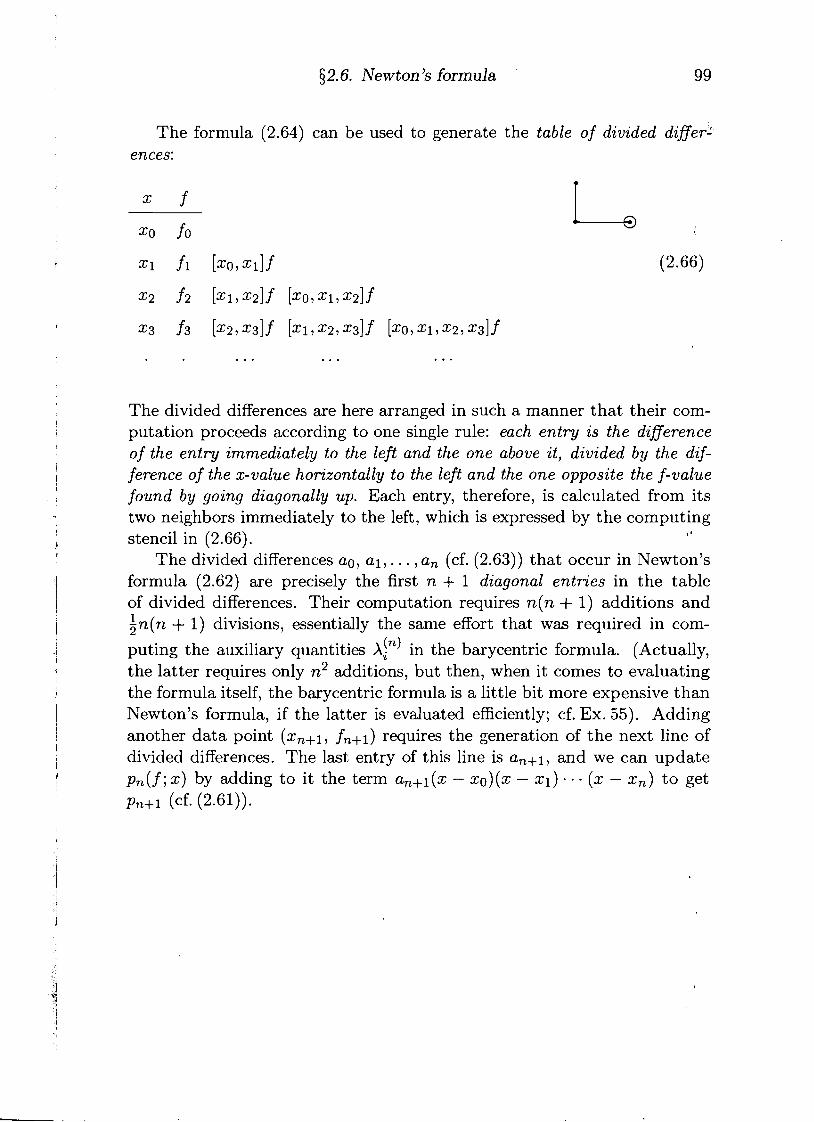
The formula (2.64) can be used to generate the table of divided differ?. ences:
The divided differences are here arranged in such a manner that their com- putation proceeds according to one single rule: each e n t r y i s the difference of the en t ry immediately to the left and the one above it, divided by the dif- ference of the x-value horizontally t o the left and the one opposite the f-value found by going diagonally up. Each entry, therefore, is calculated from its two neighbors immediately to the left, which is expressed by the computing stencil in (2.66).
The divided differences ao, a l l .. . , an (cf. (2.63)) that occur in Newton's formula (2.62) are precisely the first n + 1 diagonal entr ies in the table of divided differences. Their computation requires n(n + 1) additions and 1n(n 2 + 1) divisions, essentially the same effort that was required in com- puting the auxiliary quantities A!") in the barycentric formula. (Actually, the latter requires only n2 additions, but then, when it comes to evaluating the formula itself, the barycentric formula is a little bit more expensive than Newton's formula, if the latter is evaluated efficiently; cf. Ex. 55). Adding another data point (x,+~, fn+l) requires the generation of the next line of divided differences. The last entry of this line is an+l, and we can update p n ( f ; x) by adding to it the term U,+~(X - xo)(x - xl) . - - (x - x,) to get pn+l (cf- (2.61)).
Chapter 2. Interpolation and Approximation
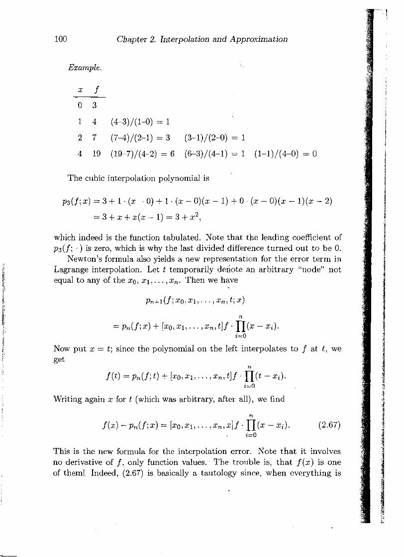
Example.
x f
The cubic interpolation polynomial is
which indeed is the function tabulated. Note that the leading coefficient of p3(f; . ) is zero, which is why the last divided difference turned out to be 0.
Newton's formula also yields a new representation for the error term in Lagrange interpolation. Let t temporarily denote an arbitrary "node" not equal to any of the xo, 21,. . . , xn. Then we have
Now put x = t; since the polynomial on the left interpolates to f at t , we
Writing again x for t (which was arbitrary, after all), we find
This is the new formula for the interpolation .error. Note that it involves no derivative of f , only function values. The trouble is, that f (x) is one of them!. Indeed, (2.67) is basically a tautology since, when everything is
$2.7. Hermite interpolation 101
written out explicitly, the formula evaporates to 0 = 0, which is correct, but *
not overly exciting. In spite of this seeming emptiness of (2.67), we can draw from it an
interesting and very useful conclusion. (For another application, see Ch. 3, Ex. 2.) Indeed, compare it with the earlier formula (2.12); one obtains
where xo, X I , . . . , x,, x are arbitrary distinct points in [a, b] and f E cn+' [a, b]. Moreover, C(x) is strictly between the smallest and largest of these points (cf. the proof of (2.12)). We can now write x = xn+l, and then replace n + 1 by n to get
Thus, for any n + 1 distinct points in [a, b] and any f E Cn[a, b], the divided diflerence off of order n is the nth scaled derivative off at some (unknown) intermediate point. If we now let all xi, i 2 1, tend to xo, then 5, being trapped between them, must also tend to s o , and, since f(") is continuous at xo, we obtain
-I
n+l times
This suggests that the nth divided diflerence at n+ 1 "confluent" (i.e., identi- cal) points be defined to be the nth derivative at this point divided by n!. This allows us, in the next section, to solve the Hermite interpolation problem.
$2.7. Hermite interpolation. The general Hermite interpolation prob- lem consists of the following: given K + 1 distinct points xo, X I , . . . , XK
in [a, b] and corresponding integers mk 2 1, and given a function f E cM-'[a, b], with M = m a mk, find a polynomial p of lowest degree such
k that, for k = 0,1 , . . . , K,
where f f ) = f(')(xk) is the pth derivative of f at xk. The problem can be thought of as a limiting case of Lagrange interp&
lation if we consider xk to be a point of multiplicity mk, that is, obtained by a confluence of mk distinct points into a single point xk. We can imag- ine setting up the table of divided differences, and Newton's interpolation
102 Chapter 2. Interpolation and Approximation
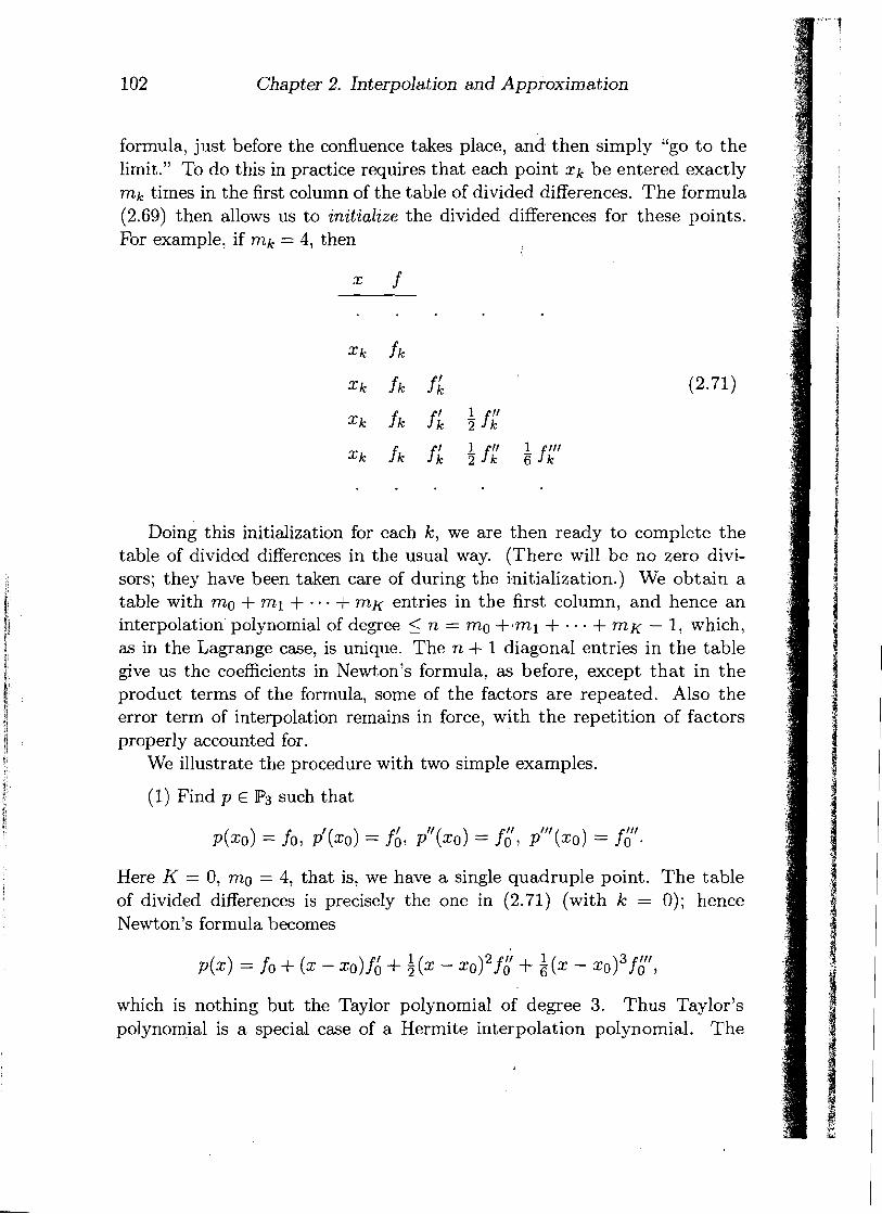
formula, just before the confluence takes place, and then simply "go to the limit." To do this in practice requires that each point x k be entered exactly mk times in the first column of the table of divided differences. The formula (2.69) then allows us to initialize the divided differences for these points. For example, if mk = 4, then
Doing this initialization for each k, we are then ready to complete the table of divided differences in the usual way. (There will be no zero divi- sors; they have been taken care of during the initialization.) We obtain a table with mo + ml + - . - + m K entries in the first column, and hence an interpolation polynomial of degree 5 n = mo +.ml + - . + m K - 1, which, as in the Lagrange case, is unique. The n + 1 diagonal entries in the table give us the coefficients in Newton's formula, as before, except that in the product terms of the formula, some of the factors are repeated. Also the error term of interpolation remains in force, with the repetition of factors properly accounted for.
We illustrate the procedure with two simple examples.
(1) Find p E P3 such that
Here K = 0, mo = 4, that is, we have a single quadruple point. The table of divided differences is precisely the one in (2.71) (with k = 0); hence Newton's formula becomes
which is nothing but the Taylor polynomial of degree 3. Thus Taylor's polynomial is a special case of a Hermite interpolation polynomial. The
$2.7. Hermite interpolation
error term of interpolation, furthermore, gives us
f (x) - p(x) = (x - xo)4 f (4) (E), E between xo and x,
which is Lagrange's form of the remainder term in Taylor's formula.
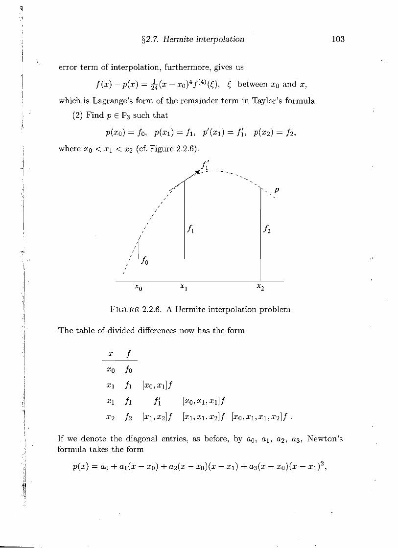
(2) Find p P3 such that
p(x0) = fo, p(x1) = fl, p'(x1) = f:, ~ ( 2 2 ) = f 2 ,
where xo < xl < x2 (cf. Figure 2.2.6)
X o 1 X2
FIGURE 2.2.6. A Hermite interpolation problem
The table of divided differences now has the form
x f
xo fo
x1 fl [xo,x11f
xl fl f; [XO, X I , ~ l ] f
~2 f 2 [xlrx2]f [ ~ 1 , ~ 1 , ~ 2 ] f [ x o , x ~ , x ~ , x ~ ] ~ .
If we denote the diagonal entries, as before, by ao, a l , a2, ag, Newton's formula takes the form
104 Chapter 2. Interpolation and Approximation
and the error formula becomes
For equally spaced points, say, xo = xl - h, x2 = ~1 + h, we have, if x = 2 1 + th, -1 5 t 5 1,
and so
with the a -norm referring to the interval [xo, x2].
s2.8. Inverse interpolation. An interesting application of interpola- tion - and, in particular, of Newton's formula - is to the solution of a nonlinear equation,
f (x) = 0. (2.72)
Here f is a given (nonlinear) function, and we are interested in a root a of the equation for which we already have two approximations,
We assume further that near the root a, the function f is monotone, so that
y = f (x) has an inverse x = f -' (l/). Denote, for short,
S(Y) = f- l(y).
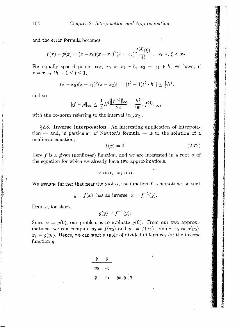
Since a = g(O), our problem is to evaluate g(0). From our two approxi- mations, we can compute yo = f (xo) and yl = f (xl), giving xo = g(yo), X I = g(yl). Hence, we can start a table of divided differences for the inverse function g:
52.8. Inverse interpolation 105
I 1
Wanting to compute g(0), we can get a first improved approximation by
i linear interpolation, I
, - I Now evaluating y2 = f (x2), we get x2 = g(y2). Hence, the table of divided I differences can be updated and becomes
Y2 x2 [ Y l , ~219 [yo, y1, y2]g .
This allows us to use quadratic interpolation to get, again with Newton's formula,
and then
Y3 = f (x3), and x3 = g(y3).
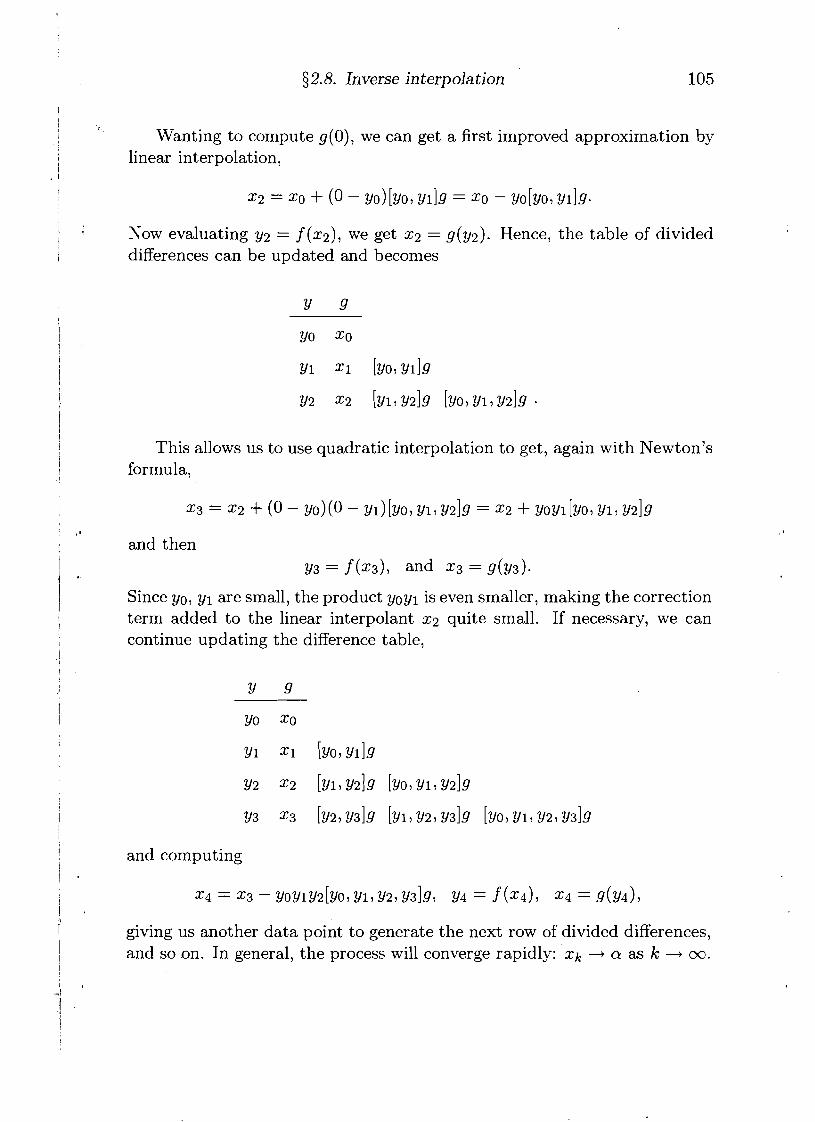
Since yo, yl are small, the product yoyl is even smaller, making the correction term added to the linear interpolant x2 quite small. If necessary, we can continue updating the difference table,
and computing
giving us another data point to generate the next row of divided differences, and so on. In general, the process will converge rapidly: xk -+ a as k --, oo.
106 Chapter 2. Interpolation and Approximation
The precise analysis of convergence, however, is not simple'.because of the complicated structure of the successive derivatives of the inverse function g = f - l .
93. Approximation and Interpolation by splinb Functions
Our concern in $2 was with approximation of functions by a single poly- nomial over a finite interval [a,b]. When more accuracy was wanted, we simply increased the degree of the polynomial, and under suitable assump- tions the approximation indeed can be made as accurate as one wishes by choosing the degree of the approximating polynomial sufficiently large.
However, there are other ways to control accuracy. One is to impose a subdivision A upon the interval [a,b],
and use low-degree polynomials on each subinterval [xi, (i = 1,2, . . . , n - 1) to approximate the given function. The rationale behind this is the recognition that on a sufficiently small interval, functions can be approxi- mated arbitrarily well by polynomials of low degree, even degree 1, or zero, for that matter. Thus, measuring the "fineness" of the subdivision A by
we try to control (increase) the accuracy by varying (decreasing) 1 A J , keeping the degrees of the polynomial pieces uniformly low.
To discuss these approximation processes, we make use of the class of functions (cf. Example (2) at the beginning of Chapter 2)
s&(A) = { s : s E c k [ a , b], sl E P,, i 1 2 n - 1 (3.3) [ ~ i r ~ i + ~ l
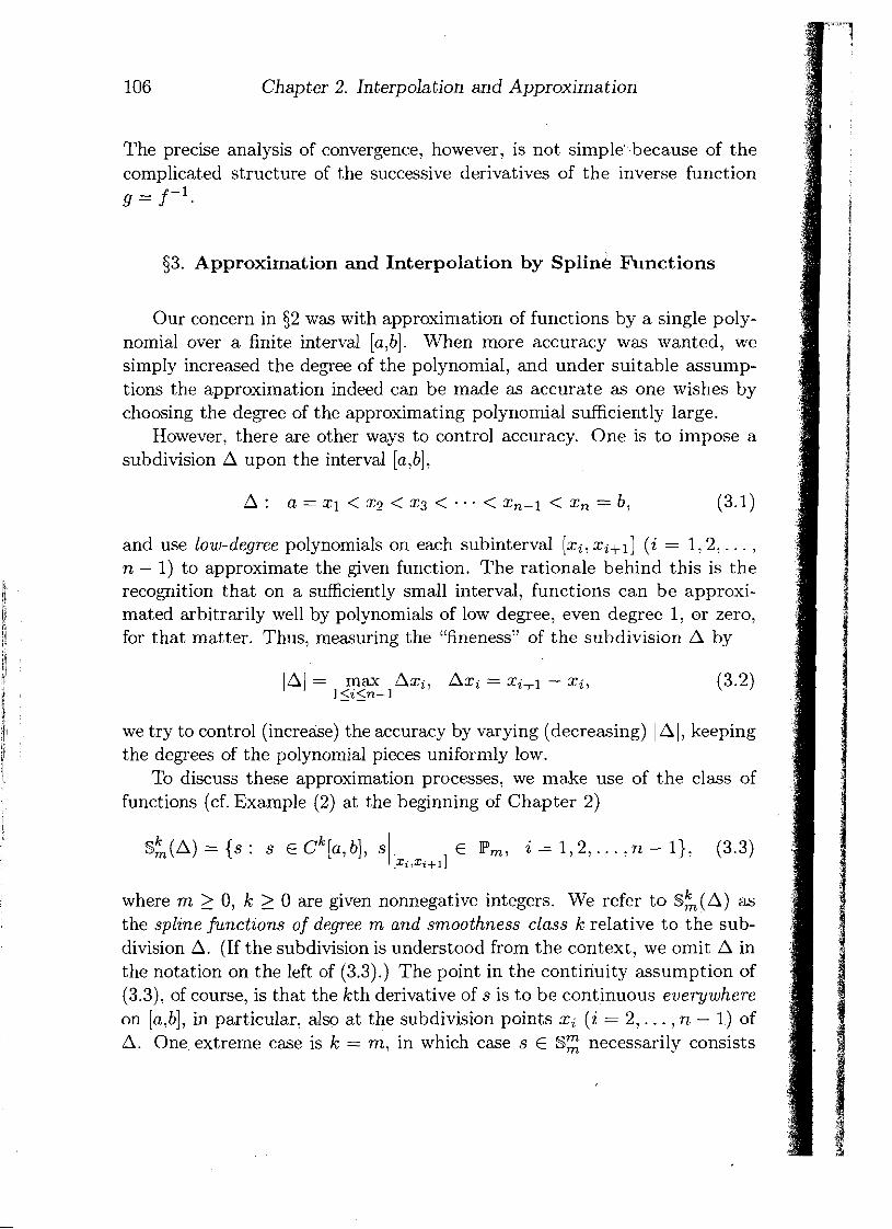
where m > 0, k > 0 are given nonnegative integers. We refer to s&(A) as the spline functions of degree rn and smoothness class k relative to the sub- division A. (If the subdivision is understood from the context, we omit A in the notation on the left of (3.3).) The point in the continuity assumption of (3.3), of course, is that the kth derivative of s is to be continuous everywhere on [a,b], in particular, also at the subdivision points xi (i = 2, . . . , n - 1) of A. One, extreme case is k = m, in which case s E S z necessarily consists
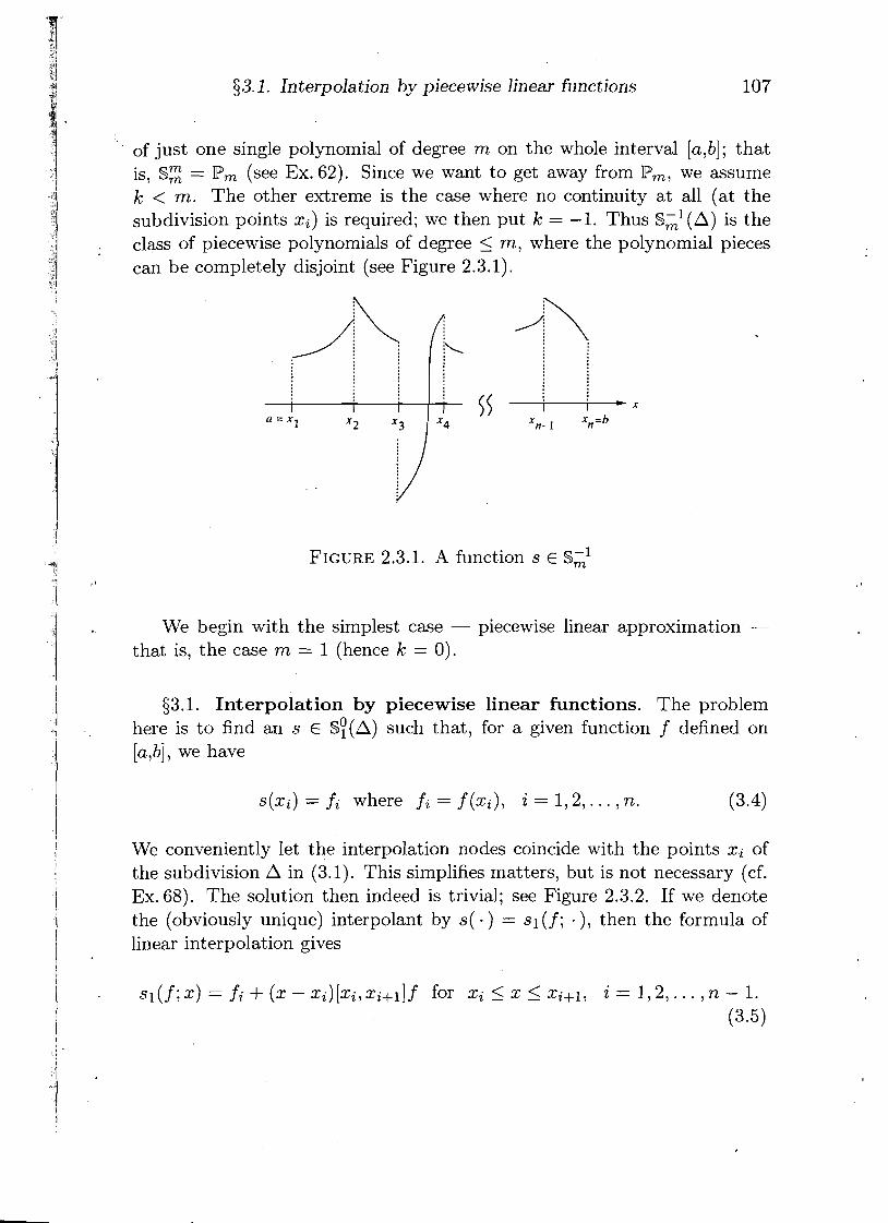
FIGURE 2.3.1. A function s E 9;'
:I , d '1 % 53.1. Interpolation by piecewise linear functions 107 8, 1 '
of just one single polynomial of degree m on the whole interval [a,b] ; that
1 is, S g = P, (see Ex. 62). Since we want to get away from P,, we assume
We begin with the simplest case - piecewise linear approximation - that is, the case m = 1 (hence k = 0).
I
g3.1. Interpolat ion by piecewise linear functions. The problem here is to find an s E s ~ ( A ) such that, for a given function f defined on [a,b], we have
k < m. The other extreme is the case where no continuity a t all (at the subdivision points xi) is required; we then put k = -1. Thus 9;' (A) is the class of piecewise polynomials of degree 5 m, where the polynomial pieces can be completely disjoint (see Figure 2.3.1).
s ( x ~ ) = fi where fi = f (xi), i = 1,2, . . . , n. (3.4)
We conveniently let the interpolation nodes coincide with the points xi of the subdivision A in (3.1). This simplifies matters, but is not necessary (cf. Ex. 68). The solution then indeed is trivial; see Figure 2.3.2. If we denote the (obviously unique) interpolant by s( . ) = sl (f ; . ), then the formula of linear interpolation gives
Chapter 2. Interpolation and Approximation
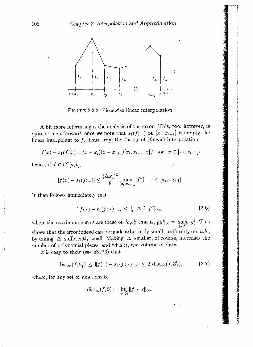
FIGURE 2.3.2. Piecewise linear interpolation
A bit more interesting is the analysis of the error. This, too, however, is quite straightforward, once we note that s l ( f ; . ) on [xi, xitl] is simply the linear interpolant to f . Thus, from the theory of (linear) interpolation,
hence, if f E c2[a, b],
If(.) - sl(f ix)I 5 max i f " ( , x E [xi, x;+l] 8 [~i,xi+~I
It then follows immediately that
where the maximum norms are those on [a,b]; that is, ((g(1, = max 191. This [a,bl
shows that the error indeed can be made arbitrarily small, uniformly on [a,b], by taking sufficiently small. Making 1 A1 smaller, of course, increases the number of polynomial pieces, and with it, the volume of data.
It is easy to show (see Ex. 73) that
where, for any set of functions S,
dist,(f,S) := inf 11 f - slim. s€S
$3.2. A basis for S? (A)
In other words, the piecewise linear interpolant sl ( f ; - ) is a nearly optimal approximation, its error differing from the error of the best approximant to f from S? by at most a factor of 2.
$3.2. A basis for s?(A). What is the dimension of the space s?(A)? In other' words, how many degrees of freedom do we have? If, for the mo- ment, we ignore the continuity requirement (i.e., if we look a t Sc1(A)), then each linear piece has 2 degrees of freedom, and there are n - 1 pieces; so dim S,'(A) = 2n - 2. Each continuity requirement imposes one equation, and hence reduces the degree of freedom by 1. Since continuity must be enforced only at the interior subdivision points xi7 i = 2 , . . . , n -- 1, we find that dim SY(A) = 2n - 2 - (n - 2) = n. SO we expect that a basis of s ~ ( A ) must consist of exactly n basis functions.
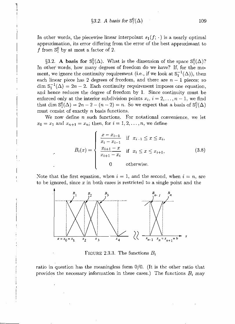
We now define n such functions. For notational convenience, we let x0 = z1 and zn+l = 2,; then, for i = 1 ,2 , . . . , n, we define
I O otherwise.
Note that the first equation, when i = 1, and the second, when i = n, are to be ignored, since z in both cases is restricted to a single point and the
FIGURE 2.3.3. The functions Bi
ratio in question has the meaningless form 010. (It is the other ratio that provides the necessary information in these cases.) The functions Bi may
110 Chapter 2. Interpolation and Approximation
be referred to as "hat functions" (Chinese hats), but note that the first and . last hat is cut in half. The functions Bi are depicted in Figure 2.3.3. We expect these functions to form a basis of s ~ ( A ) . To prove this, we must show:
(i) the functions {Bi)y==l are linearly independent; and
(ii) they span the space $)(A).
Both these properties follow from the basic fact that
which one easily reads from Figure 2.3.3. To show (i), assume there is a linear combination of the Bi that vanishes identically on [a,b],
n
S(X) = C qBi(x), S(X) 0 on [a, b]. i=l
Putting x = xj in (3.10) and using (3.9) then gives cj = 0. Since this holds for each j = 1 ,2 , . . . , n, we see that only the trivial linear combination (with all ci = 0) can vanish identically. To prove (ii), let s E S ~ ( A ) be given arbitrarily. We must show that s can be represented as a linear combination of the Bi. We claim that, indeed,
This is so, because the function on the right has the same values as s at each xj, and therefore, being in Sy(A), must coincide with s.
The formula (3.11), which holds for every s E $ ) ( A ) , may be thought of as the analogue of the Lagrange interpolation formula for polynomials. The role of the elementary Lagrange polynomials ti is now played by the Bi.
$3.3. Least squares approximation. As an application of the basis Bi we consider the problem of least squares approximation on [a,b] by functions in ( A ) . The discrete Lz approximation problem with data given a t the points xi (i = 1,2, . . . , n), of course, has the trivial solution sl ( f ; . ), which
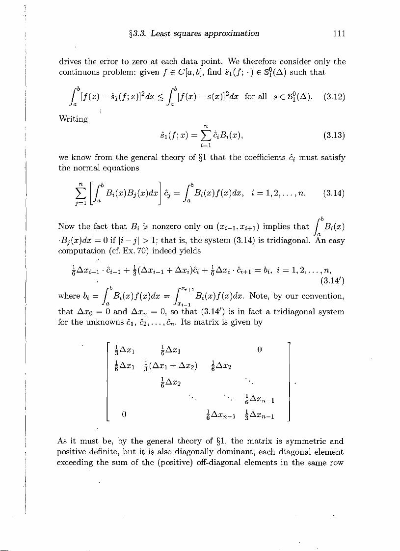
$3.3. Least squares approximation
drives the error to zero at each data point. We therefore consider only the continuous problem: given f E C [ a , b], find dl ( f ; . ) E s ~ ( A ) such that
b l b [ f ( ~ ) - ~ l ( f ; x ) ] 2 d x < ~ [f(x)-s(x)12dx for all s t s ~ ( A ) . (3.12)
Writing
we know from the general theory of $1 that the coefficients 2i must satisfy the normal equations
Now the fact that Bi is nonzero only on implies that / b ~ i ( x ) J a
.Bj (x)dx = 0 if li - j 1 > 1; that is, the system (3.14) is tridiagonal. An easy computation (cf. Ex. 70) indeed yields
f Axi-, . Ei-1 + Q ( A x ~ - ~ + Axi)& + f a x i . = bi, i = 1, 2, . . . , n, (3.14')
ib Xi+l
where bi = B ~ ( x ) f (x)dx = / Bi(x) f (x)dx. Note, by our convention, Xi-1
that Axo = 0 and Ax, = 0, so that (3.14') is in fact a tridiagonal system for the unknowns 21, E2,. . . ,En. Its matrix is given by
As it must be, by the general theory of $1, the matrix is symmetric and positive definite, but it is also diagonally dominant, each diagonal element exceeding the sum of the (positive) off-diagonal elements in the same row
112 Chapter 2. Interpolation and Approximation
by a factor of 2. The system (3.14') can therefore be solved easily, rapidly, and accurately by the Gauss elimination procedure, and there is no need for pivoting.
Like the interpolant sl (f; - ), the least squares approximant (f ; - ) , too, can be shown to be nearly optimal, in that
The spread is now by a factor of 4, rather than 2, as in (3.7).
53.4. Interpolation by cubic splines. The most widely used splines are cubic splines, in particular, cubic spline interpolants. We first discuss the interpolation problem for splines s E S;(A). Continuity of the first derivative of any cubic spline interpolant s3( f ; - ) can be enforced by prescribing the values of the first derivative at each point xi, i = 1,2, . . . , n. Thus let ml , mz,.. . , m, be arbitrary given numbers, and denote
Then we enforce s$(f; xi) = mi, i = 1,2 , . . . , n, by selecting each piece of s3(f; . ) to be the (unique) solution of a Hermite interpolation problem, namely,
We solve (3.17) by Newton's interpolation formula. The required divided differences are
$3.4. Interpolation by cubic splines
and the interpolation polynomial (in Newton's form) is
Alternatively, in Taylor's form, we can write
where, by noting that x - xi+l = x - xi - Axi,
Thus to compute s3( f; x) for any given x E [a, b] that is not an interpolation node, one first locates the interval [xi, containing x and then computes the corresponding piece (3.16) by (3.18) and (3.19).
We now discuss some possible choices of the parameters ml , m2, . . . , m,.
(i) Piecewise cubic Herrnite interpolation. Here one selects mi = f '(xi), assuming that these derivative values are known. This gives rise to a strictly local scheme, in that each piece pi can be determined independently from the others. Furthermore, the error of interpolation is easily estimated, since from the theory of interpolation,
2 2 f ( x ) - P ~ ( x ) = (X -xi) (x-xi+l) [~i,Xi,Xi+l,Xi+l, x] f , xi I x I xi+l;
hence, if f E C4 [a, b] ,
There follows
Chapter 2. Interpolation and Approximation
In the case of equally spaced points Xi , one has 1 A 1 = ( b - a)/ (n - 1) and, therefore,
I l f ( - ) - ~ d f ; . ) l l ~ = o w 4 ) as n + 00. (3.20')
This is quite satisfactory, but note that the derivative of f must be known at each point xi, and the interpolant is only in C1 [a, b].
As to the derivative values, one could approximate them by the deriva- tives of p2 ( f ; xi- 1, xi, xi+l; x) at x = xi, which requires only function values of f , except at the endpoints, where again the derivatives of f are involved, the points a = xo = xl and b = x, = x,+l being double points (cf. Ex. 71). It can be shown that this degrades the accuracy to O(lA 13) in the case of unequally spaced nodes, but maintains an O ( C ~ ) error in the case of equally spaced points.
(ii) Cubic spline interpolation. Here we require s3(f; . ) E s ~ ( A ) , that is, continuity of the second derivative. In terms of the pieces (3.16) of ss( f ; . ), this means that
and translates into a condition for the Taylor coefficients in (3.18), namely,
Plugging in the explicit values (3.19) for these coefficients, we arrive a t the linear system
where
These are n-2 linear equations in the n unknowns ml , m2,. . . , m,. Once ml and m, have been chosen in some way, the system again becomes tridiagonal in the remaining unknowns and hence is readily solved by Gauss elimination. Here are some possible choices of ml and m,.
53.5. Minimality properties of cubic spline interpolants 115
(ii.1) Complete splines: m l = ff(a) , m, = f f ( b ) . It is known that for this spline
5 1 3 where co = m, cl = %, ci = g, and c3 is a constant depending on the mesh l A i Rather remarkably, the bound for r = 0 is only five times ratio mini AZi .
larger than the bound (3.20) for the piecewise cubic Hermite interpolant, which requires derivative values of f at all interpolation nodes X i , not just at the endpoints a and b.
(ii.2) Matching of the second derivatives at the endpoints: s'3/(f; a) = f"(a), s$(f; b) = f"(b). Each of these conditions gives rise to an additional equation, namely,
One conveniently adjoins 'the first equation to the top of the system (3.22), and the second to the bottom, thereby preserving the tridiagonal structure of the system.
(ii.3) Natural cubic spline: s"(f; a ) = s"(f; b) = 0. This again produces two additional equations, which can be obtained from (3.25) by putting there f"(a) = fU(b) = 0. They are adjoined to the system (3.22) as described in (ii.2). The nice thing about this spline is that it requires only function values of f - no derivatives! - but the price one pays is a degradation of the accuracy to o ( ~ A / ~ ) near the endpoints (unless indeed f"(a) = f"(b) = 0).
(ii.4) "Not-a-knot spline" (C. de Boor): Here we require pl (x) = p2(x) and pn-2(x) -- pn-l (x); that is, the first two pieces of the spline should be the same polynomial, and similarly for the last two pieces. In effect, this means that the first interior knot 2 2 , and the last one xn-1, both are inactive (hence the name). This again gives rise to two supplementary equations expressing continuity of s$'( f ; x) at x = x2 and x = xn- 1 (cf. Ex. 72).
53.5. Minimality properties of cubic spline interpolants. The complete and natural splines defined in (ii.1) and (ii.3) of the preceding section have interesting optimality properties. To formulate them, it is
Chapter 2. Interpolation and Approximation
convenient to consider not only the subdivision A in (3.1), but also the subdivision
in which the endpoints are double knots. This means that whenever we interpolate on A', we interpolate to function values at all interior points, but to the function as well as first derivative values at the endpoints.
The first of the two theorems relates to the complete cubic spline inter- polant1 ~ c o r n p l ( f ; . )-
Theorem 2.3.1. For any functior, g E ~ ~ [ a , b] that interpolates f on A'. there holds
with equality if and only if g ( . ) = s,,,,,(f; a ) .
Note that scompl (f ; - ) in Theorem 2.3.1 also interpolates f on A', and among all such interpolants its second derivative has the smallest L2 norm.
Proof of Theorem 2.3.1. We write (for short) scOmpl = s. The theorem follows, once we have shown that
Indeed, this immediately implies (3.27), and equality in (3.27) holds if and only if g"(x) - sU(x) = 0, which, integrating twice from a to x and using the interpolation properties of s and g at x = a gives g(x) = s(x) .
To complete the proof, note that (3.28) is equivalent to
Integrating by parts, we get
lbs" (x) [g" (x) - sf' (x)] dx
b
= -l s"'(x) - s' (x)] dx,
fj 3.5. Minimality properties of cubic spline in terpolants 11 7
since s l (b ) = gl(b) = f l ( b ) , and similarly at x = a. But s"' is piecewise constant, so
f bs"'(x) [g' (x) - S' (x)] dx
since both s and g interpolate to f on A. This proves (3.29) and hence the theorem.
1 For interpolation on A, the distinction of being optimal goes to the natural cubic spline interpolant s,,, ( f ; . ). This is the content of the second theorem.
1 Theorem 2.3.2. For any fu,nction g E C2 [a, b] that interpolates f on A
I (not A'), there holds
s!
with equality if and only zf g( . ) = snat ( f ; . ).
I Putting g( ) = scorn,, ( f ; - ) in Theorem 2.3.2 immediately gives
7
Therefore, in a sense, the natural cubic spline is the "smoothest" interpolant. The property expressed in Theorem 2.3.2 is the origin of the name
The proof of Theorem 2.3.2 is virtually the same as that of Theorem 2.3.1, since (3.30) holds again, this time because s N ( b ) = sU(a) = 0.
"spline." A spline is a flexible strip of wood used in drawing curves. If its shape is given by the equation y = g(x), a 5 x 5 b, and if the spline is constrained to pass through the points (xi,gi), then it assumes a form that minimizes the bending energy
[gll (x)] dx (1 + [g1(~)12)3
over all functions g similarly constrained. For slowly varying g (llglII, << I ) , this is nearly the same as the minimum property of Theorem 2.3.2.
118 Chapter 2. Approxima tion and Interpolation
NOTES TO CHAPTER 2
There are many excellent texts on the general problem of best approximation as exemplified by (0.1). One that emphasizes uniform approximation by polynomials is.Feinerman and Newman [1974]; apart from the basic theory of best polynomial approximation, it also contains no fewer than four proofs of the fundamental the- orem of Weierstrass. For approximation in the L, and L1 norm, which is related to linear programming, a number of constructive methods, notably the Remez al- gorithms and exchange algorithms, are known, both for polynomial and rational approximation. Early, but still very readable, expositions are given in Cheney [I9661 and Rivlin [1981], and more recent accounts in Watson [I9801 and Powell [1981]. Nearly best polynomial and rational approximations are widely used in computer routines for special functions; for a survey of work in this area, up to about 1975. see Gautschi [1975a], and for subsequent work, van der Laan and Temme [I9841 and Nkmeth [1992]. Much relevant material is also contained in the books by Luke [I9751 and [1977]. The numerical approximation and software for special functions is exhaustively documented in Lozier and Olver [1994]; a recent package for some of the more esoteric functions is described in hIacLeod [1996]. For an extensive (and mathematically demanding) treatment of rational approximation, the reader is re- ferred to Petrushev and Popov [1987], and for L1 approximation, to Pinkus [1989]. Methods of nonlinear approximation, including approximation by exponential sums. i r e studied in Braess [1986]. Other basic texts on approximation and interpolation are Natanson [1964.1965,1965] and Davis [I9751 from the 1960s, and the niore re- cent books by DeVore and Lorentz [I9931 and its sequel, Lorentz, Golitschek. and Makovoz [1996]. A large variety of problems of interpolation and approximation by rational functions (including polynomials) in the complex plane is studied in iValsh [1969]. An example of a linear space containing a denumerable set of nonra- tional basis functions are the sinc functions - scaled translates of y, They are of importance in the Shannon sampling and interpolation theory (see. e.g.. Zayed [1993]) but are also useful for approximation on infinite or semi-infinite doniains in the complex plane; see Stenger [I9931 for an extensive discussion of this. A reader interested in issues of current interest related to multivariate approximation can get a good start by consulting Cheney [1986].
Rich and valuable sources on polynomials and their numerous properties of interest in applied analysis are MilovanoviC, hIitrinovid, and Rassias [I9941 and Borwein and Erdhlyi [1995]. Spline functions - in name and as a basic tool of ap- proximation - were introduced in 1946 by Schoenberg [1946]; also see Schoenberg [1973]. They have generated enormous interest, owing both to their interesting mathematical theory and practical usefulness. There are now many texts available. treating splines from various points of view. A selected list is Ahlberg. Nilson, and Walsh [1967], Niirnberger [1989], and Schumaker [I9931 for the basic theory, de Boor [I9781 and Spath [I9951 for more practical aspects including algorithms, Atteia [I9921 for an abstract treatment based on Hilbert kernels, Bartels. Beatty, and Barsky [I9871 and Dierckx [I9931 for applications to computer graphics and
Notes to Chapter 2 119
geometric modeling, and Chui [1988], de Boor, HGllig, and Riemenschneider [1993], and Bojanov, Hakopian, and Sahakian [I9931 for multivariate splines. The standard text on trigonometric series still is Zygmund [1988].
$1. Historically, the least squares principle evolved in the context of discrete linear approximation. The principle was first enunciated by Legendre in 1805 in a treatise on celestial mechanics (Legendre [1805]), although Gauss used it ear- lier in 1795, but published the method only in 1809 (in a paper also on celestial mechanics). For Gauss's subsequent treatises, published in 1821-1826, see the En- glish translation in Gauss [1995]. The statistical justification of least squares as a minimum variance (unbiased) estimator is due to Gauss. If one were to disregard pr,obabilistic arguments, then, as Gauss already remarked (Goldstine [1977, p. 212]), one could try to minimize the sum of any even (positive) power of the errors, and even let this power go to infinity, in which case one would minimize the maximum error. But by these principles " . . . we should be led into the most complicated calculations." Interestingly, Laplace a t about the same time also proposed discrete L1 approximation (under the side condition that all errors add up to zero). A reader interested in the history of least squares may wish to consult the article by Sheynin [1993].
The choice of weights wi in the discrete L2 norm ( 1 . [ I 2 , , can be motivated on statistical grounds if one assumes that the errors in the data f (xi) are uncorrelated and have zero mean and variances 4; an appropriate choice. then is wi = ac2.
The discrete problem of minimizing J J f - cp112., over functions cp in as given by (0.2) can be rephrased in terms of an overdetermined system of linear equations, PC = f , where P = [rj(xi)] is a rectangular matrix of size N x n, and f = [f (xi)] the data vector of dimension N. If r = f - PC, r = [ri] denotes the residual vector, one tries to find the coefficient vector c E Rn such that xi wir? is as small as possible. There is a vast literature dealing with overdetermined systems involving more general (full or sparse) matrices and their solution by the method of least squares. A large arsenal of modern techniques of matrix computation can be brought to bear on this problem; see, for example, Bjorck [I9961 for an extensive discussion. In the special case considered here, the method of (discrete) orthogonal polynomials, however, is more efficient. It has its origin in the work of Chebyshev [1859]; a contemporary exposition, including computational and statistical issues, is given in Forsythe [1957].
There are interesting variations on the theme of polynomial least squares ap- proximation. One is to minimize ( 1 f - p(12.dX among all polynomials in p, subject to interpolatory constraints a t m + 1 given points, where m < n. It turns out that this can be reduced to an unconstrained least squares problem, but for a different measure dX and a different function f ; cf. Gautschi [1996,§2.I]. Something similar is true for approximation by rational functions with a prescribed denominator polyno- mial. A more substantial variation obtains if one wants to approximate simultane- ously a function f and its first s derivatives. In the most general setting, this would require the minimization of S, xt=, [ f (01 (t) - p(u) (t)12dX, ( t ) among all polynomi-
120 Chapter 2. Approximation and Interpolation
als p E P,, where dX, are given (continuous or discrete) positive measures. The problem can be solved, as in 51.2, by orthogonal polynomials, but they are now or- thogonal with respect to the inner product (u, v ) ~ , = C:=o JR U(O) ( t ) v ( ~ ) ( t ) d ~ , (t ) - a so-called Sobolev inner product. This gives rise to Sobolev orthogonal poly- nomials; see Gautschi [1996,§2.2] for some history on this problem and relevant literature.
51.2. The alternative form (1.15') of computing the coefficients ej was suggested in the 1972 edition of Conte and de Boor 119801 and is further discussed by Shampine [1975]. The Gram-Schmidt procedure described at the end of this section is now called the classical Gram-Schmidt procedure. There are other, modified, versions of Gram-Schmidt that are computationally more effective; see, for example, Bjorck [1996,pp. 61ffl.
51.4. The standard text on Fourier series, as already mentioned, is Zygmund 119881, and on orthogonal polynomials, Szego 119751. Not only is it true that orthog- onal polynomials satisfy a three-term recurrence relation (1.26): but the converse is also true: any system {nk) of monic polynomials satisfying (1.26) for all k 2 0, with real coefficients rrk and Pk > 0, is necessarily orthogonal with respect to some (in general unknown) positive measure. This is known as Favard's Theorem (cf., e.g., Natanson 11965, Vol. 2, Ch. 8, $61. The computation of orthogonal polynomi- als, when the recursion coefficients are not known explicitly, is not an easy task; a number of methods are surveyed in Gautschi [1996]. Orthogonal systems in L2(R) that have become prominent in recent years are wavelets, which are functions of the foim +j,k(t) = 2jI2+(2jt - k) , j , k = 0, f l , f 2,. . . , with + a "mother wavelet" - square integrable on R and (usually) satisfying JR @(t)dt = 0. Among the grow- ing textbook and monograph literature on this subject, we mention Chui [1992], Daubechies [1992], Walter [1994], Wickerhauser [1994], and Resni koff and Wells [1997].
52. Although interpolation by polynomials and spline fuilctions is most com- mon, it is sometimes appropriate to use other systems of approximants for interpo- lation, for example, trigonometric polynomials or rational functions. Trigonometric interpolation at equally spaced points is closely related to discrete Fourier analysis and hence accessible to the Fast Fourier Transform (FFT). For this, and also for rational interpolation algorithms, see, for example, Stoer and Bulirsch 11993, 552.2 and 2.31. For the fast Fourier transform and some of its important applications, see Henrici [1979a] and Van Loan [1992].
Besides Lagrange and Hermite interpolation, other types of interpolation processes have been studied in the literature. Among these are Fejkr-Hermite in- terpolation, where one interpolates to given function values and zero values of the derivative, and Birkhoff (also called lacunary) interpolation, which is similar to Her- mite interpolation, but derivatives of only preselected orders are being interpolated. Remarkably, Fejkr-Hermite interpolation at the Chebyshev points (defined in 52.4) converges for .every continuous function f E C[-1, 11. The convergence theory of
Notes to Chapter 2 121
Lagrange and Fej6r-Hermite interpolation is the subject of a monograph by Szaba- dos and Vdrtesi [1990]. The most comprehensive work on Birkhoff interpolation is the book by G. G. Lorentz, Jetter, and Riemenschneider [1983]. A more recent monograph by R. A. Lorentz [I9921 deals with multivariate Birkhoff interpolation.
$2.1. The growth of the Lebesgue constants A, is at least O(1ogn) as n --t oo; specifically, A,' > ? logn + c for any triangular array of interpolation nodes (cf. $2.3), where the constant c can be expressed in terms of Euler's constant y (cf. Ch. 1.; Mach. Ass. 4) by c = 1 (log + y) = .9625228. . . ; see Rivlin [1990, Thm. 1.21. The Chebyshev points achieve the optimal order O(1og n); for them, A, 5 $ log n + l (Rivlin [1990, Thm. 1.21). Equally spaced nodes, on the other hand, lead to exponen- tial growth of the Lebesgue constants inasmuch as A, - 2,+l/(en logn) for n --t oo; see Trefethen and Weideman [1991] for some history on this result and Brutman [1997a] for a recent survey on Lebesgue constants. The very last statement of $2.1 is the content of Faber's Theorem (see, e.g., Natanson [1965, Vol. 3, Ch. 2, Thm. 2]), which says that, no matter how one chooses the triangular array of nodes (2.16) in [a, b], there is always a continuous function f E C[a, b] for which the Lagrange inter- polation process does not converge uniformly to f . Indeed, there is an f E C[a, b] for which Lagrange interpolation diverges almost everywhere in [a, b]; see Erdos and Vkrtesi [1980]. Compare this with Fejdr-Hermite interpolation.
52.3. A more complete discussion of how the convergence domain of Lagrange interpolation ip the complex plane depends on the limit distribution of the inter- polation nodes can be found in Krylov [1962, Ch. 12, $21.
Runge's example is further elucidated in Epperson [1987]. For an analysis of Bernstein's ' example, we refer to Natanson [1965, Vol. 3, Ch. 2, $21. The same divergence phenomenon, incidentally, is exhibited also for a large class of nonequally spaced nodes; see Brutman and Passow [1995]. The proof of Example (5) follows Fejdr [1918].
$2.4. The Chebyshev polynomial arguably is one of the most interesting poly- nomials from the point of view not only of approximation theory, but also of algebra and number theory. In Rivlin's words, it " . . . is like a fine jewel that reveals differ- ent characteristics under illumination from various positions." In his text, Rivlin [I9901 gives ample testimony in support of this view. Another text, unfortunately available only in Russian (or Polish), is Paszkowski [1983], which has an exhaus- tive account of analytic properties of Chebyshev polynomials as well as numerical applications.
The convergence result stated in (2.49) follows from (2.11) and the logarithmic growth of A,, since En ( f ) log n --t 0 for f E C1 [-I, 111 by Jackson's theorems (cf. Cheney [1966, p. 1471). A more precise estimate for the error in (2.54) is En ( f ) 5
< (4 + $ log n) E,(f) (Rivlin [199O, Thm. 3.3]), where the infinity norm 117,-f Ilm - refers to the interval [-I, 11 and En( f ) is the best uniform approximation of f by polynomials of degree n.
$2.5. T h e algorithm (2.59) for calculating the auxiliary quantities A!") in the
Chapter 2. Approximation and Interpolation
barycentric formula is due to Werner [1984]. Scaling and translating the nodes x ( ~ )
will not affect the numerical properties of the algorithm, since the quantities $ , which control cancellation, are invariant with respect to any linear transformation of the nodes. Ordering of the nodes, however, does, as was noted experimentally by Werner and also confirmed in Gautschi [1997,53.1.] in connection with the cal- . culation of Cotes numbers (for Newton-Cotes integration).
Barycentric formulae have been developed also for trigonometric interpolation (see Henrici [1979b] for uniform, and Salzer [I9491 and Berrut [I9841 for nonuniform, distributions of the nodes), and for cardinal (sinc-) interpolation (Berrut [1989]).
32.7. There are explicit formulae, analogous to Lagrange's formula, for Her- mite interpolation in the most general case; see, for example, Stoer and Bulirsch [1993,32.1.5]. For the important special case rnk = 2, see also Ch. 3, Ex. 33.
32.8. To estimate the error for inverse interpolation, using an appropriate ver- sion of (2.12), one needs the derivatives of the inverse function f -'. A general expression for the nth derivative of f- ' in terms of the first n derivatives of f is derived in Ostrowski [1973, Appendix C] .
53. The definition of the class of spline functions S i ( A ) can be refined to s ~ ( A ) , where kT = [kZ, kg, . . . , kn-l] is a vector with integer components ki 2 -1 specifying the degree of smoothness a t the interior knots xi; that is, s ( j ) (xi + 0) - s(j)(xi - 0) = 0 for j = 0,1, . . . , ki. Then S& (A) as defined in (3.3) becomes S: (A)
"
with k = [k, k , . . . , k].
53.1. As simple as the procedure of piecewise linear interpolation may seem, it can be applied to advantage in numerical Fourier analysis, for example. In trying to compute the (complex) Fourier coefficients cn(f) = & J:" f ( ~ ) e - ~ ~ ~ d x of a 2n-periodic function f , one often approximates them by the "discrete Fourier
N-1 transform'' En(f) = k C k = o f ( ~ ~ ) e - " ~ ~ , where xk = k 3 . This can be computed efficiently (for large N ) by the Fast Fourier Transform. Note, however, that en( f ) is periodic in n with period N , whereas the true Fourier coefficients cn( f ) tend to zero as n --t oo. To remove this deficiency, one can approximate f by some (simple) function q and thereby approximate cn( f ) by cn (q). Then cn ( y ) will indeed tend to zero as n 4 co. The simplest choice for y is precisely the piecewise linear interpolant y = sl( f ; . ) (relative to the uniform partition of [O, 2x1 into N subintervals). One then finds, rather remarkably (see Ch. 3, Ex. 13), that cn(y) is a multiple of the discrete Fourier transform, namely, cn( f ) = rnEn(f ), where rn =
sin(nx/N) 2
( nn/N ) ; this still allows the application of the FFT but corrects the behavior
of En( f ) at infinity. The same modification of the discrete Fourier transform by an ,
"attenuation factor" rn occurs for many other approximation processes f = 9; see Gautschi [1971/ 19721 for a general theory (and history) of attenuation factors.
The near optimality of the piecewise linear interpolant sl ( f ; . ), as expressed by the inequalities in (3.7), is noted by de Boor [1978, pp. 40-411.
Notes to Chapter 2
$3.2. The basi's (3.8) for Sy(A) is a special case of a B-spline basis that can be defined for any space of spline functions S k ( A ) previously introduced (cf. de Boor [1978, Thm. 9.11. The B-splines are formed by means of divided differences of order m + 1 applied to the truncated power (t - x)? (considered as a function of t). Like the basis in (3.8), each basis function of a B-spline basis is supported on at most m + 1 consecutive intervals of A and is positive on the interior of the support.
$3.3. A proof of the near optimality of the piecewise linear least squares ap- proximant il ( f ; e ), as expressed by the inequalities (3.15), can be found in de Boor [1978, pp. 41-44]. For smoothing and least squares approximation procedures involving cubic splines, see, for example, de Boor [1978, Ch. 141.
$3.4. (i) For the remark in the last paragraph of (i), see de Boor [1978, Ch. 4, Problems 3 and 41.
(ii.1) The error bounds in (3.24), which for T = 0 and T = 1 are asymptotically sharp, are due to Hall and Meyer [1976].
(ii.2) The cubic spline interpolant matching second derivatives at the endpoints 3 satisfies the same error bounds as in (3.24) for r = 0, 1, 2, with constants co = =,
cl = 6 and c2 = $; see Kershaw [197l,Thm. 21. The same is shown also for periodic spline interpolants s, satisfying s(')(a) = s(')(b) for T = 0, 1, 2.
(ii.3) Even though the natural spline interpolant, in general, converges only with order lAI2 (e.g., for uniform partitions A), it has been shown by Atkinson [I9681 that the order "of convergence is )AI4 on any compact interval contained in the open interval (a, b), and by Kershaw [I9711 even on intervals extending (in a sense made precise) to [a, b] as IAl + 0. On such intervals, in fact, the natural spline interpolant s provides approximations to any f E C4[a, b] with errors satisfying
1 1 \ I f ( ' ) - S ( ~ ) ~ I , < ~ C , K A ~ - ~ , where K = 2 + $ 1 1 f ( 4 ) 1 / , and co = g , cl = 1 and C2 = 1.
(ii.4) The error of the "not-a-knot" spline interpolant is of the same order as the error of the complete spline; it follows from Beatson [1986, Eq. (2.1)] that for func- tions f E C4[a,b], one has 1 1 f(') - s(')l, < ~ ~ l ~ 1 ~ - ~ l l f ( 4 ) ) 1 0 = , T = 0, 1, 2 (at least when n 2 6), where c, are constants independent of f and A. The same bounds are valid for other schemes that depend only on function values, for example, the scheme with ml equal to the first (or second) derivative of p3 ( f ; X I , x2,x3,24; . ) at x = a, and similarly for m,. The first of' these schemes (using first-order deriva- tives of p3) is in fact the one recommended by Beatson and Chacko [1989], [I9921 for general-purpose interpolation. Numerical experiments in Beatson and Chacko [I9891 suggest values of approximately 1 for the constants c, in the preceding er- ror estimates. In Beatson and Chacko [I9921 further comparisons are made among many other cubic spline interpolation schemes.
$3.5. The minimum norm property of natural splines (Theorem 2.3.1) and its proof based on the identity (3.28), called "the first integral relation" in Ahlberg, Nilson, and Walsh [1967], is due to Holladay [1957], who derived it in the context of numerical quadrature. "Much of the present-day theory of splines began with this
124 Chap t er 2. Approxima tion and Interpolation
theorem" (Ahlberg, Nilson, and Walsh [1967,p. 31). An elegant alternative proof of (3.29), and hence of the theorem, can be based (cf. de Boor [1978, pp. 64-66]) on the Peano representation (see Ch. 3,523) of the second divided difference of g - s, that is, [xi-- xi, ~ ~ + ~ ] ( g - S) = S, K (t) (g"(t) - sU(t))dt, by noting that the Peano kernel K, up to a constant, is the B-spline Bi defined in (3.8). Since the left-hand side is zero by the interpolation properties of g and s, it follows from the preceding equation that g" - s" is orthogonal to the span of the Bi, hence to s", which lies in this span.