Embed Size (px)
DESCRIPTION
Chapter 3. Demand Forecasting. Introduction . Demand estimates for products and services are the starting point for all the other planning in operations management. Management teams develop sales forecasts based in part on demand estimates. - PowerPoint PPT Presentation
Citation preview
1
Chapter 3
Demand Forecasting

2
Introduction
Demand estimates for products and services are the starting point for all the other planning in operations management.
Management teams develop sales forecasts based in part on demand estimates.
The sales forecasts become inputs to both business strategy and production resource forecasts.

3
Forecasting is an Integral Part of Business Planning
ForecastMethod(s)
DemandEstimates
SalesForecast
ManagementTeam
Inputs:Market,
Economic,Other
BusinessStrategy
Production ResourceForecasts
4
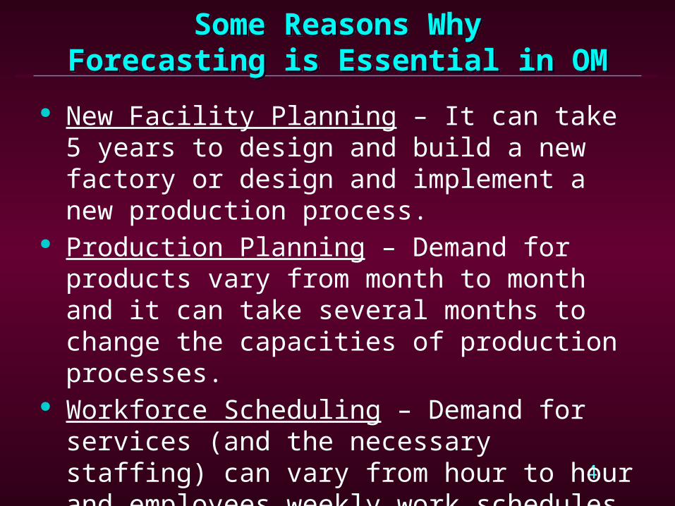
Some Reasons WhyForecasting is Essential in OM
New Facility Planning – It can take 5 years to design and build a new factory or design and implement a new production process.
Production Planning – Demand for products vary from month to month and it can take several months to change the capacities of production processes.
Workforce Scheduling – Demand for services (and the necessary staffing) can vary from hour to hour and employees weekly work schedules must be developed in advance.

5
Examples of Production Resource Forecasts
LongRange
MediumRange
ShortRange
Years
Months
Days,Weeks
Product Lines,Factory Capacities
ForecastHorizon
TimeSpan
Item BeingForecasted
Unit ofMeasure
Product Groups,Depart. Capacities
Specific Products,Machine Capacities
Dollars,Tons
Units,Pounds
Units,Hours

6
Forecasting Methods
Qualitative Approaches Quantitative Approaches
7
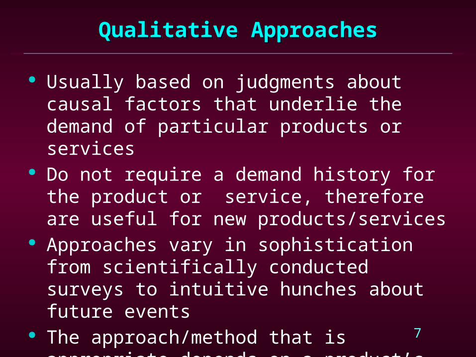
Qualitative Approaches
Usually based on judgments about causal factors that underlie the demand of particular products or services
Do not require a demand history for the product or service, therefore are useful for new products/services
Approaches vary in sophistication from scientifically conducted surveys to intuitive hunches about future events
The approach/method that is appropriate depends on a product’s life cycle stage

8
Qualitative Methods
Educated guess intuitive hunches Executive committee consensus Delphi method Survey of sales force Survey of customers Historical analogy Market research scientifically conducted
surveys

9
Quantitative Forecasting Approaches
Based on the assumption that the “forces” that generated the past demand will generate the future demand, i.e., history will tend to repeat itself
Analysis of the past demand pattern provides a good basis for forecasting future demand
Majority of quantitative approaches fall in the category of time series analysis
10
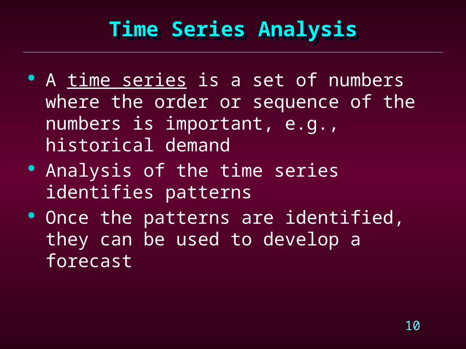
A time series is a set of numbers where the order or sequence of the numbers is important, e.g., historical demand
Analysis of the time series identifies patterns Once the patterns are identified, they can be used to
develop a forecast
Time Series Analysis

11
Components of a Time Series
Trends are noted by an upward or downward sloping line.
Cycle is a data pattern that may cover several years before it repeats itself.
Seasonality is a data pattern that repeats itself over the period of one year or less.
Random fluctuation (noise) results from random variation or unexplained causes.

12
Seasonal Patterns
Length of Time Number of Before Pattern Length of Seasons Is Repeated Season in Pattern
Year Quarter 4 Year Month 12 Year Week 52 Month Day 28-31 Week Day 7

13
Quantitative Forecasting Approaches
Linear Regression Simple Moving Average Weighted Moving Average Exponential Smoothing (exponentially weighted
moving average) Exponential Smoothing with Trend (double
exponential smoothing)

14
Long-Range Forecasts
Time spans usually greater than one year Necessary to support strategic decisions about
planning products, processes, and facilities
15
Simple Linear Regression
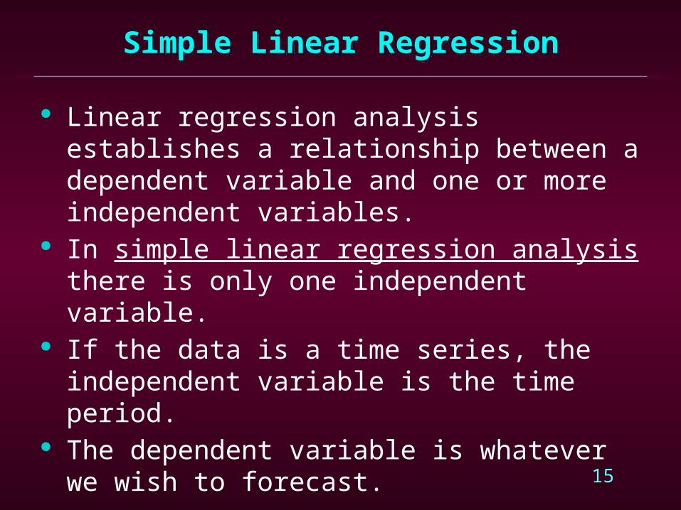
Linear regression analysis establishes a relationship between a dependent variable and one or more independent variables.
In simple linear regression analysis there is only one independent variable.
If the data is a time series, the independent variable is the time period.
The dependent variable is whatever we wish to forecast.
16
Simple Linear Regression
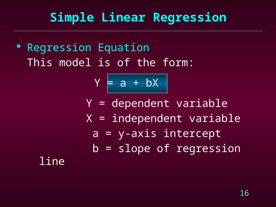
Regression EquationThis model is of the form:
Y = a + bX
Y = dependent variable X = independent variable
a = y-axis intercept b = slope of regression line

17
Simple Linear Regression
Constants a and bThe constants a and b are computed using the following equations:
2
2 2x y- x xya = n x -( x)
2 2xy- x yb = n x -( x)
n

18
Simple Linear Regression
Once the a and b values are computed, a future value of X can be entered into the regression equation and a corresponding value of Y (the forecast) can be calculated.

19
Example: College Enrollment
Simple Linear RegressionAt a small regional college enrollments have
grown steadily over the past six years, as evidenced below. Use time series regression to forecast the student enrollments for the next three years.
Students StudentsYear Enrolled (1000s) Year Enrolled (1000s) 1 2.5 4 3.2 2 2.8 5 3.3 3 2.9 6 3.4

20
Example: College Enrollment
Simple Linear Regression
x y x2 xy1 2.5 1 2.52 2.8 4 5.63 2.9 9 8.74 3.2 16 12.85 3.3 25 16.56 3.4 36 20.4 Sx=21 Sy=18.1 Sx2=91 Sxy=66.5

21
Example: College Enrollment
Simple Linear Regression
Y = 2.387 + 0.180X
291(18.1) 21(66.5) 2.3876(91) (21)a
6(66.5) 21(18.1) 0.180105b
22
Example: College Enrollment
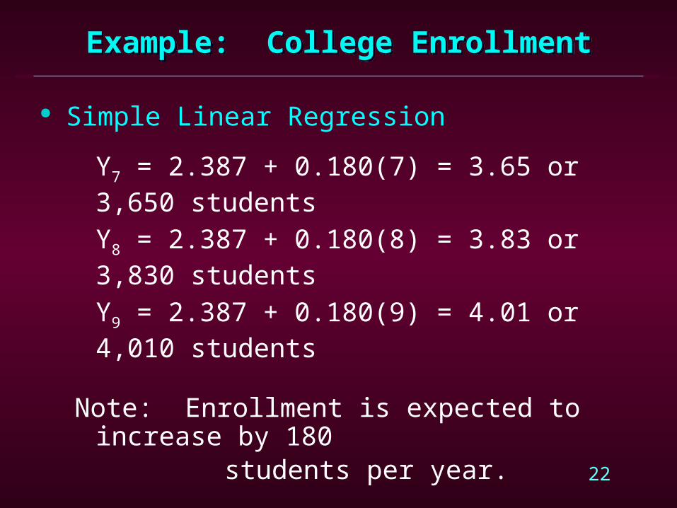
Simple Linear Regression
Y7 = 2.387 + 0.180(7) = 3.65 or 3,650 students Y8 = 2.387 + 0.180(8) = 3.83 or 3,830 students
Y9 = 2.387 + 0.180(9) = 4.01 or 4,010 students
Note: Enrollment is expected to increase by 180 students per year.

23
Simple Linear Regression
Simple linear regression can also be used when the independent variable X represents a variable other than time.
In this case, linear regression is representative of a class of forecasting models called causal forecasting models.

24
Example: Railroad Products Co.
Simple Linear Regression – Causal ModelThe manager of RPC wants to project the
firm’s sales for the next 3 years. He knows that RPC’s long-range sales are tied very closely to national freight car loadings. On the next slide are 7 years of relevant historical data.
Develop a simple linear regression model between RPC sales and national freight car loadings. Forecast RPC sales for the next 3 years, given that the rail industry estimates car loadings of 250, 270, and 300 million.

25
Example: Railroad Products Co.
Simple Linear Regression – Causal Model
RPC Sales Car LoadingsYear ($millions) (millions)1 9.5 1202 11.0 1353 12.0 1304 12.5 1505 14.0 1706 16.0 1907 18.0 220

26
Example: Railroad Products Co.
Simple Linear Regression – Causal Model
x y x2 xy
120 9.5 14,400 1,140135 11.0 18,225 1,485130 12.0 16,900 1,560150 12.5 22,500 1,875170 14.0 28,900 2,380190 16.0 36,100 3,040220 18.0 48,400 3,960
1,115 93.0 185,425 15,440

27
Example: Railroad Products Co.
Simple Linear Regression – Causal Model
Y = 0.528 + 0.0801X
2185,425(93) 1,115(15,440)a 0.5287(185,425) (1,115)
27(15,440) 1,115(93)b 0.08017(185,425) (1,115)

28
Example: Railroad Products Co.
Simple Linear Regression – Causal Model
Y8 = 0.528 + 0.0801(250) = $20.55 million Y9 = 0.528 + 0.0801(270) = $22.16 million
Y10 = 0.528 + 0.0801(300) = $24.56 million
Note: RPC sales are expected to increase by $80,100 for each additional million national freight car loadings.

29
Multiple Regression Analysis
Multiple regression analysis is used when there are two or more independent variables.
An example of a multiple regression equation is:
Y = 50.0 + 0.05X1 + 0.10X2 – 0.03X3
where: Y = firm’s annual sales ($millions) X1 = industry sales ($millions) X2 = regional per capita income
($thousands) X3 = regional per capita debt ($thousands)
30
Coefficient of Correlation (r)
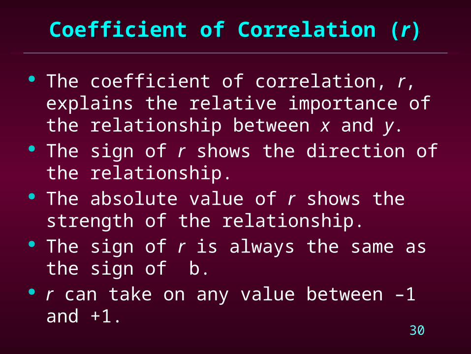
The coefficient of correlation, r, explains the relative importance of the relationship between x and y.
The sign of r shows the direction of the relationship. The absolute value of r shows the strength of the
relationship. The sign of r is always the same as the sign of b. r can take on any value between –1 and +1.
31
Coefficient of Correlation (r)
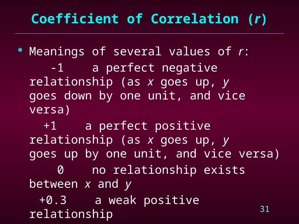
Meanings of several values of r: -1 a perfect negative relationship (as x goes up, y
goes down by one unit, and vice versa) +1 a perfect positive relationship (as x goes up, y
goes up by one unit, and vice versa) 0 no relationship exists between x and y
+0.3 a weak positive relationship -0.8 a strong negative relationship

32
Coefficient of Correlation (r)
r is computed by:
2 2 2 2( ) ( )n xy x y
rn x x n y y

33
Coefficient of Determination (r2)
The coefficient of determination, r2, is the square of the coefficient of correlation.
The modification of r to r2 allows us to shift from subjective measures of relationship to a more specific measure.
r2 is determined by the ratio of explained variation to total variation:
22
2( )( )Y y
ry y

34
Example: Railroad Products Co.
Coefficient of Correlation
x y x2 xy y2
120 9.5 14,400 1,140 90.25135 11.0 18,225 1,485 121.00130 12.0 16,900 1,560 144.00150 12.5 22,500 1,875 156.25170 14.0 28,900 2,380 196.00190 16.0 36,100 3,040 256.00220 18.0 48,400 3,960 324.00
1,115 93.0 185,425 15,440 1,287.50

35
Example: Railroad Products Co.
Coefficient of Correlation
r = .9829
2 2
7(15,440) 1,115(93)7(185,425) (1,115) 7(1,287.5) (93)
r
36
Example: Railroad Products Co.
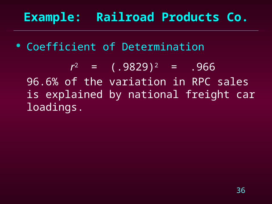
Coefficient of Determination
r2 = (.9829)2 = .96696.6% of the variation in RPC sales is explained by national freight car loadings.
37
Ranging Forecasts
Forecasts for future periods are only estimates and are subject to error.
One way to deal with uncertainty is to develop best-estimate forecasts and the ranges within which the actual data are likely to fall.
The ranges of a forecast are defined by the upper and lower limits of a confidence interval.
38
Seasonalized Time Series Regression Analysis
Select a representative historical data set. Develop a seasonal index for each season. Use the seasonal indexes to deseasonalize the data. Perform lin. regr. analysis on the deseasonalized data. Use the regression equation to compute the forecasts. Use the seas. indexes to reapply the seasonal patterns
to the forecasts.

39
Example: Computer Products Corp.
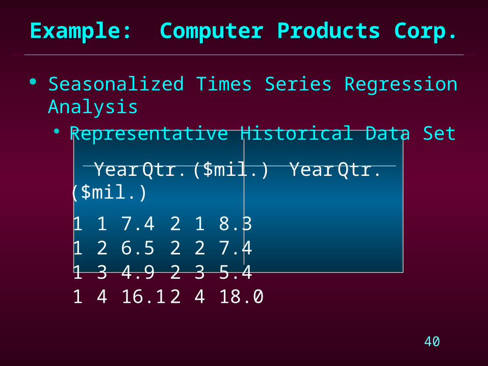
Seasonalized Times Series Regression AnalysisAn analyst at CPC wants to develop next year’s
quarterly forecasts of sales revenue for CPC’s line of Epsilon Computers. She believes that the most recent 8 quarters of sales (shown on the next slide) are representative of next year’s sales.
40
Example: Computer Products Corp.
Seasonalized Times Series Regression Analysis Representative Historical Data Set
Year Qtr. ($mil.) Year Qtr.($mil.)
1 1 7.4 2 1 8.31 2 6.5 2 2 7.41 3 4.9 2 3 5.41 4 16.1 2 4 18.0
41
Example: Computer Products Corp.
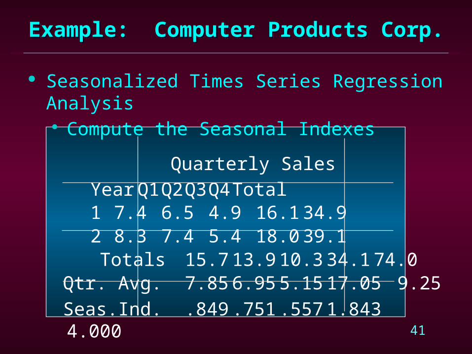
Seasonalized Times Series Regression Analysis Compute the Seasonal Indexes
Quarterly SalesYear Q1 Q2 Q3 Q4 Total1 7.4 6.5 4.9 16.1 34.92 8.3 7.4 5.4 18.0 39.1
Totals 15.7 13.9 10.3 34.1 74.0 Qtr. Avg. 7.85 6.95 5.15 17.05 9.25 Seas.Ind. .849 .751 .557 1.843 4.000

42
Example: Computer Products Corp.
Seasonalized Times Series Regression Analysis Deseasonalize the Data
Quarterly SalesYear Q1 Q2 Q3 Q41 8.72 8.66 8.80 8.742 9.78 9.85 9.69 9.77

43
Example: Computer Products Corp.
Seasonalized Times Series Regression Analysis Perform Regression on Deseasonalized Data
Yr. Qtr. x y x2 xy1 1 1 8.72 1 8.721 2 2 8.66 4 17.321 3 3 8.80 9 26.401 4 4 8.74 16 34.962 1 5 9.78 25 48.902 2 6 9.85 36 59.102 3 7 9.69 49 67.832 4 8 9.77 64 78.16
Totals 36 74.01 204 341.39

44
Example: Computer Products Corp.
Seasonalized Times Series Regression Analysis Perform Regression on Deseasonalized Data
Y = 8.357 + 0.199X
2204(74.01) 36(341.39)a 8.3578(204) (36)
28(341.39) 36(74.01)b 0.1998(204) (36)

45
Example: Computer Products Corp.
Seasonalized Times Series Regression Analysis Compute the Deseasonalized Forecasts
Y9 = 8.357 + 0.199(9) = 10.148 Y10 = 8.357 + 0.199(10) = 10.347
Y11 = 8.357 + 0.199(11) = 10.546 Y12 = 8.357 + 0.199(12) = 10.745
Note: Average sales are expected to increase by .199 million (about $200,000) per
quarter.

46
Example: Computer Products Corp.
Seasonalized Times Series Regression Analysis Seasonalize the Forecasts
Seas. Deseas. Seas.Yr. Qtr. Index Forecast Forecast
3 1 .849 10.148 8.623 2 .751 10.347 7.773 3 .557 10.546 5.873 4 1.843 10.745 19.80
47
Short-Range Forecasts
Time spans ranging from a few days to a few weeks Cycles, seasonality, and trend may have little effect Random fluctuation is main data component

48
Evaluating Forecast-Model Performance
Short-range forecasting models are evaluated on the basis of three characteristics:
Impulse response Noise-dampening ability Accuracy
49
Evaluating Forecast-Model Performance
Impulse Response and Noise-Dampening Ability If forecasts have little period-to-period fluctuation,
they are said to be noise dampening. Forecasts that respond quickly to changes in data
are said to have a high impulse response. A forecast system that responds quickly to data
changes necessarily picks up a great deal of random fluctuation (noise).
Hence, there is a trade-off between high impulse response and high noise dampening.

50
Evaluating Forecast-Model Performance
Accuracy Accuracy is the typical criterion for judging the
performance of a forecasting approach Accuracy is how well the forecasted values match
the actual values

51
Monitoring Accuracy
Accuracy of a forecasting approach needs to be monitored to assess the confidence you can have in its forecasts and changes in the market may require reevaluation of the approach
Accuracy can be measured in several ways Standard error of the forecast (covered earlier) Mean absolute deviation (MAD) Mean squared error (MSE)

52
Monitoring Accuracy
Mean Absolute Deviation (MAD)
nperiodsn for deviation absolute of Sum=MAD
n
i ii=1
Actual demand -Forecast demandMAD = n

53
Mean Squared Error (MSE)
MSE = (Syx)2
A small value for Syx means data points are tightly grouped around the line and error range is small.
When the forecast errors are normally distributed, the values of MAD and syx are related:
MSE = 1.25(MAD)
Monitoring Accuracy

54
Short-Range Forecasting Methods
(Simple) Moving Average Weighted Moving Average Exponential Smoothing Exponential Smoothing with Trend
55
Simple Moving Average
An averaging period (AP) is given or selected The forecast for the next period is the arithmetic
average of the AP most recent actual demands It is called a “simple” average because each period
used to compute the average is equally weighted . . . more

56
Simple Moving Average
It is called “moving” because as new demand data becomes available, the oldest data is not used
By increasing the AP, the forecast is less responsive to fluctuations in demand (low impulse response and high noise dampening)
By decreasing the AP, the forecast is more responsive to fluctuations in demand (high impulse response and low noise dampening)

57
Weighted Moving Average
This is a variation on the simple moving average where the weights used to compute the average are not equal.
This allows more recent demand data to have a greater effect on the moving average, therefore the forecast.
. . . more

58
Weighted Moving Average
The weights must add to 1.0 and generally decrease in value with the age of the data.
The distribution of the weights determine the impulse response of the forecast.
59
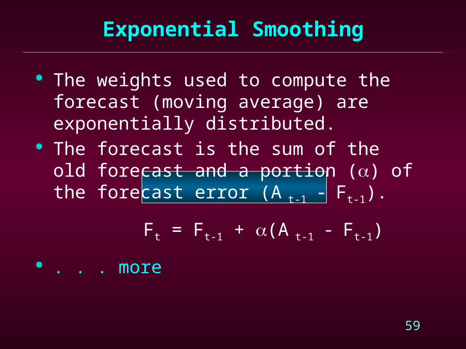
The weights used to compute the forecast (moving average) are exponentially distributed.
The forecast is the sum of the old forecast and a portion (a) of the forecast error (A t-1 - Ft-1).
Ft = Ft-1 + a(A t-1 - Ft-1)
. . . more
Exponential Smoothing
60
Exponential Smoothing
The smoothing constant, a, must be between 0.0 and 1.0.
A large a provides a high impulse response forecast. A small a provides a low impulse response forecast.

61
Example: Central Call Center
Moving AverageCCC wishes to forecast the number of
incoming calls it receives in a day from the customers of one of its clients, BMI. CCC schedules the appropriate number of telephone operators based on projected call volumes.
CCC believes that the most recent 12 days of call volumes (shown on the next slide) are representative of the near future call volumes.

62
Example: Central Call Center
Moving Average Representative Historical Data
Day Calls Day Calls1 159 7 2032 217 8 1953 186 9 1884 161 10 1685 173 11 1986 157 12 159

63
Example: Central Call Center
Moving AverageUse the moving average method with an AP =
3 days to develop a forecast of the call volume in Day 13.
F13 = (168 + 198 + 159)/3 = 175.0 calls

64
Example: Central Call Center
Weighted Moving AverageUse the weighted moving average method with
an AP = 3 days and weights of .1 (for oldest datum), .3, and .6 to develop a forecast of the call volume in Day 13.
F13 = .1(168) + .3(198) + .6(159) = 171.6 calls
Note: The WMA forecast is lower than the MA forecast because Day 13’s relatively low call volume carries almost twice as much weight in the WMA (.60) as it does in the MA (.33).

65
Example: Central Call Center
Exponential SmoothingIf a smoothing constant value of .25 is used
and the exponential smoothing forecast for Day 11 was 180.76 calls, what is the exponential smoothing forecast for Day 13?
F12 = 180.76 + .25(198 – 180.76) = 185.07F13 = 185.07 + .25(159 – 185.07) = 178.55
66
Example: Central Call Center
Forecast Accuracy - MADWhich forecasting method (the AP = 3 moving
average or the a = .25 exponential smoothing) is preferred, based on the MAD over the most recent 9 days? (Assume that the exponential smoothing forecast for Day 3 is the same as the actual call volume.)

67
Example: Central Call Center
AP = 3 a = .25
Day Calls Forec.|Error|Forec.|Error|4 161 187.3 26.3 186.0 25.05 173 188.0 15.0 179.8 6.86 157 173.3 16.3 178.1 21.17 203 163.7 39.3 172.8 30.28 195 177.7 17.3 180.4 14.69 188 185.0 3.0 184.0 4.010 168 195.3 27.3 185.0 17.011 198 183.7 14.3 180.8 17.212 159 184.7 25.7 185.1 26.1
MAD 20.5 18.0

68
Criteria for Selectinga Forecasting Method
Cost Accuracy Data available Time span Nature of products and services Impulse response and noise dampening
69
Criteria for Selectinga Forecasting Method
Cost and Accuracy There is a trade-off between cost and accuracy;
generally, more forecast accuracy can be obtained at a cost.
High-accuracy approaches have disadvantages: Use more data Data are ordinarily more difficult to obtain The models are more costly to design,
implement, and operate Take longer to use

70
Criteria for Selectinga Forecasting Method
Cost and Accuracy Low/Moderate-Cost Approaches – statistical
models, historical analogies, executive-committee consensus
High-Cost Approaches – complex econometric models, Delphi, and market research
71
Criteria for Selectinga Forecasting Method
Data Available Is the necessary data available or can it be
economically obtained? If the need is to forecast sales of a new product,
then a customer survey may not be practical; instead, historical analogy or market research may have to be used.

72
Criteria for Selectinga Forecasting Method
Time Span What operations resource is being forecast and for
what purpose? Short-term staffing needs might best be forecast
with moving average or exponential smoothing models.
Long-term factory capacity needs might best be predicted with regression or executive-committee consensus methods.

73
Criteria for Selectinga Forecasting Method
Nature of Products and Services Is the product/service high cost or high volume? Where is the product/service in its life cycle? Does the product/service have seasonal demand
fluctuations?

74
Criteria for Selectinga Forecasting Method
Impulse Response and Noise Dampening An appropriate balance must be achieved between:
How responsive we want the forecasting model to be to changes in the actual demand data
Our desire to suppress undesirable chance variation or noise in the demand data

75
Reasons for Ineffective Forecasting
Not involving a broad cross section of people Not recognizing that forecasting is integral to
business planning Not recognizing that forecasts will always be wrong Not forecasting the right things Not selecting an appropriate forecasting method Not tracking the accuracy of the forecasting models
76
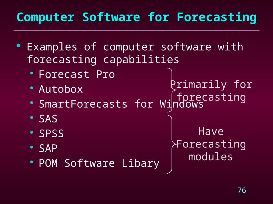
Computer Software for Forecasting
Examples of computer software with forecasting capabilities Forecast Pro Autobox SmartForecasts for Windows SAS SPSS SAP POM Software Libary
Primarily forforecasting
HaveForecasting
modules