Embed Size (px)
Citation preview

Chapter 3
Continuous Random Variables
3.1 Introduction
Rather than summing probabilities related to discrete random variables, here forcontinuous random variables, the density curve is integrated to determine probability.
Exercise 3.1 (Introduction)Patient’s number of visits, X, and duration of visit, Y .
0 1 2 3
0.25
0.75
1
4
probability =
value of function,
F(3) = P(Y < 3) = 5/12
x 0 1 2
0.25
0.50
0.75
1
0 1 2
0.25
0.50
0.75
1
density, pmf f(x)
probability (distribution): cdf F(x)
probability less than 1.5 =
sum of probability
at specific values
P(X < 1.5) = P(X = 0) + P(X = 1)
= 0.25 + 0.50 = 0.75
P(X = 2) = 0.25
0 1 2 3
1/3
1/2
2/3
1
4
density, pdf f(y) = y/6, 2 < y < 4
probability less than 3
= area under curve,
P(Y < 3) = 5/12
x
probability at 3,
P(Y = 3) = 0
probability less than 1.5 =
value of function
F(1.5 ) = P(X < 1.5) = 0.75
_
Figure 3.1: Comparing discrete and continuous distributions
73

74 Chapter 3. Continuous Random Variables (LECTURE NOTES 5)
1. Number of visits, X is a (i) discrete (ii) continuous random variable,and duration of visit, Y is a (i) discrete (ii) continuous random variable.
2. Discrete
(a) P (X = 2) = (i) 0 (ii) 0.25 (iii) 0.50 (iv) 0.75
(b) P (X ≤ 1.5) = P (X ≤ 1) = F (1) = 0.25 + 0.50 = 0.75requires (i) summation (ii) integration and is a value of a(i) probability mass function (ii) cumulative distribution functionwhich is a (i) stepwise (ii) smooth increasing function
(c) E(X) = (i)∑xf(x) (ii)
∫xf(x) dx
(d) V ar(X) = (i) E(X2) − µ2 (ii) E(Y 2) − µ2
(e) M(t) = (i) E(etX
)(ii) E
(etY)
(f) Examples of discrete densities (distributions) include (choose one or more)(i) uniform(ii) geometric(iii) hypergeometric(iv) binomial (Bernoulli)(v) Poisson
3. Continuous
(a) P (Y = 3) = (i) 0 (ii) 0.25 (iii) 0.50 (iv) 0.75
(b) P (Y ≤ 3) = F (3) =∫ 3
2x6dx = x2
12
]x=3
x=2= 32
12− 22
12= 5
12
requires (i) summation (ii) integration and is a value of a(i) probability density function (ii) cumulative distribution func-tionwhich is a (i) stepwise (ii) smooth increasing function
(c) E(Y ) = (i)∑yf(y) (ii)
∫yf(y) dy
(d) V ar(Y ) = (i) E(X2) − µ2 (ii) E(Y 2) − µ2
(e) M(t) = (i) E(etX
)(ii) E
(etY)
(f) Examples of continuous densities (distributions) include (choose one ormore)(i) uniform(ii) exponential(iii) normal (Gaussian)(iv) Gamma(v) chi-square(vi) student-t(vii) F

Section 2. Definitions (LECTURE NOTES 5) 75
3.2 Definitions
Random variable X is continuous if probability density function (pdf) f is continuousat all but a finite number of points and possesses the following properties:
• f(x) ≥ 0, for all x,
•∫∞−∞ f(x) dx = 1,
• P (a < X ≤ b) =∫ baf(x) dx
The (cumulative) distribution function (cdf) for random variable X is
F (x) = P (X ≤ x) =
∫ x
−∞f(t) dt,
and has properties
• limx→−∞ F (x) = 0,
• limx→∞ F (x) = 1,
• if x1 < x2, then F (x1) ≤ F (x2); that is, F is nondecreasing,
• P (a ≤ X ≤ b) = P (X ≤ b)− P (X ≤ a) = F (b)− F (a) =∫ baf(x) dx,
• F ′(x) = ddx
∫ x−∞ f(t) dt = f(x).
xa
cdf F(a) = P(X < a)
density, f(x)
a b
f(x) is positive
P(a < X < b) = F(b) - F(a)total area = 1
_
probability_
probability
Figure 3.2: Continuous distribution
The expected value or mean of random variable X is given by
µ = E(X) =
∫ ∞−∞
xf(x) dx,
the variance is
σ2 = V ar(X) = E[(X − µ)2] = E(X2)− [E(X)]2 = E(X2)− µ2

76 Chapter 3. Continuous Random Variables (LECTURE NOTES 5)
with associated standard deviation, σ =√σ2.
The moment-generating function is
M(t) = E[etX]
=
∫ ∞−∞
etXf(x) dx
for values of t for which this integral exists.Expected value, assuming it exists, of a function u of X is
E[u(X)] =
∫ ∞−∞
u(x)f(x) dx
The (100p)th percentile is a value of X denoted πp where
p =
∫ πp
−∞f(x) dx = F (πp)
and where πp is also called the quantile of order p. The 25th, 50th, 75th percentilesare also called first, second, third quartiles, denoted p1 = π0.25, p2 = π0.50, p3 = π0.75
where also 50th percentile is called the median and denoted m = p2. The mode is thevalue x where f is maximum.
Exercise 4.2 (Definitions)
1. Waiting time.Let the time waiting in line, in minutes, be described by the random variableX which has the following pdf,
f(x) =
{16x, 2 < x ≤ 4,
0, otherwise.
0 1 2 3
1/3
1/2
2/3
1
4 0 1 2 3
0.25
0.75
1
4
probability, cdf F(x)density, pdf f(x)
probability less than 3
= area under curve,
P(X < 3) = 5/12
probability =
value of function,
F(3) = P(X < 3) = 5/12
x x
probability at 3,
P(X = 3) = 0
Figure 3.3: f(x) and F(x)

Section 2. Definitions (LECTURE NOTES 5) 77
(a) Verify function f(x) satisfies the second property of pdfs,∫ ∞−∞
f(x) dx =
∫ 4
2
1
6x dx =
x2
12
]x=4
x=2
=42
12− 22
12=
12
12=
(i) 0 (ii) 0.15 (iii) 0.5 (iv) 1
(b) P (2 < X ≤ 3) = ∫ 3
2
1
6x dx =
x2
12
]x=3
x=2
=32
12− 22
12=
(i) 0 (ii) 512
(iii) 912
(iv) 1
(c) P (X = 3) = P (3− < X ≤ 3) = 32
12− 32
12= 0 6= f(3) = 1
6· 3 = 0.5
(i) True (ii) FalseSo the pdf f(x) = 1
6x determined at some value of x does not determine probability.
(d) P (2 < X ≤ 3) = P (2 < X < 3) = P (2 ≤ X ≤ 3) = P (2 ≤ X < 3)(i) True (ii) Falsebecause P (X = 3) = 0 and P (X = 2) = 0
(e) P (0 < X ≤ 3) = ∫ 3
2
1
6x dx =
x2
12
]x=3
x=2
=32
12− 22
12=
(i) 0 (ii) 512
(iii) 912
(iv) 1Why integrate from 2 to 3 and not 0 to 3?
(f) P (X ≤ 3) = ∫ 3
2
1
6x dx =
x2
12
]x=3
x=2
=32
12− 22
12=
(i) 0 (ii) 512
(iii) 912
(iv) 1
(g) Determine cdf (not pdf) F (3).
F (3) = P (X ≤ 3) =
∫ 3
2
1
6x dx =
x2
12
]x=3
x=2
=32
12− 22
12=
(i) 0 (ii) 512
(iii) 912
(iv) 1
(h) Determine F (3)− F (2).
F (3)−F (2) = P (X ≤ 3)−P (X ≤ 2) = P (2 ≤ X ≤ 3) =
∫ 3
2
1
6x dx =
x2
12
]x=3
x=2
=32
12−22
12=
(i) 0 (ii) 512
(iii) 912
(iv) 1because everything left of (below) 3 subtract everything left of 2 equals what is between 2 and 3

78 Chapter 3. Continuous Random Variables (LECTURE NOTES 5)
(i) The general distribution function (cdf) is
F (x) =
∫ x−∞ 0 dt = 0, x ≤ 2,∫ x2
t6dt = t2
12
]t=xt=2
= x2
12− 4
12, 2 < x ≤ 4,
1, x > 4.
In other words, F (x) = x2
12− 4
12= x2−4
12on (2, 4]. Both pdf density and cdf
distribution are given in the figure above.(i) True (ii) False
(j) F (2) = 22
12− 4
12= (i) 0 (ii) 5
12(iii) 9
12(iv) 1.
(k) F (3) = 32
12− 4
12= (i) 0 (ii) 5
12(iii) 9
12(iv) 1.
(l) P (2.5 < X < 3.5) = F (3.5)− F (2.5) =(
3.52
12− 4
12
)−(
2.52
12− 4
12
)=
(i) 0 (ii) 0.25 (iii) 0.50 (iv) 1.
(m) P (X > 3.5) = 1− P (X ≤ 3.5) = 1− F (3.5) = 1−(
3.52
12− 4
12
)=
(i) 0.3125 (ii) 0.4425 (iii) 0.7650 (iv) 1.
(n) Expected value. The average wait time is
µ = E(X) =
∫ ∞−∞
xf(x) dx =
∫ 4
2
x
(1
6x
)dx =
∫ 4
2
x2
6dx =
x3
18
]4
2
=43
18−23
18=
(i) 239
(ii) 289
(iii) 319
(iv) 359
.
library(MASS) # INSTALL once, RUN once (per session) library MASS
mean <- 4^3/18 - 2^3/18; mean; fractions(mean) # turn decimal to fraction
[1] 3.111111
[1] 28/9
(o) Expected value of function u = x2.
E(X2)
=
∫ ∞−∞
x2f(x) dx =
∫ 4
2
x2
(1
6x
)dx =
∫ 4
2
x3
6dx =
x4
24
]4
2
=44
24−24
24=
(i) 9 (ii) 10 (iii) 11 (iv) 12.
(p) Variance, method 1. Variance in wait time is
σ2 = V ar(X) = E(X2)− µ2 = 10−
(28
9
)2
=
(i) 2381
(ii) 2681
(iii) 3181
(iv) 3581
.
library(MASS) # INSTALL once, RUN once (per session) library MASS
sigma2 <- 10 - (28/9)^2 ; fractions(sigma2) # turn decimal to fraction

Section 2. Definitions (LECTURE NOTES 5) 79
[1] 26/81
(q) Variance, method 2. Variance in wait time is
σ2 = V ar(X) = E[(X − µ)2] =
∫ ∞−∞
(x− µ)2f(x) dx
=
∫ 4
2
(x− 28
9
)2(1
6x
)dx
=
∫ 4
2
(x3
6− 56x2
54+
784x
486
)dx
=x4
24− 56x3
162+
784x2
972
]4
2
=
(i) 2381
(ii) 2681
(iii) 3181
(iv) 3581
.
library(MASS) # INSTALL once, RUN once (per session) library MASS
sigma2 <- (4^4/24 - 56*4^3/162 + 784*4^2/972) - (2^4/24 - 56*2^3/162 + 784*2^2/972)
fractions(sigma2) # turn decimal to fraction
[1] 26/81
(r) Standard deviation. Standard deviation in time spent on the call is,
σ =√σ2 =
√26
81≈
(i) 0.57 (ii) 0.61 (iii) 0.67 (iv) 0.73.
(s) Moment generating function.
M(t) = E[etX ] =
∫ ∞−∞
etxf(x) dx
=
∫ 4
2
etx(
1
6x
)dx
=1
6
∫ 4
2
xetx dx
=1
6etx(x
t− 1
t2
)]4
x=2
=1
6e4t
(4
t− 1
t2
)− 1
6e2t
(2
t− 1
t2
), t 6= 0.
(i) True (ii) Falseuse integration by parts for t 6= 0 case:
∫u dv = uv −
∫v du where u = x, dv = etxdx.

80 Chapter 3. Continuous Random Variables (LECTURE NOTES 5)
(t) Median. Since the distribution function F (x) = x2−412
, then median m =π0.50 occurs when
F (m) = P (X ≤ m) =m2 − 4
12=
1
2
so
m = π0.50 =
√12
2+ 4 ≈
(i) 1.16 (ii) 2.16 (iii) 3.16negative answer m ≈ −3.16 is not in 2 < x ≤ 4, so m 6= −3.16
2. Density with unknown a. Find a such that
f(x) =
{ax2, 1 < x ≤ 5,0, otherwise.
0 1 2 3
0.25
0.50
0.75
1
4 5 0 1 2 3
0.25
0.50
0.75
1
4 5
probability, cdf F(x) = P(X < x)density, pdf f(x)
x x
Figure 3.4: f(x) and F(x)
(a) Find constant a. Since the cdf F (5) = 1, and
F (x) =
∫ x
1
at2 dt = at3
3
]t=xt=1
=ax3
3− a
3=
a(x3 − 1)
3
then
F (5) =a(53 − 1)
3=
124a
3= 1,
so a = (i) 3124
(ii) 2124
(iii) 1124
(b) Determine pdf.f(x) = ax2 =
(i) 3124x2 (ii) 2
124x2 (iii) 1
124x2
Section 2. Definitions (LECTURE NOTES 5) 81
(c) Determine cdf.
F (x) =a(x3 − 1)
3=
3
124× x3 − 1
3=
(i) 3124
(x3 − 1) (ii) 2124
(x3 − 1) (iii) 1124
(x3 − 1)
(d) Determine P (X ≥ 2).
P (X ≥ 2) = 1− P (X < 2) = 1− F (2) = 1− 1
124(23 − 1) =
(i) 61124
(ii) 117124
(iii) 61117
(e) Determine P (X ≥ 4).
P (X ≥ 4) = 1− P (X < 4) = 1− F (4) = 1− 1
124(43 − 1) =
(i) 61124
(ii) 117124
(iii) 61117
(f) Determine P (X ≥ 4|X ≥ 2).
P (X ≥ 4|X ≥ 2) =P (X ≥ 4 ∩X ≥ 2)
P (X ≥ 2)=P (X ≥ 4)
P (X ≥ 2)=
61/124
117/124=
(i) 116124
(ii) 117124
(iii) 61117
(g) Expected value.
µ = E(X) =
∫ ∞−∞
xf(x) dx =
∫ 5
1
x
(3
124x2
)dx =
∫ 5
1
3x3
124dx =
3x4
496
]5
1
=3 · 54
496−3 · 14
496=
(i) 11431
(ii) 11531
(iii) 11631
(iv) 11731
.
(h) Expected value of function u = x2.
E(X2) =
∫ ∞−∞
x2f(x) dx =
∫ 5
1
x2
(3
124x2
)dx =
∫ 5
1
3x4
124dx =
3x5
620
]5
1
=3 · 55
620−3 · 15
620≈
(i) 15.12 (ii) 16.12 (iii) 17.12 (iv) 18.12.
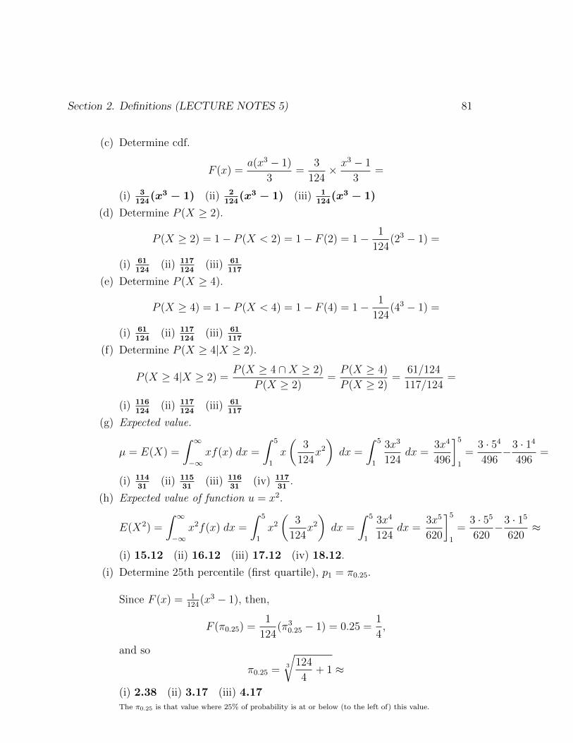
(i) Determine 25th percentile (first quartile), p1 = π0.25.
Since F (x) = 1124
(x3 − 1), then,
F (π0.25) =1
124(π3
0.25 − 1) = 0.25 =1
4,
and so
π0.25 =3
√124
4+ 1 ≈
(i) 2.38 (ii) 3.17 (iii) 4.17The π0.25 is that value where 25% of probability is at or below (to the left of) this value.

82 Chapter 3. Continuous Random Variables (LECTURE NOTES 5)
(j) Determine π0.01.
F (π0.01) =1
124(π3
0.01 − 1) = 0.01,
and soπ0.01 = 3
√0.01 · 124 + 1 ≈
(i) 1.31 (ii) 3.17 (iii) 4.17The π0.01 is that value where 1% of probability is at or below (to the left of) this value.
3. Piecewise pdf. Let random variable X have pdf
f(x) =
x, 0 < x ≤ 1,2− x, 1 < x ≤ 2,0, elsewhere.
0 1 2
0.25
0.50
0.75
1
0 1 2 3
0.25
0.50
0.75
1
probability, cdf F(x) = P(X < x)density, pdf f(x)
x x
Figure 3.5: f(x) and F(x)
(a) Expected value.
µ = E(X) =
∫ ∞−∞
xf(x) dx
=
∫ 1
0
x (x) dx+
∫ 2
1
x (2− x) dx
=
∫ 1
0
x2 dx+
∫ 2
1
(2x− x2
)dx
=
[x3
3
]1
0
+
[2x2
2− x3
3
]2
1
=
(13
3− 03
3
)+
(22 − 23
3
)−(
12 − 13
3
)=
(i) 1 (ii) 2 (iii) 3 (iv) 4.

Section 2. Definitions (LECTURE NOTES 5) 83
(b) E (X2).
E(X2)
=
∫ 1
0
x2 (x) dx+
∫ 2
1
x2 (2− x) dx
=
∫ 1
0
x3 dx+
∫ 2
1
(2x2 − x3
)dx
=
[x4
4
]1
0
+
[2x3
3− x4
4
]2
1
=
(14
4− 04
4
)+
(2(2)3
3− 24
4
)−(
2(1)3
3− 14
4
)=
(i) 46
(ii) 56
(iii) 66
(iv) 76.
(c) Variance.
σ2 = Var(X) = E(X2)− µ2 =
7
6− 12 =
(i) 13
(ii) 14
(iii) 15
(iv) 16.
(d) Standard deviation.
σ =√σ2 =
√1
6≈
(i) 0.27 (ii) 0.31 (iii) 0.41 (iv) 0.53.
(e) Median. Since the distribution function is
F (x) =
0 x ≤ 0∫ x
0t dt = t2
2
]xt=0
= x2
2, 0 < x ≤ 1,∫ x
1(2− t) dt+ F (1) = 2t− t2
2
]xt=1
+ 12
= 2x− x2
2− (2(1)− 12
2) + 1
2, 1 < x ≤ 2,
1, x > 2.
F (1) = 12
, so add 12
to F (x) for 1 < x ≤ 2
then median m occurs when
F (x) =
m2
2= 1
2, 0 < x ≤ 1,
2m− m2
2− 1 = 1
2, 1 < x ≤ 2,
1, x > 2.
so for both 0 < x ≤ 1 and 1 < x ≤ 2, m = (i) 1 (ii) 1.5 (iii) 2
84 Chapter 3. Continuous Random Variables (LECTURE NOTES 5)
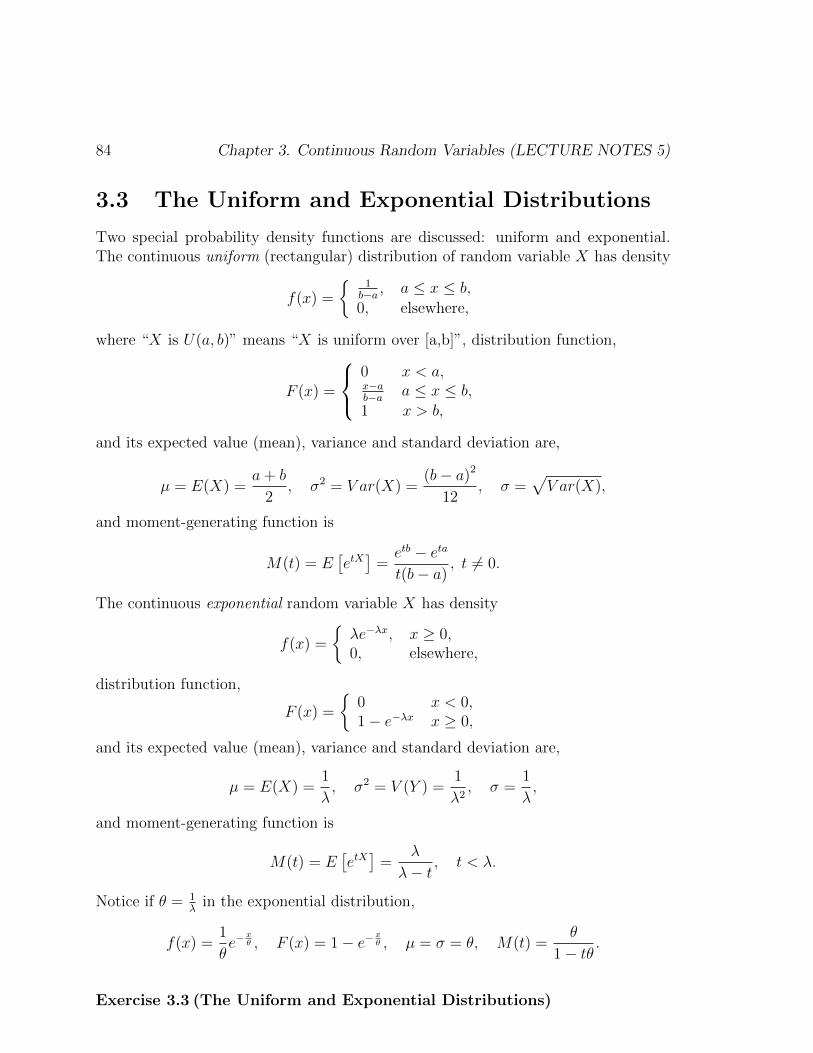
3.3 The Uniform and Exponential Distributions
Two special probability density functions are discussed: uniform and exponential.The continuous uniform (rectangular) distribution of random variable X has density
f(x) =
{1b−a , a ≤ x ≤ b,
0, elsewhere,
where “X is U(a, b)” means “X is uniform over [a,b]”, distribution function,
F (x) =
0 x < a,x−ab−a a ≤ x ≤ b,
1 x > b,
and its expected value (mean), variance and standard deviation are,
µ = E(X) =a+ b
2, σ2 = V ar(X) =
(b− a)2
12, σ =
√V ar(X),
and moment-generating function is
M(t) = E[etX]
=etb − eta
t(b− a), t 6= 0.
The continuous exponential random variable X has density
f(x) =
{λe−λx, x ≥ 0,0, elsewhere,
distribution function,
F (x) =
{0 x < 0,1− e−λx x ≥ 0,
and its expected value (mean), variance and standard deviation are,
µ = E(X) =1
λ, σ2 = V (Y ) =
1
λ2, σ =
1
λ,
and moment-generating function is
M(t) = E[etX]
=λ
λ− t, t < λ.
Notice if θ = 1λ
in the exponential distribution,
f(x) =1
θe−
xθ , F (x) = 1− e−
xθ , µ = σ = θ, M(t) =
θ
1− tθ.
Exercise 3.3 (The Uniform and Exponential Distributions)

Section 3. The Uniform and Exponential Distributions (LECTURE NOTES 5) 85
1. Uniform: potato weights. An automated process fills one bag after anotherwith Idaho potatoes. Although each filled bag should weigh 50 pounds, in fact,because of the differing shapes and weights of each potato, each bag weight, X,is anywhere from 49 pounds to 51 pounds, with uniform density:
f(x) =
{0.5, 49 ≤ x ≤ 51,0, elsewhere.
(a) Since a = 49 and b = 51, the distribution is
F (x) =
0 x < 49,x−4951−49
49 ≤ x ≤ 51,
1 x > 52,
and so graphs of density and distribution are given in the figure.(i) True (ii) False
0 49 50 51 0 49 50 51
0.25
0.50
0.75
1
0.25
0.50
0.75
1
probability, cdf F(x) = P(X < x)density, pdf f(x)
x x
Figure 3.6: Distribution function: continuous uniform
(b) Determine P (49.5 < X < 51) by integrating pdf.
P (49.5 < X < 51) =
∫ 51
49.5
1
2dx =
x
2
]51
x=49.5=
51
2− 49.5
2=
1.5
2
(i) 0.25 (ii) 0.50 (iii) 0.75 (iv) 1.
(c) Determine P (49.5 < X < 51) using cdf.
P (49.5 < X < 51) = F (51)− F (49.5) =51− 49
51− 49− 49.5− 49
51− 49=
(i) 0.25 (ii) 0.50 (iii) 0.75 (iv) 1.1 - punif(49.5,49,51) # uniform P(49.5 < X < 51) = 1 - P(X < 49.5), 49 < x < 51
[1] 0.75

86 Chapter 3. Continuous Random Variables (LECTURE NOTES 5)
(d) The chance the bags weight more than 49.5
P (X > 49.5) = 1− P (X ≤ 49.5) = 1− F (49.5) = 1− 49.5− 49
51− 49=
(i) 0.25 (ii) 0.50 (iii) 0.75 (iv) 1.1 - punif(49.5,49,51) # uniform P(X > 49.5) = 1 - P(X < 49.5), 49 < x < 51
[1] 0.75
(e) What is the mean weight of a bag of potatoes?
µ = E(X) =a+ b
2=
49 + 51
2=
(i) 49 (ii) 50 (iii) 51 (iv) 52.
(f) What is the standard deviation in the weight of a bag of potatoes?
σ =
√(b− a)2
12=
√(51− 49)2
12≈
(i) 0.44 (ii) 0.51 (iii) 0.55 (iv) 0.58.
(g) Determine probability within 1 standard deviation of mean.
P (µ− σ < X < µ+ σ) ≈ P (50− 0.58 < X < 50 + 0.58)
= P (49.42 < X < 50.58)
=
∫ 50.58
49.42
1
2dx =
x
2
]50.58
x=49.42=
(i) 0.44 (ii) 0.51 (iii) 0.55 (iv) 0.58.
(h) Function of X. If it costs $0.0556 (5.56 cents) per pound of potatoes,then the cost of X pounds of potatoes is Y = 0.0556X. Determine theprobability a bag of potatoes chosen at random costs at least $2.78.
P (Y ≥ 2.78) = P (0.0556X ≥ 2.78) = P (X ≥ 50) =
∫ 51
50
1
2dx =
x
2
]51
x=50=
(i) 0.25 (ii) 0.50 (iii) 0.75 (iv) 1.
2. Exponential: atomic decay. Assume atomic time-to-decay obeys exponentialpdf with (inverse) mean rate of decay λ = 3,
f(x) =
{3e−3x, x > 0,0, otherwise.
Section 3. The Uniform and Exponential Distributions (LECTURE NOTES 5) 87
0 1 2 3 4 5 0 1 2 3 4 5
1
2
3
4
1
2
3
4
probability, cdf F(x) = P(X < x)density, pdf f(x)
x x
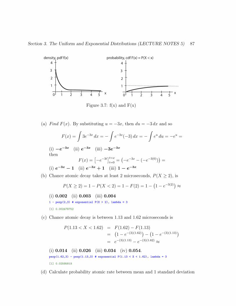
Figure 3.7: f(x) and F(x)
(a) Find F (x). By substituting u = −3x, then du = −3 dx and so
F (x) =
∫3e−3x dx = −
∫e−3x(−3) dx = −
∫eu du = −eu =
(i) −e−3x (ii) e−3x (iii) −3e−3x
thenF (x) =
[−e−3t
]t=xt=0
=(−e−3x − (−e−3(0))
)=
(i) e−3x − 1 (ii) e−3x + 1 (iii) 1 − e−3x
(b) Chance atomic decay takes at least 2 microseconds, P (X ≥ 2), is
P (X ≥ 2) = 1− P (X < 2) = 1− F (2) = 1−(1− e−3(2)
)≈
(i) 0.002 (ii) 0.003 (iii) 0.0041 - pexp(2,3) # exponential P(X > 2), lambda = 3
[1] 0.002478752
(c) Chance atomic decay is between 1.13 and 1.62 microseconds is
P (1.13 < X < 1.62) = F (1.62)− F (1.13)
=(1− e−(3)(1.62)
)−(1− e−(3)(1.13)
)= e−(3)(1.13) − e−(3)(1.62) ≈
(i) 0.014 (ii) 0.026 (iii) 0.034 (iv) 0.054.pexp(1.62,3) - pexp(1.13,3) # exponential P(1.13 < X < 1.62), lambda = 3
[1] 0.02595819
(d) Calculate probability atomic rate between mean and 1 standard deviation

88 Chapter 3. Continuous Random Variables (LECTURE NOTES 5)
below mean. Since λ = 3, so µ = σ = 13, so
P (µ− σ < X < µ) = P
(1
3− 1
3< X <
1
3
)= P
(0 < X <
1
3
)= F
(1
3
)− F (0)
=(
1− e−(3) 13
)−(1− e−(3)(0)
)≈
(i) 0.33 (ii) 0.43 (iii) 0.53 (iv) 0.63.
(e) Check if f(x) is a pdf.∫ ∞0
3e−3x dx = limb→∞
∫ b
0
3e−3x dx = limb→∞
[−e−3x
]x=b
x=0= lim
b→∞
[−e−3b − (−ex(0))
]= 1
or, equivalently,limb→∞
F (b) = limb→∞
1− e−3b = 1
(i) True (ii) False
(f) Show F ′(x) = f(x).
F ′(x) =d
dxF (x) =
d
dx
(1− e−3x
)=
(i) 3e−3x (ii) e−3x + 1 (iii) 1 − e−3x
(g) Determine µ using mgf. Since M(t) = λλ−t ,
M ′(t) =d
dt
(λ
λ− t
)=
λ
(λ− t)2,
so µ = M ′(0) = (i) λ (ii) 1 (iii) 1 − λ (iv) 1λ
.use quotient rule, since f = u
v= λ
λ−t , f′ = vu′−uv′
v2=
(λ−t)(0)−λ(−1)
(λ−t)2 = λ(λ−t)2 = 1
λif t = 0
(h) Memoryless property of exponential. Chance atomic decay lasts at least 10microseconds is
P (X > 10) = 1− F (10) = 1− (1− e−3(10)) =
(i) e−10 (ii) e−20 (iii) e−30 (iv) e−40.
and chance atomic decay lasts at least 15 microseconds, given ithas already lasted at least 5 microseconds is
P (X > 15|X > 5) =P (X > 15, Y > 5)
P (X > 5)=P (X > 15)
P (X > 5)=
1− (1− e−3(15))
1− (1− e−3(5))=

Section 3. The Uniform and Exponential Distributions (LECTURE NOTES 5) 89
(i) e−10 (ii) e−20 (iii) e−30 (iv) e−40.
so, in other words,
P (X > 15|X > 5) =P (X > 15)
P (X > 5)=P (X > 10 + 5)
P (X > 5)= P (X > 10)
orP (X > 10 + 5) = P (X > 10) · P (X > 5)
This is an example of the “memoryless” property of the exponential, it implies time intervals are
independent of one another. Chance of decay after 15 microsecond, given decay after 5 microseconds,
same as chance of decay after 10 seconds; it is as though first 5 microseconds “forgotten”.
3. Verifying if experimental decay is exponential. In an atomic decay study, letrandom variable X be time-to-decay where x ≥ 0. The relative frequencydistribution table and histogram for a sample of 20 atomic decays (measuredin microseconds) from this study are given below. Does this data follow anexponential distribution?
0.60, 0.07, 0.66, 0.17, 0.06, 0.14, 0.15, 0.19, 0.07, 0.360.85, 0.44, 0.71, 1.02, 0.07, 0.21, 0.16, 0.16, 0.01, 0.88
0
0.05
0.10
0.15
0.20
0.25
0.30
0.35
0.40
rela
tiv
e f
req
ue
ncy
time-to-decay (microseconds), x
1.00.80.60.40 0.2
exponential density curve, pdf, f(x)
relative frequency
histogram approximates
density curve
1.2
Figure 3.8: Histogram of exponential decay times

90 Chapter 3. Continuous Random Variables (LECTURE NOTES 5)
bin frequency relative exponentialfrequency probability
(0,0.2] 11 1120
= 0.55 0.44(0.2,0.4] 2 0.10 0.25(0.4,0.6] 2 0.10 0.14(0.6,0.8] 2 0.10 0.08(0.8,1] 2 0.10 0.04(1,1.2] 1 0.05 0.02
(a) Sample mean time-to-decay.
x̄ =0.60 + 0.07 + · · ·+ 0.88
20=
(i) 0.330 (ii) 0.349 (iii) 0.532 (iv) 0.631.x <- c(0.60,0.07,0.66,0.17,0.06,0.14,0.15,0.19,0.07,0.36,0.85,0.44,0.71,1.02,0.07,0.21,0.16,0.16,0.01,0.88)
mean(x)
[1] 0.349
(b) Approximate λ for exponential. Since approximate mean time-to-decay is
µ ≈ x̄ = 0.349,
then, if time-to-decay is exponential, approximate value of λ parameter,since µ = 1
λ, is
λ =1
µ≈ 1
x̄≈
(i) 2.9 (ii) 3.0 (iii) 3.1 (iv) 3.2
and so possible model of data might be exponential density(i) 2.9e−3x (ii) 3e−2.9x (iii) 2.9e−2.9x (iv) 3e−3x.
(c) Approximate probabilities.
P (0 ≤ X ≤ 0.2) =
∫ 0.2
0
2.9e−2.9x dx ≈
(i) 0.44 (ii) 0.25 (iii) 0.14 (iv) 0.08.remaining probabilities in table calculated in a similar way
pexp(0.2,2.9) - pexp(0,2.9) # exponential P(0 < X < 0.2), lambda approx 2.9
[1] 0.4401016
(d) Since sample relative frequencies do not closely match exponential withλ = 2.9 in table, this distribution (i) is (ii) is not a good fit to the data.

Section 4. The Normal Distribution (LECTURE NOTES 5) 91
3.4 The Normal Distribution
The continuous normal distribution of random variable X, defined on the interval(−∞,∞), has pdf with parameters µ and σ, that is, “X is N(µ, σ2)”,
f(x) =1
σ√
2πe−(1/2)[(x−µ)/σ]2 ,
and cdf
F (x) = P (X ≤ x) =
∫ x
−∞
1
σ√
2πe−(1/2)[(t−µ)/σ]2 dt,
and its expected value (mean), variance and standard deviation are,
E(X) = µ, V ar(X) = σ2, σ =√V ar(X),
and mgf is
M(t) = exp
{µt+
σ2t2
2
}.
A normal random variable, X, may be transformed to a standard normal, Z,
f(z) =1√2πe−z
2/2,
where “Z is N(0, 1)” and
Φ(z) = P (Z ≤ z) =
∫ z
−∞
1√2πe−t
2/2 dt,
where µ = 0, σ = 1 and M(t) = et2/2 using the following equation,
Z =X − µσ
.
The distribution of this density does not have a closed–form expression and so must be solved using numerical
integration methods. We will use both R and the tables to obtain approximate numerical answers.
Exercise 3.4 (The Normal Distribution)
1. Nonstandard normal: IQ scores.It has been found that IQ scores, Y , can be distributed by a normal distribution.Densities of IQ scores for 16 year olds, X1, and 20 year olds, X2, are given by
f(x1) =1
16√
2πe−(1/2)[(y−100)/16]2 ,
f(x2) =1
20√
2πe−(1/2)[(y−120)/20]2 .
A graph of these two densities is given in the figure.

92 Chapter 3. Continuous Random Variables (LECTURE NOTES 5)
f(x)
f(x)
x
20 year old IQs
16 year old IQs
µ = 100 µ = 120
σ = 20
σ = 16
Figure 3.9: Normal distributions: IQ scores
(a) Mean IQ score for 20 year olds isµ = (i) 100 (ii) 120 (iii) 124 (iv) 136.
(b) Average (or mean) IQ scores for 16 year olds isµ = (i) 100 (ii) 120 (iii) 124 (iv) 136.
(c) Standard deviation in IQ scores for 20 year oldsσ = (i) 16 (ii) 20 (iii) 24 (iv) 36.
(d) Standard deviation in IQ scores for 16 year olds isσ = (i) 16 (ii) 20 (iii) 24 (iv) 36.
(e) Normal density for 20 year old IQ scores is(i) broader than normal density for 16 year old IQ scores.(ii) as wide as normal density for 16 year old IQ scores.(iii) narrower than normal density for 16 year old IQ scores.
(f) Normal density for the 20 year old IQ scores is(i) shorter than normal density for 16 year old IQ scores.(ii) as tall as normal density for 16 year old IQ scores.(iii) taller than normal density for 16 year old IQ scores.
(g) Total area (probability) under normal density for 20’s IQ scores is(i) smaller than area under normal density for 16’s IQ scores.(ii) the same as area under normal density for 16’s IQ scores.(iii) larger than area under normal density for 16’s IQ scores.
(h) Number of different normal densities:(i) one (ii) two (iii) three (iv) infinity.
2. Percentages: IQ scores.Densities of IQ scores for 16 year olds, X1, and 20 year olds, X2, are given by
f(x1) =1
16√
2πe−(1/2)[(y−100)/16]2 ,
f(x2) =1
20√
2πe−(1/2)[(y−120)/20]2 .

Section 4. The Normal Distribution (LECTURE NOTES 5) 93
f(x)
x100 84
(a)
N(100,16 )P(X > 84) = ? f(x)
f(x)f(x)
x100 96 120
(b)
(d)
P(96 < X < 120) = ?
x12096
N(120,20 )P(96 < X < 120) = ?
(c)
x120 84
N(120,20 )P(X > 84) = ?
N(100,16 )
2
2
2 2
Figure 3.10: Normal probabilities: IQ scores
(a) For the sixteen year old normal distribution, where µ = 100 and σ = 16,
P (X1 > 84) =
∫ ∞84
1
16√
2πe−(1/2)[(y−100)/16]2 dx1 ≈
(i) 0.4931 (ii) 0.9641 (iii) 0.8413 (iv) 0.3849.1 - pnorm(84,100,16) # normal P(X > 84), mean = 100, SD = 16
[1] 0.8413447
(b) For sixteen year old normal distribution, where µ = 100 and σ = 16,P (96 < X1 < 120) ≈ (i) 0.4931 (ii) 0.9641 (iii) 0.8413 (iv) 0.3849.
pnorm(120,100,16) - pnorm(96,100,16) # normal P(96 < X < 120), mean = 100, SD = 16
[1] 0.4930566
(c) For twenty year old, where µ = 120 and σ = 20,P (X2 > 84) ≈ (i) 0.4931 (ii) 0.9641 (iii) 0.8413 (iv) 0.3849.1 - pnorm(84,120,20) # normal P(X > 84), mean = 120, SD = 20
[1] 0.9640697
(d) For twenty year old, where µ = 120 and σ = 20,P (96 < X2 < 120) ≈ (i) 0.4931 (ii) 0.9641 (iii) 0.8413 (iv) 0.3849.
pnorm(120,120,20) - pnorm(96,120,20) # normal P(96 < X < 120), mean = 120, SD = 20
[1] 0.3849303

94 Chapter 3. Continuous Random Variables (LECTURE NOTES 5)
(e) Empirical Rule (68-95-99.7 rule). If X is N(120, 202), find probabilitywithin 1, 2 and 3 SDs of mean.
P (µ−σ < X < µ+σ) = P (120− 20 < X < 120 + 20) = P (100 < X < 140) ≈
(i) 0.683 (ii) 0.954 (iii) 0.997 (iv) 1.
P (µ− 2σ < X < µ+ 2σ) = P (80 < X < 160) ≈
(i) 0.683 (ii) 0.954 (iii) 0.997 (iv) 1.
P (µ− 3σ < X < µ+ 3σ) = P (60 < X < 180) ≈
(i) 0.683 (ii) 0.954 (iii) 0.997 (iv) 1.Empirical rule is true for all X which are N(µ, σ2).
pnorm(140,120,20) - pnorm(100,120,20); pnorm(160,120,20) - pnorm(80,120,20); pnorm(180,120,20) - pnorm(60,120,20)
[1] 0.6826895 [1] 0.9544997 [1] 0.9973002
3. Standard normal.Normal densities of IQ scores for 16 year olds, X1, and 20 year olds, X2,
f(x1) =1
16√
2πe−(1/2)[(y−100)/16]2 ,
f(x2) =1
20√
2πe−(1/2)[(y−120)/20]2 .
Both densities may be transformed to a standard normal with µ = 0 and σ = 1using the following equation,
Z =Y − µσ
.
(a) Since µ = 100 and σ = 16, a 16 year old who has an IQ of 132 isz = 132−100
16= (i) 0 (ii) 1 (iii) 2 (iv) 3
standard deviations above the mean IQ, µ = 100.
(b) A 16 year old who has an IQ of 84 isz = 84−100
16= (i) −2 (ii) −1 (iii) 0 (iv) 1
standard deviations below the mean IQ, µ = 100.
(c) Since µ = 120 and σ = 20, a 20 year old who has an IQ of 180 isz = 180−120
20= (i) 0 (ii) 1 (iii) 2 (iv) 3
standard deviations above the mean IQ, µ = 120.
(d) A 20 year old who has an IQ of 100 isz = 100−120
20= (i) −3 (ii) −2 (iii) −1 (iv) 0
standard deviations below the mean IQ, µ = 120.

Section 4. The Normal Distribution (LECTURE NOTES 5) 95
60 80 100 120 140 160 180 X, nonstandard
-3 -2 -1 0 1 2 3 Z, standard
52 68 84 100 116 132 148 X, nonstandard
-3 -2 -1 0 1 2 3 Z, standard
16 year olds
mean 100, SD 16
20 year olds
mean 120, SD 20
110
Figure 3.11: Standard normal and (nonstandard) normal
(e) Although both the 20 year old and 16 year old scored the same, 110, onan IQ test, the 16 year old is clearly brighter relative to his/her age groupthan is the 20 year old relative his/her age group because
z1 =110− 100
16= 0.625 > z2 =
110− 120
20= −0.5.
(i) True (ii) False
(f) The probability a 20 year old has an IQ greater than 90 is
P (X2 > 90) = P
(Z2 >
90− 120
20
)= P (Z2 > −1.5) ≈
(i) 0.93 (ii) 0.95 (iii) 0.97 (iv) 0.99.1 - pnorm(90,120,20) # normal P(X > 90), mean = 120, SD = 20
1 - pnorm(-1.5) # standard normal P(Z > -1.5), defaults to mean = 0, SD = 1
[1] 0.9331928
Or, using Table C.1 from the text,
P (Z2 > −1.5) = 1− Φ(−1.5) ≈ 1− 0.0668 ≈
(i) 0.93 (ii) 0.95 (iii) 0.97 (iv) 0.99.Table C.1 can only used on standard normal questions, where Z is N(0, 1).
(g) The probability a 20 year old has an IQ between 125 and 135 is
P (125 < X2 < 135) = P
(125− 120
20< Z2 <
135− 120
20
)= P (0.25 < Z2 < 0.75) =
(i) 0.13 (ii) 0.17 (iii) 0.27 (iv) 0.31.
96 Chapter 3. Continuous Random Variables (LECTURE NOTES 5)
pnorm(135,120,20) - pnorm(125,120,20) # normal P(125 < X < 135), mean = 120, SD = 20
pnorm(0.75) - pnorm(0.25) # standard normal P(0.25 < Z < 0.75)
[1] 0.1746663
Or, using Table C.1 from the text,
P (0.25 < Z2 < 0.75) = Φ(0.75)− Φ(0.25) ≈ 0.7734− 0.5987 ≈
(i) 0.13 (ii) 0.17 (iii) 0.27 (iv) 0.31.
(h) If a normal random variable X with mean µ and standard deviation σcan be transformed to a standard one Z with mean µ = 0 and standarddeviation σ = 1 using
Z =X − µσ
,
then Z can be transformed to X using
X = µ+ σZ.
(i) True (ii) False
(i) A 16 year old who has an IQ which is three (3) standards above the meanIQ has an IQ of x1 = 100 + 3(16) =(i) 116 (ii) 125 (iii) 132 (iv) 148.
(j) A 20 year old who has an IQ which is two (2) standards below the meanIQ has an IQ of x2 = 120− 2(20) =(i) 60 (ii) 80 (iii) 100 (iv) 110.
(k) A 20 year old who has an IQ which is 1.5 standards below the mean IQhas an IQ of x2 = 120− 1.5(20) =(i) 60 (ii) 80 (iii) 90 (iv) 95.
(l) The probability a 20 year old has an IQ greater than one (1) standarddeviation above the mean is
P (Z2 > 1) = P (X2 > 120 + 1(20)) = P (X2 > 140) =
(i) 0.11 (ii) 0.13 (iii) 0.16 (iv) 0.18.1 - pnorm(1) # standard normal P(Z > 1), defaults to mean = 0, SD = 1
1 - pnorm(140,120,20) # normal P(X > 140), mean = 120, SD = 20
[1] 0.1586553
(m) Percentile. Determine 1st percentile, π0.01, when X is N(120, 202).
F (π0.01) =
∫ π0.01
−∞
1
20√
2πe−(1/2)[(y−120)/20]2 = 0.01,
and so π0.01 ≈ (i) 72.47 (ii) 73.47 (iii) 75.47
Section 5. Functions of Continuous Random Variables (LECTURE NOTES 5) 97
qnorm(0.01,120,20) # normal 1st percentile, mean = 120, SD = 20
[1] 73.47304
Or, using Table C.1 “backwards”, F (π0.01) = 0.01 when
Z ≈
(i) −2.33 (ii) −2.34 (iii) −2.35
but since X is N(120, 202), 1st percentile
π0.01 = X = µ+ σZ ≈ 120 + 20(−2.33) =
(i) 73.4 (ii) 74.1 (iii) 75.2The π0.01 is that value where 1% of probability is at or below (to the left of) this value.
3.5 Functions of Continuous Random Variables
Assuming cdf F (x) is strictly increasing (as opposed to just monotonically increasing)on a < x < b, one method to determine the pdf of a function, Y = U(X), ofrandom variable X, requires first determining the cdf of X, F (x), then using F (X)to determine the cdf of Y , F (Y ), and finally differentiating the result,
f(y) = F ′(x) =dF
du.
The second fundamental theorem of calculus is sometimes used in this method,
d
dy
∫ u2(y)
u1(y)
fX(x) dx = fX(u2(y))du2
dy− fX(u1(y))
du1
dy.
Related to this is an algorithm for sampling at random values from a random variableX with a desired distribution by using the uniform distribution:
• determine cdf of X, F (x), desired distribution
• find F−1(y): set F (x) = y, solve for x = F−1(y)
• generate values y1, y2, . . . , yn from Y , assumed to be U(0, 1),
• use x = F−1(y) to simulate observed x1, x2, . . . , xn, from desired distribution.
Exercise 3.5 (Functions of Continuous Random Variables)

98 Chapter 3. Continuous Random Variables (LECTURE NOTES 5)
0 1 2 3
0.25
0.50
0.75
1
4
probability, cdf F(x) = P(X < x) = x - x /4
x 0 1 2 3
0.25
0.50
0.75
1
4
probability, cdf F(y) = P(Y < y) = y/2 - y /16
y = 2x
-2 -1 0 1
0.25
0.50
0.75
1
2 y = 2 - 2x0 1 2 3
0.25
0.50
0.75
1
4
probability, cdf F(y) = P(Y < y) = y - y/4
y = x1/2
probability, cdf F(y) = P(Y < y) = (4 + 4y + y )/16
2
2 1/2
2
Figure 3.12: Distributions of various functions of Y = U(X)
1. Determine pdf of Y = U(X), given pdf of X. Consider density
fX(x) =
{1− x
2, 0 ≤ x ≤ 2
0 elsewhere
(a) Calculate pdf of Y = 2X, version 1.
FX(x) =
∫ x
0
(1− t
2
)dt =
(t− t2
4
)t=xt=0
= x− x2
4,
FY (y) = P (Y ≤ y) = P (2X ≤ y) = P(X ≤ y
2
)= FX
(y2
)=
y
2−(y2
)2
4=
y
2− y2
16,
fY (y) = F ′Y (y) =dF
dy=
(i) 32− 2y
32(ii) 1
2− 2y
32(iii) 1
2− y
32(iv) 1
2− y
8,
where since y = 2x, 0 ≤ x ≤ 2 implies 0 ≤ y2≤ 2, or
(i) −1 ≤ y ≤ 2 (ii) −2 ≤ y ≤ 1 (iii) 0 ≤ y ≤ 3 (iv) 0 ≤ y ≤ 4

Section 5. Functions of Continuous Random Variables (LECTURE NOTES 5) 99
(b) Calculate pdf of Y = 2X, version 2.
FY (y) = P (Y ≤ y) = P (2X ≤ y) = P(X ≤ y
2
)= FX
(y2
)=
∫ y2
0
fX(x) dx
fY (y) =d
dy
∫ y2
0
fX(x) dx = fX
(y2
) d
dy
(y2
)− 0 =
(1− y/2
2
)· 1
2=
(i) 32− 2y
32(ii) 1
2− 2y
32(iii) 1
2− y
32(iv) 1
2− y
8,
Second fundamental theorem of calculus used here, notice cdf of FX(x) is not explicitly calculated.
(c) Calculate pdf for Y = 2− 2X.
FY (y) = P (Y ≤ y) = P (2− 2X ≤ y) = P
(X ≥ 2− y
2
)=
∫ 2
2−y2
fX(x) dx,
fY (y) =d
dy
∫ 2
2−y2
fX(x) dx = 0− fX(
2− y2
)d
dy
(2− y
2
)= −
(1−
2−y2
2
)· −1
2=
(i) 32− 2y
32(ii) 1
2+ 2y
32(iii) 1
2+ y
32(iv) 1
4+ y
8,
where since y = 2− 2x, 0 ≤ x ≤ 2 implies 0 ≤ 2−y2≤ 2, or
(i) −1 ≤ y ≤ 2 (ii) −2 ≤ y ≤ 1 (iii) −1 ≤ y ≤ 1 (iv) −2 ≤ y ≤ 2
(d) Calculate pdf for Y = X2.
FY (y) = P (Y ≤ y) = P(X2 ≤ y
)= P (X ≤ √y) =
∫ √y0
fX(x) dx,
fY (y) =d
dy
∫ √y0
fX(x) dx = fX (√y)
d
dy(√y)− 0 =
(1−√y
2
)· 1
2√y
=
(i) 32− 2y
32(ii) 1
2√y− 1
4(iii) 1√
y− 1
4(iv) 1
2√y
+ 14,
Shorten up number of steps, omitted FX(√y).
where y = x2, 0 ≤ x ≤ 2 implies 0 ≤ √y ≤ 2, or(i) 0 ≤ y ≤ 1 (ii) 0 ≤ y ≤ 2 (iii) 0 ≤ y ≤ 3 (iv) 0 ≤ y ≤ 4Although there are two roots, ±√y, only the positive root fits in the positive interval 0 ≤ y ≤ 2.

100 Chapter 3. Continuous Random Variables (LECTURE NOTES 5)
2. Simulate random sample from desired cdf F (x) using uniform.Simulate a random sample of size 5 from X with desired cdf (not pdf),
F (x) =
{0, x < 3
1−(
3x
)3, x ≥ 3
3
1
6x 9 12
cdf: F(x) = P(X < x)
y
inverse cdf: F (y) = P(Y < y)-1
(a) sample point y
chosen at random from
(assume) uniform U(0,1)
(b) generates sample point x chosen
at random from desired cdf F (y)-1
Figure 3.13: Distribution y = F (x) and inverse x = F−1(y)
(a) Determine cdf of X, desired F (x).
It is given (does not need to be worked out in this case): F (x) = 1−(
3x
)3
(b) Find inverse cdf F−1(y). Since F (x) = 1−(
3x
)3= y, then
x = F−1(y) = (i)(3x
)3(ii) 1−
(9x
)3(iii) 1−3(1−y)−
13 (iv) 3(1−y)−
13
(c) Generate values y1, y2, y3, y4, y5 from Y , assumed to be U(0, 1).One possible random sample of size 5 from uniform on U(0, 1) gives
0.2189, 0.9913, 0.5775, 0.2846, 0.8068.
y <- runif(5); y
[1] 0.2189 0.9913 0.5775 0.2846 0.8068
(d) Use x = F−1(y) to generate observed x1, x2, . . . , xn, from desired F (x).Complete the following table.
y sample from U(0, 1) 0.2189 0.9913 0.5775 0.2846 0.8068
x = F−1(y) = 3(1− y)−13 3.2575 14.586
y <- c(0.2189,0.9913,0.5775,0.2846,0.8068)
x <- 3*(1-y)^{-1/3}; x
[1] 3.257510 14.586402 3.998027 3.354323 5.189421