Chapter 3 Cramer-Rao Lower Bound

Abbreviated: CRLB or sometimes just CRB

CRLB is a lower bound on the variance of any unbiasedestimator:

The CRLB tells us the best we can ever expect to be able to do (w/ an unbiased estimator)

then, ofestimator unbiased an is � If θθ

)()()()( ���2� θθσθθσ

θθθθ CRLBCRLB ≥⇒≥

What is the Cramer-Rao Lower Bound

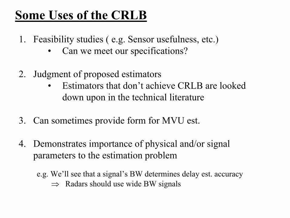
1. Feasibility studies ( e.g. Sensor usefulness, etc.) � Can we meet our specifications?

2. Judgment of proposed estimators� Estimators that don�t achieve CRLB are looked

down upon in the technical literature

3. Can sometimes provide form for MVU est.

4. Demonstrates importance of physical and/or signal parameters to the estimation problem

e.g. We�ll see that a signal�s BW determines delay est. accuracy⇒ Radars should use wide BW signals

Some Uses of the CRLB

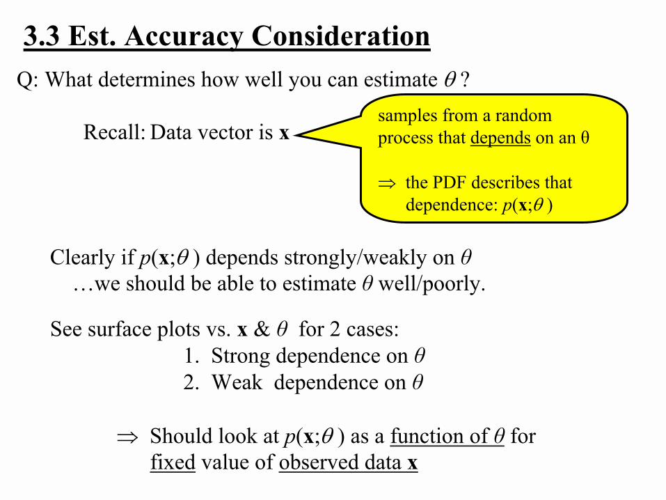
Q: What determines how well you can estimate θ ?

Recall: Data vector is x

3.3 Est. Accuracy Consideration

samples from a random process that depends on an θ

⇒ the PDF describes that dependence: p(x;θ )

Clearly if p(x;θ ) depends strongly/weakly on θ�we should be able to estimate θ well/poorly.

See surface plots vs. x & θ for 2 cases:1. Strong dependence on θ2. Weak dependence on θ

⇒ Should look at p(x;θ ) as a function of θ for fixed value of observed data x

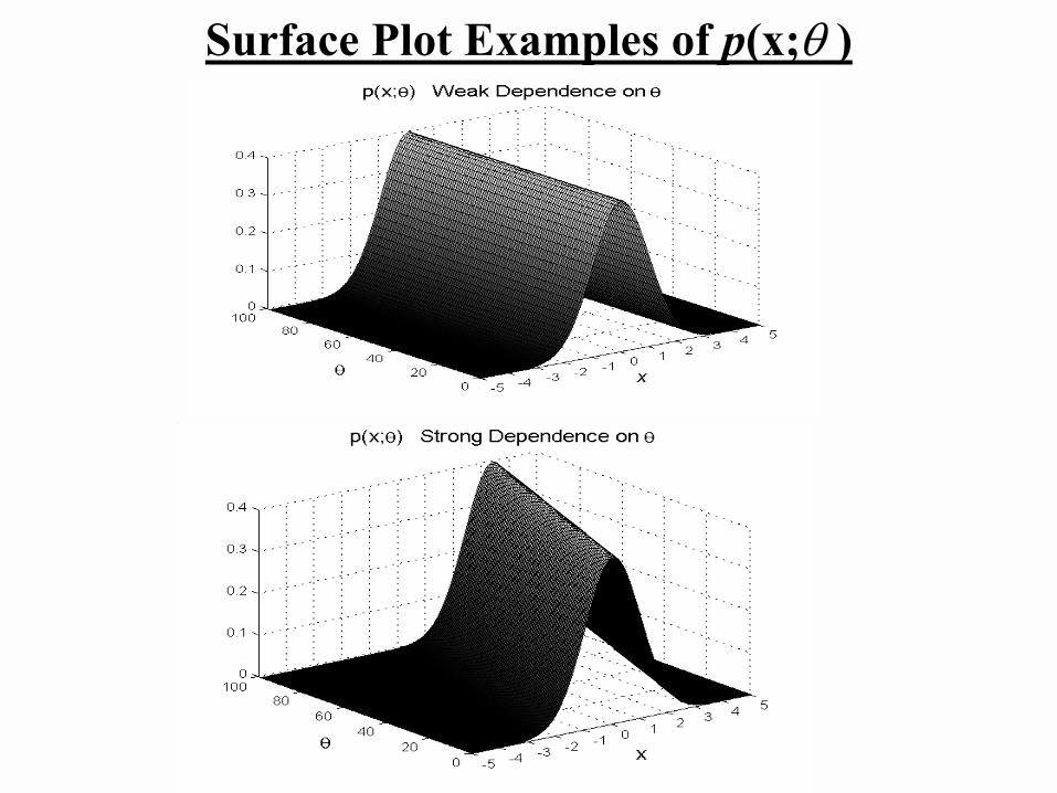
Surface Plot Examples of p(x;θ )

( )

−−= 2

2

2 2)]0[(exp

2

1];0[σπσ

AxAxp

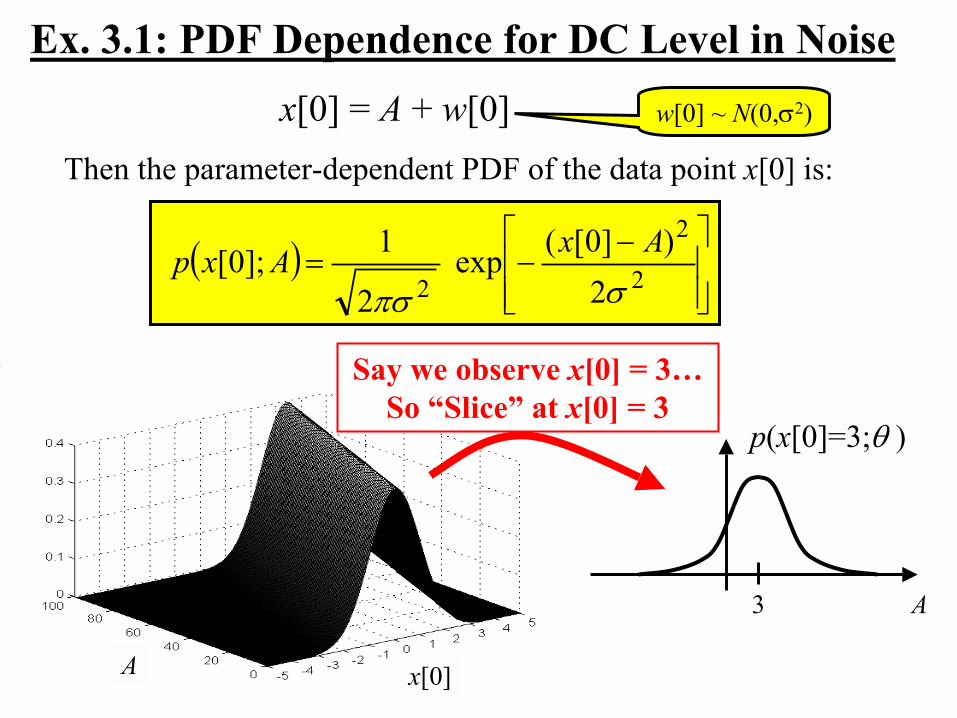
x[0] = A + w[0]

Ex. 3.1: PDF Dependence for DC Level in Noisew[0] ~ N(0,σ2)

Then the parameter-dependent PDF of the data point x[0] is:

A x[0]

A3

p(x[0]=3;θ )

Say we observe x[0] = 3�So �Slice� at x[0] = 3

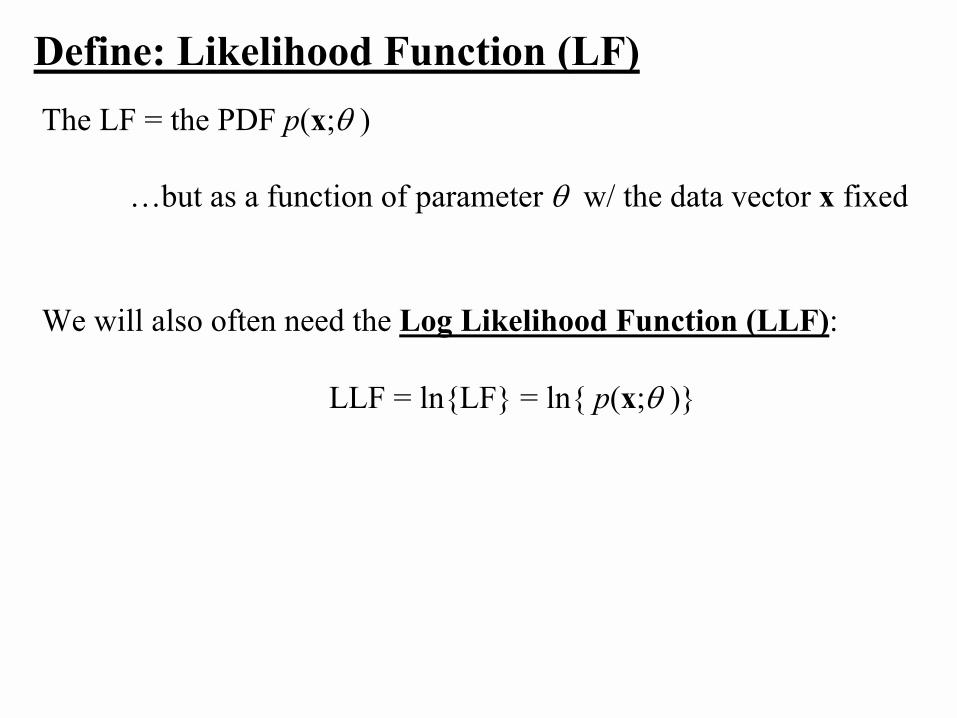
The LF = the PDF p(x;θ )

�but as a function of parameter θ w/ the data vector x fixed

Define: Likelihood Function (LF)

We will also often need the Log Likelihood Function (LLF):

LLF = ln{LF} = ln{ p(x;θ )}

LF Characteristics that Affect Accuracy Intuitively: �sharpness� of the LF sets accuracy� But How???Sharpness is measured using curvature: ( )

valuetruedatagiven 2

2 ;ln

==∂

∂−

θθ

θx

xp

Curvature ↑ ⇒ PDF concentration ↑ ⇒ Accuracy ↑

But this is for a particular set of data� we want �in general�:So�Average over random vector to give the average curvature:

( )

valuetrue2

2 ;ln

=

∂

∂−

θθ

θxpE�Expected sharpness

of LF�

E{�} is w.r.t p(x;θ )

Theorem 3.1 CRLB for Scalar Parameter

Assume �regularity� condition is met: θθθ

∀=

∂∂ 0);(ln xpE

E{�} is w.r.t p(x;θ )

Then( )

valuetrue2

22�

;ln

1

=

∂∂

−

≥

θ

θ

θθ

σxpE

3.4 Cramer-Rao Lower Bound

( ) ( ) dxxpppE );(;ln;ln2

2

2

2θ

θθ

θθ

∫ ∂

∂=

∂

∂ xx

Right-Hand Side is CRLB

1. Write log 1ikelihood function as a function of θ: � ln p(x;θ )

2. Fix x and take 2nd partial of LLF: � ∂2ln p(x;θ )/∂θ 2

3. If result still depends on x:� Fix θ and take expected value w.r.t. x� Otherwise skip this step

4. Result may still depend on θ: � Evaluate at each specific value of θ desired.

5. Negate and form reciprocal

Steps to Find the CRLB

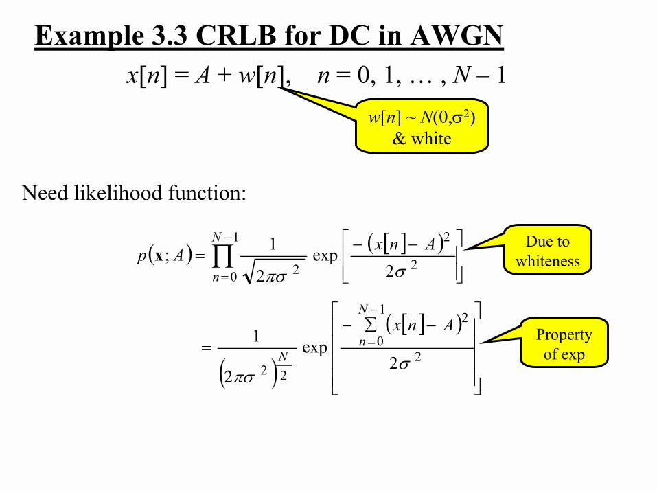
Need likelihood function:

( ) [ ]( )

( )[ ]( )

−∑−

=

−−=

−

=

−

=∏

2

21

0

22

1

02

2

2

2exp

2

1

2exp

2

1;

σπσ

σπσ

Anx

AnxAp

N

nN

N

nx

Example 3.3 CRLB for DC in AWGNx[n] = A + w[n], n = 0, 1, � , N � 1

w[n] ~ N(0,σ2)& white

Due to whiteness

Property of exp

( ) [ ]( )!!! "!!! #$!! "!! #$

?(~~)

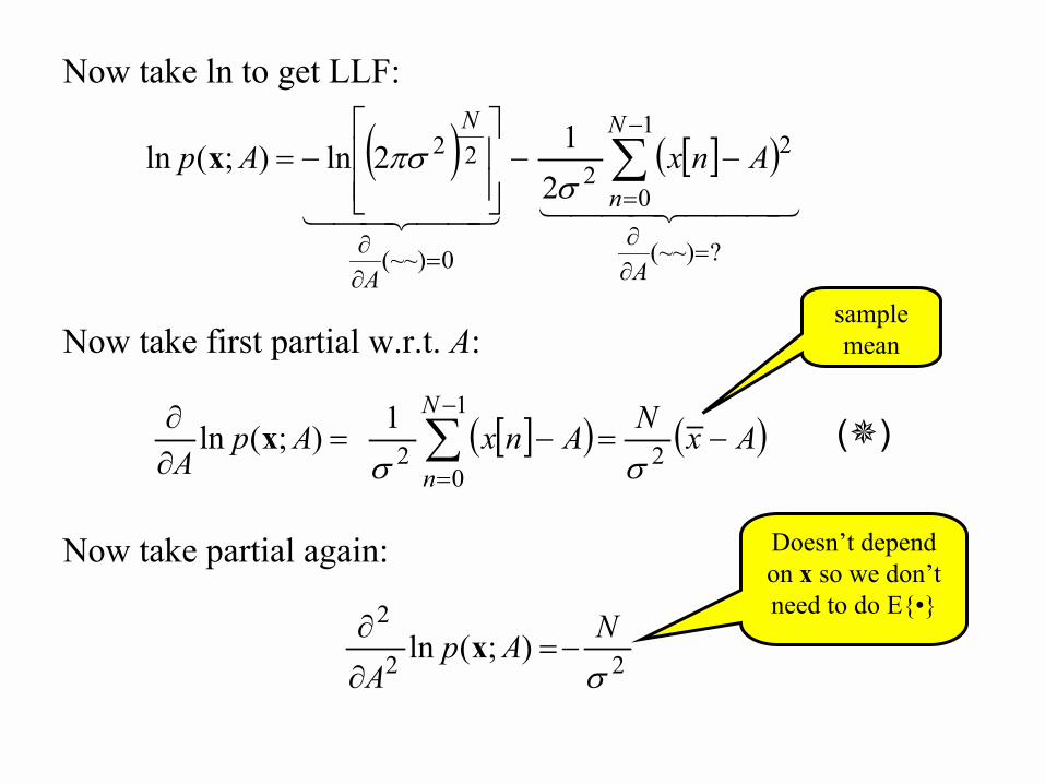
1

0

22

0(~~)

22

212ln);(ln

=∂∂

−

=

=∂∂

∑ −−

−=

A

N

n

A

NAnxAp

σπσx

Now take ln to get LLF:

[ ]( ) ( )AxNAnxApA

N

n−=−=

∂∂ ∑

−

=2

1

02

1);(lnσσ

x

Now take first partial w.r.t. A:sample mean

(!)

Now take partial again:

22

2);(ln

σNAp

A−=

∂

∂ x

Doesn�t depend on x so we don�t need to do E{�}

Since the result doesn�t depend on x or A all we do is negate and form reciprocal to get CRLB:

( ) NpE

CRLB2

valuetrue2

2 ;ln

1 σ

θθ

θ

=

∂∂

−

=

=

xN

A2

}�var{ σ≥

� Doesn�t depend on A� Increases linearly with σ 2

� Decreases inversely with N

CRLB

For fixed N

σ 2

A

CRLB

For fixed N & σ 2

CRLB Doubling DataHalves CRLB!

N

For fixed σ 2

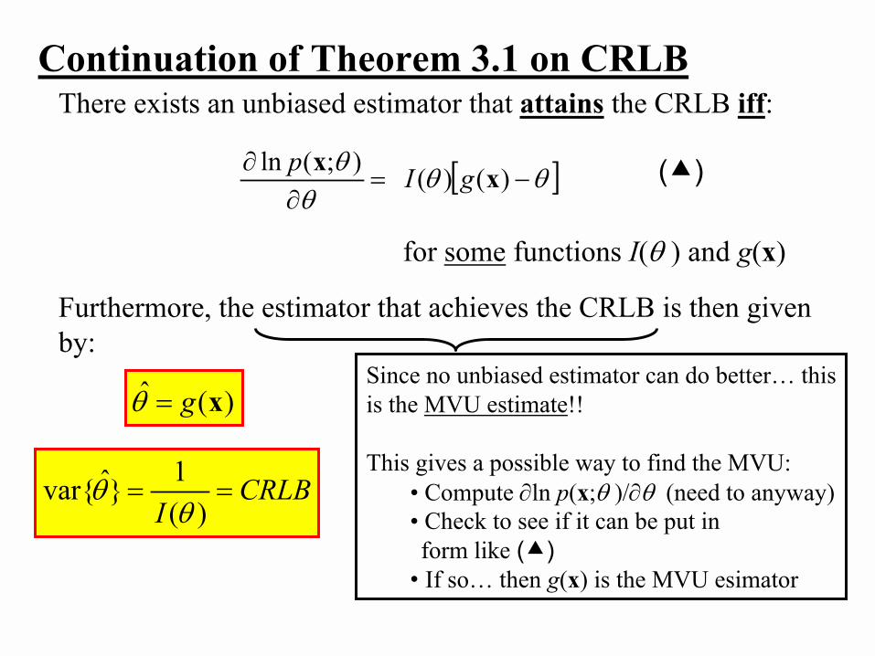
Continuation of Theorem 3.1 on CRLBThere exists an unbiased estimator that attains the CRLB iff:

[ ]θθθ

θ−=

∂∂ )()();(ln xx gIp

for some functions I(θ ) and g(x)

Furthermore, the estimator that achieves the CRLB is then given by:

)(� xg=θ

(!)

Since no unbiased estimator can do better� this is the MVU estimate!!

This gives a possible way to find the MVU:� Compute ∂ln p(x;θ )/∂θ (need to anyway)� Check to see if it can be put in form like (!)

� If so� then g(x) is the MVU esimator

with CRLBI

==)(

1}�var{θ

θ

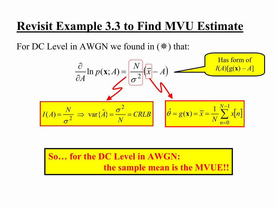
Revisit Example 3.3 to Find MVU Estimate

( )AxNApA

−=∂∂

2);(lnσ

x

For DC Level in AWGN we found in (!) that:Has form of

I(A)[g(x) � A]

[ ]∑−

====

1

0

1)(�N

nnx

Nxg xθCRLB

NANAI ==⇒=

2

2 }�var{)( σσ

So� for the DC Level in AWGN: the sample mean is the MVUE!!

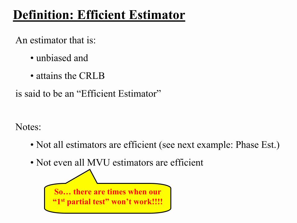
Definition: Efficient Estimator

An estimator that is:

� unbiased and

� attains the CRLB

is said to be an �Efficient Estimator�

Notes:

� Not all estimators are efficient (see next example: Phase Est.)

� Not even all MVU estimators are efficient

So� there are times when our �1st partial test� won�t work!!!!

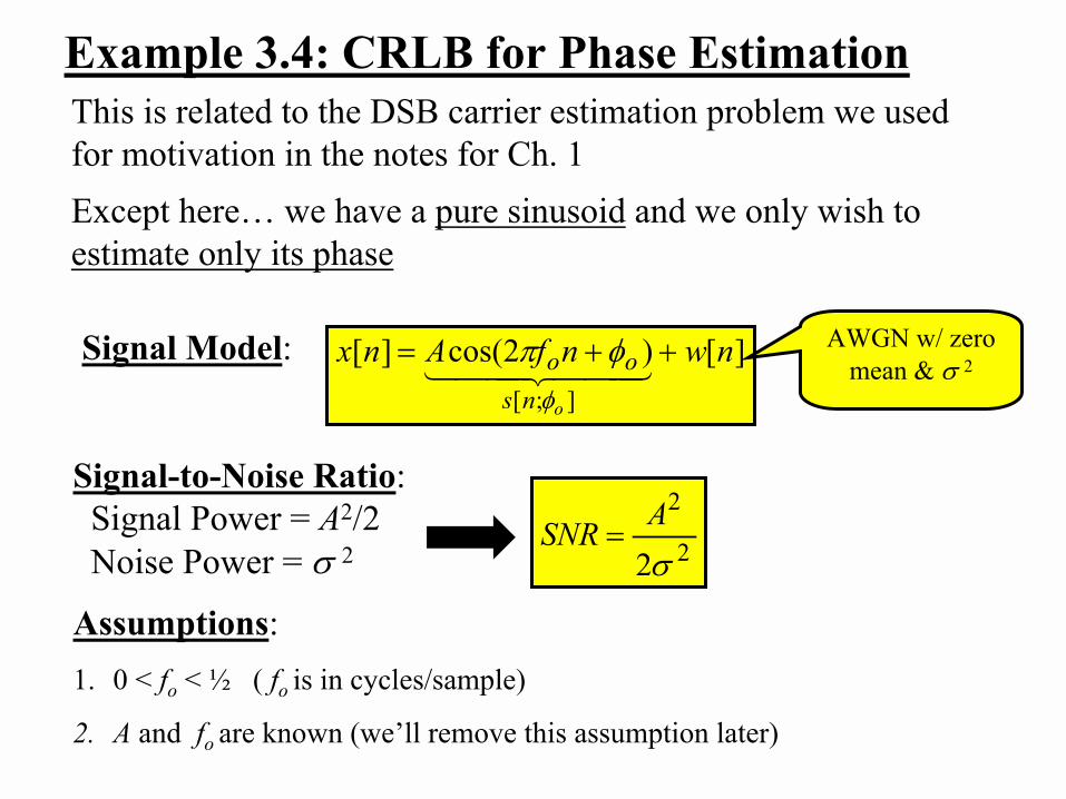
Example 3.4: CRLB for Phase EstimationThis is related to the DSB carrier estimation problem we used for motivation in the notes for Ch. 1Except here� we have a pure sinusoid and we only wish to estimate only its phase

Signal Model: ][)2cos(][];[

nwnfAnxons

oo ++= !!! "!!! #$φ

φπ AWGN w/ zero mean & σ 2

Assumptions:1. 0 < fo < ½ ( fo is in cycles/sample)

2. A and fo are known (we�ll remove this assumption later)

Signal-to-Noise Ratio: Signal Power = A2/2Noise Power = σ 2 2

2

2σASNR =

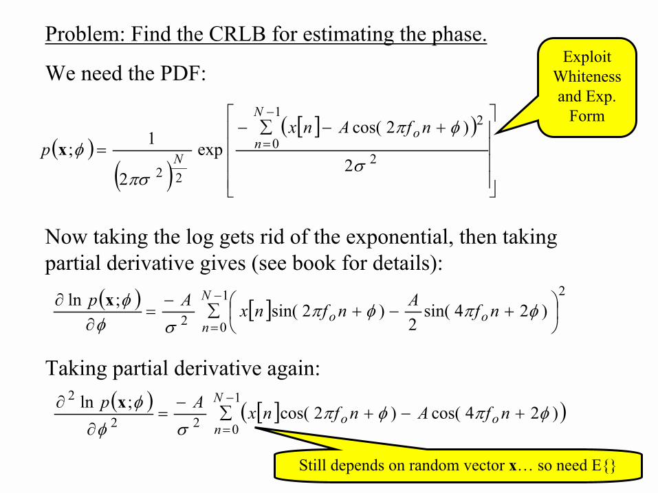
Problem: Find the CRLB for estimating the phase.

We need the PDF:

( )( )

[ ]( )

+−∑−

=

−

=2

21

0

22 2

)2cos(exp

2

1;σ

φπ

πσ

φnfAnx

po

N

nNx

Exploit Whiteness and Exp.

Form

Now taking the log gets rid of the exponential, then taking partial derivative gives (see book for details):

( ) [ ]21

02 )24sin(2

)2sin(;ln

+−+∑

−=

∂∂ −

=φπφπ

σφφ nfAnfnxAp

ooN

n

x

Taking partial derivative again:( ) [ ]( ))24cos()2cos(;ln 1

022

2φπφπ

σφφ

+−+∑−

=∂

∂ −

=nfAnfnxAp

ooN

n

x

Still depends on random vector x� so need E{}

Taking the expected value:

( ) [ ]( )

[ ]{ }( ))24cos()2cos(

)24cos()2cos(;ln

1

02

1

022

2

φπφπσ

φπφπσφ

φ

+−+∑=

+−+∑=

∂

∂−

−

=

−

=

nfAnfnxEA

nfAnfnxAEpE

ooN

n

ooN

n

x

E{x[n]} = A cos(2π fon + φ )

So� plug that in, get a cos2 term, use trig identity, and get

( ) SNRNNAnfApEN

no

N

n×=≈

+−=

∂

∂− ∑∑

−

−

−

=2

21

0

1

02

2

2

2

2)24cos(1

2;ln

σφπ

σφφx

= N << N iffo not near 0 or ½

nN-1

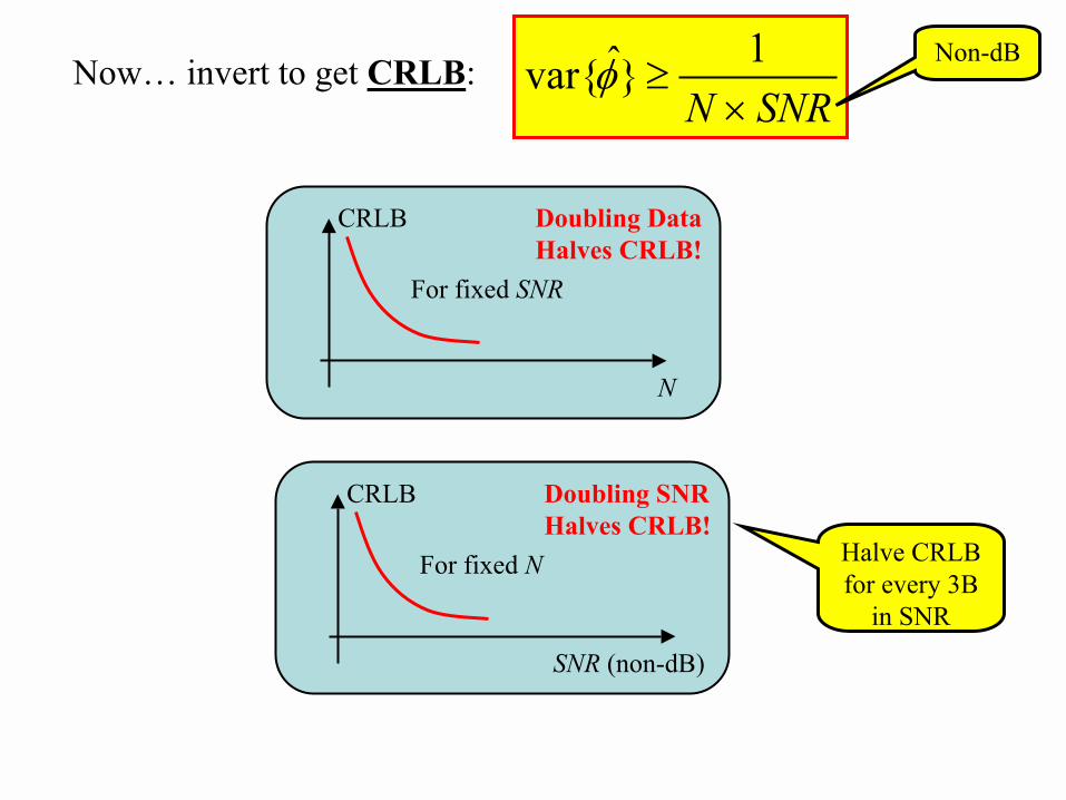
Now� invert to get CRLB:SNRN ×

≥1}�var{φ

CRLB Doubling DataHalves CRLB!

N

For fixed SNR

Non-dB

CRLB Doubling SNRHalves CRLB!

SNR (non-dB)

For fixed N Halve CRLB for every 3B

in SNR

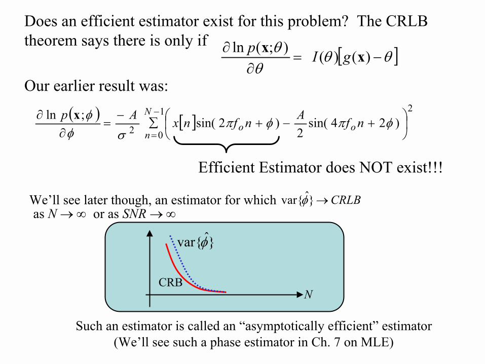
Does an efficient estimator exist for this problem? The CRLB theorem says there is only if

[ ]θθθ

θ−=

∂∂ )()();(ln xx gIp

( ) [ ]21

02 )24sin(2

)2sin(;ln

+−+∑

−=

∂∂ −

=φπφπ

σφφ nfAnfnxAp

ooN

n

x

Our earlier result was:

Efficient Estimator does NOT exist!!!

We�ll see later though, an estimator for which CRLB→}�var{φas N →∞ or as SNR →∞

Such an estimator is called an �asymptotically efficient� estimator(We�ll see such a phase estimator in Ch. 7 on MLE)

CRBN

}�var{φ