91

C H A P T E R 3

FISCAL POLICY

The American Taxpayer Relief Act of 2012 (ATRA), which was enacted on January 2, 2013, permanently extended the 2001 and 2003 Federal

income tax cuts for 98 percent of taxpayers. The tax relief act reflects the approach supported by the President to reduce the Federal budget deficit—an approach that balances responsible reductions in government spending with new revenues and increased progressivity of the tax code. The new law extended the expansions of several tax credits enacted in the American Recovery and Reinvestment Act of 2009 (the Recovery Act) that have pro-vided economic opportunities through tax relief and college expense assis-tance to 25 million low- and middle-income students and working families each year. In addition, the new law prevented a substantial cut in Medicare physician payment rates, extended emergency unemployment insurance benefits to protect 2 million workers from losing their benefits in January 2013, and permanently indexed to inflation the exemption amounts for the Alternative Minimum Tax (AMT) to provide tax certainty to tens of millions of middle-class families. The permanent fix to the AMT will protect middle-class families from being subject to a tax designed to ensure that wealthy taxpayers pay their fair share in taxes.

Together with the additional Medicare and investment income taxes for high-income taxpayers in the Affordable Care Act (ACA), ATRA has made the Federal tax system more progressive. Figure 3-1 shows the trends in average Federal individual income and employment tax rates by income class. These average tax rates, defined as the share of taxpayer income paid in taxes, are measured by holding the distribution of taxpayer income constant over time (using the 2005 distribution with incomes adjusted for growth in the National Average Wage Index) to isolate the effects of tax law changes. The tax law changes in 2013 increased the average tax rate for taxpayers in the top 1 percent and the top 0.1 percent of the income distribution by 4.9 and 6.5 percentage points, respectively, while leaving individual income tax rates unchanged for 98 percent of Americans.

92 | Chapter 3

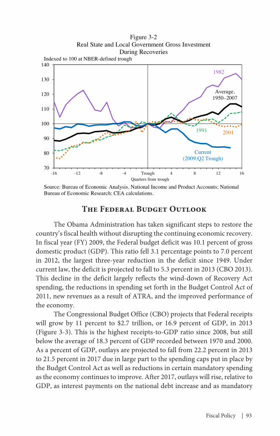
Another recent development in government finance is that the fiscal outlook for State and local governments has improved, although expen-ditures remain below pre-recession levels and State and local investment spending remains notably low. As shown in Figure 3-2, the continued decline in State and local investment is atypical. In other recoveries, State and local governments’ gross real investment was typically flat for several quarters following a business-cycle trough and then increased, but, in this recovery, gross investment has failed to rebound.

This chapter highlights the declining Federal budget deficit since 2009 and the additional work needed to achieve medium- and long-term fiscal health. It then outlines the principles for Federal income tax reform set forth by President Obama in September 2011 and describes specific plans pro-posed by the Administration to meet these goals. The enactment of ATRA is a step toward achieving these goals, but substantial work remains to make the tax code more equitable and efficient. The chapter also reviews the State and local budget outlook and the Federal Government’s role in mitigating the recent recession’s effect on government finances at these levels. Finally, the chapter discusses the long-term financial challenge facing State and local governments from the underfunding of pension plans.

0

10

20

30

40

50

60

1960 1965 1970 1975 1980 1985 1990 1995 2000 2005 2010Note: Average Federal (individual income plus payroll) tax rates for a 2005 sample of taxpayers after adjusting for growth in the National Average Wage Index. Source: Internal Revenue Service, Statistics of Income Public Use File; National Bureau of Economic Research, TAXSIM (preliminary for 2012 and 2013); CEA calculations.

Middle 20 percent

Top 0.1 percent

Top 1 percent

Average tax rate, percent

Figure 3-1Average Tax Rates for Selected Income Groups Under a Fixed Income Distribution, 1960–2013

2013

Fiscal Policy | 93

The Federal Budget Outlook

The Obama Administration has taken significant steps to restore the country’s fiscal health without disrupting the continuing economic recovery. In fiscal year (FY) 2009, the Federal budget deficit was 10.1 percent of gross domestic product (GDP). This ratio fell 3.1 percentage points to 7.0 percent in 2012, the largest three-year reduction in the deficit since 1949. Under current law, the deficit is projected to fall to 5.3 percent in 2013 (CBO 2013). This decline in the deficit largely reflects the wind-down of Recovery Act spending, the reductions in spending set forth in the Budget Control Act of 2011, new revenues as a result of ATRA, and the improved performance of the economy.

The Congressional Budget Office (CBO) projects that Federal receipts will grow by 11 percent to $2.7 trillion, or 16.9 percent of GDP, in 2013 (Figure 3-3). This is the highest receipts-to-GDP ratio since 2008, but still below the average of 18.3 percent of GDP recorded between 1970 and 2000. As a percent of GDP, outlays are projected to fall from 22.2 percent in 2013 to 21.5 percent in 2017 due in large part to the spending caps put in place by the Budget Control Act as well as reductions in certain mandatory spending as the economy continues to improve. After 2017, outlays will rise, relative to GDP, as interest payments on the national debt increase and as mandatory

70

80

90

100

110

120

130

140

-16 -12 -8 -4 Trough 4 8 12 16

Figure 3-2Real State and Local Government Gross Investment

During RecoveriesIndexed to 100 at NBER-defined trough

Quarters from trough

1982

Current (2009:Q2 Trough)

1991 2001

Average,1950–2007

Source: Bureau of Economic Analysis, National Income and Product Accounts; National Bureau of Economic Research; CEA calculations.

94 | Chapter 3

health and retirement spending grows in accordance with the cost of health care and an aging population. Over the long term, these factors—rising health costs and changing demographics—are the primary drivers of fiscal imbalance (CBO 2012).

The Administration’s goal of stabilizing the debt-to-GDP ratio requires reducing the deficit to 3 percent of GDP or lower. Increases in revenues and decreases in outlays in recent years have brought the Federal budget deficit—the gap between outlays and receipts—closer to that target (Figure 3-4). CBO projects that, under current law, deficits will continue to shrink over the next few years, falling below 3 percent of GDP by 2015, but will then increase steadily to 3.8 percent of GDP by 2022. Under current law, publicly held Federal debt is projected to reach 77 percent of GDP in 2023 (Figure 3-5).

Although enacted legislation and overall economic improvements will help reduce the budget deficit, other structural changes will be needed to achieve fiscal sustainability. The President has put forward a balanced deficit-reduction plan to achieve approximately $1.8 trillion in savings through a combination of reductions in discretionary spending, savings in entitlement programs, and new revenue raised by reforming tax expendi-tures and closing tax loopholes. When added to the more than $2.5 trillion in deficit reduction the President already signed into law, the total deficit

10

12

14

16

18

20

22

24

26

28

1970 1975 1980 1985 1990 1995 2000 2005 2010 2015 2020

Average outlays1970–2000

Outlays

Source: OMB (2012b); CBO (2013).

Percent of GDP

Figure 3-3Federal Receipts and Outlays, 1970–2023

2023

ReceiptsAverage receipts

1970–2000

Fiscal year

Actual Projected

Fiscal Policy | 95

1970 1975 1980 1985 1990 1995 2000 2005 2010 2015 2020-4

-2

0

2

4

6

8

10

12

Source: OMB (2012b); CBO (2013).

Percent of GDP

Figure 3-4Federal Budget Deficit, 1970–2023

Fiscal year

2023

Actual Projected

0

10

20

30

40

50

60

70

80

90

1970 1975 1980 1985 1990 1995 2000 2005 2010 2015 2020

Source: OMB (2012b); CBO (2013).

Percent of GDP

Figure 3-5Federal Debt Held by the Public, 1970–2023

2023

Fiscal year

Actual Projected

96 | Chapter 3

reduction would amount to more than $4 trillion over ten years, a goal set by the President to stabilize the debt-to-GDP ratio and to put the country on a sustainable fiscal path over the next decade.

Federal Income Tax Reform

A fair, simple, and efficient tax code lays the foundation for job cre-ation, economic growth, and an equitable society. Recognizing the crucial role tax reform can play in deficit reduction and economic growth, President Obama set forth a list of principles in September 2011 for comprehensive tax reform. These principles include lowering tax rates, cutting inefficient and unfair tax breaks, observing the “Buffett Rule” to enhance tax fairness, reducing the deficit, and increasing job creation and growth in the United States (OMB 2011).

Because revenue must be raised to finance essential services provided by the government, sound tax policy attempts to raise revenue fairly and effi-ciently. A number of notions of fairness can help guide tax policy: “horizon-tal equity” demands equal treatment of equals; the ability-to-pay principle prescribes that a taxpayer’s burden should be related to her ability to pay; the benefit principle suggests that a taxpayer’s burden should be related to the benefits she receives from government services. Such notions of fairness are often incomplete, and sometimes they are in conflict with each other. Still, these principles can serve as useful guides.

Fairness, however, must be balanced with efficiency. High tax rates, combined with a complex tax system and a narrow tax base (that is, with many deductions, exclusions, or exemptions), provide incentives for tax-payers to shift income between the individual and corporate tax bases, re-time income, and alter behavior in other ways to reduce tax liability (Saez, Slemrod, and Giertz 2012). In addition, although tax subsidies could encour-age socially beneficial activity or correct market failures, when there are no externalities or other market failures, tax provisions that favor one activity over another can lead to an inefficient allocation of resources.

A key feature of the tax code is the schedule of statutory tax rates on marginal income. To achieve myriad tax, economic, and social policy goals, the tax code also contains a dizzying web of deductions, exemptions, exclu-sions, credits, and special treatment of certain income. The fact that taxpay-ers modify their behavior to reap the benefits of special tax provisions is bittersweet. On one hand, it means that well-thought-out tax provisions that are designed to encourage a particular activity are working. On the other hand, a taxpayer determined to avoid liability can engage in tax avoidance

Fiscal Policy | 97

and thereby expend socially unproductive resources navigating the jungle of tax provisions.1

Tax ExpendituresThe tax code contains numerous special tax provisions, referred to

as “tax expenditures,” which lead the tax system to deviate from taxing economic income (Box 3-1). Economic income generally follows the Haig-Simons definition of comprehensive income as consumption plus changes in net worth. Relative to a tax structure built on a comprehensive income measure, tax expenditures erode the tax base, causing the government to forgo revenue, but they provide important tax benefits to individuals and families. How such benefits are distributed over the income distribution varies widely across tax provisions. To assess the distributional effects of a given tax expenditure, the Treasury Department estimated the tax benefits of each major individual income tax expenditure under 2013 income tax law for taxpayers in different income classes.

As illustrated in Figure 3-6, the Earned Income Tax Credit (EITC) and the Child Tax Credit (including the refundable portion) provide substantial benefits to taxpayers in the lowest income quintile but have little impact on the after-tax income of taxpayers in the top three income quintiles. By contrast, the bottom two income quintiles receive almost no benefits from tax expenditures like the charitable giving deduction and deductions for State and local taxes. Almost all of those tax benefits accrue to taxpayers in the top two income quintiles. Middle and upper-middle income taxpayers benefit the most from the exclusion of employer-provided health insurance, whereas taxpayers in the bottom quintile and those in the top percentile of the income distribution receive relatively little benefit from the exclusion.

Because the tax value of deductions and exclusions increases with taxpayers’ marginal tax rates, these tax expenditures provide larger benefits to high-income taxpayers than to low- and middle-income taxpayers for a given amount of deductions or exclusions. (For various measures of tax rates, see Economics Application Box 3-1.) In particular, an additional dollar of deductions or exclusions reduces taxable income by $1 and consequently reduces the liability of taxpayers in the 39.6-percent bracket and 25-percent bracket, respectively, by 39.6 cents and 25 cents. In an effort to improve tax fairness, improve efficiency, and reduce the deficit, the President has pro-posed to reduce the tax value of selected tax expenditures to 28 percent for high-income taxpayers, a level comparable to the tax value provided by the tax code for middle-income taxpayers.

1 Behavior that reduces tax remittances without altering real investment, savings, or labor decisions is called tax avoidance when it is legal and tax evasion when it is illegal.

98 | Chapter 3

Box 3-1: Estimates of Tax Expenditures in the President’s Budget

Tax expenditures, commonly viewed as government spending through the tax code, are defined in the Congressional Budget Act of 1974 as “revenue losses attributable to provisions of the Federal tax laws which allow a special exclusion, exemption, or deduction from gross income or which provide a special credit, a preferential rate of tax, or a deferral of tax liability.”

Each year the Treasury Department estimates the value of tax expenditures in terms of the Federal income tax loss and reports the estimates in the annual Budget of the United States Government.1 Table 17-1 of the President’s fiscal year 2013 Budget lists 173 corporate and individual income tax expenditures in the tax code. Tax expenditures take many different forms:

• Exclusions and exemptions allow specific types or sources of income—such as compensation received as medical insurance or interest from municipal bonds—to be excluded or exempt from income for tax purposes.

• Deductions permit taxpayers to deduct certain types of expenses from income to calculate the taxable base. Examples include itemized deductions (which include deductions for home mortgage interest, charitable giving, State and local taxes, and medical expenses) and “above-the-line” deductions (which include deductions for student loan interest, self-employed retirement and health insurance contributions, and educators’ out-of-pocket expenses).

• Tax credits reduce tax liability by the amount of the credit. When the amount of a tax credit exceeds tax liability before the credit is applied, the credit will erase the tax liability, and, if the credit is refundable, the government will pay the filer the excess amount. In the Federal Budget, the portion of a refundable credit that reduces tax liability is treated as a revenue loss, and the portion that exceeds tax liability is treated as an outlay.

• Special rates apply a lower tax rate to specific sources of income than the rate applied to ordinary income. For example, long-term capital gains and qualified dividends are taxed at lower rates than ordinary income.

• Deferrals permit taxpayers to delay including certain income in the taxable base. Such tax expenditures include accelerated depreciation

1 The Joint Committee on Taxation also annually publishes a list of tax expenditures. Tax expenditure estimates do not equal the amount of revenue that would be generated if the expenditure were eliminated for two reasons: first, eliminating a tax expenditure would result in behavioral effects that could offset the revenue gain; second, removing multiple tax expenditures simultaneously creates interaction effects that depend on the particular expenditures.

Fiscal Policy | 99

The preferential rate on capital gains and dividends gives rise to tax benefits because these sources of income are taxed at a lower rate than ordi-nary income.2 Of the selected tax expenditures in Figure 3-6, the benefits of the preferential tax rate on capital gains and dividends are most skewed to the upper end of the income distribution. The underlying tax data for Figure 3-6 suggest that taxpayers in the top 0.1 percent of the income distribution receive 41 percent of the total positive capital gains realizations and qualified dividends. Because of this unequal distribution of capital gains realizations and qualified dividends, the preferential rate provides substantially more benefit to the top 0.1 percent of taxpayers than to taxpayers in any other income class.

2 One argument for the preferential rate is that corporations already pay income taxes so individual income taxes on capital gains and dividends result in double taxation. However, evidence shows that not all of the long-term capital gains are attributable to corporate stocks or mutual funds, and therefore some capital gains are never taxed at the corporate level (Wilson and Liddell 2010; Burman 2012).

or immediate expensing of business investment as well as tax incentives for retirement saving.

Table 17-3 of the FY 2013 Budget ranks tax expenditures by pro-jected revenue effect. The 10 largest tax expenditures by the projected revenue effect for 2013–2017 are:2

• Exclusion of employer contributions for medical insurance pre-miums and medical care ($1,012 billion)

• Deductibility of mortgage interest on owner-occupied homes ($606 billion)

• 401(k)-type plans ($429 billion)• Accelerated depreciation of machinery and equipment ($375

billion)• Exclusion of net imputed rental income on owner-occupied

housing ($337 billion)• Special rates for capital gains ($321 billion)• Defined benefit pension plans ($298 billion)• Deductibility of State and local taxes other than on owner-

occupied homes ($295 billion)• Deductibility of charitable contributions, other than education

and health ($239 billion)• Exclusion of interest on public purpose State and local bonds

($228 billion).

2 The estimates do not include effects on Federal outlays. Refundable tax credits, such as the Earned Income Tax Credit and the Child Tax Credit, can carry significant outlay effects.

100 | Chapter 3

Vertical EquityVertical equity holds that individuals who have a greater ability to

pay should contribute more in taxes than those who are less able to pay (for a discussion of tax fairness, see Economics Application Box 3-1). The President has called one specific formulation of this idea, the Buffett Rule, a basic principle of tax fairness. The Buffett Rule states that no household making over $1 million should pay a smaller share of income in taxes than middle-class families pay. Several studies have shown that the cur-rent tax system violates the Buffett Rule; many high-income families pay a smaller share of income in Federal taxes than do middle-income families (Hungerford 2011; CEA 2012; Cronin, DeFilippes, and Lin 2012). Thus, implementing the Buffett Rule, or adopting the rule as a guiding principle for tax reform, would improve tax fairness.

While the current Federal tax system is progressive, its progressiv-ity has significantly declined since the 1960s. Figure 3-1 above shows that average tax rates for middle-income taxpayers rose slightly in the 1960s and the 1970s and then remained relatively stable since the 1980s. By contrast, Federal tax burdens for the wealthiest taxpayers have dropped dramatically since 1960 as a result of changes in tax laws. The share of income the top 0.1 percent paid in Federal individual income and employment taxes fell to 24.1 percent in 2012, about half of what this group paid in 1960.

0

3

6

9

12

15

0–20 20–40 40–60 60–80 80–90 90–95 95–99 99–99.9 Top 0.1

Preferential rate on capital gains and dividendsDeductibility of State and local taxesDeductibility of charitable contributionsDeductibility of home mortgage interestExclusion of employer-provided health insuranceEITC and Child Tax Credit

Note: Estimates are the percentage reduction in after-tax cash income (2013 income levels under current law, including ATRA) from eliminating each tax expenditure. Families with negative incomes are excluded from the lowest income class.Source: Department of the Treasury, Office of Tax Analysis calculations.

Change in after-tax cash income, percent

Figure 3-6Distribution of Benefits of Selected Tax Expenditures, 2013

Pre-tax cash income percentile adjusted for family size

Fiscal Policy | 101

Figure 3-7 depicts the trends in effective marginal tax rates on wage income. As shown, effective marginal tax rates faced by middle-income tax-payers have been relatively constant during the past five decades, in contrast with the dramatic decline in the effective marginal tax rates faced by the top 1 percent or 0.1 percent of taxpayers. In other words, taxpayers at the top of the income distribution have always faced higher marginal tax rates on wage income than middle-income taxpayers, but the spread between their marginal tax rates has narrowed significantly since 1960. Before ATRA was

Economics Application Box 3-1: Marginal Tax Rates and Average Tax Rates on Individual Income

Marginal and average tax rates are two tax rates commonly used to describe a tax system and to measure the fraction of income people pay in taxes. A statutory marginal tax rate for an income tax is the tax rate specified by law and applied to one additional dollar of taxable income. A tax system may consist of multiple statutory rates, with each applying to a range of taxable income to form a tax bracket. A taxpayer’s statutory marginal tax rate thus depends on the tax bracket in which her taxable income falls. An effective marginal tax rate is the fraction of an additional dollar of income a taxpayer actually pays to the government. The effective marginal tax rate is determined by the statutory rate as well as by other tax provisions, such as phase-ins or phase-outs of tax credits. An average, or effective, tax rate is the fraction of a taxpayer’s total income that is owed as tax liability. The share of total income paid in taxes indicates the tax burden faced by a taxpayer.

One criterion for evaluating tax systems is fairness. Economics provides useful tools to help evaluate a tax system’s fairness. Two important concepts are horizontal and vertical equity. Horizontal equity means equal treatment of equals, which is commonly interpreted as equal treatment of those with an equal ability to pay; vertical equity holds that those who have a greater ability to pay should contribute more in taxes than those who are less able to pay. To evaluate vertical equity, a tax can be classified as being proportional, regressive, or progressive. A tax is proportional if average tax rates are equal for taxpayers at all income levels. A tax is regressive if average tax rates fall with income, and a tax is progressive if average tax rates increase with income. Under a progressive tax system, high-income taxpayers face a larger tax burden than low-income taxpayers. This notion is long ingrained in economics. In fact, endorsing progressive taxes, Adam Smith wrote in The Wealth of Nations that “it is not very unreasonable that the rich should contribute to the public expense, not only in proportion to their revenue, but some-thing more than in that proportion.”

102 | Chapter 3

enacted, the top effective marginal rate on wage income was close to its lowest level in the past five decades; there was only a short period in the late 1980s and early 1990s when the top effective marginal tax rate was lower than the rate in 2012.

As noted, the preferential rate on long-term capital gains is particu-larly regressive, and evidence suggests that capital gains realizations have become more concentrated over time. The portion of total capital gains realized by the 0.1 percent of taxpayers who reported the most capital gains income increased from 25 percent in 1987 to over 40 percent in 2010 (Lurie and Pearce 2012). Relative to the increased income concentration, the top effective marginal tax rate on long-term capital gains declined during the period (Figure 3-8). The rate ranged between 20 percent and 30 percent from the 1980s to the early 2000s, fell to 16 percent in 2003, and fell further to 15 percent in 2010 because of the scheduled elimination of the phase-out of itemized deductions under the 2001 tax cut. The rate rose to 25 percent in 2013.

In addition to individual income and employment taxes, the Federal Government collects corporate income taxes and estate taxes. Piketty and Saez (2007) examined the combined effect on vertical equity of Federal individual, employment, corporate, and estate taxes from 1960 to 2004. They argued that corporate and estate taxes substantially contributed to a

0

10

20

30

40

50

60

70

80

90

1960 1965 1970 1975 1980 1985 1990 1995 2000 2005 2010Note: Average effective marginal Federal (individual income) tax rates on wage income for a 2005 sample of taxpayers after adjusting for growth in the National Average Wage Index. Source: Internal Revenue Service, Statistics of Income Public Use File; National Bureau of Economic Research, TAXSIM (preliminary for 2012 and 2013); CEA calculations.

Middle 20 percent

Top 0.1 percent

Top 1 percent

Average effective marginal tax rate, percent

Figure 3-7Effective Marginal Tax Rates on Wage Income for Selected Income Groups

Under a Fixed Income Distribution, 1960–2013

2013

Fiscal Policy | 103

more progressive tax system in 1960 than in 2004. Because the wealthiest taxpayers own a disproportionately large share of the nation’s capital income and wealth, they bear the largest burden of the corporate income and estate taxes.3 The Federal Government, however, has shifted away from relying on these two Federal taxes as revenue sources, leaving taxpayers at the top of the income distribution with a much lower tax burden in 2004 than in 1960. As shown in Figure 3-9, corporate tax revenues as a percent of total Federal receipts declined from 23.2 percent in 1960 to 10.1 percent in 2004. The share for estate and gift taxes declined modestly from 1.7 percent in 1960 to 1.3 percent in 2004 (OMB 2012b).

Efficiency and SimplificationFrom the current point of a complex tax code with many special pro-

visions, simultaneously eliminating special provisions and lowering tax rates could make the tax code both simpler and more efficient. Cutting unfair and

3 Piketty and Saez (2007) assume the burden of the corporate income tax falls on owners of capital income. Several tax policy groups, including the Treasury Department’s Office of Tax Analysis, the Congressional Budget Office, and the Tax Policy Center, assume in their current tax models that the majority of the corporate tax burden—about 80 percent—is borne by capital income, whereas the remainder is borne by labor. Cronin et al. (2013) provide details of the different corporate tax incidence assumptions.

0

10

20

30

40

50

60

70

80

90

100

1960 1970 1980 1990 2000 2010

Top statutory marginal rate on ordinary income

Top effective marginal rate on long-

term capital gains

Note: The top rate on qualified dividends is equal to the top rate on ordinary income until 2003; thereafter, it is equal to the top rate on long-term capital gains. The top marginal rates on long-term gains calculated by Treasury include the effects of the Alternative Minimum Tax (AMT) and the phase-out of itemized deductions. Source: Internal Revenue Service, Statistics of Income; Department of the Treasury, Office of Tax Analysis; CEA calculations.

Percent

Figure 3-8Top Marginal Tax Rates, 1960–2013

2013

104 | Chapter 3

inefficient tax breaks and simplifying the tax system with lower tax rates are among the principles the President set forth for tax reform. High tax rates, coupled with a narrow tax base, cause taxpayers to adopt economically inefficient behavior. When examining the efficiency gains from tax reform, it is important to identify the behavioral margins that are in response to changes in tax policy and the resulting economic effects. In theory, lower-ing tax rates can lead to an increase in labor supply (or a decrease in labor supply if the income effect dominates the substitution effect), but evidence suggests that, when tax rates change, labor supply effects are small compared with tax avoidance effects (Saez, Slemrod, and Giertz 2012). One such effect occurs when investors delay realizing capital gains and hold onto assets only to avoid capital gains tax. Despite this inefficient “lock-in” effect, negative associations between top individual income tax rates on capital gains and private saving, investment, or changes in real GDP are not supported by U.S. experience (Hungerford 2012; Burman 2012).

When taxpayers make decisions in response to special provisions in the tax code, they engage in more of the tax-preferred activity than they would otherwise, thereby steering resources away from other more produc-tive uses.4 One major unfair and inefficient tax break is the tax treatment of partners’ profits interests, also known as carried interests, in an investment partnership. Carried interests, despite being derived from performance of labor services, receive capital gains treatment. This preferential tax treat-ment provided for income derived from performing a specific activity induces a behavioral distortion and is economically inefficient. To improve fairness and efficiency of the tax code, the Administration has proposed to tax carried interests as ordinary income and subject that income to self-employment taxes.

In addition, the Administration has proposed to improve the tax code’s efficiency by closing business loopholes and broadening the business tax base. For example, corporations currently use life insurance as a form of tax shelter because of its favorable tax treatment. Investment returns on life insurance products are allowed to accumulate tax free until policies are cashed in. As a result, businesses can take interest deductions for investment-oriented life insurance policies that cover their officers and employees before any gain is realized—and taxed—on the policies. The Administration’s recent Budget would close this loophole and encourage businesses to make more efficient investment decisions by limiting the interest deductions allo-cable to investment in certain life insurance policies.

4 If the tax-preferred activity is underconsumed or underproduced because of market failures or externalities, then a favorable treatment could increase quantity and result in more efficient allocations of resources.

Fiscal Policy | 105

The President has also proposed making the Federal subsidy for State and local governments’ borrowing costs more efficient by extending Build America Bonds (BABs), in which the Federal Government makes direct payments to State and local governments. Traditional tax-exempt bonds provide a Federal subsidy through a Federal tax exemption to investors for interest income received from the bonds. One study finds that as much as 20 percent of the tax revenue the Federal Government forgoes from tax-exempt bonds accrues to investors, leaving only 80 percent of the subsidy to benefit State and local governments (CBO/JCT 2009).

Complexity is another source of inefficiency in the tax code because it increases the amount of time and money taxpayers spend to comply with the law and creates opportunities for them to engage in the unproductive activity of tax avoidance. It is estimated that complying with the Federal income tax cost businesses at least $100 billion for tax year 2009 (Contos et al., forthcoming) and individuals over $50 billion for tax year 2010,5 with the total costs amounting to approximately 1 percent of GDP. Estimating the time and monetary costs incurred by taxpayers for preparing individual income tax returns, an analysis by the Internal Revenue Service (IRS) shows

5 The IRS estimates of the business and individual income tax compliance costs include out-of-pocket costs and the monetized burden associated with the time spent on preparing the returns.

0

10

20

30

40

50

60

70

80

90

100

1960 1970 1980 1990 2000 2010

Corporate income tax

Other

Social insurance taxes

Note: Other includes excise taxes, estate taxes, customs duties, and other receipts.Source: OMB (2012b).

Percent of total

Figure 3-9Composition of Federal Receipts, 1960–2011

Individual income tax

Fiscal year

106 | Chapter 3

sources of individual income tax compliance costs by reporting activity (Figure 3-10).6 More than half—55 percent—of compliance costs arise from keeping track of and reporting income, and the remaining compliance costs arise mostly from calculations for tax deductions and credits. Thus, tax simplification—such as having fewer deductions and credits or streamlin-ing income reporting—has the potential to reduce compliance burdens. Tax simplification could also enhance taxpayer compliance by reducing the opportunities for tax evasion and decreasing inadvertent taxpayer errors in calculating tax liabilities (Kopczuk 2006).7

Reforming the International Corporate Tax The international provisions of the corporate tax code create oppor-

tunities for U.S. companies to reduce their taxes by locating their operations and profits abroad. The tax system is subject to gaming, as corporations manipulate complex tax rules to minimize taxes and, in some cases, shift profit that is attributable to activity performed in the United States or else-where to low-tax jurisdictions.

The current U.S. tax system subjects foreign subsidiaries of U.S.-based multinationals to taxes on their overseas income while allowing a tax credit for foreign taxes paid. However, corporations often do not need to pay taxes to the Federal Government on that income until they repatriate it to the United States, a rule called deferral (because it defers taxation of the income). Many companies reinvest, rather than repatriate, a significant portion of their income overseas and, as a result, may never face U.S. taxes on much of that income. The U.S. tax system is often described as “world-wide” because it taxes U.S. companies on profits earned abroad. For many companies, however, opportunities for deferral can make it effectively much closer to a territorial system—a system in which taxes are never paid on foreign income. By contrast, although most other developed countries have taken a territorial approach, some countries, including Japan and the United Kingdom, have implemented tax “triggers” that effectively apply worldwide taxation if a multinational is operating in a low-tax country.

U.S. multinational corporations have a significant opportunity to reduce overall taxes paid by shifting profits to low-tax jurisdictions—either by moving their operations and jobs there or by relying on accounting tools and transfer pricing principles to shift profits. Studies show that U.S.

6 Under current law, the IRS is authorized access to Federal tax information for tax administration purposes. Certain Federal agencies have limited access to tax data for governmental statistical use. See Data Watch 3-1.7 For example, studies have shown that complexity may have affected EITC compliance and kept eligible taxpayers from claiming the tax credit (Holtzblatt and McCubbin 2004; Kopczuk and Pop-Eleches 2007).

Fiscal Policy | 107

multinationals’ decisions about the choice of where to invest are sensitive to effective tax rates in foreign jurisdictions (OECD 2008). Evidence also sug-gests that U.S. firms’ reported profits in a foreign country increase when the country’s tax rate declines relative to the U.S. rate, after taking into account other factors that would have influenced the level of income earned by U.S. firms in that foreign country (Clausing 2009; Grubert 2012).

The incentive to shift profits to low-tax jurisdictions can lead to inef-ficient overinvestment abroad and underinvestment in the United States. It can also erode the U.S. tax base, requiring higher tax rates on income that remains taxable in the United States to collect the same amount of revenue. Finally, the international tax system is very complex, which not only bur-dens companies with complicated accounting and tax requirements but also benefits companies that avoid paying taxes by manipulating intricate rules.

Business tax reform should be a foundation to maximize investment, growth, and jobs in the United States. It should properly balance the need to reduce tax incentives for U.S. companies to locate overseas with the need for them to be able to compete overseas; some overseas investments and operations are necessary to serve and expand into foreign markets in ways that benefit U.S. jobs and economic growth. The President has proposed to protect the U.S. tax base, strengthen the international corporate tax system, and encourage domestic investment by establishing a new minimum tax on

25%

14%

2%4%Deductions

Credits

AMT

Other taxes

Other tax-relatedreporting

Figure 3-10Individual Income Tax Compliance Costs by Reporting Activity, 2010

Note: Tax year 2010. The cost of reporting the self-employment tax deduction is included in Other taxes.Source: Internal Revenue Service, Office of Research, Analysis, and Statistics calculations.

18%

19%

18%

Wages

Self-employmentincomeOther income

Income reporting

108 | Chapter 3

Data Watch 3-1: Federal Tax Information and Synchronization of Interagency Business Data

Each year, the Internal Revenue Service (IRS) collects tax data from hundreds of millions of taxpayers. During fiscal year 2011, more than 200 million individual income, employment, corporate income, and estate tax returns and 1.8 billion third-party information returns, such as W-2 and 1099 forms, were filed with the IRS (IRS 2012). Successful tax administration builds on taxpayers’ willingness to share personal information with the tax authority and voluntarily comply with tax law (Greenia and Mazur 2006). To ensure taxpayer confidence in the tax system, the tax code contains provisions to safeguard taxpayer confiden-tiality by requiring each access to Federal tax information (FTI) to be authorized by law.

Under current law, access to FTI is authorized within the IRS for tax administration purposes; in other limited cases, disclosures of FTI are allowed only for specified information to specific parties for specific tasks. When considering whether to amend the law to authorize a disclosure of FTI, Congress should evaluate several factors, includ-ing the potential benefits resulting from the data usage and the risk of compromising taxpayer confidentiality or affecting their willingness to voluntarily comply with tax law.

Tax law currently authorizes disclosure of business FTI for govern-ment statistical use. It authorizes disclosure of business FTI—either for corporate or noncorporate businesses—to the Census Bureau but permits disclosure of business FTI to the Bureau of Economic Analysis (BEA) only for corporate businesses. Another Federal statistical agency, the Bureau of Labor Statistics (BLS), currently does not have access to any business FTI. The Census Bureau uses business FTI to construct its business list, and therefore many Census data products are considered to be “comingled” with tax information (Pilot 2011). Because of the access limits on BEA and BLS, the Census Bureau cannot share many of its products with these two agencies, a situation that prevents the three Federal statistical agencies from synchronizing their business data.

Business data are the fundamental elements for measuring national and local economic activity. National and local statistics on income, output, productivity, payroll, and employment are all based on business data collected by these Federal statistical agencies. Policymakers and businesses rely on these statistics to guide their decisionmaking. Thus, improving the accuracy, consistency, and reliability of national and local economic statistics can yield tremendous benefits because policy formation and business decisionmaking will be based on better quality economic statistics.

Fiscal Policy | 109

income earned by subsidiaries of U.S. corporations operating abroad (White House/Treasury 2012). That requirement would stop the tax system from rewarding companies for moving profits offshore. Thus, foreign income in a low-tax jurisdiction would be subject to immediate U.S. taxation up to the minimum tax rate, with a foreign tax credit allowed for income taxes on that income paid to the host country. At the same time, this minimum tax would be designed to keep U.S. companies on a level playing field with competitors when engaged in activities that, by necessity, must occur in a foreign country.

The State and Local Budget Outlook

State and local government expenditures have continued to rebound from the challenges created by the Great Recession, although many State and local governments have yet to return to their pre-recession spending and investment levels. State general fund spending grew by 1.6 percent in real terms in FY 2012, after a small 0.6 percent drop in FY 2011 (NASBO 2012a). In the two previous fiscal years, State general fund spending shrunk dramatically, falling by 2.6 percent in FY 2009 and 8.0 percent in FY 2010 (Figure 3-11); the real gain since 1979 has averaged 1.6 percent a year.

As local economic conditions have rebounded, fiscal distress faced by States has abated, although challenges remain. One such indicator of fiscal distress is the need to institute midyear budget cuts in response to lower-than-expected revenues or higher-than-expected outlays. In FY 2012, just 8 States made midyear budget cuts ($1.7 billion total), down from 23 States in FY 2011 ($7.8 billion), 39 States in FY 2010 ($18.3 billion), and 41 States in FY 2009 ($31.3 billion).

Greater synchronization of interagency business data could advance the quality of economic statistics. For example, BLS and the Census Bureau currently have different coverage and classifications in their business data. BEA’s National Income and Product Accounts (NIPA) produce two measures of national economic activity: gross domestic product (GDP, which uses Census Bureau data as its primary source data) and gross domestic income (GDI, part of which uses BLS data). The two measures of national economic activity differ in part because of discrepancies in the underlying business data. Allowing Federal statistical agencies to share and coordinate business data would help to reconcile these discrepancies and thereby result in a better measurement of economic activity.

110 | Chapter 3

Like State spending, local government expenditures fell sharply dur-ing the recession. Constrained by lower revenues, cities cut back on spending more than they have in 25 years (National League of Cities 2012). General fund expenditures dropped at least 4 percent in both FY 2010 and FY 2011, almost twice as much as they did following the recession in FY 2001. Asked how they plan to change expenditures in FY 2012, local government budget officers most often said they would reduce the size of the municipal workforce, followed by delays or cancellations of capital infrastructure proj-ects. The National League of Cities projected that expenditures will finally increase in FY 2012, but only by 0.3 percent, because local government rev-enues have yet to grow since the recession (National League of Cities 2012).

On the revenue side, State general fund tax revenues are poised to increase by $26.1 billion in FY 2013 after increasing by $16.6 billion in FY 2012. In nominal terms, general fund revenues are set to surpass pre-recession levels for the first time in FY 2013. The reason for this jump several years after the onset of the national recovery is that State revenues follow a cyclical pattern with macroeconomic growth but often do so with a lag.

Local government tax receipts were also decimated by the recession and have yet to rebound. A projected decrease in city general fund rev-enues for FY 2012 will mark the sixth consecutive year of year-over-year decreases in revenues, and city budget officers will continue to face lingering

1980 1984 1988 1992 1996 2000 2004 2008 2012-10

-8

-6

-4

-2

0

2

4

6

8

10

Note: Changes are adjusted for inflation using the state and local government implicit price deflator.Source: NASBO (2012a).

Percent

Figure 3-11Real Annual Changes in State General Fund Spending, 1981–2012

Fiscal year

Fiscal Policy | 111

challenges. Each of the primary tax streams used by local governments—property taxes, sales taxes, and income taxes—was affected by the economic downturn. Sales tax revenues dropped sharply and first, as consumers cut back on purchases. In 2011 and 2012, however, city sales tax receipts started to rebound, with sales tax revenues increasing year-over-year in both years (Figure 3-12). Because home values fell, cities—many of which rely heavily on property taxes—faced another area of shrinking revenue. The decline in property tax collections came with a lag, however, probably because of the time needed for lower prices to translate into lower assessed values. Property tax receipts fell in 2010 and 2011 and will continue to pose challenges for strapped local governments. Home prices have started to recover, but slowly. Finally, local governments also face lower income tax receipts as unemploy-ment challenges persist.

The Cyclicality of State and Local Government ExpendituresParticular types of State and local government spending are more

sensitive to cyclical factors than others. For example, when economic conditions deteriorate, spending on “automatic stabilizers”—programs like Medicaid that provide means-tested benefits—increases. While automatic stabilizers are widely recognized as being countercyclical, less attention has

2005 2006 2007 2008 2009 2010 2011 2012(budgeted)

-10

-8

-6

-4

-2

0

2

4

6

8

10Sales taxes Income taxes Property taxes

Source: National League of Cities (2012).

Percent

Figure 3-12Year-to-Year Change in City General Fund Tax Receipts, 2005–2012

Fiscal year

112 | Chapter 3

been paid to the cyclical behavior of public investment spending. One study by the Government Accountability Office (GAO 2011) examined trends in State and local government spending across the business cycle and found that capital expenditures—primarily spending on land, buildings, and equipment—are more procyclical than other types of spending (Table 3-1). The GAO found that spending on health and public welfare is countercycli-cal, while current expenditures on elementary and secondary education, current expenditures on highways, and capital outlays are the most procycli-cal categories of State and local government spending. The GAO noted that trends in capital outlays and current expenditures tend to lag the business cycle by one to two years, although there is substantial variation in the lag for current expenditures by type.

Private economists have reached similar conclusions. Echoing the GAO finding, Wang, Hou, and Duncombe (2007) studied the determinants of capital spending, noting that capital expenditures tend to be more procy-clical than current expenditures. The authors cited evidence that States’ and municipalities’ financing decisions are affected by the business cycle, but the study did not draw conclusions about the impact of the business cycle on the level of capital spending. Similarly, McGranahan (1999) found that capital spending is more procyclical than current expenditures. On average, McGranahan found that each percentage point increase in the unemploy-ment rate leads to a $6.94 fall in per capita capital outlays (average per capita spending is $239.85); this drop is split evenly between construction spending ($3.57) and other capital outlays ($3.37). Moreover, McGranahan found that even though State operating budgets do not include capital expenditures, States tend to reduce budgetary pressure by reducing capital spending dur-ing downturns. Hines, Hoynes, and Krueger (2001) found that all compo-nents of State and local government spending are procyclical, with capital spending (on highways, parks, and recreation, for example) generally more procyclical than current spending (on health and education, for example).

Bureau of Economic Analysis (BEA) data on State and local expendi-tures show that the most recent recession was somewhat atypical, with gross investment failing to rebound as in other recoveries (see Figure 3-2 above). Ideally, State and local governments would increase investment spending during recessions, both as a means of employing capital and labor, thereby helping to drive the economy out of the recession, and also as a mechanism for strengthening the economy in the future. Moreover, lower labor costs during recessions make capital projects relatively cheap, meaning that investment during recessions can provide taxpayers with a higher return on investment; historically low interest rates in recent years have further lowered the cost of capital projects. Greater investment by State and local

Fiscal Policy | 113

governments in the most recent recession would have both contributed to the recovery and built a stronger economy in future years at a relatively low cost.

Despite the downturn in investment spending relative to past reces-sions, the procyclical nature of State and local fiscal policy means that Federal policies can prove particularly effective at mitigating the economic effects of a downturn. State and local governments serve a vital role in pro-viding services to their residents, and the Federal Government contributes to that role by aiding State and local governments through grants, loans, and implicit support through the tax system.

Federal grants-in-aid—which include both cash grants and grants in-kind—have been expanding over time.8 In constant dollars (FY 2005), Federal grants to State and local governments increased from $45.3 billion in 1960 to an estimated $504.4 billion in 2012 (Figure 3-13). The composition of Federal grants to State and local governments has changed dramatically as well. In 1960, 35.3 percent of Federal grants were for payments to individu-als, 47.3 percent were for physical capital, and 17.4 percent were for other uses. As projected, in 2012, the share of grants for payments to individuals grew to 60.2 percent, while the share for physical capital fell to 15.7 percent, and the share for other uses grew to 24.1 percent. Thus, over the past five decades, the share of Federal grants for physical capital has plummeted while the share devoted to individual payments has skyrocketed.

8 Federal grants generally fall into one of two broad categories: categorical grants or block grants. In addition, these grants may have characteristics of one or more other types of grants: formula grants, project grants, and matching grants. Categorical grants have a narrowly defined purpose and may be awarded on a formula basis or as a project grant.

Table 3-1Cyclical Behavior of State and Local Government Expenditures, 1977–2008  

Expenditure function Correlation with GDP Cyclical behavior

General expenditures 0.34 Procyclical     Capital outlays 0.50 Procyclical     Current expenditures 0.23 Procyclical          Elementary and secondary education 0.60 Procyclical          Higher education 0.29 Procyclical          Health and hospitals -0.36 Countercyclical          Highways 0.53 Procyclical          Police and corrections 0.38 Procyclical          Public welfare -0.31 Countercyclical          All other current expenditures 0.40 Procyclical

Source: GAO (2011).

114 | Chapter 3

Federal Grants to States Through the Recovery ActThe Federal Government used the existing grants structure to provide

swift fiscal relief during the recent recession—a time when states faced severe and unforeseen economic conditions. It did so through the Recovery Act, which provided enhanced grant funding in the areas of education, Medicaid, transportation, energy, water, and other programs.9 Most provisions of the Recovery Act expired in 2010, but some were extended in August 2010 by Public Law 111-226, an act providing education and Medicaid assistance to the States. The temporary fiscal relief provided by the Recovery Act accounts for most of the $141.1 billion increase in Federal outlays for grants-in-aid to States from 2008 to 2010. In 2011, Federal grant outlays were $606.8 billion; this was a $1.6 billion decrease from 2010, reflecting the expiration of the temporary increase in the Federal share of State Medicaid costs and other provisions of the Recovery Act. Grant outlays for 2012 are estimated to increase by $5.7 billion to $612.4 billion.

However, outlays from grants funded through annual appropriations are estimated to decrease by $24.9 billion in 2012 from the previous year and to decrease again by $20.5 billion in 2013. These decreases reflect the

9 In addition to grant funding to States, the Recovery Act created Build America Bonds, which provided State and local governments a lower-cost borrowing tool to finance public capital projects. Authority to issue Build America Bonds expired at the end of 2010.

0

100

200

300

400

500

600

1960 1965 1970 1975 1980 1975 1990 1995 2000 2005 2011 2012

Other grantsPhysical capitalPayments for individuals

Note: Grants that are both payments for individuals and capital investment are shown under capital investment. Figures for FY 2012 are estimates.Source: OMB (2012a).

Billions of FY 2005 dollars

Figure 3-13Federal Grants to State and Local Governments by Type, 1960–2012

Fiscal year

Fiscal Policy | 115

winding down of discretionary grant spending on Recovery Act programs such as the State Fiscal Stabilization Fund as well as the enactment of caps on discretionary spending in the Budget Control Act of 2011, which constrains appropriations of new discretionary budget authority, including appropria-tions for grants.

By transferring aid to State and local governments, the Recovery Act helped stabilize programs that would have been cut and kept States and localities from having to institute tax increases. Had the Recovery Act not provided grants-in-aid to State and local governments, these governments would have been forced either to make deeper cuts in funding for important public programs, including critical education and health programs (and the associated jobs to support those programs), or to raise taxes to compensate for the shortfall. Either option would have been detrimental to the economic recovery. The billions of dollars provided to State and local governments were one of the reasons the Recovery Act was able to dampen the recession and put the country on a faster track to recovery.

State and Local PensionsState and local pension plans are an important part of the nation’s

retirement security framework, promising future retirement benefits to 14.5 million workers employed by State and local governments in 2011 (Census Bureau 2012). About 19 percent of total employer contributions to employee retirement plans were made through State and local pension plans, and approximately 28 percent of all plan assets were accounted for by State and local pensions (CBO 2011). Pension plan contributions make up a significant component of the compensation provided to State and local government workers, including police officers, firefighters, and teachers.

Most State and local plans are defined benefit plans, which provide workers with a designated benefit based on years of service and final sala-ry.10 For example, a worker covered by a defined benefit plan might earn benefits equal to 2 percent of wages (often measured over the last several years of employment) multiplied by years of work and adjusted for infla-tion. The structure of defined benefit plans means that employer liability grows as workers earn wages and increase their tenure with State and local governments; this liability can also grow with inflation because the value of a defined benefit plan is often indexed to the cost of living. From this

10 Defined benefit plans are fundamentally different from defined contribution plans, which allow workers to contribute to an individual retirement account and often offer some form of an employer match. Defined contribution plans do not provide workers with a designated retirement benefit; rather, the individual account balance grows with new contributions and investment returns.

116 | Chapter 3

perspective, defined benefit plans can be viewed as a form of deferred com-pensation, with workers reaching retirement age being owed compensation earned earlier in their career.

Defined benefit programs offer workers a steady stream of income for life, thus providing insurance against outliving assets and investment risk. One drawback to these plans, however, is the problem of underfund-ing, which presents a serious long-term fiscal challenge for State and local governments. Underfunding arises when the accumulated contributions in State and local government pension accounts are insufficient to cover the expected liabilities owed to public sector workers. The Pew Center on the States estimated that the public pension programs of State and local govern-ments were underfunded by $757 billion in FY 2010, carrying $3.07 trillion in liabilities and $2.31 trillion in assets (Pew Center on the States 2012). Another study showed that the ratio of State and local pension fund assets to liabilities declined from 103 percent in 2000 to 75 percent in 2011, due in large part to market trends and the specific accounting rules adopted by most plans to value assets (Munnell et al. 2012a). While aggregate funding levels have decreased over the past decade, funding adequacy varies consid-erably from state to state.

Alternative approaches to calculating pension funding suggest even lower levels of funding adequacy. Unlike private pension systems, which are governed by Federal law and regulations, no Federal rules apply to State and local plans in determining plan liabilities and required contribu-tions. Most States and local pension plans adhere to guidelines drafted by the Governmental Accounting Standards Board (GASB) to report funding adequacy, but the board does not have enforcement authority, nor can it require States and localities to adopt specific funding policies. Until June 2012, GASB standards allowed plans to use discount rates based on the expected rates of return—typically around 8 percent—to determine pen-sion liabilities. Under this approach, pension underfunding was about $700 billion at the end of 2009 (CBO 2011), consistent with the Pew Center’s estimate. In sharp contrast, CBO found that a broader measure of liabilities that uses the fair value discount rate, an approach often applied in corporate accounting, produces an underfunding estimate of $2 trillion to $3 trillion.

Low levels of funding threaten the welfare of both taxpayers and State and local government employees. One concern is that underfunded pensions will dominate State and local government budgets in upcoming decades, as an increasingly high share of revenue may be needed to provide retired government workers with promised benefits. If taxpayers must devote higher revenue to paying promised benefits to retired workers, less funding may be available for key programs like elementary education, health care,

Fiscal Policy | 117

and infrastructure development. From another perspective, underfunded pensions may also pose a risk to government employees, who may see their benefits challenged as a means of achieving cuts in government spending.

Increased transparency in the budget process is a key step toward improving the adequacy of State and local pension funding. One important strategy often proposed to increase transparency is for State and local gov-ernments to adopt discount rates for liabilities that accurately portray the magnitude of their promised obligations. Critics of the old GASB discount rate argued that the high discount rate of around 8 percent ignored the role of asset risks in calculating the present value of future promised benefits. Economists often argue that pension liabilities should be discounted by the riskless rate of return because the payments to retired workers will be made with certainty (Novy-Marx and Rauh 2011).11

Under the new discount method approved by GASB, plans will project the portion of pension liabilities that are backed by underlying plan assets (that is, the funded portion) and the portion of liabilities that need to be cov-ered by other resources (that is, the unfunded portion). The new standards allow States and localities to use a roughly 8 percent discount rate for funded liabilities but require the use of a riskless discount rate for pension liabilities that are unfunded (NASBO 2012b). With the new GASB standards, the estimated funding ratio of State and local pension plans would have been 57 percent in 2010, markedly lower than the 76 percent estimated under the previous method (Munnell et al. 2012b).12 Once State and local pension underfunding is better understood through heightened reporting transpar-ency, State and local governments might be more willing to undertake diffi-cult financial decisions and pension reforms to shore up their pension plans.

11 In a sample of 77 municipal plans, the discount rate ranged from 7.5 percent to 10.0 percent, with a median of 8.0 percent (Novy-Marx and Rauh 2011). 12 This rate change incorporates the effects of the new discount method and other pension accounting reforms approved by GASB.