Chapter 3. Genetic algorithm and 0/1 Knapsack Problem 3.1 ...shodhganga.inflibnet.ac.in/bitstream/10603/78747/10/10_chapter 3.pdf · Chapter 3 Genetic Algorithm and 0/1 Knapsack Problem

Chapter 3 Genetic Algorithm and 0/1 Knapsack Problem

75

Chapter 3. Genetic algorithm and 0/1 Knapsack Problem

3.1 Introduction

Nature has been great source of inspiration in the various fields of human life since

ancient age. Many inventions have been done as per the principals of natural phenomena

and models. The story in the computer field is not much different. Researchers are trying

to develop intelligence machines and to make them more and more intelligence since

1950s. Conventional deterministic model of Von-Neuman fails or gives poor

performance in many real world applications like pattern reorganization, classification,

clustering, optimization process, design of complex model, etc... But in all these

applications bio inspired models of computation like artificial neural network, genetic

algorithm, fuzzy logic, etc ... work very well.

John Holland and his colleagues have developed genetic algorithm at the University of

Michigan during early 1960s [24]. Genetic algorithms are probabilistic, robust and

heuristic search algorithms premised on the evolutionary ideas of natural selection and

genetic. The basic concept of genetic algorithms is designed to simulate the processes in

natural system necessary for evolution, specifically for those that follow the principle of

survival of the fittest, first laid down by Charles Darwin [25]. As such they represent an

intelligent exploitation of a random search within a defined search space to solve a

problem. Main idea behind the design of genetic algorithm is to achieve robustness and

adaptive process in the real world problems which are never static or predictable [26].

3.2 Darwinian evolution

Charles Darwin had revealed the process of evolution in the nature during 1850s.

According to evolution theory, each organism has to live in highly uncertain environment

and has to adapt to new conditions and constraints to survive. In the natural selection

process, the fittest one survives and others die off. Fittest organisms are selected for the

mating purpose and they produce new child by sexual recombination. Sometimes due to,


76

genes deficiency in an offspring, a new child has some characteristics which are not

present in the parents. So main aim of each living organism is to survive, to mate and to

produce as many offspring as possible.

On the earth, several millions species are there and most of the species have millions of

living organisms. Each species is different than other species as well as each living

organisms is different than other organisms of same species. Genetic structure plays

important role for this difference, which is either inherited by the parents and its

ancestors or it is changed due to some particular habit of the organism [27].

3.3 Components of genetic algorithm

Genetic algorithm is the emulation of Darwinian evolution on the computer to solve real

World problems. Species, chromosomes, fitness or evaluation function, sexual

recombination genes deficiency and other biological process and terms should be mapped

into the computer terminology. More over solving any problem with genetic algorithm, it

is required to design different parameters and operators carefully. These are discussed in

subsequent sections [28][24].

3.3.1 Chromosomes

All living organisms are different then other organisms of the same species as well as

different species. Even twins have at least some minor differences. These differences are

due to genetic structure, which is called chromosomes. Chromosomes or individuals are

consisting of genes. Genes may contain different possible values depending on the

environment, constraints, and struggle to survive. Each gene is responsible for some part

of the solution but we cannot identify role of each gene individually because they work

collectively and their inter-relations are complex. The encoding process of solution as a

chromosome is most difficult aspect of solving any problem using genetic algorithm.

Encoding of solution as a chromosome is known as a genotype and its equivalent

physical representation is known as a phenotype.


77

Chromosomes should have following properties [29] to make process of evolution

simper, easy and more powerful.

The mapping between genotype and phenotype should be 1-to-1

Any permutation of an encoding should result to a legal solution

Any solution can be represented by a corresponding encoding

Small variation in the genotype should imply small variation in the phenotype

Encoding should be designed such a way that crossover and mutation operators can

be applied easily

The structure of a solution vector in any search problem depends on the problem

characteristics. It may be possible that, in some problems a solution is a single real value;

in some problems it may be a real valued vector specifying dimensions to the problem's

parameters whereas in some other problems, a solution may be a strategy or an algorithm

for achieving a task. As the nature of solution varies from problem to problem, a solution

for a particular problem is also possible to represent in a number of different ways. So

encoding of solution as a chromosome is generally problem dependent [30].

In binary encoding, genes can have any value out of 1 or 0, in decimal encoding; genes

can have any value out of 0 to 9. These two are general encoding schemes and they can

be applied to large category of real world problems. Function optimization problems

generally use binary encoding, gray code and decimal encoding. Scheduling and

sequencing problems like TSP and Job shop scheduling may use real value encoding,

cyclic encoding, matrix encoding, etc ... Permutations, matrix representation, finite state

representations, parse trees, and diploid representations are also widely used [31].

Let S be a search space, P be a population, and µ be a population size. C denotes a

chromosome; l is the length of a chromosome. K is the set of finite real values, which are


78

alleles. gi is the ith

gene of the chromosome which holds any value from set of allele Ki ,

Ki is the subset of K. Then chromosome C can be represented as

𝐶 = 𝑎1 × 𝑎2 × 𝑎3 × … × 𝑎𝑙 (3.1)

where , 𝑎1 ∈ 𝐾1, 𝑎2 ∈ 𝐾2, 𝑎3 ∈ 𝐾3, … , 𝑎𝑙 ∈ 𝐾𝑙

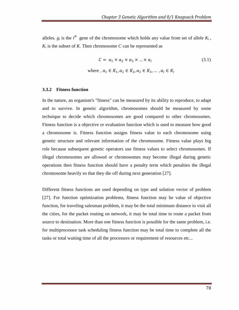
3.3.2 Fitness function

In the nature, an organism's "fitness" can be measured by its ability to reproduce, to adapt

and to survive. In genetic algorithm, chromosomes should be measured by some

technique to decide which chromosomes are good compared to other chromosomes.

Fitness function is a objective or evaluation function which is used to measure how good

a chromosome is. Fitness function assigns fitness value to each chromosome using

genetic structure and relevant information of the chromosome. Fitness value plays big

role because subsequent genetic operators use fitness values to select chromosomes. If

illegal chromosomes are allowed or chromosomes may become illegal during genetic

operations then fitness function should have a penalty term which penalties the illegal

chromosome heavily so that they die off during next generation [27].

Different fitness functions are used depending on type and solution vector of problem

[27]. For function optimization problems, fitness function may be value of objective

function, for traveling salesman problem, it may be the total minimum distance to visit all

the cities, for the packet routing on network, it may be total time to route a packet from

source to destination. More than one fitness function is possible for the same problem, i.e.

for multiprocessor task scheduling fitness function may be total time to complete all the

tasks or total waiting time of all the processors or requirement of resources etc...


79

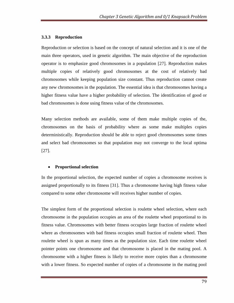
3.3.3 Reproduction

Reproduction or selection is based on the concept of natural selection and it is one of the

main three operators, used in genetic algorithm. The main objective of the reproduction

operator is to emphasize good chromosomes in a population [27]. Reproduction makes

multiple copies of relatively good chromosomes at the cost of relatively bad

chromosomes while keeping population size constant. Thus reproduction cannot create

any new chromosomes in the population. The essential idea is that chromosomes having a

higher fitness value have a higher probability of selection. The identification of good or

bad chromosomes is done using fitness value of the chromosomes.

Many selection methods are available, some of them make multiple copies of the,

chromosomes on the basis of probability where as some make multiples copies

deterministically. Reproduction should be able to reject good chromosomes some times

and select bad chromosomes so that population may not converge to the local optima

[27].

Proportional selection

In the proportional selection, the expected number of copies a chromosome receives is

assigned proportionally to its fitness [31]. Thus a chromosome having high fitness value

compared to some other chromosome will receives higher number of copies.

The simplest form of the proportional selection is roulette wheel selection, where each

chromosome in the population occupies an area of the roulette wheel proportional to its

fitness value. Chromosomes with better fitness occupies large fraction of roulette wheel

where as chromosomes with bad fitness occupies small fraction of roulette wheel. Then

roulette wheel is spun as many times as the population size. Each time roulette wheel

pointer points one chromosome and that chromosome is placed in the mating pool. A

chromosome with a higher fitness is likely to receive more copies than a chromosome

with a lower fitness. So expected number of copies of a chromosome in the mating pool


80

can be given by 𝑓/𝑓 where f is the fitness of particular chromosome and 𝑓 is the average

fitness of population [32].

Roulette wheel selection is widely used for maximization problems but it has two main

drawbacks. First drawback is that it can handle only maximization problem so

minimization problem must be converted into an equivalent maximization problem. If

fitness values may be negative then transformation from minimization to maximization

becomes more difficult. Second problem is that if a population contains a chromosome

having exceptionally better fitness compared to the rest of chromosomes in the

population then this chromosome occupies most of the roulette wheel area. Thus, almost

all the spinning of the roulette wheel is likely to choose the same chromosome, this may

result in the lost of genes diversity and population may converge to local optima [27].

Second problem can be avoided by the scaling of fitness, where fitness of each

chromosome is linearly mapped between a lower and an upper bound before marking the

roulette wheel.

Figure 3.1 Roulette Wheel Selection Method

Rank based Selection

Rank based selection uses fitness value of the chromosomes to sort chromosomes in to

ascending or descending order depending on the minimization or maximization problem.

Then it assigns reproduction probability and ranked fitness to each chromosome on the


81

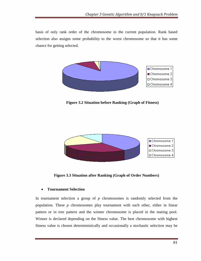
basis of only rank order of the chromosome in the current population. Rank based

selection also assigns some probability to the worst chromosome so that it has some

chance for getting selected.

Figure 3.2 Situation before Ranking (Graph of Fitness)

Figure 3.3 Situation after Ranking (Graph of Order Numbers)

Tournament Selection

In tournament selection a group of p chromosomes is randomly selected from the

population. These p chromosomes play tournament with each other, either in linear

pattern or in tree pattern and the winner chromosome is placed in the mating pool.

Winner is declared depending on the fitness value. The best chromosome with highest

fitness value is chosen deterministically and occasionally a stochastic selection may be


82

made [31]. Some times in the stochastic selection, instead of selecting only one

chromosome, a group of q chromosomes are declared winners and all the q chromosomes

are placed in the mating pool. This process is repeated till the mating pool has µ

chromosomes. Generally tournament is held between two chromosomes and it is known

as a binary tournament, p is called tournament size. It can handle minimization and

maximization problems without any transformation and it can be used with negative

fitness value also. More over its implementation is quite simple and efficient. One

drawback of the tournament selection is that worst chromosome can never be selected

because it is always looser if tournament is played deterministically.

Steady State Selection

In the steady state selection in every generation a few good chromosomes are selected for

creating new offspring. Then some bad chromosomes are removed and the new offspring

is placed. The rest of population survives to new generation.

Elitism

After crossover and mutation new population is generated. With the help of elitism we

can store the best found chromosomes. The remaining chromosomes are delivered for the

next generation. In this way we cannot lose best chromosomes.

3.3.4 Crossover

Crossover or recombination works as per the principle of sexual recombination. In

biological systems, recombination is a complex process that occurs between male and

female of same species. Two chromosomes are physically aligned, breakage occurs at

one or more location on each chromosome and homologous chromosome fragments are

exchanged before the breaks are repaired. Same concept is also applied in the genetic

algorithm. Two parent chromosomes are selected randomly from the mating pool, few

genes of the chromosomes are exchanged between these two parents and offspring are


83

produced. In general, crossover operator recombines two chromosomes so it is also

known as recombination.

Crossover is intelligent search operator that exploits the information acquired by the

parent chromosomes to generate new offspring [24]. If both the parents have same

genetic structure then offspring are just copies of the parent irrespective of cutting point

but if parents have different genetic structure then offspring are different then parents.

Thus, crossover is sampling process, which samples new points in the search space.

Better the sampling rate, more chances of getting solution. In biological system, new

child is produced by sexual crossing-over only. Thus, crossover should be performed

every time, so generally probability of crossover is very high like 1.00, 0.95, 0.90 etc...

Generally crossover operators are designed as per the encoding scheme [31]. The

crossover operator designed for binary encoding may not work with matrix encoding of

traveling salesman problem or edge recombination operator of permutation encoding. So

crossover is problem specific and for each problem, many types of crossover operators

are available, even one can design according to one's requirement [31]. Few of the well-

known crossover operators are discussed below.

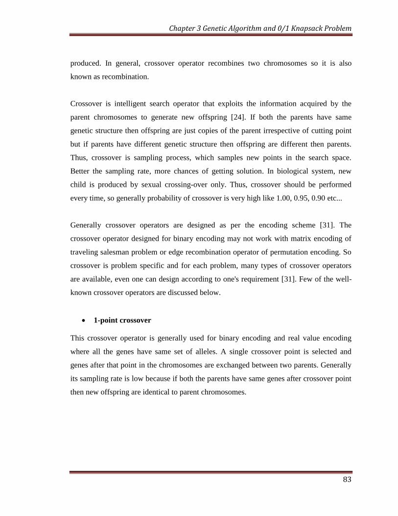
1-point crossover

This crossover operator is generally used for binary encoding and real value encoding

where all the genes have same set of alleles. A single crossover point is selected and

genes after that point in the chromosomes are exchanged between two parents. Generally

its sampling rate is low because if both the parents have same genes after crossover point

then new offspring are identical to parent chromosomes.


84

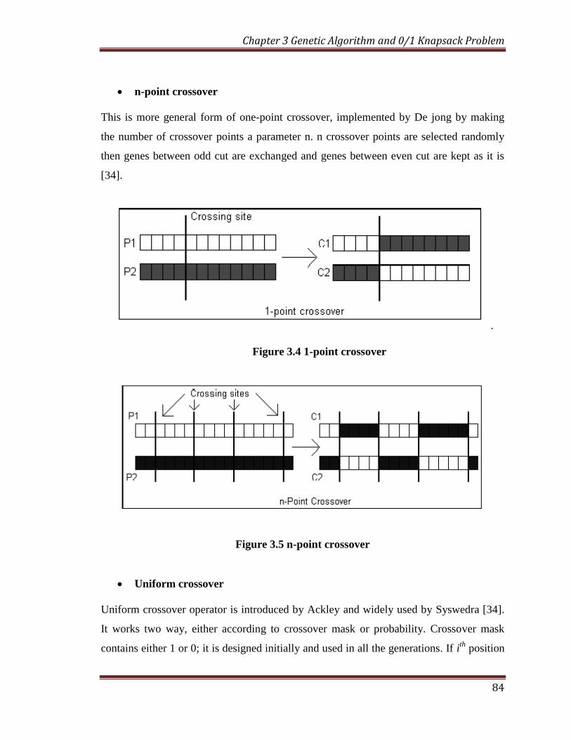
n-point crossover

This is more general form of one-point crossover, implemented by De jong by making

the number of crossover points a parameter n. n crossover points are selected randomly

then genes between odd cut are exchanged and genes between even cut are kept as it is

[34].

.

Figure 3.4 1-point crossover

Figure 3.5 n-point crossover

Uniform crossover

Uniform crossover operator is introduced by Ackley and widely used by Syswedra [34].

It works two way, either according to crossover mask or probability. Crossover mask

contains either 1 or 0; it is designed initially and used in all the generations. If ith

position


85

of mask contains 1 then ith

gene will be interchanged otherwise not. In the probability

approach, probability is used to decide whether the genes should be exchanged or not.

Generally gene exchange probability is uniform on all the genes.

Figure 3.6 Uniform crossover

3.3.5 Mutation

Some times in biological evolution, some genes are deficient. Some gene has allele value

that is not present in any of the parent chromosome but it appears in the child offspring,

which is mutation of gene. Sometimes due to mutation genes deficiency occurs and living

organism may suffer from some diseases but sometimes it is required to survive in

dynamic environment. So there is much confusion about role of mutation in biological

systems [31].

Mutation is secondary operator used in genetic algorithm to explore new points in the

search space. In the latter stages of a run, the population may converge in wrong direction

and stuck to the local optima. The effect of mutation is to reintroduce divergence into a

converging population [31]. Mutation operator selects one chromosome randomly from

the population, then selects some genes using mutation probability and flips that bit. So

mutation is a random operator that randomly alters some value. Mutation either explores

some new points in the search space and leads population to the global optima direction

or alters value of the best chromosome and losses knowledge acquired, till now. So


86

mutation should be used rarely, generally per gene probability of mutation is 0.001, 0.01,

0.02 etc...

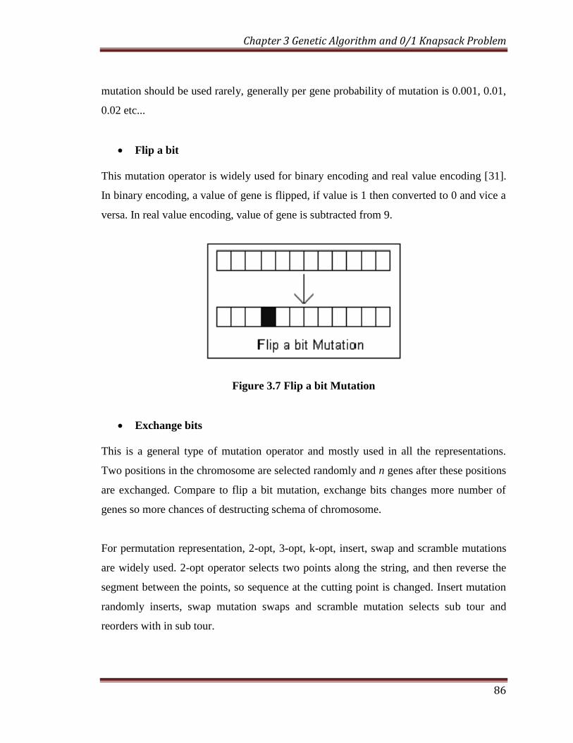
Flip a bit

This mutation operator is widely used for binary encoding and real value encoding [31].

In binary encoding, a value of gene is flipped, if value is 1 then converted to 0 and vice a

versa. In real value encoding, value of gene is subtracted from 9.

Figure 3.7 Flip a bit Mutation

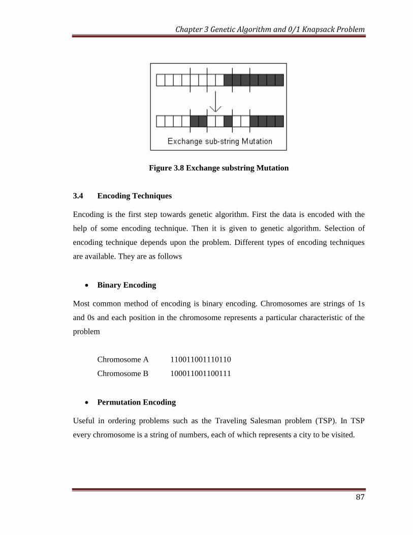
Exchange bits

This is a general type of mutation operator and mostly used in all the representations.

Two positions in the chromosome are selected randomly and n genes after these positions

are exchanged. Compare to flip a bit mutation, exchange bits changes more number of

genes so more chances of destructing schema of chromosome.

For permutation representation, 2-opt, 3-opt, k-opt, insert, swap and scramble mutations

are widely used. 2-opt operator selects two points along the string, and then reverse the

segment between the points, so sequence at the cutting point is changed. Insert mutation

randomly inserts, swap mutation swaps and scramble mutation selects sub tour and

reorders with in sub tour.


87

Figure 3.8 Exchange substring Mutation

3.4 Encoding Techniques

Encoding is the first step towards genetic algorithm. First the data is encoded with the

help of some encoding technique. Then it is given to genetic algorithm. Selection of

encoding technique depends upon the problem. Different types of encoding techniques

are available. They are as follows

Binary Encoding

Most common method of encoding is binary encoding. Chromosomes are strings of 1s

and 0s and each position in the chromosome represents a particular characteristic of the

problem

Chromosome A 110011001110110

Chromosome B 100011001100111

Permutation Encoding

Useful in ordering problems such as the Traveling Salesman problem (TSP). In TSP

every chromosome is a string of numbers, each of which represents a city to be visited.


88

Chromosome A 1 5 3 2 6 4 7 9 8

Chromosome B 8 5 6 7 2 3 1 4 9

Value Encoding

Used in problems where complicated values, such as real numbers, are used and where

binary encoding would not suffice. Good for some problems, but often necessary to

develop some specific crossover and mutation techniques for these chromosomes.

Chromosome A 1.235 5.323 0.454 2.321 2.454

Chromosome B (left), (back), (left), (right), (forward)

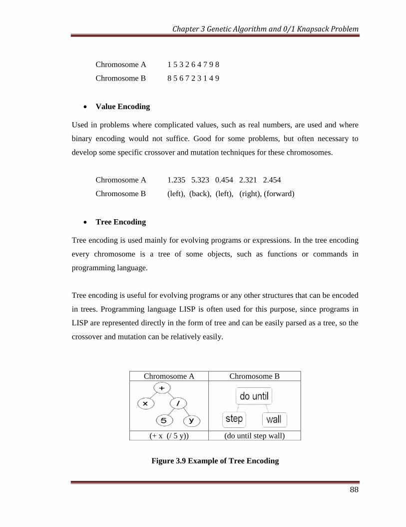
Tree Encoding

Tree encoding is used mainly for evolving programs or expressions. In the tree encoding

every chromosome is a tree of some objects, such as functions or commands in

programming language.

Tree encoding is useful for evolving programs or any other structures that can be encoded

in trees. Programming language LISP is often used for this purpose, since programs in

LISP are represented directly in the form of tree and can be easily parsed as a tree, so the

crossover and mutation can be relatively easily.

Figure 3.9 Example of Tree Encoding

Chromosome A Chromosome B

(+ x (/ 5 y)) (do until step wall)


89

3.5 Simple Genetic Algorithm (Non-Overlapping Populations)

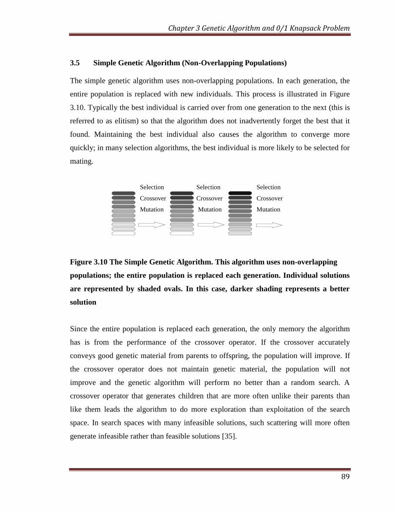
The simple genetic algorithm uses non-overlapping populations. In each generation, the

entire population is replaced with new individuals. This process is illustrated in Figure

3.10. Typically the best individual is carried over from one generation to the next (this is

referred to as elitism) so that the algorithm does not inadvertently forget the best that it

found. Maintaining the best individual also causes the algorithm to converge more

quickly; in many selection algorithms, the best individual is more likely to be selected for

mating.

Selection Selection Selection

Crossover Crossover Crossover

Mutation Mutation Mutation

Figure 3.10 The Simple Genetic Algorithm. This algorithm uses non-overlapping

populations; the entire population is replaced each generation. Individual solutions

are represented by shaded ovals. In this case, darker shading represents a better

solution

Since the entire population is replaced each generation, the only memory the algorithm

has is from the performance of the crossover operator. If the crossover accurately

conveys good genetic material from parents to offspring, the population will improve. If

the crossover operator does not maintain genetic material, the population will not

improve and the genetic algorithm will perform no better than a random search. A

crossover operator that generates children that are more often unlike their parents than

like them leads the algorithm to do more exploration than exploitation of the search

space. In search spaces with many infeasible solutions, such scattering will more often

generate infeasible rather than feasible solutions [35].


90

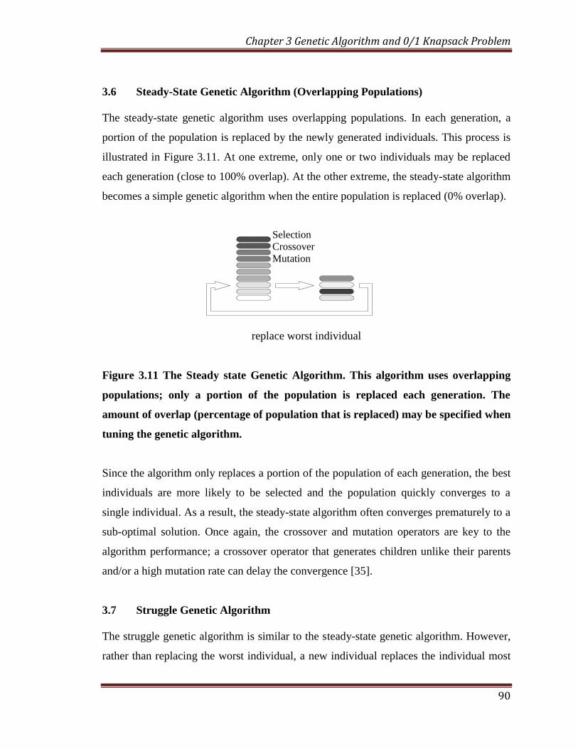
3.6 Steady-State Genetic Algorithm (Overlapping Populations)

The steady-state genetic algorithm uses overlapping populations. In each generation, a

portion of the population is replaced by the newly generated individuals. This process is

illustrated in Figure 3.11. At one extreme, only one or two individuals may be replaced

each generation (close to 100% overlap). At the other extreme, the steady-state algorithm

becomes a simple genetic algorithm when the entire population is replaced (0% overlap).

Selection

Crossover

Mutation

replace worst individual

Figure 3.11 The Steady state Genetic Algorithm. This algorithm uses overlapping

populations; only a portion of the population is replaced each generation. The

amount of overlap (percentage of population that is replaced) may be specified when

tuning the genetic algorithm.

Since the algorithm only replaces a portion of the population of each generation, the best

individuals are more likely to be selected and the population quickly converges to a

single individual. As a result, the steady-state algorithm often converges prematurely to a

sub-optimal solution. Once again, the crossover and mutation operators are key to the

algorithm performance; a crossover operator that generates children unlike their parents

and/or a high mutation rate can delay the convergence [35].

3.7 Struggle Genetic Algorithm

The struggle genetic algorithm is similar to the steady-state genetic algorithm. However,

rather than replacing the worst individual, a new individual replaces the individual most


91

similar to it, but only if the new individual has a score better than that of the one to which

it is most similar. This requires the definition of a measure of similarity (often referred to

as a distance function). The similarity measure indicates how different two individuals

are, either in terms of their actual structure (the genotype) or of their characteristics in the

problem-space (the phenotype).

Selection

Mutation

Crossover

replace most-similar if new is better

Figure 3.12 The Struggle Genetic Algorithm. This algorithm is similar to the steady-

state algorithm, but whereas the steady-state algorithm uses a “replace worst”

strategy for inserting new individuals into the population, the struggle algorithm

uses a form of “replace most similar”.

The struggle genetic algorithm was developed by Griininger in order to adaptively

maintain diversity among solutions [Griininger 96]. As noted previously, if allowed to

evolve long enough, both the simple and the steady-state algorithms converge to a single

solution; eventually the population consists of many copies of the same individual. Once

the population converges in this manner, mutation is the only source of additional

change. Conversely, a population evolving with a struggle algorithm maintains different

solutions (as defined by the similarity measure) long after a simple or steady-state

algorithm would have converged. Unlike other niching methods such as sharing or

crowding [Goldberg and Richardson 87] [Mahfoud 95][De Jong 75], the struggle

algorithm requires no niching radius or other parameters to tune the speciation


92

performance. The struggle algorithm is similar to deterministic crowding and shares some

characteristics of restricted tournament selection.

If the similarity function is properly defined, the struggle algorithm maintains diversity

extremely well. However, like the other genetic algorithms, performance is tightly

coupled to the genetic operators. For example, if the crossover operator has a very low

probability of generating good individuals when mating between or across species (as

defined by the similarity measure), the algorithm will fail. If the mutation rate is too high,

the algorithm will perform only as well as a random search [35].

3.8 Pseudocode of Simple Genetic Algorithm

The Pseudocode of Simple Genetic Algorithm is as given below:

1. Choose initial population (usually random)

2. Repeat (until terminated)

• Evaluate each individual's fitness

• Prune population (typically all; if not, then the worst)

• Select pairs to mate from best-ranked individuals

• Replenish population (using selected pairs)

- Apply crossover operator

- Apply mutation operator

• Check for termination criteria

(number of generations, amount of time, minimum fitness threshold satisfied,

fitness has reached a plateau, other)

- Loop, if not terminating


93

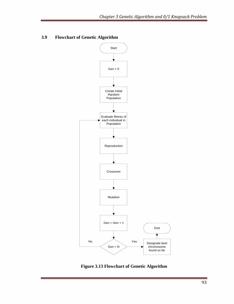
3.9 Flowchart of Genetic Algorithm

Start

Gen = 0

Create Initial

Random

Population

Evaluate fitness of

each individual in

Population

Reproduction

Crossover

Mutation

Gen = Gen + 1

Gen = N

Designate best

chromosome

found so far

End

YesNo

Figure 3.13 Flowchart of Genetic Algorithm


94

3.10 Why genetic algorithm works?

There is no strong mathematical background that tells that why and how genetic

algorithm works but John Holland has developed schemata theorem which gives idea of

why genetic algorithm works [24]. A schema is a similarity template describing a subset

of strings with similarities at certain string positions [32]. Suppose we use binary

encoding then chromosome C can have either 0 or 1 and for either of two, we add

notation don't care and denote it as *. If length of chromosome C is l then C has {0, 1}l

dimensions and C can be represented as.

C = a1a2a3…al (3.2)

This ai is known as allele and each of the ai represents a single binary feature which may

take a value 1 or 0.

3.10.1 Schema theorem

Let us denote a schema as a H it and it is taken from the three letter alphabet V = {0, l,

*}. The order of a schema H, denoted as O (H), is the number of fixed positions present

in the template [32]. For the schema H = 011 *1*, the order of the schema H is 4, O (H) =

4 because only 4 bits are fixed bits and others are don't care. The defining length of a

schema H, denoted as (H), is the distance between the first and last fixed bits in the

string position. For the schema H = 011 *1*, the defining length (H) = 5 because the

first fixed bit is at 1st position and last fixed bit is at 6

th bit position so distance between

them is 5. Now let us consider the effect of all three genetic operators one by one.

The effect of reproduction on the population can be determined easily. Suppose at a given

time t, there are m copies of a particular schema H in the population set P (t). In

reproduction, a chromosome is selected according to its fitness. We can say that a

chromosome C1 gets selected with the probability 𝑝𝑖 =𝑓𝑖

𝑓𝑗 . If population size is µ and


95

generation gap is 1 then the number of copies of schema H in the next generation is given

by

( )( , 1) ( , ). .

i

f Hm H m H t

f (3.3)

where f (H) is the average fitness of all the chromosomes representing schema H at time

t. If we denote average fitness of population as f then f = if

then the above

equation can be rewritten as

( )( , 1) ( , ). .

f Hm H m H t

f

(3.4)

We can say that if average fitness of schema H is more than average fitness of

population, that means if ( )f H f then schema H will get more number of copies in the

next generation otherwise less number of copies than current generation.

Crossover is a structured yet randomized information exchange between chromosomes.

Crossover creates new structures with a minimum disruption of schema. A lower bound

on crossover survival probability under simple Crossover is Ps = 1 - (H)/ (l - 1), since

the schema is likely to be disrupted whenever a crossing site within the defining length is

selected from the l - 1 possible sites. If a crossover itself performed by the probability Pc

at a mating, the" survival probability may be given by the expression

( )1

1s c

HP P

l

(3.5)

Mutation is the random alteration of a single position with a probability Pm. In order for

a schema H to survive, all of the specified positions must themselves survive. Therefore,

a single allele survives with probability (1 - Pm), and since each of the mutations are

statistically Independent, a particular schema survives when each of the O (H) fixed

positions within the schema survives. So schema survival probability is (1 - Pm) O (H)

. If


96

Pm << 1, the schema, survival probability may be approximated by the expression 1 - O

(H). Pm.

We, therefore conclude that a, particular schema H receives an expected number of

copies in the next generation under reproduction, crossover, and mutation is given by

( ) ( )( , 1) ( , ). 1 ( ).

1

f H Hm H t M H t Pc O H Pm

f l

(3.6)

3.11 Advantages of Genetic Algorithm

3.11.1 Global Search Methods

Gas search for the function optimum starting from a population of points of the function

domain, not a single one. This characteristic suggests that Gas are global search methods.

They can, in fact, climb many peaks in parallel, reducing the probability of finding local

minima, which is one of the drawbacks of traditional optimization methods.

3.11.2 Blind Search Methods

Gas only uses the information about the objective function. They do not require

knowledge of the first derivative or any other auxiliary information, allowing a number of

problems to be solved without the need to formulate restrictive assumptions. For this

reason, Gas are often called blind search methods.

3.11.3 Gas use probabilistic transition rules during iterations, unlike the traditional

methods that use fixed transition rules. This makes them more robust and applicable to a

large range of problems.


97

3.11.4 Gas can be easily used in parallel machines

Since in real world design optimization problems, most computational time is spent in

evaluating a solution, with multiple processors all solutions in a population can be

evaluated in a distributed manner. This reduces the overall computational time

substantially.

3.12 Weak points of Genetic algorithm

Genetic algorithm is based on natural evolution and generally it is tested, compared and

measured on empirical results because stochastic information plays big role in the genetic

algorithm. More over mathematical foundation of genetic algorithm is not so strong.

Some of the weak points are discussed below.

3.12.1 Lacking in Standardization

There is no standard formula that tells whether genetic algorithm will really work or not

for a given problem. Procedure of genetic algorithm can be easily changed and modified,

so one use according to one's desire and requirement. High level of flexibility is available

but it makes confusion. Behavior of genetic algorithm depends on the characteristics of

problem and varies from problem to problem. More over there is no clear-cut guidelines

about setting of various parameters; some are defined roughly but not well. Following

questions are still not satisfactory answered.

Which model should be used?

Which model converges fast in the right direction?

Which encoding scheme is the best? Binary, gray code, decimal encoding, etc ... [32]

Which reproduction technique is best? Tournament, roulette wheel, etc ...


98

Which crossover method is the best? I-point, uniform, etc ...

What should be the population size?

What should be the mutation and crossover rate?

Whether genetic algorithm really gives good result or not? [36]

3.12.2 Problem with encoding techniques

Generally binary encoding and decimal encoding is used but they have drawbacks.

Domain of binary encoding is 0 and 1 only; whereas domain of decimal encoding is 0 to

9. Binary encoding has a problem of hamming distance. Phenotype of 0111 is 7 and

phenotype of 1000 is 8. So in the phenotype they have the small difference but in

genotype they are completely different and they have maximum distance. So it is difficult

to convert strings like 0111 to 1000 or vice a versa, using crossover and mutation. In

decimal encoding a gene can have any value from 0 to 9 so allele loss probability is high

which is less in the case of binary encoding.

3.12.3 Problem with Reproduction

Reproduction is used to reproduce or to select good chromosomes for the successive

genetic operations and generations. It should make multiple copies of relatively good

chromosomes at the cost of bad chromosomes. If it fails to do so then convergence in the

right direction is not possible [32]. Roulette wheel is widely used for reproduction as

discussed in Section 3.3.3. Suppose there are five chromosomes with fitness of

5,15,20,25,35 then selection probability of best chromosome 5th

, is 0.35 which is less.

This situation even becomes worst when population contains hundreds of chromosomes

and with small differences in fitness value. More over it is difficult to convert

minimization problem into maximization. Suppose in minimization problem, population


99

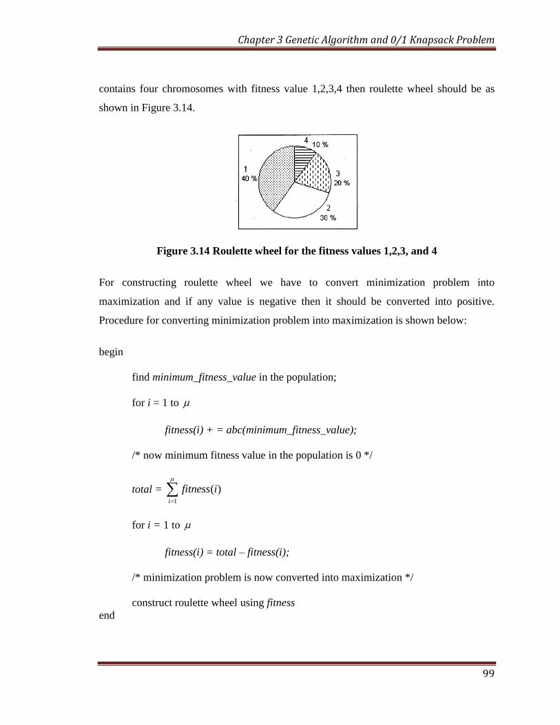
contains four chromosomes with fitness value 1,2,3,4 then roulette wheel should be as

shown in Figure 3.14.

Figure 3.14 Roulette wheel for the fitness values 1,2,3, and 4

For constructing roulette wheel we have to convert minimization problem into

maximization and if any value is negative then it should be converted into positive.

Procedure for converting minimization problem into maximization is shown below:

begin

find minimum_fitness_value in the population;

for i = 1 to

fitness(i) + = abc(minimum_fitness_value);

/* now minimum fitness value in the population is 0 */

total = 1

( )i

fitness i

for i = 1 to

fitness(i) = total – fitness(i);

/* minimization problem is now converted into maximization */

construct roulette wheel using fitness

end


100

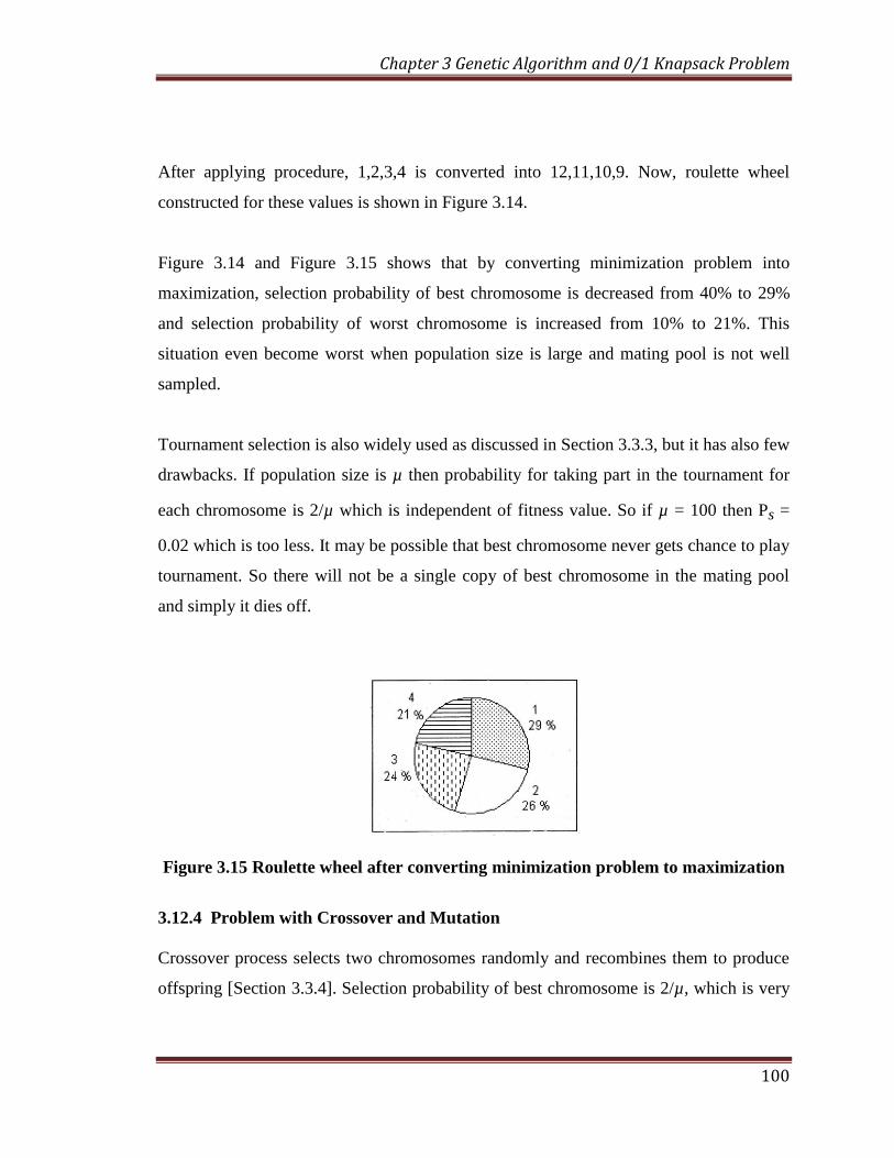
After applying procedure, 1,2,3,4 is converted into 12,11,10,9. Now, roulette wheel

constructed for these values is shown in Figure 3.14.

Figure 3.14 and Figure 3.15 shows that by converting minimization problem into

maximization, selection probability of best chromosome is decreased from 40% to 29%

and selection probability of worst chromosome is increased from 10% to 21%. This

situation even become worst when population size is large and mating pool is not well

sampled.

Tournament selection is also widely used as discussed in Section 3.3.3, but it has also few

drawbacks. If population size is µ then probability for taking part in the tournament for

each chromosome is 2/µ which is independent of fitness value. So if µ = 100 then Ps =

0.02 which is too less. It may be possible that best chromosome never gets chance to play

tournament. So there will not be a single copy of best chromosome in the mating pool

and simply it dies off.

Figure 3.15 Roulette wheel after converting minimization problem to maximization

3.12.4 Problem with Crossover and Mutation

Crossover process selects two chromosomes randomly and recombines them to produce

offspring [Section 3.3.4]. Selection probability of best chromosome is 2/µ, which is very


101

less [Section 3.3.3]. More over what should be the crossover rate? Should we perform

crossover on the entire population set or should we copy some of the chromosomes

directly?

Mutation is generally referred as a random search [Section 3.3.5]. What should be the

mutation rate? If mutation is like flip a bit then mutation probability is per gene but if

mutation is like exchange sub-string or insert, then how to treat mutation probability.

Where mutation does good job? In the early phase or later phase of the genetic algorithm

run?.

3.12.5 Problem with Allele loss

Generally it is said that sometimes genetic algorithm stuck to local minima. But allele

loss problem is more serious than local minima. If mutation rate is high then allele loss

probability is low but it is random search and if mutation rate is low then allele loss

probability high but it may stuck to local minima.

3.13 0/1 Knapsack Problem

0/1 Knapsack is the problem of selecting objects from a collection. Given say n objects,

their weights and values (profit), and also maximum capacity of a knapsack, the problem

is to find a permutation of objects, so that their total weight is less than or equal to the

given capacity and total value is maximum, with the condition that each object should be

either taken or not taken, we cannot take a part of an object. This problem is well known

to be hard and no polynomial-time algorithm exists to solve this optimally. So this falls

under NP-Complete set of problems. Genetic Algorithms are made use recently to find an

approximately optimal solution for this problem [37].

3.13.1 Definition

The classical knapsack problem is defined as follows:


102

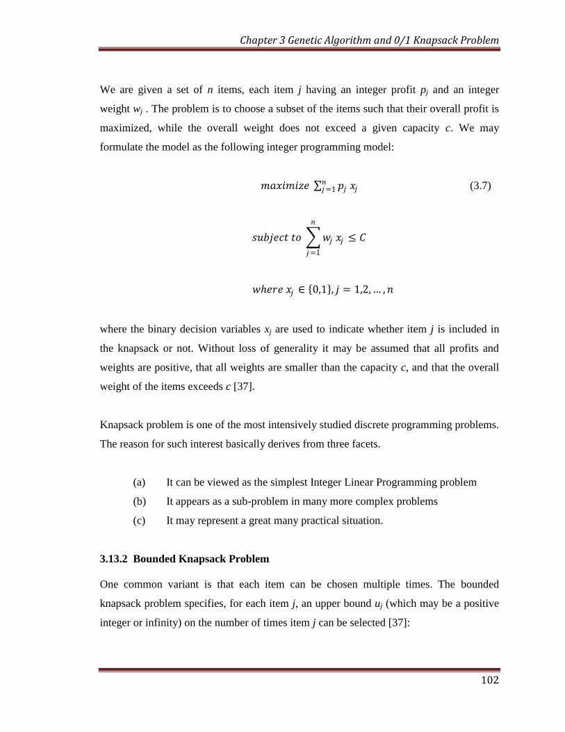
We are given a set of n items, each item j having an integer profit pj and an integer

weight wj . The problem is to choose a subset of the items such that their overall profit is

maximized, while the overall weight does not exceed a given capacity c. We may

formulate the model as the following integer programming model:

𝑚𝑎𝑥𝑖𝑚𝑖𝑧𝑒 𝑝𝑗𝑛𝑗=1 𝑥𝑗 (3.7)

𝑠𝑢𝑏𝑗𝑒𝑐𝑡 𝑡𝑜 𝑤𝑗

𝑛

𝑗=1

𝑥𝑗 ≤ 𝐶

𝑤𝑕𝑒𝑟𝑒 𝑥𝑗 ∈ 0,1 , 𝑗 = 1,2, … , 𝑛

where the binary decision variables xj are used to indicate whether item j is included in

the knapsack or not. Without loss of generality it may be assumed that all profits and

weights are positive, that all weights are smaller than the capacity c, and that the overall

weight of the items exceeds c [37].

Knapsack problem is one of the most intensively studied discrete programming problems.

The reason for such interest basically derives from three facets.

(a) It can be viewed as the simplest Integer Linear Programming problem

(b) It appears as a sub-problem in many more complex problems

(c) It may represent a great many practical situation.

3.13.2 Bounded Knapsack Problem

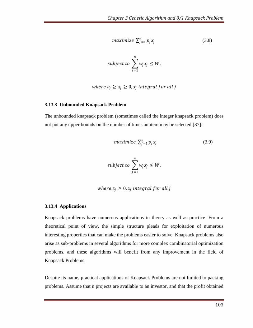
One common variant is that each item can be chosen multiple times. The bounded

knapsack problem specifies, for each item j, an upper bound uj (which may be a positive

integer or infinity) on the number of times item j can be selected [37]:


103

𝑚𝑎𝑥𝑖𝑚𝑖𝑧𝑒 𝑝𝑗𝑥𝑗𝑛𝑗=1 (3.8)

𝑠𝑢𝑏𝑗𝑒𝑐𝑡 𝑡𝑜 𝑤𝑗𝑥𝑗 ≤ 𝑊,

𝑛

𝑗=1

𝑤𝑕𝑒𝑟𝑒 𝑢𝑗 ≥ 𝑥𝑗 ≥ 0, 𝑥𝑗 𝑖𝑛𝑡𝑒𝑔𝑟𝑎𝑙 𝑓𝑜𝑟 𝑎𝑙𝑙 𝑗

3.13.3 Unbounded Knapsack Problem

The unbounded knapsack problem (sometimes called the integer knapsack problem) does

not put any upper bounds on the number of times an item may be selected [37]:

𝑚𝑎𝑥𝑖𝑚𝑖𝑧𝑒 𝑝𝑗𝑥𝑗𝑛𝑗=1 (3.9)

𝑠𝑢𝑏𝑗𝑒𝑐𝑡 𝑡𝑜 𝑤𝑗𝑥𝑗 ≤ 𝑊,

𝑛

𝑗=1

𝑤𝑕𝑒𝑟𝑒 𝑥𝑗 ≥ 0, 𝑥𝑗 𝑖𝑛𝑡𝑒𝑔𝑟𝑎𝑙 𝑓𝑜𝑟 𝑎𝑙𝑙 𝑗

3.13.4 Applications

Knapsack problems have numerous applications in theory as well as practice. From a

theoretical point of view, the simple structure pleads for exploitation of numerous

interesting properties that can make the problems easier to solve. Knapsack problems also

arise as sub-problems in several algorithms for more complex combinatorial optimization

problems, and these algorithms will benefit from any improvement in the field of

Knapsack Problems.

Despite its name, practical applications of Knapsack Problems are not limited to packing

problems. Assume that n projects are available to an investor, and that the profit obtained


104

from the jth

project is pj, j= 1,…,n. It costs wj to invest in project j, and only C dollars are

available. An optimal investment plan may be found by solving a 0-1 Knapsack Problem.

Another application appear in a restaurant, where a person has to choose K courses,

without surpassing the amount of C calories, his diet prescribes. Assuming that there are

Ni dishes to choose among for each course i=1,…,k and wij is the nutritive value while pij

is a rating saying how well each dish tastes. Then an optimal meal may be found by

solving the Multiple-Choice Knapsack Problem.

The Bin-packing Problem has been applied for cutting iron bars in order to minimize the

number of bars used each day. Here wi is the length of each piece demanded, while C is

the length of each bar, as delivered from the factory.

Apart from these simple illustrations we should mention the following major

applications: Problems in cargo loading, Cutting Stock, budget control, and financial

management may be formulated as Knapsack Problems, where the specific model

depends on the side constraints present.

Sinha and Zoltners proposed to use multiple-choice Knapsack problems to select which

components should be linked in series in order to maximize fault tolerance. Diffie and

Hellman designed a public cryptography scheme whose security relies on the difficulty of

solving the Subset-sum problem. Martello and Toth mention that two-processor

scheduling problems may be solved as Subset-sum problem. Finally Bin-Packing

problem may be used for packing envelopes with a fixed weight limit.

The most theoretical applications either appear where a general problem is transformed to

a Knapsack problem or where the Knapsack problem appears as sub-problem [37].


105

3.13.5 Hardness

Suppose you want to invest-all or in part- a capital of C dollars and you are considering n

possible investments. Let pj be the profit you expect from investment j, and wj the amount

of dollars it requires. It is self-evident that the optimal solution of the knapsack problem

above will indicate the best possible choice of investments.

At this point you may be stimulated to solve the problem. A naive approach would be to

program a computer to examine all possible binary vectors x, selecting the best of those

which satisfy the constraint. Unfortunately, the number of such vectors is 2n, so even a

hypothetical computer, capable of examining one billion vectors per second, would

require more than 30 years for n=60, more than 60 years for n=61, ten centuries for n =

65, and so on. However, specialized algorithms can, in most cases, solve a problem with

n = 100000 in a few seconds on a mini computer.

Documents

Chapter 3. Genetic algorithm and 0/1 Knapsack Problem 3.1 ...shodhganga.inflibnet.ac.in/bitstream/10603/78747/10/10_chapter 3.pdf · Chapter 3 Genetic Algorithm and 0/1 Knapsack Problem