Embed Size (px)
Citation preview
Chapter 3. Gradients & Optimization Methods
By: FARHAD FARADJI, Ph.D.Assistant Professor,
Electrical Engineering,K.N. Toosi University of Technology
http://wp.kntu.ac.ir/faradji/BSS.htm
References:Independent Component Analysis, A. Hyvärinen, J. Karhunen, E. Oja, John Wiley & Sons, 2001

Chapter Contents3.0. Introduction
3.1. Vector and matrix gradients
3.2. Learning rules for unconstrained optimization
3.3. Learning rules for constrained optimization
Independent Component Analysis Chapter 3. Gradients & Optimization Methods 2
3.0. Introduction
3.1. Vector and matrix gradients
3.2. Learning rules for unconstraineedd ooppttiimmization
3.3. Learning rules for constrainedd ooppttiimmiizzaation
Independent Component Analysis Chapter 3. Gradients & Optimization Methods 2
3.0. Introductiono The main task in the ICA problem,
formulated in Chapter 1,is to estimate a separating matrix W
that will give us the independent components.
o W cannot generally be solved in closed form,we cannot write it as some function of the sample or training set,
whose value could be directly evaluated.
o Instead, the solution method is based oncost functions, also calledobjective functions orcontrast functions.
o Solutions W to ICA are foundat the minima or maxima of these functions.
Independent Component Analysis Chapter 3. Gradients & Optimization Methods 3
o The main task in the ICA problem,formulated in Chapter 1,
is to estimate a separating mmaattrriixx Wthat will give us the inddeeppeenddeenntt components.
o W cannot generally be solved in closeeedd form,we cannot write it ass ssssoommmmee ffffuunnnnccttttiiooonn oooof tthee ssample or training set,
whose vaaaalllluueeeee ccoouuuuldd beee ddddiiiirreeeeccttllyyyyy eeeevvvvaaluaatttteeddd....
o Instead, the solutionn mmmmmmeeeetthhhhooooddddd iiiisssss bbbbaaaaassssseeeeddddd ooooonnnnnncost functions, also cccaaaaallllllleeeeedddddobjective functions orcontrast functions.
o Solutions W to ICA are foundat the minima or maxima of these functions.
Independent Component Analysis Chapter 3. Gradients & Optimization Methods 3
3.0. Introductiono Several possible ICA cost functions will be discussed in next chapters.
o In general, statistical estimation is largely based onoptimization of cost functions.
o Minimization of multivariate functions,possibly under some constraints on the solutions,
is the subject of optimization theory.
o In this chapter, we discusssome typical iterative optimization algorithms andtheir properties.
o Mostly, the algorithms are based onthe gradients of the cost functions.
Independent Component Analysis Chapter 3. Gradients & Optimization Methods 4
o Several possible ICA cost functions will be discussed in next chapters.
o In general, statistical estimation is largely based onoptimization of cost functionss..
o Minimization of multivariate fuunncctioonss,,possibly under some constrainttttsss oooonnnn the solutions,
is the subject of oooppppptttttiiiimmmmiiiizzzzaaaaattttiiiiooooonnnnn tttthhhheeeeeooooorrrrryyyyy....
o In this chapterr,, wwwwweeee dddissccccuuuusssssssssssome typical iteraaaaattttttiiiiivvvvveee oooooppppptttttiiiiimmmmmiiiizzzzzaaaatttttiiioooonnnnn aaaaaallllgggggooooorrrrritttthhhhmmmmsssss aaaaanndtheir properties.
o Mostly, the algorithms are based onthe gradients of the cost functions.
Independent Component Analysis Chapter 3. Gradients & Optimization Methods 4
3.0. Introductiono Therefore, we review
vector and matrix gradients, andthe most typical ways to solve
unconstrained and constrained optimization problemswith gradient-type learning algorithms.
Independent Component Analysis Chapter 3. Gradients & Optimization Methods 5
o Therefore, we review vector and matrix gradients, andthe most typical ways to solvee
unconstrained and consttrraaiinned ooppttimization problemswith gradient-type learning alggorithms.
Independent Component Analysis Chapter 3. Gradients & Optimization Methods 5
Chapter Contents3.0. Introduction
3.1. Vector and matrix gradients
3.2. Learning rules for unconstrained optimization
3.3. Learning rules for constrained optimization
Independent Component Analysis Chapter 3. Gradients & Optimization Methods 6
3.0. Introduction
3.1. Vector and matrix gradients
3.2. Learning rules for unconstraineedd ooppttiimmization
3.3. Learning rules for constrainedd ooppttiimmiizzaation
Independent Component Analysis Chapter 3. Gradients & Optimization Methods 6

3.1. Vector and matrix gradients
o Consider a scalar valued function g of m variables:
w is a column vector.
o Assuming the function g is differentiable,its vector gradient with respect to w is
the m-dimensional column vector of partial derivatives:
Independent Component Analysis Chapter 3. Gradients & Optimization Methods 7
3.1.1. Vector gradiento Consider a scalar valued function g of m variables:
w is a column vector.
o Assuming the ffunction gg iisss ddddiiffffffffeeerrrrreeennnnttiiiiaaaabbbbbbllleeee,its vector ggrrraaddddiieeenntt wwiiitttthhhh reeesspppeecctttt ttooo wwww iss
the m-dimensiionnnnnal cccolllluummnn veccttttoor ooffffff pppaarrttttiiialllll dddderivatives:
Independent Component Analysis Chapter 3. Gradients & Optimization Methods 7
3.1.1. Vector gradient
3.1. Vector and matrix gradients
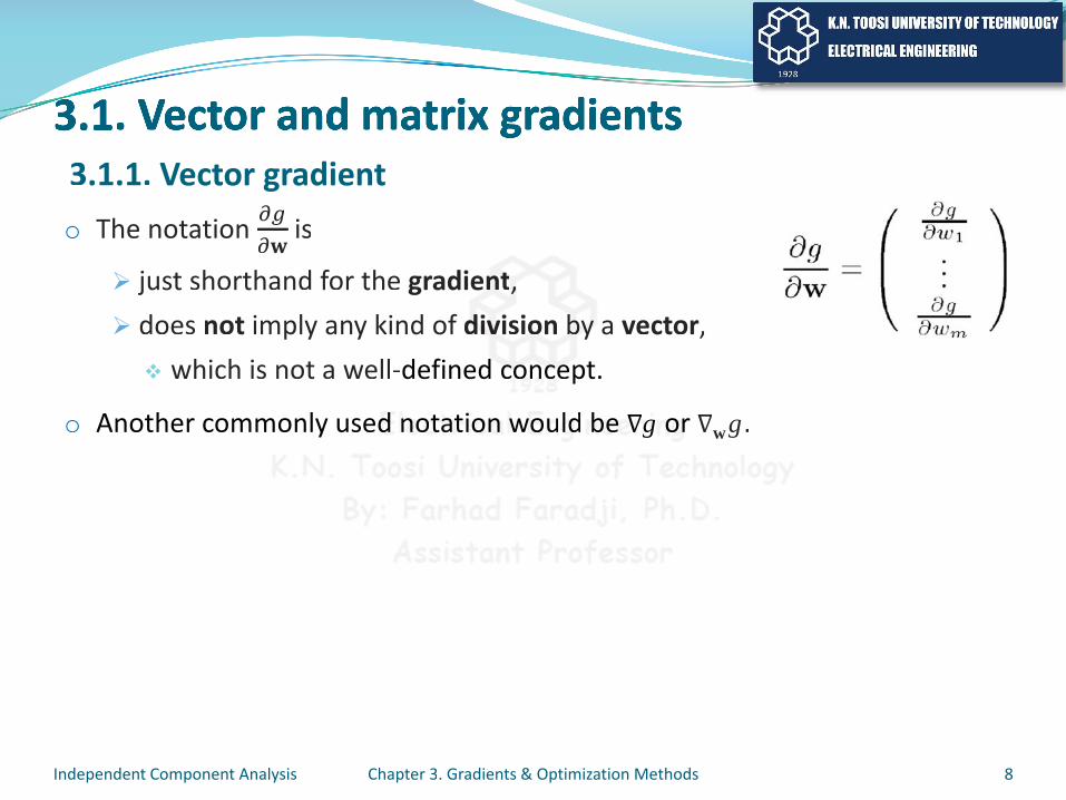
o The notation is
just shorthand for the gradient,does not imply any kind of division by a vector,
which is not a well-defined concept.
o Another commonly used notation would be g or wg.
Independent Component Analysis Chapter 3. Gradients & Optimization Methods 8
3.1.1. Vector gradiento The notation is
just shorthand for the gradienntt,,does not imply any kind of ddiivvisioon bbyy a vector,
which is not a well-defined ccoooonnncccceept.
o Another commonly useddd nnnnnooooootttttaaaaatttttiiiioooooonnnn wwwwwooooouuuuuullllllddddd bbbbbbeeeeee ggggg ooooorrrr wg.
Independent Component Analysis Chapter 3. Gradients & Optimization Methods 8
3.1.1. Vector gradient

3.1. Vector and matrix gradients
o In some iteration methods, we use second-order gradients.
o We define the second-order gradient of a function g with respect to w as:
o This is:an m×m matrix
whose elements are second-order partial derivatives.called the Hessian matrix of the function g(w).always symmetric.
Independent Component Analysis Chapter 3. Gradients & Optimization Methods 9
3.1.1. Vector gradiento In some iteration methods, we use second-order gradients.
o We define the second-order graddiieenntt ooff a function g with respect to w as:
o This is:an m×m matrix
whose elements are second-order partial derivatives.called the Hessian matrix of the function g(w).always symmetric.
Independent Component Analysis Chapter 3. Gradients & Optimization Methods 9
3.1.1. Vector gradient
3.1. Vector and matrix gradients
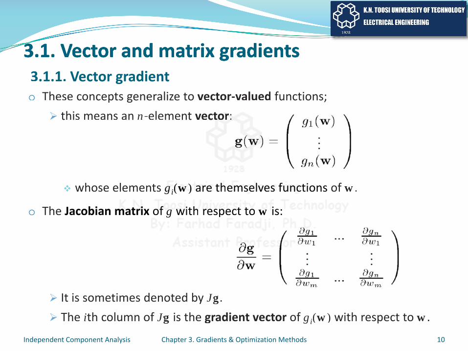
o These concepts generalize to vector-valued functions;this means an n-element vector:
whose elements gi(w) are themselves functions of w.
o The Jacobian matrix of g with respect to w is:
It is sometimes denoted by Jg.The ith column of Jg is the gradient vector of gi(w) with respect to w.
Independent Component Analysis Chapter 3. Gradients & Optimization Methods 10
3.1.1. Vector gradiento These concepts generalize to vector-valued functions;
this means an n-element vecttoorr::
whose elements gggiiiii((((wwwww))))) aaaaarrrreeee tttthhhhhheeeemmmmmsssssseeeeellvvvvvveeeeesssss fffffuuuunnnnncccccttions of w.
o The Jacobian mmmmaaaattttrrriiiixxx oofff gg wwwwiiittthhhh rrrreeeeesssspppeeeeeccctttt ttttooooo wwww is:
It is sometimes denoted by JgJJ .The ith column of JgJJ is the gradient vector of gi(w) with respect to w.
Independent Component Analysis Chapter 3. Gradients & Optimization Methods 10
3.1.1. Vector gradient
3.1. Vector and matrix gradients
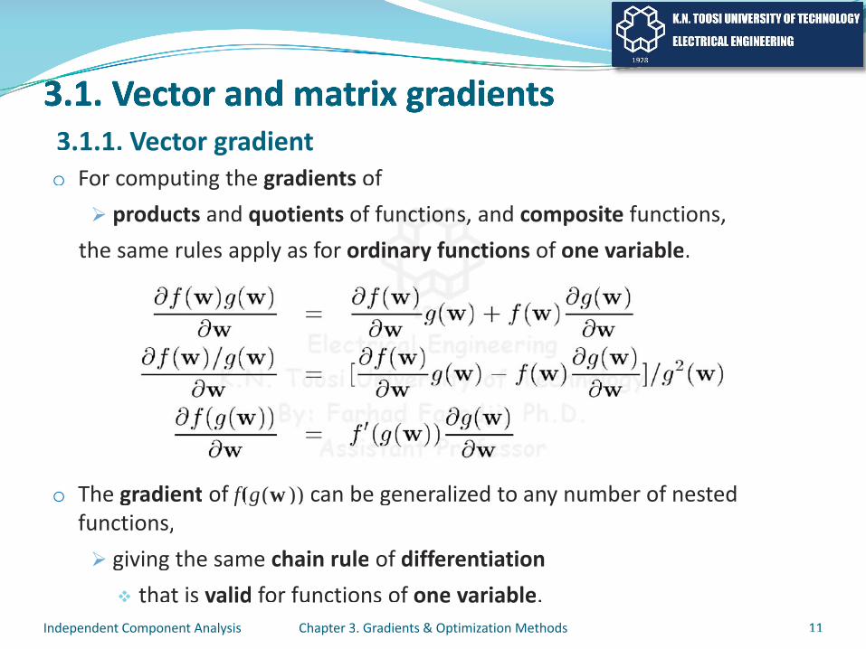
o For computing the gradients ofproducts and quotients of functions, and composite functions,
the same rules apply as for ordinary functions of one variable.
o The gradient of f(g(w)) can be generalized to any number of nested functions,
giving the same chain rule of differentiationthat is valid for functions of one variable.
Independent Component Analysis Chapter 3. Gradients & Optimization Methods 11
3.1.1. Vector gradiento For computing the gradients of
products and quotients of funnccttiioonnss,, and composite functions,the same rules apply as for ordiinnaarry fuunnccttions of one variable.
o The gradient of f(ff g(w)) can be generalized to any number of nested functions,
giving the same chain rule of differentiationthat is valid for functions of one variable.
Independent Component Analysis Chapter 3. Gradients & Optimization Methods 11
3.1.1. Vector gradient
3.1. Vector and matrix gradients
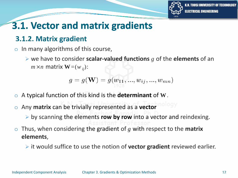
o In many algorithms of this course,we have to consider scalar-valued functions g of the elements of an m×n matrix W=(wij):
o A typical function of this kind is the determinant of W.
o Any matrix can be trivially represented as a vectorby scanning the elements row by row into a vector and reindexing.
o Thus, when considering the gradient of g with respect to the matrixelements,
it would suffice to use the notion of vector gradient reviewed earlier.
Independent Component Analysis Chapter 3. Gradients & Optimization Methods 12
3.1.2. Matrix gradiento In many algorithms of this course,
we have to consider scalar-vaalluueedd ffuunctions g of the elements of an m×n matrix W=(wij):
o A typical function of thisss kkkkiiiinnnnnddddd iiiiissss tttttthhhhheeeee dddddeeeeetttttteeeeerrrrrrmmmmmmiiiiinnnnnaaaaannnnnttttt oof W.
o Any matrix cannnn bbbbeee ttttrrrivviiiiaallllllllyyy rrrreeepppprrrreeeeesseeennnnntteeeedddd aaaaass aaaaa veeeeccttttooooorrrrby scanning the eelllleeeeemmennntttssss rrrooowwww bbbbyy rrrooowww iiiiinnnntttttoo aaa vvveeeccccttttor and reindexing.
o Thus, when considering the graddient of g wiiith respect to the matrixelements,
it would suffice to use the notion of vector gradient reviewed earlier.
Independent Component Analysis Chapter 3. Gradients & Optimization Methods 12
3.1.2. Matrix gradient
3.1. Vector and matrix gradients
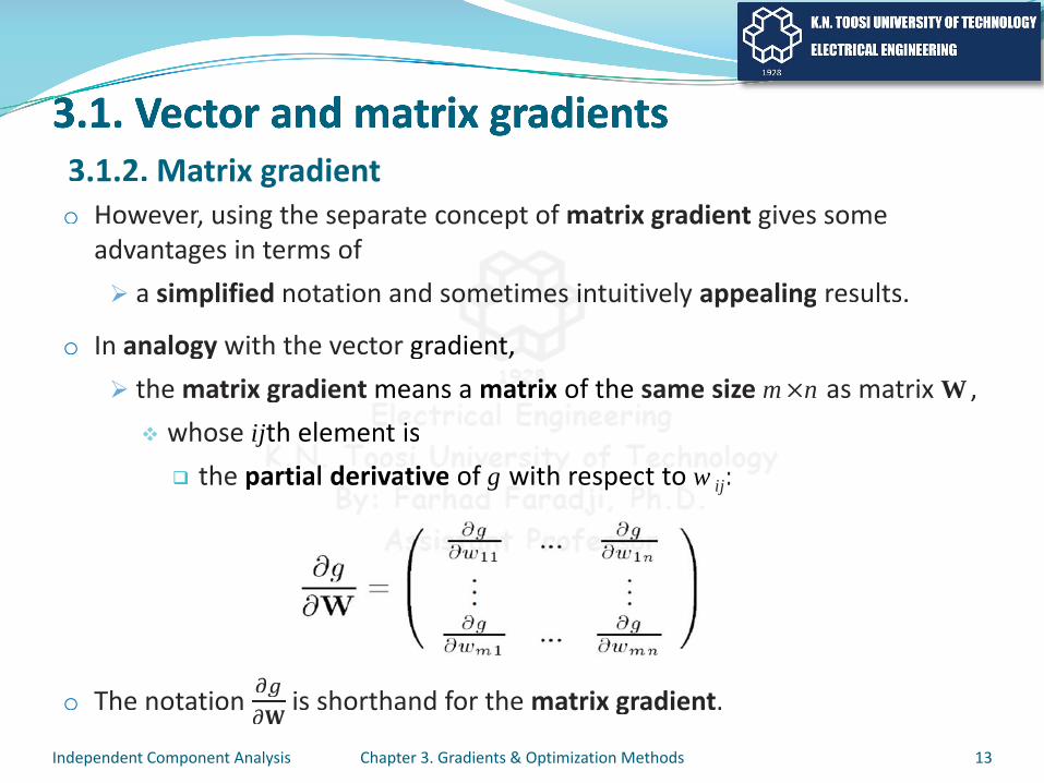
o However, using the separate concept of matrix gradient gives some advantages in terms of
a simplified notation and sometimes intuitively appealing results.
o In analogy with the vector gradient,the matrix gradient means a matrix of the same size m×n as matrix W,
whose ijth element isthe partial derivative of g with respect to wij:
o The notation is shorthand for the matrix gradient.
Independent Component Analysis Chapter 3. Gradients & Optimization Methods 13
3.1.2. Matrix gradiento However, using the separate concept of r matrix gradient gives some
advantages in terms ofa simplified notation and soommeettimmeess iintuitively appealing results.
o In analogy with the vector gradient,the matrix gradient mmeans a mmaaatttrrriiiixx oooff tthe same size m×n as matrix W,
whose ijjtth eeleemennttttt jj iiisthe partttiiiaalll ddeeerrriiivaatttiveee off ggggg wwwiiitthhhh rreeessspeecccttt tttooo wwij:
o The notation is shorthand for the matrix gradient.
Independent Component Analysis Chapter 3. Gradients & Optimization Methods 13
3.1.2. Matrix gradient
3.1. Vector and matrix gradients
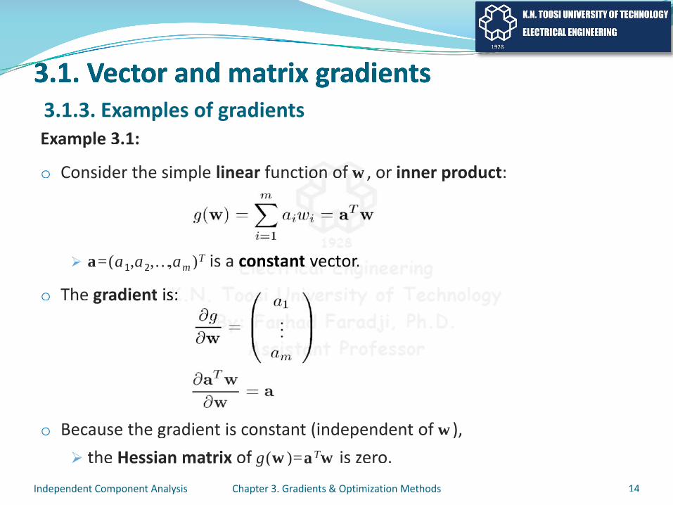
Example 3.1:
o Consider the simple linear function of w, or inner product:
a=(a1,a2,…,am)T is a constant vector.
o The gradient is:
o Because the gradient is constant (independent of w),the Hessian matrix of g(w)=aTw is zero.
Independent Component Analysis Chapter 3. Gradients & Optimization Methods 14
3.1.3. Examples of gradientsExample 3.1:
o Consider the simple linear functioonn ooff ww, or inner product:
a=(a1,a2,…,am)T is a cccooooonnnnnsssttttaaaaannnnntttt vvvveeeecccctttooooorrrr..
o The gradient iss:::::
o Because the gradient is constant (independent of w),the Hessian matrix of g(w)=aTwTT is zero.
Independent Component Analysis Chapter 3. Gradients & Optimization Methods 14
3.1.3. Examples of gradients
3.1. Vector and matrix gradients
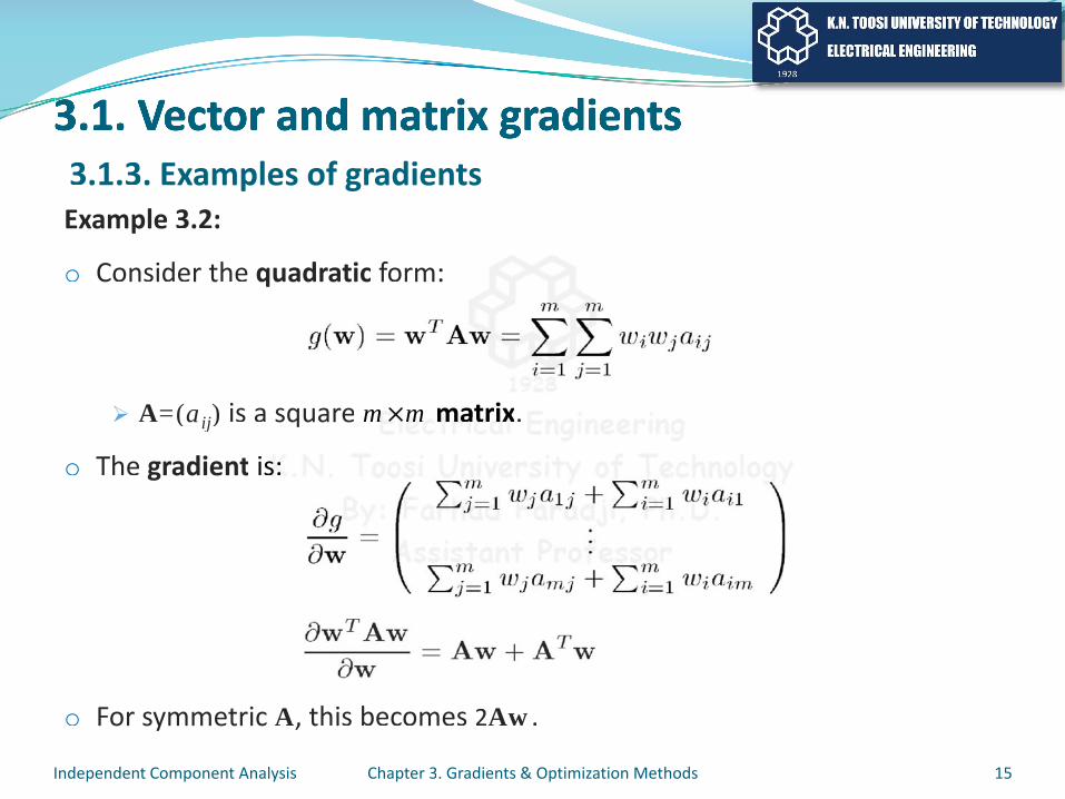
Example 3.2:
o Consider the quadratic form:
A=(aij) is a square m×m matrix.
o The gradient is:
o For symmetric A, this becomes 2Aw.
Independent Component Analysis Chapter 3. Gradients & Optimization Methods 15
3.1.3. Examples of gradientsExample 3.2:
o Consider the quadratic form:
A=(aij) is a square mmm×××××mmmmm mmmmmaaaaattttrrrriiiixxxx.
o The gradient iss:::::
o For symmetric A, A this becomes 2Aw.
Independent Component Analysis Chapter 3. Gradients & Optimization Methods 15
3.1.3. Examples of gradients
3.1. Vector and matrix gradients
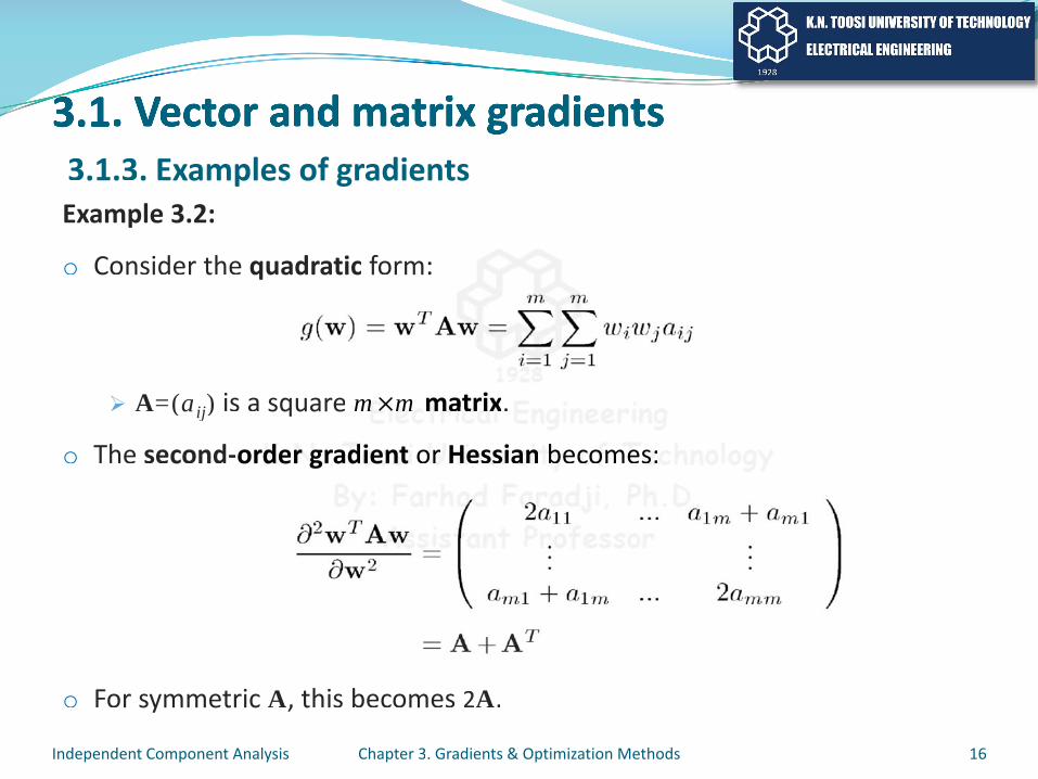
Example 3.2:
o Consider the quadratic form:
A=(aij) is a square m×m matrix.
o The second-order gradient or Hessian becomes:
o For symmetric A, this becomes 2A.
Independent Component Analysis Chapter 3. Gradients & Optimization Methods 16
3.1.3. Examples of gradientsExample 3.2:
o Consider the quadratic form:
A=(aij) is a square mmm×××××mmmmm mmmmmaaaaattttrrrriiiixxxx.
o The second-orrdddddeeeerrrr ggggrrraaddddddiiiieeeeennnnnttttt ooorrrrr HHHHHeeeeeesssssssssssiiiiiiaaaaannnnnn bbbbbbeeeeeccccoooooommmmeeeeesssss::::
o For symmetric A, A this becomes 2A.
Independent Component Analysis Chapter 3. Gradients & Optimization Methods 16
3.1.3. Examples of gradients
3.1. Vector and matrix gradients
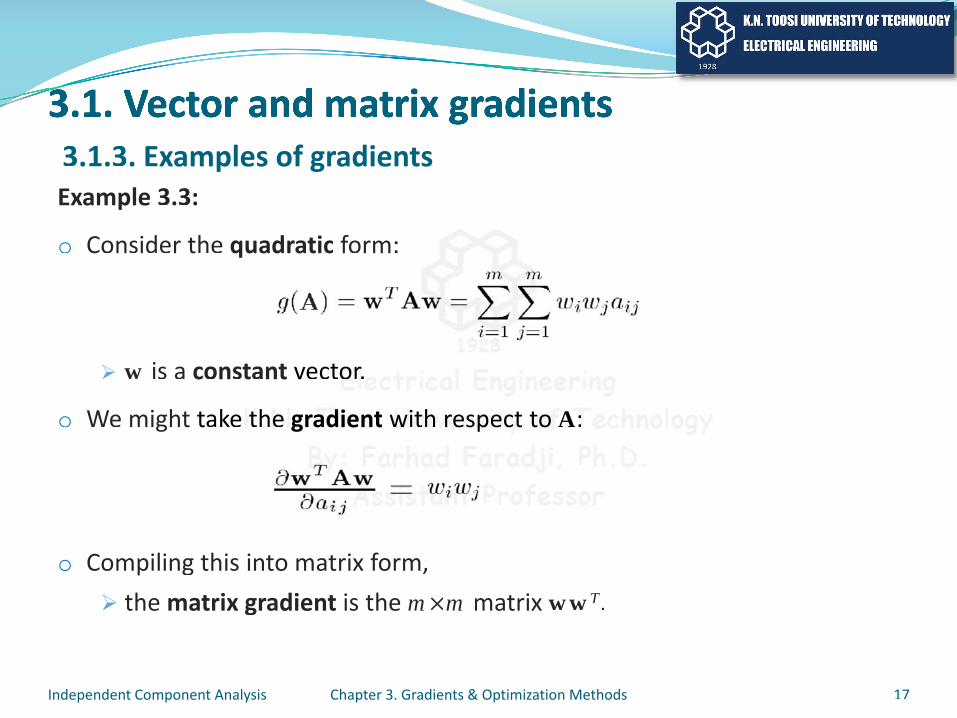
Example 3.3:
o Consider the quadratic form:
w is a constant vector.
o We might take the gradient with respect to A:
o Compiling this into matrix form,the matrix gradient is the m×m matrix wwT.
Independent Component Analysis Chapter 3. Gradients & Optimization Methods 17
3.1.3. Examples of gradientsExample 3.3:
o Consider the quadratic form:
w is a constant vectooorrrrr...
o We might takee ttttthhhheeee gggrraaadddddiiiieeeeennnnnttttt wwwwwiiiiittttthhhhhh rrrrrreeeeesssssspppppeeeeeccccctttttt ttttoooooo AAAA::
o Compiling this into matrix form,the matrix gradient is the m×m matrix wwT.
Independent Component Analysis Chapter 3. Gradients & Optimization Methods 17
3.1.3. Examples of gradients

3.1. Vector and matrix gradients
Example 3.4:
o In some ICA models,we must compute the matrix gradient of the determinant of a matrix.
o The determinantis a scalar function of the matrix elementsconsisting of multiplications and summations, and therefore
its partial derivatives are relatively simple to compute.
o Let us prove the following:If W is an invertible square m×m matrix with the determinant detW, then:
Independent Component Analysis Chapter 3. Gradients & Optimization Methods 18
3.1.3. Examples of gradientsExample 3.4:
o In some ICA models,we must compute the matriixx ggradiieenntt of the determinant of a matrix.
o The determinantis a scalar function ooofffff tttthhhhheeee mmmmmaaaaatttrrrrriiiiixx eeeellllleeeeemmmmmeeeeennnntttttsssssconsisting oooooffff mmmmmuuuulttiiipppppllliiiiccccaaaaatttttioooonnnnnsssss aaaaannnnnnddddd sssssuuuummmmmmmmmmmmaaaaattiiooooonnnnnsssss,,, aaaaannnnndddddd tttttthhhhheeeeeerrefore
its partial derivativessssss aaaaarrrree rrrrreeeelllllaaaaatttttiiiiivvvveeeelllllyy ssssiiiimmmmmpppppplllleeeee ttttto cccccooooommmmppppppuute.
o Let us prove the followinnngggg::::If W is an invertible square m×m matrix with the determinant detWt , then:
Independent Component Analysis Chapter 3. Gradients & Optimization Methods 18
3.1.3. Examples of gradients

3.1. Vector and matrix gradients
Example 3.4:
o This is a good example for showing thata compact formula is obtained using the matrix gradient.
o IfW were stacked into a long vector, andonly the vector gradient were used,
this result could not be expressed so simply.
Independent Component Analysis Chapter 3. Gradients & Optimization Methods 19
3.1.3. Examples of gradientsExample 3.4:
o This is a good example for showinngg tthhaatta compact formula is obtainneedd usingg tthe matrix gradient.
o IfW were stacked intooo aaaaa lllloooonnnnnggggg vvvvveeeeeccccctooooorrrr,,,, aaaaannnnnddddonly the veecccccttttooooorrrr ggrraaaaadddddiiiieeeeennnnnttttt wwwwweeeerrrrrreeeee uuuuussssseeeeddddd,,,
this result could not bbbbbbeeeee eeeexxxxppppprrrrreeeeesssssssssseeeeddddd sssssoooo ssssiiimmmmmmppppplllllyyyyy.
Independent Component Analysis Chapter 3. Gradients & Optimization Methods 19
3.1.3. Examples of gradients
3.1. Vector and matrix gradients
Example 3.4:
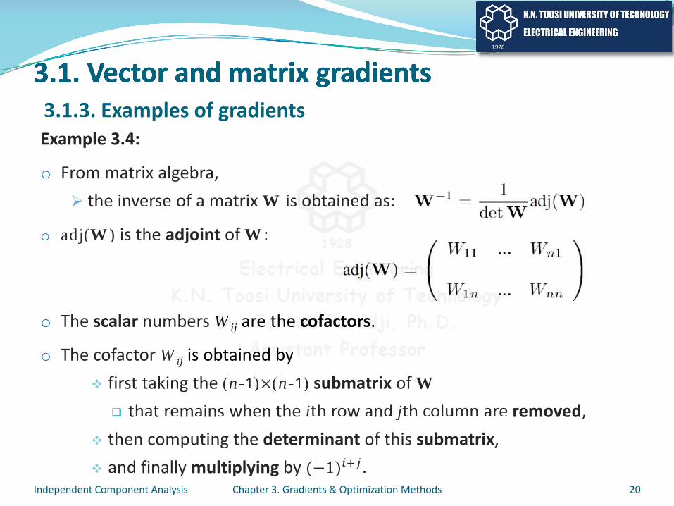
o From matrix algebra,the inverse of a matrix W is obtained as:
o adj(W) is the adjoint of W:
o The scalar numbers Wij are the cofactors.
o The cofactor Wij is obtained byfirst taking the (n-1)×(n-1) submatrix of W
that remains when the ith row and jth column are removed,then computing the determinant of this submatrix,and finally multiplying by ( 1) .
Independent Component Analysis Chapter 3. Gradients & Optimization Methods 20
3.1.3. Examples of gradientsExample 3.4:
o From matrix algebra,the inverse of a matrix W is oobbtaineedd aas:
o adj(W) is the adjoint of W:
o The scalar numbers WWWWWWijijijijijWWWWWWW aaaarrreeeee ttttthhhhheeeee ccccoooooffaaaaacccctttttooooorrrrssssss..
o The cofactor WijWW is obtainnnneeeeddddd bbbbbyyyyfirst taking the (n-1)×(n-1) submatrix of W
that remains when the ith row and jth column arejj removed,then computing the determinant of this submatrix,and finally multiplying by ( 1) .
Independent Component Analysis Chapter 3. Gradients & Optimization Methods 20
3.1.3. Examples of gradients

3.1. Vector and matrix gradients
Example 3.4:
o The determinant detW can also be expressedin terms of the cofactors:
o Row i can be any row, and the result is always the same.
o In the cofactors Wik,none of the matrix elements of the ith row appear, sothe determinant is a linear function of these elements.
o Taking now a partial derivative of above equation with respect to one of the elements, say, wij, gives:
o
Independent Component Analysis Chapter 3. Gradients & Optimization Methods 21
3.1.3. Examples of gradientsExample 3.4:
o The determinant detWt can also bbee eexxpprreessedin terms of the cofactors:
o Row i can be any row, annnddddd ttttthhhheeeee rrrrreeeeesssuuuuultttt iiiissssss aaaaalllllwwwwwaaaayyyyyssss ttttthhhhheeeee same.
o In the cofactorrsssss WWWWikikikkWWWWW ,,,none of the matrriiiiiixxxxxx eeeeelleeeemmmmmeeeeennnntttttssss oooooff ttthhhhhheeee iiiiiitttthhhhh rrrrooooowwww aaaappppppppeeeear, sothe determinant is a lllliiiinnnnneeeeeaaaaarrrrr fffffuuuuunnnnnccctttiiooooonnnnn oooooofffff ttttthhhhheeeeesssseeee elements.
o Taking now a partial derivative of above equation with respect to one of the elements, say, wij, gives:
o
Independent Component Analysis Chapter 3. Gradients & Optimization Methods 21
3.1.3. Examples of gradients
3.1. Vector and matrix gradients
Example 3.4:
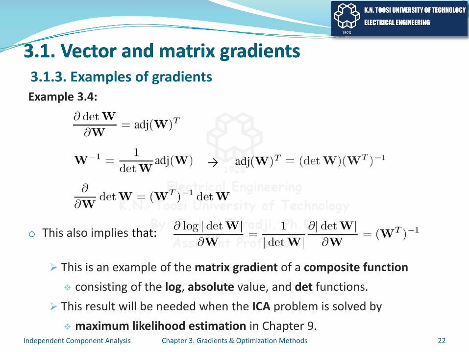
o This also implies that:
This is an example of the matrix gradient of a composite functionconsisting of the log, absolute value, and det functions.
This result will be needed when the ICA problem is solved bymaximum likelihood estimation in Chapter 9.
Independent Component Analysis Chapter 3. Gradients & Optimization Methods 22
3.1.3. Examples of gradientsExample 3.4:
o This also implies thattt:
This is an example of the matrix gradient of a composite functionconsisting of the log, absolute value, and det functions.
This result will be needed when the ICA problem is solved bymaximum likelihood estimation in Chapter 9.
Independent Component Analysis Chapter 3. Gradients & Optimization Methods 22
3.1.3. Examples of gradients
3.1. Vector and matrix gradients
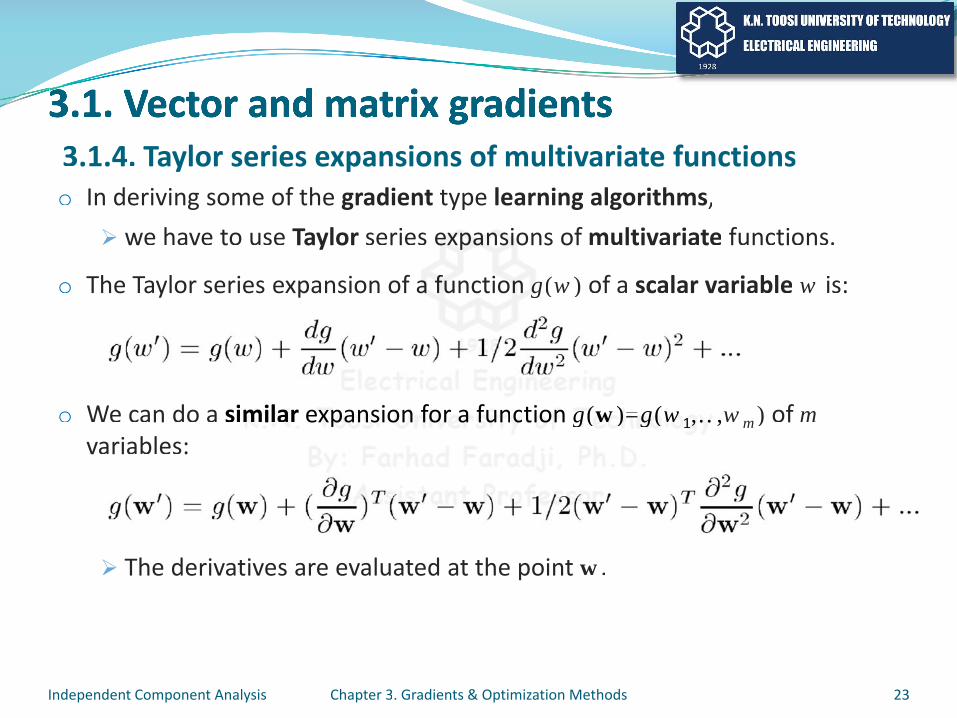
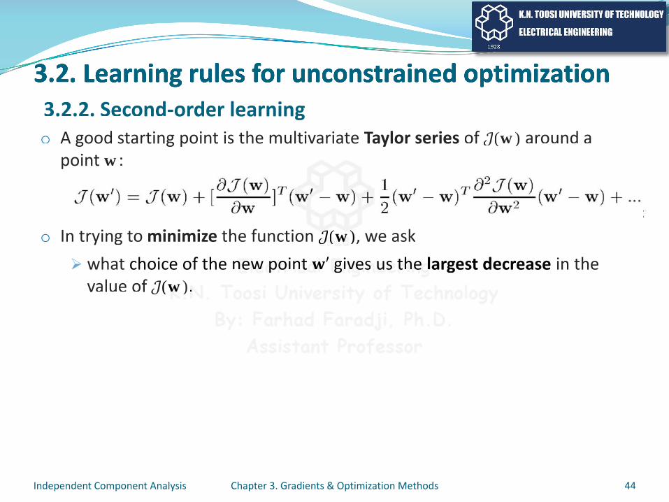
o In deriving some of the gradient type learning algorithms,we have to use Taylor series expansions of multivariate functions.
o The Taylor series expansion of a function g(w) of a scalar variable w is:
o We can do a similar expansion for a function g(w)=g(w1,…,wm) of mvariables:
The derivatives are evaluated at the point w.
Independent Component Analysis Chapter 3. Gradients & Optimization Methods 23
3.1.4. Taylor series expansions of multivariate functionso In deriving some of the gradient type learning algorithms,
we have to use Taylor series eexxppaannssiioons of multivariate functions.
o The Taylor series expansion of aa ffuunctioonn gg(w) of a scalar variable w is:
o We can do a siimmmmmilllllaaaarrrr eexxxxxpppppaaaaannnnnsssssioooonnnnn fffffoooooorrrrr aaaaa ffffuuuuunnnnccccccttiioooooonnnnn ggggg((((wwwwww))))))=====gggg((((((wwwww11111,,,,……………,wm) of mvariables:
The derivatives are evaluated at the point w.
Independent Component Analysis Chapter 3. Gradients & Optimization Methods 23
3.1.4. Taylor series expansions of multivariate functions
3.1. Vector and matrix gradients
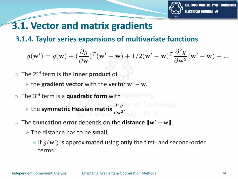
o The 2nd term is the inner product ofthe gradient vector with the vector .
o The 3rd term is a quadratic form with
the symmetric Hessian matrix .
o The truncation error depends on the distance .The distance has to be small,
if ( ) is approximated using only the first- and second-order terms.
Independent Component Analysis Chapter 3. Gradients & Optimization Methods 24
3.1.4. Taylor series expansions of multivariate functions
o The 2nd term is the inner producctt ooffthe gradient vector with the veeccccttttoooorrrrr .
o The 3rd term is a quadraaatttiiiccccc ffffooooorrrrmmmmm wwwwwiiiiithhhhh
the symmetttriiiicc HHHeeesssssiiiannn maaatttriixx .
o The truncation error depppeeeeennnnndddddsssss ooooonnnnn tttttthhhhhee dddddiiiisssssttttaaaaannnnncccceeeee .The distance has to be small,
if ( ) is approximated using only the first- and second-order terms.
Independent Component Analysis Chapter 3. Gradients & Optimization Methods 24
3.1.4. Taylor series expansions of multivariate functions
3.1. Vector and matrix gradients
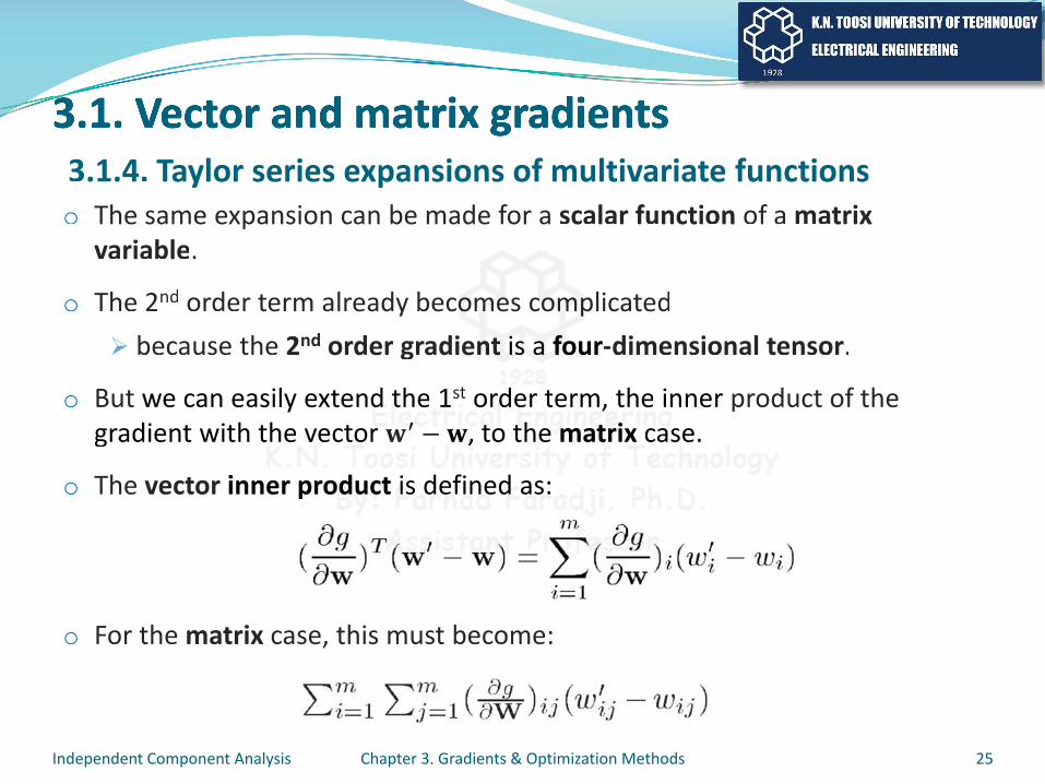
o The same expansion can be made for a scalar function of a matrixvariable.
o The 2nd order term already becomes complicatedbecause the 2nd order gradient is a four-dimensional tensor.
o But we can easily extend the 1st order term, the inner product of the gradient with the vector , to the matrix case.
o The vector inner product is defined as:
o For the matrix case, this must become:
Independent Component Analysis Chapter 3. Gradients & Optimization Methods 25
3.1.4. Taylor series expansions of multivariate functionso The same expansion can be made for a scalar function of a matrix
variable.
o The 2nd order term already becoommees ccoommpplicatedbecause the 2nd order gradienntt is a ffour-dimensional tensor.
o But we can easily extenddd tttthhe 11st oorrddddeeeerrr tteeerrrrmm, thheee inner product of the gradient with thhee veectorr ,, tttooo tthhhheee mmmmaaattttrrriiixxx ccaaasssse.
o The vector inner proodddduuuuccct iiissss dddeeeeefffiinnneeeeedddd aaaass:::
o For the matrix case, this must become:
Independent Component Analysis Chapter 3. Gradients & Optimization Methods 25
3.1.4. Taylor series expansions of multivariate functions

3.1. Vector and matrix gradients
o This is the sum of the products of corresponding elements,just like in the vectorial inner product.
o This can be nicely presented in matrix form.
o For any two matrices A and B, we have:
o Hence, for the first two terms in the Taylor series of a function g of a matrix variable:
Independent Component Analysis Chapter 3. Gradients & Optimization Methods 26
3.1.4. Taylor series expansions of multivariate functions
o This is the sum of the products ooff coorrreesspponding elements,just like in the vectorial inner pprrrroooodddduuuuct.
o This can be nicely preseennnntttteeeeeedddd iiiinnnnn mmmmmmaaaaaattttrrrrriiixxxxx ffffffooooorrrrrrmmmmmm...
o For any two maaaatttttrrrriiiiccceeeess AAAA aaaannnnnddddd BBBBB, wwwwweeee hhhhhaaavvvveeee::::
o Hence, for the first two terms in the Taylor series of a function g of a matrix variable:
Independent Component Analysis Chapter 3. Gradients & Optimization Methods 26
3.1.4. Taylor series expansions of multivariate functions
Chapter Contents3.0. Introduction
3.1. Vector and matrix gradients
3.2. Learning rules for unconstrained optimization
3.3. Learning rules for constrained optimization
Independent Component Analysis Chapter 3. Gradients & Optimization Methods 27
3.0. Introduction
3.1. Vector and matrix gradients
3.2. Learning rules for unconstrained optimization
3.3. Learning rules for constrainedd ooppttiimmiizzaation
Independent Component Analysis Chapter 3. Gradients & Optimization Methods 27
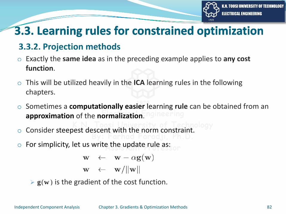
3.2. Learning rules for unconstrained optimization
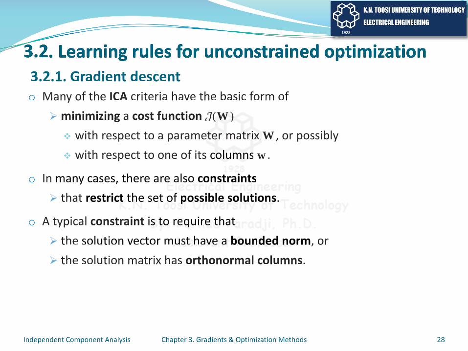
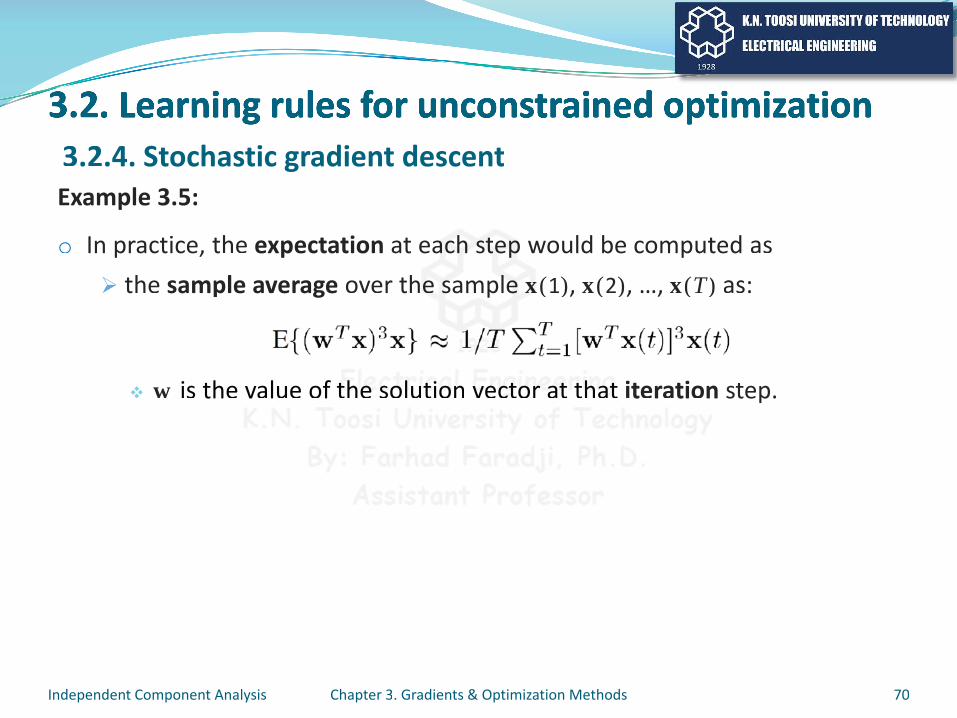
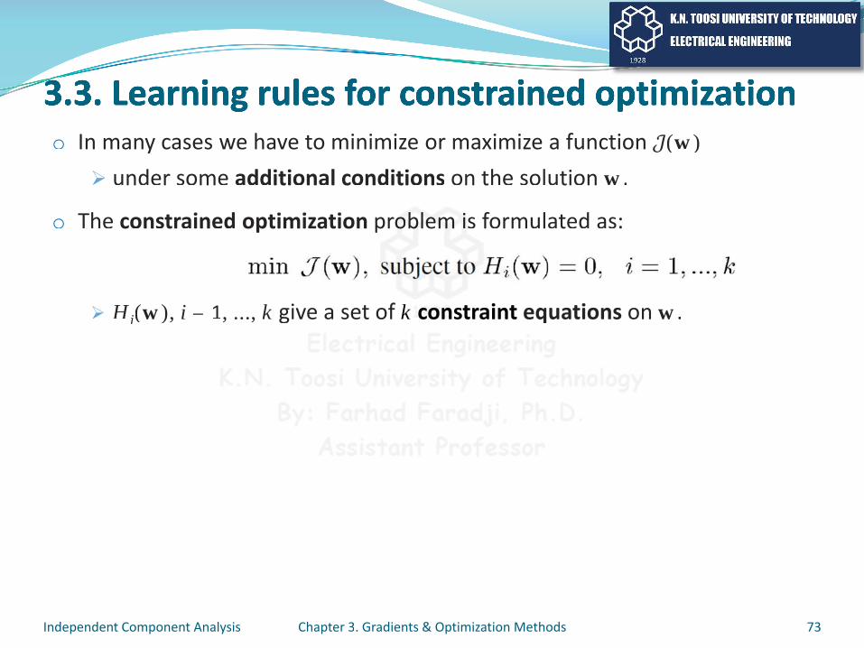
o Many of the ICA criteria have the basic form ofminimizing a cost function (W)
with respect to a parameter matrix W, or possiblywith respect to one of its columns w.
o In many cases, there are also constraintsthat restrict the set of possible solutions.
o A typical constraint is to require thatthe solution vector must have a bounded norm, orthe solution matrix has orthonormal columns.
Independent Component Analysis Chapter 3. Gradients & Optimization Methods 28
3.2.1. Gradient descento Many of the ICA criteria have the basic form of
minimizing a cost function ((WW))
with respect to a parameetteerr mattrriixx W, or possiblywith respect to one of its columns w.
o In many cases, there areee aaaaalssoo ccooooonnssttttraaaaiiinntsssssthat restrictttt thhhhheeee seeeettttt oof pppppoossssssssiibbbblee ssooolllluuuuttioonnssss.
o A typical constraint issssss tttttooooo rreeeeeqqqqquuuuuiiiirrrrreeee tttthhhhhaaaaattttthe solution vector mmmuuuuusssssttttt hhhhhaaaaavvvvveeeee aaaaaa bbooooouuuuunnnnndddddeeeeeddddd nnnnnnooooorrrm, orthe solution matrix has orthonormal columns.
Independent Component Analysis Chapter 3. Gradients & Optimization Methods 28
3.2.1. Gradient descent
3.2. Learning rules for unconstrained optimization
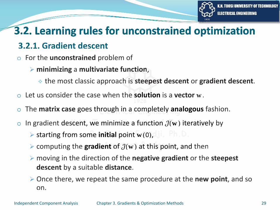
o For the unconstrained problem ofminimizing a multivariate function,
the most classic approach is steepest descent or gradient descent.
o Let us consider the case when the solution is a vector w.
o The matrix case goes through in a completely analogous fashion.
o In gradient descent, we minimize a function (w) iteratively bystarting from some initial point w(0),computing the gradient of (w) at this point, and thenmoving in the direction of the negative gradient or the steepestdescent by a suitable distance.Once there, we repeat the same procedure at the new point, and so on.
Independent Component Analysis Chapter 3. Gradients & Optimization Methods 29
3.2.1. Gradient descento For the unconstrained problem of
minimizing a multivariate funnccttiioonn,,the most classic approachh iiss ssteeeppeest descent or gradient descent.
o Let us consider the case when thee sollluuttion is a vector w.
o The matrix case goes thhrrrooooouuuuuggggghhhhh iiiiinnnnn aaaaa ccccoooommmmmppppppllllleeeeeetttteeeelllyyyyy aaaaannnnnaaaalogous fashion.
o In gradient dessccccceeeennnntttt,, wwwweeee mmmmmiiiiinnnnniimmmmmiiiiizzzzzeeeee aaaaaa fffffuuuuunnnncccccttttttiiooooonnnn (((((wwwww))))) iiiiittttteeeeerrrrraaaaaatttttiiivvvvveeeeeellyy bystarting from sommmmeeeeee iiinnnniittttiiiiaaaaalllll pppppooooiiiinnnnntt wwww(((((00000)))))),,,,computing the gradieeeennnnttttt ooooofffff ((((wwwww)))) aaattttt ttttthhhhhiiisssss ppppoooooiiinnnntttt, and thenmoving in the direction of the negative gradient or the steepestdescent by a suitable distance.Once there, we repeat the same procedure at the new point, and so on.
Independent Component Analysis Chapter 3. Gradients & Optimization Methods 29
3.2.1. Gradient descent
3.2. Learning rules for unconstrained optimization
o For t = 1, 2, …, we have the update rule:
with the gradient taken at the point w(t-1).
o The parameter (t) gives the length of the step in the negative gradient direction.
It is often called the step size or learning rate.
o Iteration is continued until it converges,which in practice happens when
the Euclidean distance between two consequent solutions, (t) w(t 1) , goes below some small tolerance level.
Independent Component Analysis Chapter 3. Gradients & Optimization Methods 30
3.2.1. Gradient descento For t = 1, 2, …, we have the update rule:
with the gradient taken at thhee ppooiinntt ww(t-1).
o The parameter (t) gives the lengtthhhhh oooofffff tthe step in the negative gradient direction.
It is often ccaaaaallllleeeedddd tthhheeee sssssttttteeeeepppp sssssiiiiizzzzzeeeeee oooooorrrrr llleeeeeeaaaarrrrrnnnnnniinnnnnnggggg rraaaaattttteeeee...
o Iteration is continueddddd uuuuunnnnttiiiil iiiittttt ccccooooonnnnvvvveerrrggggeeeeessss,which in practice happppppeeeeennnnssss wwwwwhhhhheeeeennn
the Euclidean distance between two consequent solutions, (t) w(t 1) , goes below some small tolerance level.
Independent Component Analysis Chapter 3. Gradients & Optimization Methods 30
3.2.1. Gradient descent

3.2. Learning rules for unconstrained optimization
o If there is no reason to emphasize the time or iteration step,a convenient shorthand notation will be used in presenting update rules of the preceding type.
o Denote the difference between the new and old value by:
o We can then write the rule either as:
o or even shorter as:
o The symbol is read “is proportional to”.
Independent Component Analysis Chapter 3. Gradients & Optimization Methods 31
3.2.1. Gradient descento If there is no reason to emphasize the time or iteration step,
a convenient shorthand notattiioonn wwiilll be used in presenting update rules of the preceding type.
o Denote the difference between tthhee neww and old value by:
o We can then wwwwrrrrriiitttteeee tttthheeee rrrruuuuulllleeeee eeeiiiittttthhhhheeeeerrrrr aaaaasss:::
o or even shorter as:
o The symbol is read “is proportional to”.
Independent Component Analysis Chapter 3. Gradients & Optimization Methods 31
3.2.1. Gradient descent
3.2. Learning rules for unconstrained optimization
o The vector on the left-hand side has the same direction as the gradient vector on the right-hand side, but
there is a positive scalar coefficient by which the length can be adjusted.
o In the upper version of the update rule, this coefficient is denoted by .
o In many cases, this learning rate is time dependent.
o A third way to write such update rules, in conformity with programming languages, is:
The symbol means substitution.Independent Component Analysis Chapter 3. Gradients & Optimization Methods 32
3.2.1. Gradient descent
o The vector on the left-hand sidee hhas thhee ssaame direction as the gradient vector on the right-hand side, butt
there is a positive scalar coefficcciieeennnnttt byy wwhich the length can be adjusted.
o In the upper versiiioon offff ttthhhhee upppdddddatttte rrulle, tthhhhiiiiiss cooeeefffffffffiiicciiiiieennttt iiissss dddddenoted by .
o In many cases, this learninnnnggg rrraaaaattteeee iiisss tttttimmmmeeee dddeeeepppppeeennnddddeeent.
o A third way to write such update rules, in conformity with programming languages, is:
The symbol means substitution.Independent Component Analysis Chapter 3. Gradients & Optimization Methods 32
3.2.1. Gradient descent
3.2. Learning rules for unconstrained optimization
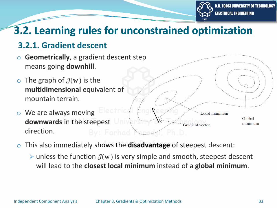
o Geometrically, a gradient descent step means going downhill.
o The graph of (w) is the multidimensional equivalent of mountain terrain.
o We are always moving downwards in the steepest direction.
o This also immediately shows the disadvantage of steepest descent:unless the function (w) is very simple and smooth, steepest descent will lead to the closest local minimum instead of a global minimum.
Independent Component Analysis Chapter 3. Gradients & Optimization Methods 33
3.2.1. Gradient descento Geometrically, a gradient descennt step
means going downhill.
o The graph of (w) is the multidimensional equivalent of mountain terrain.
o We are always moving downwards inn ttttthhhheeee ssssttteeeeeeppppeeeeesssssttttt direction.
o This also immediately shhoooowwwwwssss tttthhhhhheeeee dddddiiiisssaadddddvvvvvaaaaannnnntttttaaaaagggggeeeee oooof steepest descent:unless the function (w) is very simple and smooth, steepest descent will lead to the closest local minimum instead of a global minimum.
Independent Component Analysis Chapter 3. Gradients & Optimization Methods 33
3.2.1. Gradient descent

3.2. Learning rules for unconstrained optimization
o The method offers no way to escapefrom a local minimum.
o Nonquadratic cost functions may have many local maxima and minima.
o Therefore, good initial valuesare important in initializing the algorithm.
Independent Component Analysis Chapter 3. Gradients & Optimization Methods 34
3.2.1. Gradient descento The method offers no way to escaape
from a local minimum.
o Nonquadratic cost functions maayyyy have many local maxima and minima.
o Therefore, good initial vvvaaaaalllluuuueeeeessssare important iiiiinnnnn iinnnniiiitttiaallllliizzzziiinnnnnggggg the algorithm.
Independent Component Analysis Chapter 3. Gradients & Optimization Methods 34
3.2.1. Gradient descent
3.2. Learning rules for unconstrained optimization
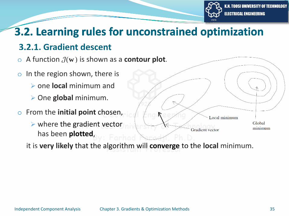
o A function (w) is shown as a contour plot.
o In the region shown, there isone local minimum andOne global minimum.
o From the initial point chosen, where the gradient vector has been plotted,
it is very likely that the algorithm will converge to the local minimum.
Independent Component Analysis Chapter 3. Gradients & Optimization Methods 35
3.2.1. Gradient descento A function (w) is shown as a conntour plot.
o In the region shown, there isone local minimum andOne global minimum.
o From the initial point chhhooooosssseeeeennnn,,,, where the gggggrrrraaddddiiiiennttttt vvvveeeeeccccctttttoorrrr has been plotttedd,,,,,,
it is very likely that the allgggggooorrrrriiittttthhhhmmmmm wwwwwiillllll cccccoooonnnnvvvveeerrrrgggggeeeee tttto the local minimum.
Independent Component Analysis Chapter 3. Gradients & Optimization Methods 35
3.2.1. Gradient descent
3.2. Learning rules for unconstrained optimization
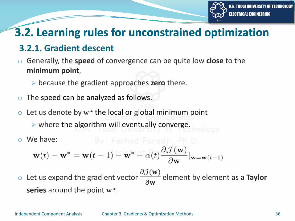
o Generally, the speed of convergence can be quite low close to the minimum point,
because the gradient approaches zero there.
o The speed can be analyzed as follows.
o Let us denote by w* the local or global minimum pointwhere the algorithm will eventually converge.
o We have:
o Let us expand the gradient vector ( )
element by element as a Taylorseries around the point w*.
Independent Component Analysis Chapter 3. Gradients & Optimization Methods 36
3.2.1. Gradient descento Generally, the speed of convergence can be quite low close to the
minimum point,because the gradient approaacchhees zzeerroo there.
o The speed can be analyzed as follows.
o Let us denote by w* thee llllooooccall ooorrrr gggloooobbbbaaal mmmmiiniimuuuumm ppointwhere the aaaallllggooooorrrrithhhmmmmm wiillll eeeevvvveeennnttuuaallllllyyyy connvvvveerrrggggee.
o We have:
o Let us expand the gradient vector ( )
element by element as a Taylorseries around the point w*.
Independent Component Analysis Chapter 3. Gradients & Optimization Methods 36
3.2.1. Gradient descent
3.2. Learning rules for unconstrained optimization
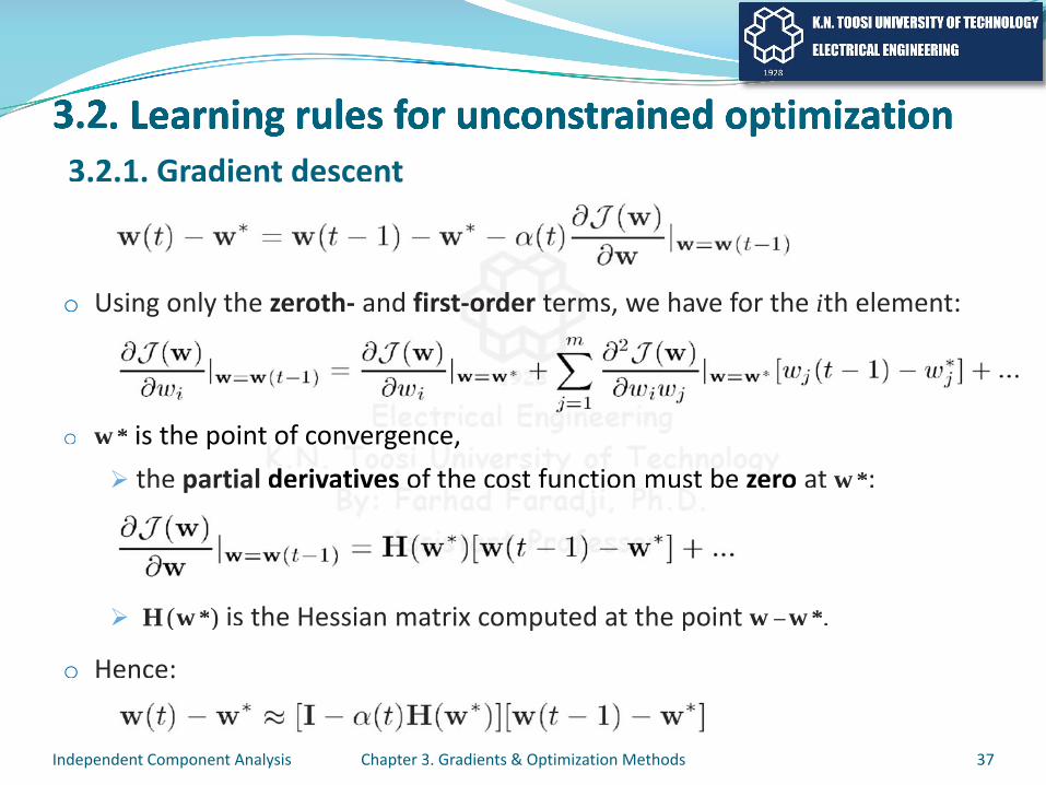
o Using only the zeroth- and first-order terms, we have for the ith element:
o w* is the point of convergence,the partial derivatives of the cost function must be zero at w*:
H(w*) is the Hessian matrix computed at the point w=w*.
o Hence:
Independent Component Analysis Chapter 3. Gradients & Optimization Methods 37
3.2.1. Gradient descent
o Using only the zeroth- and first--oorrdder tteerrmms, we have for the ith element:
o w* is the pointt oooff cccooonnveeerrgencccee,the partial ddderrivaattiivvvess oooof ttthhhe cccoossstt ffuunncccttiiionn mmmuusssstt bbbee zzzeeero at w*:
H(w*) is the Hessian matrix computed at the point w=w*.
o Hence:
Independent Component Analysis Chapter 3. Gradients & Optimization Methods 37
3.2.1. Gradient descent

3.2. Learning rules for unconstrained optimization
o This kind of convergence, which is essentially equivalent to multiplying a matrix many times with itself, is called linear.
o The speed of convergence depends onthe learning rate andthe size of the Hessian matrix.
o If the cost function (w) is very flat at the minimum, with second partial derivatives also small, then
the Hessian is small and the convergence is slow (for fixed (t)).
o Usually, we cannot influence the shape of the cost function.
o We have to choose (t), given a fixed cost function.Independent Component Analysis Chapter 3. Gradients & Optimization Methods 38
3.2.1. Gradient descent
o This kind of convergence, whichh iiss essseennttiially equivalent to multiplying a matrix many times with itself, is ccaalllleedd lliinear.
o The speed of convergencce dependdsss ooonnnnthe learningggg rraatee andddthe size of ttthhhhee HHHeesssssiiann maaatttriiixx..
o If the cost function (w) iissss vvveeeeerryyyyy fflllllaaaattttt aatttt tttthhheeeee mmmmiinnnniiiiimmmmmum, with second partial derivatives also small, then
the Hessian is small and the convergence is slow (for fixed (t)).
o Usually, we yy cannot influence the shape of the cost function.
o We have to choose (t), given a fixed cost function.Independent Component Analysis Chapter 3. Gradients & Optimization Methods 38
3.2.1. Gradient descent
3.2. Learning rules for unconstrained optimization
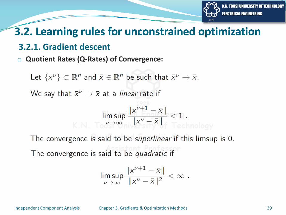
o Quotient Rates (Q-Rates) of Convergence:
Independent Component Analysis Chapter 3. Gradients & Optimization Methods 39
3.2.1. Gradient descento Quotient Rates (Q-Rates) of Convergence:
Independent Component Analysis Chapter 3. Gradients & Optimization Methods 39
3.2.1. Gradient descent
3.2. Learning rules for unconstrained optimization
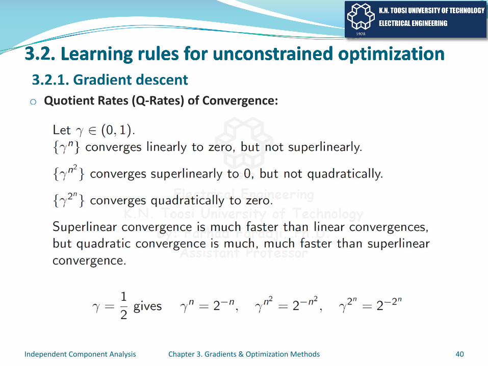
o Quotient Rates (Q-Rates) of Convergence:
Independent Component Analysis Chapter 3. Gradients & Optimization Methods 40
3.2.1. Gradient descento Quotient Rates (Q-Rates) of Convergence:
Independent Component Analysis Chapter 3. Gradients & Optimization Methods 40
3.2.1. Gradient descent

3.2. Learning rules for unconstrained optimization
o The choice of an appropriate step length or learning rate (t) is thus essential.
Too small a value will lead to slow convergence.Too large a value will lead to overshooting and instability,
which prevents convergence altogether.
o Too large a learning rate will cause the solution pointto zigzag around the local minimum.
o The problem is that we do not know the Hessian matrix and thereforedetermining a good value for the learning rate is difficult.
Independent Component Analysis Chapter 3. Gradients & Optimization Methods 41
3.2.1. Gradient descento The choice of an appropriate step length or learning rate (t) is thus
essential.Too small a value will lead too sslloow ccoonnvergence.Too large a value will lead to oovveerrsshhoooting and instability,
which prevents convergencee aaaalllttttooooogether.
o Too large a learrninngggg ratee wiiiilllllll caauuuseee tthhhheee ssssolllllutttiiiionn pppppointto zigzag arounndddd ttthhhhee lllooocccall mmmiiinniimmmuummm.
o The problem is that we dooooo nnnooooott kkkkknnnnnoooowwwww tttthhhhheee HHHHHeeessssssssiiaaaaannnn matrix and thereforedetermining a good value for the learning rate is difficult.
Independent Component Analysis Chapter 3. Gradients & Optimization Methods 41
3.2.1. Gradient descent
3.2. Learning rules for unconstrained optimization
o A simple extension to the basic gradient descent,popular in neural network learning rules
like the back-propagation algorithm,is to use a two-step iteration instead of one-step update rule,
leading to the momentum method.
o Neural network literature has produced a large number of tricks for boosting steepest descent learning by
adjustable learning rates,clever choice of the initial value, etc.
o However, in ICA, many of the most popular algorithms are still straightforward gradient descent methods.
Independent Component Analysis Chapter 3. Gradients & Optimization Methods 42
3.2.1. Gradient descento A simple extension to the basic gradient descent,
popular in neural network leaarrnniinngg rruleslike the back-propagationn aallggoriitthhmm,
is to use a two-step iteration instead off one-step update rule,leading to the momenntum metthhhhhoooddddd.
o Neural networrkkkk liiiitttteeeeraattttuuuuurre hhhaass pppprrrroddduuccceeeeddd a laaaarrgggeeee nnnuuuuumbbbeeeerr ooff tricks for boosting steepesstttt ddddeeessccceeeennnttt llleeeaarrrrnnnniiinnnggggg bbbbyyyyy
adjustable learningggg rraaattttteeeeessss,,,,,clever choice of the initial value, etc.
o However, in ICA, many of the most popular algorithms are still straightforward gradient descent methods.
Independent Component Analysis Chapter 3. Gradients & Optimization Methods 42
3.2.1. Gradient descent
o
oooo
o
o
oooo
o
o (w)w
o (w)
(w)
o (w)w
o ((((wwwww)))
(wwwww)

o
o
o
o
oo
o
o
w
oo
o
o
w

oo

o
oo w*
o
oo w*
oo
o
o
oo
o
o
o
o
o
oI
o
o
o
oI
o
o
oo
o
o
oo
o
o
o
o m m
o
o
o
o
o mmmmmm m
o
oW
W
(W W)
W
oo g
o
oW
W
(W W)
W
oo g
o
o(W)
WWTW
o (W)
o(W)
WWWWWWTWTT
o (W)
o (W W)
oW W W= DW
o M M
o
o (W W)
oW W W= DW
o M MM
o
oo
o
(W) (w)
oo
o
o
o
(W) (w)
oo
o
o
o
x
f(x)
f(x)
o x( ) x( )
o
o
x
f(ff x)
ffffff(((((fffffffff xxxxx))))))
o xxxx((((( )))))) xxxxxx(((( )
o
o
oo
ox( ) x( ) x(T)
o
o
oo
ox(((( ))) xx((( )))) xx(((TTT)))))TTT
o
o
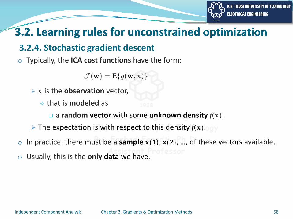
w x
o g(w,x)w
o
w x
o g(w,x)w
o
ox( ) x( )
o
o
ox( ) x( ))
o
o
x(t)
o
o
x(t)
o
o
o
o
o
o
o
o
x(t)
o
Tx(t) t= , , ..., T
T
o
x(t)
o
Tx(t) t= , , ..., T
TTT

o
o
o x(t)
oo
o
o
o xxxx((((tt))))))
oo
o
o
o
o
o x x=As
s
A
o s A
x x
os x
oy=wTx
w
y s
o x x=As
s
A
o sssss AAAAAA
x xx
ossss x
oy=wTxTT
w
y s
oy=wTx
o x( ) x( ) x(T) x
o w
wTx
oy=wTxTT
o xxxx(( )))) xxxxx((((( )) xxxxx(((((TTTTT)))TTTTTT xxxxxx
o w
wwwwwTTTTTTxxxxTTTTTT
o
o w
o(t)
o
o ww
o(t)
ox( ) x( ) x(T)
w
oxx( ) x( ) x(T)TT
w
o
w
w
o
o
wwwwww
w
o

o (w)
w
o
Hi(w), i = , ..., k k w
o (w)
w
o
HiHH (w), i = , ..., k kk w

o
o
k
o
o
k
ow
o (w, , …, k)
i Hi(w)
o (w, , …, k) w
ow
o (w, , …, k)
i HHHHiiiiHH ((wwww))))
o (((((wwwwww,,, ,,,, ……………,,,,, kkkkk))))) w
o
o
(w) (w, , …, k)
o
o
(w)) (w, , …, k)
o
w
w
o
o
w
o
w
w
o
o
w

o x
o
o
o
o
o x
o
o
o
o
o
o w
o
o
o wwww
o

o
w
o
w
o
oo w
wm
oo
o
oo wwwww
wwwwwwm
oo
o
o
o
oo
g(w)
o
o
o
oo
g(w)
o
o
o
o
o
o
o
o
o
o
w
o
o
w