Chapter 3 Hellinger differentiability - Yale Universitypollard/Manuscripts+Notes/Paris2001/Lectures/DQM.pdf · Chapter 3 Hellinger differentiability Modern statistical theory makes

DRAFT: 20 March 2001 David Pollard

Chapter 3

Hellinger differentiability

Modern statistical theory makes clever use of the fact that square roots of probabilitydensity functions correspond to unit vectors in spaces of square integrable functions.The Hellinger distance between densities corresponds to theL2 norm of thedifference between the unit vectors. This Chapter explains some of the statisticalconsequences of differentiability in norm of the square root of the density, a propertyknown as Hellinger differentiability.

SECTION 1 relates Hellinger differentiability to the classical regularity conditions formaximum likelihood theory.

SECTION 2 derives some subtle consequences of norm differentiability for unit vectors.SECTION 3 shows that Hellinger differentiability of marginal densities implies existence of

a local quadratic approximation to the likelihood ratio for product measures.SECTION 4 explains why Hellinger differentiability almost implies contiguity for product

measures.SECTION 5 derives the information inequality, as an illustration of the elegance brought

into statistical theory by Hellinger differentiability.SECTION 6 discusses connections between Hellinger differentiability and pointwise differ-

entiability of densities, leading to a sufficient condition for Hellinger differentiability.SECTION 7 explains how one can dispense with the dominating measure for the definition

of Hellinger differentiability. The slightly strengthened concept—Differentiability inQuadaratic Mean—is shown to be preserved under measurable maps.

Notation: Throughout the Chapter,P := {Pθ : θ ∈ �} will denote a family ofprobability measures, on a fixed(X, A), indexed by a subset� of Rk. In all Sectionsexcept the last,fθ will denote the density ofPθ with respect to a fixed dominatingmeasureλ. The functionξθ (x) will always denote the positive square root offθ (x),and‖ · ‖2 will always denote theL2(λ) norm.

Most results in the Chapter will concern behavior near some arbitrarily chosenpoint θ0 of �. For simplicity of notation, I will usually assumeθ0 = 0, except in afew basic definitions. Thus an expression such as(θ − θ0)

′ξθ0 will simplify to θ ′ξ0,a form that is easier to read and occupies less space on the page. The simplificationinvolves no loss of theoretical generality, because the same effect could always beachieved by a reparametrization,θ := t + θ0.

Pollard@Paris2001 20 March 2001

2 Chapter 3: Hellinger differentiability

1. Heuristics

The traditional regularity conditions for maximum likelihood theory involve existenceof two or three derivatives of density functions, together with domination assumptionsto justify differentiation under integral signs. Le Cam (1970) noted that suchconditions are unnecessarily stringent. He commented:

Even if one is not interested in the maximum economy of assumptions one cannotescape practical statistical problems in which apparently “slight” violations ofthe assumptions occur. For instance the derivatives fail to exist at one pointxwhich may depend onθ , or the distributions may not be mutually absolutelycontinuous or a variety of other difficulties may occur. The existing literatureis rather unclear about what may happen in these circumstances. Note also thatsince the conditions are imposed upon probability densities they may be satisfiedfor one choice of such densities but not for certain other choices.

Probably Le Cam had in mind examples such as the double exponential density,1/2 exp(−|x − θ |), for which differentiability fails at the pointθ = x. He showedthat the traditional conditions can, for some purposes, be replaced by a simplerassumption ofHellinger differentiability: differentiability in norm of the squareroot of the density as an element of anL2 space.

As you will soon see, much asymptotic theory can be made to work withclassical regularity assumptions relaxed to assumptions of Hellinger differentiability.The derivation of the information inequality in Section5 illustrates the point.

<1> Definition. A map τ from a subset� of a Euclidean spaceRk into a normedvector spaceV is said to be differentiable (in norm) at a pointθ0 with derivativeτθ0

if τ(θ) = τ(θ0) + (θ − θ0)′τθ0 + r (θ), where‖r (θ)‖ = o(|θ − θ0|) as θ → θ0. The

derivativeτθ0 is a k-vector (v1, . . . , vk) of elements fromV, and t ′τθ0 = ∑i ti vi .

The family P := {Pθ : θ ∈ �} (dominated byλ) is said to be Hellingerdifferentiability at θ0 if the mapθ �→ ξθ (x) := √

fθ (x) is differentiable inL2(λ)

norm atθ0. That is,P is Hellinger differentiable atθ0 if there exists a vectorξθ0(x)

of functions inL2(λ) such that

<2> ξθ(x) = ξθ0(x) + (θ − θ0)′ξθ0(x) + rθ (x) with ‖rθ‖2 = o(|θ − θ0|) asθ → θ0.

Remark. Some authors (for example, Bickel, Klaassen, Ritov & Wellner (1993,page 202)) adopt a slightly different definition,√

fθ (x) =√

fθ0(x) + 1/2(θ − θ0)′�(x)

√fθ0(x) + rθ (x),

replacing the Hellinger derivativeξθ0 by 1/2�(x)√

fθ0(x). As explained in Section7,the modification very cleverly adds an extra regularity assumption to the definition.The two definitions are not completely equivalent.

Classical statistical theory, especially when dealing with independent observa-tions from aPθ , makes heavy use of the function�θ (x) := log fθ (x). The variancematrix Iθ of the score function(the vector�θ (x) of partial derivatives with respectto θ) is called theFisher information matrix for the model. The classical regularityconditions justify differentiation under the integral sign to get

<3> Pθ �θ (x) = λ fθ (x) = ∂

∂θλ fθ (x) = 0,


3.1 Heuristics 3

whenceIθ := varθ(�θ

) = Pθ

(�θ �

′θ

).

Under assumptions of Hellinger differentiability, the derivativeξθ takes overthe role of the score vector. Ignoring problems related to division by zero anddistinctions between pointwise andL2(λ) differentiability, we would have

2ξθ (x)

ξθ (x)

?= 2√fθ (x)

∂

∂θ

√fθ (x) = 1

fθ (x)

∂ fθ (x)

∂θ= �θ (x).

The equality<3> corresponds to the assertionPθ

(ξθ /ξθ

) = λ(ξθ ξ

) = 0, whichSection2 will show to be a consequence of Hellinger differentiability and theidentity λ fθ ≡ 1. The Fisher informationIθ at θ corresponds to the matrix

Pθ0

(�θ �

′θ

) ?= 4Pθ0

(ξθ ξ

′θ /ξ

2θ

) ?= 4λ(ξθ ξ

′θ

).

Here I flag both equalities as slightly suspect, not just for the unsupported assumptionof equivalence between pointwise and Hellinger differentiabilities, but also becauseof a possible 0/0 cancellation. Perhaps it would be better to insert an explicitindicator function,{ξθ > 0}, as a factor, to protect against 0/0. To avoid possibleambiguity or confusion, I will writeIθ for 4λ(ξθ ξ

′θ ) and I◦

θ for 4λ(ξθ ξ′θ {ξθ > 0}), to

hint at equivalent forms forIθ without yet giving precise conditions under which allthree exist and are equal.

The classical assumptions also justify further interchanges of integrals andderivatives, to derive an alternative representationIθ = −Pθ �θ for the informationmatrix. It might seem obvious that there can be no analog of this representationfor Hellinger differentiability. Indeed, how could an assumption of one-timesdifferentiability, in norm, imply anything about a second derivative? Surprisingly,there is a way, if we think of second derivatives as coefficients of quadratic termsin local approximations. As shown in Section3, the fact that‖ξθ‖2 ≡ 1 leads to aquadratic approximation for a log-likelihood ratio—a sort of Taylor expansion toquadratic terms without the usual assumption of twice continuous differentiability.Remarkable.

2. Differentiability of unit vectors

Supposeτ is a map fromRk into some inner product spaceH (such asL2(λ)).Suppose also thatτ is differentiable (in norm) atθ0,

τθ = τθ0 + (θ − θ0)′τθ0 + rθ with ‖rθ‖ = o(|θ − θ0|) nearθ0.

For simplicity of notation, supposeθ0 = 0.The Cauchy-Schwarz inequality gives|〈τ0, rθ 〉| ≤ ‖τ0‖ ‖rθ‖ = o(|θ |). It would

usually be a blunder to assume naively that the bound must therefore be of orderO(|θ |2); typically, higher-order differentiability assumptions are needed to deriveapproximations with smaller errors. However, if‖τθ‖ is constant—that is, ifτθ

is constrained to take values lying on the surface of a sphere—then the naiveassumption turns out to be no blunder. Indeed, in that case, it is easy to show that ingeneral〈τ0, rθ 〉 equals a quadratic inθ plus an error of ordero(|θ |2). The sequentialform of the assertion will be more convenient for the calculations in Section3.



<4> Lemma. Let {αn} be a sequence of constants tending to zero. Letτ0, τ1, . . . beelements of norm one for whichτn = τ0 + αnW + ρn, with W a fixed element ofHand‖ρn‖ = o(αn). Then〈τ0, W〉 = 0 and2〈τ0, ρn〉 = −α2

n‖W‖2 + o(α2n).la théorème

du chat mortProof. Because bothτn andτ0 have unit length,

0 = ‖τn‖2 − ‖τ0‖2 = 2αn〈τ0, W〉 order O(αn)

+ 2〈τ0, ρn〉 ordero(αn)

+ α2n‖W‖2 order O(α2

n)

+ 2αn〈W, ρn〉 + ‖ρn‖2 ordero(α2n).

The o(αn) ando(α2n) rates of convergence in the second and fourth lines come from

the Cauchy-Schwarz inequality. The exact zero on the left-hand side of the equalityexposes the leading 2αn〈τ0, W〉 as the onlyO(αn) term on the right-hand side. Itmust be of smaller order,o(αn) like the other terms, which can happen only if〈τ0, W〉 = 0, leaving

0 = 2〈τ0, ρn〉 + α2n‖W‖2 + o(α2

n),

as asserted.�Remark. Without the fixed length property, the difference‖τn‖2 − ‖τ0‖2 mightcontain terms of orderαn. The inner product〈τ0, ρn〉, which inheritso(αn) behaviourfrom ‖ρn‖, might then not decrease at theO(α2

n) rate.

<5> Corollary. If P has a Hellinger derivativeξθ0 at 0, and if 0 is an interior pointof �, thenλ

(ξ0ξ0

) = 0 and8λ(ξ0rθ

) = −θ ′I0θ + o(|θ |2) near0.

Proof. Start with the second assertion, in its equivalent form for sequencesθn → 0.Write θn as |θn|un, with un a unit vector inRk. By a subsequencing argument, wemay assume thatun → u, in which case,

ξθn = ξ0 + |θn|u′nξ0 + rθn = ξ0 + |θn|u′ξ0 + (

rθn + |θn|(un − u)′ξ0

).

Invoke the Lemma (withW = u′ξ0) to deduce thatu′λ(ξ0ξ0

) = 0 and

−4|θn|2λ(u′ξ0

)2 + o(|θn|2) = 8λ(ξ0

(rθn + |θn|(un − u)′ξ0

))= 8λ

(ξ0rθn

) + 8|θn|(un − u)′λ(ξ0ξ0

).

Because 0 is an interior point, for every unit vectoru there are sequencesθn → 0through� for which u = θn/|θn|. Thus u′λ

(ξ0ξ0

) = 0 for every unit vectoru,implying that λ

(ξ0ξ0

) = 0. The last displayed equation reduces the sequentialanalog of the asserted approximation.�

Remark. If 0 were not an interior point of the parameter space, there mightnot be enough directionsu along whichθn → 0 through�, and it might not followthat λ(ξ0ξ0) = 0. Roughly speaking, the set of such directions is called thecontingentof � at θ0. If the contingent is ‘rich enough’, we do not need to assume that 0is an interior point. See Le Cam & Yang (1988, Section 6.2) and Le Cam (1986,page 575) for further details. See also the discussion in Section4.


3.3 Quadratic approximation for log likelihood ratios 5

3. Quadratic approximation for log likelihood ratios

Suppose observations{xi } are drawn independently from the distributionP0. Underthe classical regularity conditions, the log of the likelihood ratiod Pn

θ /d Pn0 =∏

i ≤n fθ (xi )/ f0(xi ) has a local quadratic approximation in 1/√

n neighborhoods of 0,underPn

0 . (Remember that, in general,dQ/dP denotes the density with respect toP

of the part ofQ that is absolutely continuous with respect toP.) For example, thefollowing result (for one dimension) was proved in Section2.2.

<6> Theorem. Let Pn := Pn0 and Qn := Pn

θn, for θn := δn/

√n with {δn} bounded.

Suppose the mapθ �→ fθ is twice differentiable in a neighborhoodU of 0 with:

(i) θ �→ fθ (x) is continuous at0;

(ii) there exists aλ-integrable functionM(x) with supθ∈U | fθ (x)| ≤ M(x) a.e. [P0];

(iii) Px0

(fθ (x)/ f0(x)

)2 → Px0

(f0(x)/ f0(x)

)2 =: I0 < ∞ asθ → 0;

(iv) Pθ { f0 = 0} = o(θ2) asθ → 0.

Then P0�0(x) = 0 = P0

(f (x)/ f0(x)

)and, under{Pn},

dQn

dPn= (

1 + op(1))exp

(δnZn − 1

2δ2

nI0),

whereZn := ∑i ≤n �0(xi )/

√n� N(0, I0). Consequently,Qn � Pn.

The method of proof consisted of writing the likelihood ratio as∏i ≤n

(1 + εn(xi )

)whereεn(x) := { f0(x) > 0}( fθn(x) − f0(x)

)/ f0(x) ,

then showing that, underPn,

(a) maxi ≤n |εn(xi )| = op(1),

(b)∑

i ≤n εn(xi ) = δnZn + op(1),

(c)∑

i ≤n εn(xi )2 = δ2

nI0 + op(1).

Result (a) plus the fact that∑

i ≤n εn(xi )2 = Op(1) implied that

<7>∏

i ≤n

(1 + εn(xi )

) = (1 + op(1)

)exp

(∑i ≤n

εn(xi ) − 12εn(xi )

2)

,

from which the final assertion followed.Le Cam (1970) established a similar quadratic approximation under an

assumption of Hellinger differentiability. The method of proof is very similar tothe method just outlined, but with a few very subtle differences. Remember thatI0 := 4λ

(ξθ ξ

′θ

)and I◦

0 := 4λ(ξ0ξ

′0{ξθ > 0}).

<8> Theorem. SupposeP is Hellinger differentiable at0, with L2(λ) derivative ξ0.Let Pn := Pn

0 andQn := Pnθn

, with θn := δn/√

n for a bounded sequence{δn}. Then,under{Pn},

dQn

dPn= (

1 + op(1))exp

(δ′

nZn − 14δ′

n(I0 + I◦0)δn

),

whereZn := 2n−1/2

∑i ≤n

{ξ0(xi ) > 0}ξ0(xi )/ξ0(xi )� N(0, I◦0).



Remark. It is traditional to absorb the 1+ op(1) factor for the likelihood ratiointo the exponent. One then has some awkwardness with the right-hand side of theapproximation at samples for which the left-hand side is zero. The awkwardnessoccurs with positivePn probability if Pθ0{ fθn = 0} > 0.

Proof. I will give the proof only for the one-dimensional case. The proof for themulti-dimensional case is analogous.

Write τn for ξθn , andρn for rθn , and Ln for dQn/dPn. By Hellinger differentia-bility,

τn(x) = ξ0(x) + n−1/2δnξ0(x) + ρn(x) with λρ2n = o(θ2

n ).

Define

<9> ηn(x) := {ξ0(x) > 0}τn(x) − ξ0(x)

ξ0(x)= δn√

nD(x) + Rn(x),

where

D(x) := {ξ0(x) > 0}ξ0(x)/ξ0(x) and Rn(x) := {ξ0(x) > 0}ρn(x)/ξ0(x).

The indicator functions have no effect within the setAn := ∩i ≤n{ξ0(xi ) > 0}, which

has Pn-probability one, but they will protect against 0/0 ?= 1 when convertingfrom P0- to λ-integrals. On the setAn ,√

Ln =∏

i ≤nτn(xi )/ξ0(xi ) =

∏i ≤n

(1 + ηn(xi )

).

For almost the same reason as in the proof of Theorem<6>, we need to show that

(i) maxi ≤n |ηn(xi )| = op(1),

(ii)∑

i ≤n ηn(xi ) = 12δnZn − 1

8δ2

n I0 + op(1),

(iii)∑

i ≤n ηn(xi )2 = 1

4δ2

n I◦0 + op(1).

The analog of<7>, with ηn replacingεn, will then give√Ln = (

1 + op(1))exp

(∑i ≤n

ηn(xi ) − 12

∑i ≤n

ηn(xi )2)

,

from which the assertion of the Theorem follows by squaring both sides.

Remark. Notice that (ii) differs significantly from its analog (b) for the proofof Theorem<6>, through the addition of a constant term. However, the differenceis compensated by a halving of the corresponding constant in (iii), as comparedwith (c). The differences occur because, on the set{ f0(x) > 0},

εn(x) = τn(x)2 − ξ0(x)2

ξ0(x)2= τn(x) − ξ0(x)

ξ0(x)

2ξ0(x) + τn(x) − ξ0(x)

ξ0(x)= 2ηn(x) + ηn(x)2.

Thus∑i ≤n

εn(xi ) = 2∑

i ≤nηn(xi ) +

∑i ≤n

ηn(xi )2 = δn Zn − 1

4δ2nI0 + 1

4 I◦0 + op(1).

As you will see in Section4, the conditions of Theorem<6> actually imply I0 = I◦0,

a condition equivalent to the contiguityQn � Pn.

Assertions (i), (ii), and (iii) will follow from<9>, via simple probability facts,including: if Y1, Y2, . . . are independent, identically distributed random variableswith P|Y1|r < ∞ for some constantr ≥ 1 then maxi ≤n |Yi | = op(n1/r ). (The proofappeared as a Problem to Chapter 2.)


3.3 Quadratic approximation for log likelihood ratios 7

First note that

P0D(x) = λ

(ξ0(x)2

ξ0(x)

ξ0(x){ξ0(x) > 0}

)= λ

(ξ0ξ0

) = 0 by Corollary<5>,

P0D(x)2 = λ

(ξ0(x)2

ξ0(x)2

ξ0(x)2{ξ0(x) > 0}

)= λ

(ξ20 {ξ0(x) > 0}) = 1

4I◦0,

8P0R(x) = 8λ (ξ0(x)ρn(x)) = −δ2n I0/n + o(1/n),

P0R(x)2 ≤ λρn(x)2 = o(1/n).

From the expressions involvingD we get

Zn = 2∑

i ≤nD(xi )/

√n� N(0, 1

4I◦),

n−1∑

i ≤nD(xi )

2 = 14I◦ + op(1),

maxi ≤n

|D(xi )| = op(n1/2).

From the expressions involvingRn we get

Pn

(∑i ≤n

Rn(xi ))

= −δ2n I0 + o(1),

var(∑

i ≤nRn(xi )

)≤

∑i ≤n

Pn Rn(xi )2 → 0,

which together imply that∑i ≤n

R(xi ) = − 18δ2

n I0 + op(1),

(maxi ≤n |Rn(xi )|

)2 ≤∑

i ≤nRn(xi )

2 = op(1).

Assertions (i), (ii), and (iii) now follow easily.For (i):

maxi ≤n |ηn(xi )| ≤ |δn| maxi ≤n|D(xi )|√

n+ maxi ≤n |Rn(xi )| = op(1).

For (ii):∑

i ≤nηn(xi ) = 1

2δn

∑i ≤n

D(xi )√n

+∑

i ≤nRn(xi ) = 1

2δnZn − 1

8δ2

n I0 + op(1).

For (iii):∣∣∣(∑

i ≤nηn(xi )

2)1/2

−(

δ2n

∑i ≤n

D(xi )2

n

)1/2∣∣∣ ≤(∑

i ≤nRn(xi )

2)1/2

= op(1),

implying that∑

i ≤nηn(xi )

2 = δ2n

∑i ≤n

D(xi )2

n+ op(1) = 1

4δ2

n I◦0 + op(1).

The asserted quadratic approximation follows.�

4. Contiguity

Consider once more the product measuresPn := Pn0 and Qn := Pn

θn, as defined in

Theorem<8>, under the assumption of Hellinger differentiability atθ = 0. For



contiguity we needPL = 1 for every limit in distribution of a subsequence ofLn := dQn/dPn. Along a further subsequenceδn → δ ∈ Rk, so we must haveL ofthe form

exp(δ′Z − 1

4δ′

(I0 + I◦

0

)δ)

with Z distributedN(0, I◦0).

This random variable has expected value equal to 1 if and only if

δ′I0δ = 12δ′

(I0 + I◦

0

)δ,

which rearranges to the condition

λ((δ′ξ0)

2{ξ0 = 0}) = 0

or, equivalently(δ′ξ0){ξ0 = 0} = 0 a.e. [λ].We also have a necessary condition for contiguity, from Section2.2, namely,

nPθn{ f0 = 0} = o(1/n). With Hellinger differentiability, we have another way toexpress this condition. Ifθn := δn/

√n then ξθn(x) = n−1/2δnξ0(x) + rθn(x) when

ξ(x) = 0, so that

nPθn{ f0 = 0} = nλ(ξ2θn

{ξ0 = 0}) = δ′nλ

(ξ0ξ

′0{ξ0 = 0}) δn + o(1).

If δn → δ, the necessary condition for contiguity becomesδ′ξ0{ξ0 = 0} = 0 a.e. [λ].Putting the two arguments together we get a neater form of Theorem<8>.

<10> Corollary. If P is Hellinger differentiable at0, and if θn = δn/√

n, with {δn}bounded, thenPn

θn� Pn

0 if and only if nPθn{ f0 = 0} → 0. In that case,

d Pnθn

/d Pn0 = (

1 + op(1; Pn))exp

(δ′

nZn − 12δ′

nI0δn

).

Hellinger differentiability alone does not imply contiguity, as shown by asimple counterexample.

<11> Example. DefineP := {Pθ : 0 ≤ θ ≤ 1} via the densities

fθ (x) = ξθ (x)2 := (1 − θ2) (1 − |x|)+ + θ2 (1 − |x − 2|)+

with respect to Lebesgue measureλ on [−1, 3], The densitiesf0 and f1 have disjointsupport, andξθ = (

1 − θ2)1/2

ξ0 + θξ1. By direct calculation

λ |ξθ (x) − ξ0(x) − θξ1(x)|2 =(√

1 − θ2 − 1)2

= O(θ4).

Thus P is Hellinger differentiable atθ = 0 with L2(λ) derivative ξ0 := √f1, but

Pθ { f0 = 0} = θ2. The random variableZn is equal to zero a.e. [Pn0 ], and I0 = 1,

and I0 = 0. What happens to the likelihhood ratio whenθ = δ/√

n?�You might suspect that the extreme behavior in the previous Example is caused

by the fact that the parameter value 0 lies on the boundary of�. That suspicionwould be well founded. At interior points the nonnegativity of the density forcesthe L2(λ) to behave well, leading to a sistuation where Corollary<10> applies.

<12> Corollary. Let P be Hellinger differentiable at0, with L2(λ) derivative ξ0. If0 ∈ int(�), then ξ0{ξ0 = 0} = 0 a.e. [λ], which implies thatPθn{ f0 = 0} = o(1/n) ifθn := δn/

√n, with {δn} bounded.


3.4 Contiguity 9

Proof. Let u be a unit vector inRk. Considerθn := αnu, with αn decreasing to zeroso fast that

∑n ‖rθn‖2/αn < ∞, which impliesrθn(x)/αn → 0 a.e. [λ]. We can then

draw the pointwise conclusionu′ξ (x){ξ0(x) = 0} ≥ 0 a.e. [λ] from the inequality

0 ≤ α−1n ξθn(x){ξ0(x) = 0} = u′ξ (x){ξ0(x) = 0} + rθn(x)/αn a.e. [λ].

The conclusion holds for every unit vector. The assertion of the Corollary follows.�

5. Information inequality

The information inequality for the modelP := {Pθ : θ ∈ �} bounds the variance ofan estimatorT(x) from below by an expression involving the expected value of thestatistic and the Fisher information: under suitable regularity conditions,

varθ (T) ≥ γ ′θ I

−1θ γθ whereγθ := Pθ T(x).

The classical proof of the inequality imposes assumptions that derivatives canbe passed inside integral signs, typically justified by more primitive assumptionsinvolving pointwise differentiability of densities and domination assumptions abouttheir derivatives.

By contrast, the proof of the information inequality based on an assumption ofHellinger differentiability replaces the classical requirements by simple properties ofL2(λ) norms and inner products. The gain in elegance and economy of assumptionsillustrates the typical benefits of working with Hellinger differentiability. The maintechnical ideas are captured by the following Lemma. Once again, with no loss ofgenerality I consider only behavior atθ = 0.

Remark. The measurePθ might itself be a product measure, representing thejoint distribution of a sample of independent observations from some distributionµθ .As shown by Problem[4], Hellinger differentiability ofθ �→ µθ at θ = 0 would thenimply Hellinger differentiability ofθ �→ Pθ at θ = 0. We could substitute an explicitproduct measure forPθ in the next Lemma, but there would be no advantage todoing so.

<13> Lemma. SupposeP is Hellinger differentiable at0 with L2(λ) derivative ξ0.Supposesupθ∈U Pθ T(x)2 < ∞, for some neighborhoodU of 0. Then the expectedvalue,γθ := Px

θ T(x), has derivativeγ0 = 2λ(ξ0ξ0T) at 0.

Remark. Notice that Pθ T is well defined throughoutU , because of the bound

on the second moment. Also(λ|ξ0ξ0T |)2 ≤ (

λξ20 T2

) (λ|ξ0|2

)< ∞.

Proof. Write C2 for supθ∈U Pθ T(x)2, so that‖ξθ T‖2 ≤ C for eachθ in U . Forsimplicity, I consider only the one-dimensional case. The proof forRk differs onlynotationally.



The proof is easy ifT is bounded by a finite constantK .

|γθ − γ0 − 2θλ(ξ0ξ0T)|= |λ (

ξ2θ − ξ2

0 − 2θξ0ξ0

)T |

= λ∣∣θ2ξ2

0 + r 2θ + 2ξ0rθ + 2θ ξ0rθ

∣∣ |T |<14>

≤ K θ2‖ξ0‖22 + K‖rθ‖2

2

+ 2K(‖ξ0‖2 ‖rθ‖2 + |θ |‖ξ0‖2 ‖rθ‖2

)by Cauchy-Schwarz

= o(|θ |).Notice thatK need not be fixed for the last conclusion. It would suffice if we

had|T | ≤ Kθ = o(1/|θ |), which suggests a truncation argument to handle the case ofunboundedT . Let Kθ increase to∞ asθ → 0, in such a way that|θ |Kθ → 0. Thecontributions to the remainder fromT{|T | ≤ Kθ } are of ordero(|θ |). To completethe proof we have only to show that

<15> λ(ξ2θ − ξ2

0 )T{|T | > Kθ } − 2θλ(ξ0ξ0T{|T | > Kθ }

) = o(|θ |).On the left-hand side, the coefficient of 2θ in the second term is bounded in absolutevalue by

λ|ξ0ξ0T{|T | > Kθ }| ≤ ‖ξ0{|T | > Kθ }‖2 ‖ξ0T‖2 ≤ o(1)C,

the o(1) term on the right-hand side coming via Dominated Convergence and theλ-integrability of ξ2

0 . For the first term on the left-hand side of<15>, factorizeξ2θ − ξ2

0 as (θ ξ0 + rθ )(ξθ + ξ0) then expand, to get

|λ(ξ2θ − ξ2

0 )T{|T | > Kθ }|≤ λ|θ ξ0{|T | > Kθ } + rθ | |ξθ T + ξ0T |≤ (|θ | · ‖ξ0{|T | > Kθ }‖2 + ‖rθ‖2

)(‖ξθ T‖2 + ‖ξ0T‖2

),

the last bound following from several applications of the Cauchy-Schwarz inequality.Both terms in the leading factor are of ordero(|θ |); both terms in the other factorare bounded byC. The contribution to the remainder is of ordero(|θ |), as requiredfor differentiability.�

Remember from Section1 that 4λ(ξ0ξ′0) corresponds to the Fisher information

matrix I0.

<16> Corollary. In addition to the conditions of the Lemma, supposeI0 is nonsingular.Thenvarθ0T ≥ γ0I−1

0 γ0.

Proof. The special case whereT ≡ 1 givesλ(ξ0ξ0) = 0 (or use Lemma<4>). Letinterior point?

α be a fixed vector inRk. From Lemma<13> deduce that

(α′γ0)2 = 4

(λ

(α′ξ0

)(T − γ0)ξ0

)2≤ 4α′λ(ξ0ξ

′0)α λ

(ξ20 (T − γ0)

2)

by Cauchy-Schwarz

= α′I0αPθ0 (T − γ0)2

Chooseα := I−10 γ0 to complete the proof.�

Variations on the information inequality lead to other useful lower bounds forvariances and mean squared errors of statistics.


3.5 Information inequality 11

<17> Example. Van Trees inequality—needs to be reworked....

The information inequality for the one-parameter family takes an elegant form,

mθq(θ)Pθ (T(x) − θ)2 ≥ 1Iq + mθq(θ)I(θ)

,

whereIq = 4µη2 = µq2/q denotes the information function for the shift family, andI(θ) = λ�2

θ denotes the information function for theP model.The inequality is known as thevan Trees inequality. It has many statistical

applications. See Gill & Levit (1995) for details.�

6. A sufficient condition for Hellinger differentiability

How does Hellinger differentiability relate to the classical assumption of pointwisedifferentiability?

Consider the case where� is one-dimensional, withθ as an interior point.SupposeP is hellinger differentiable at 0, withL2(λ) derivativeξ0. That is,

ξθ (x) = ξ0(x) + θ ξ0(x) + rθ (x) with ‖rθ‖2 = o(|θ |).If a sequence{θn} tends to zero fast enough, then

∑n ‖rθn‖2/|θn| < ∞, from which it

follows that |rθn(x)| = o(|θn|) a.e. [λ]. Unfortunately the aberrant negligible set ofxmight depend on{θn}, so we cannot immediately invoke the usual subsequencingargument to deduce that|rθ (x)| = o(|θ |) a.e. [λ]. That is, it does not followimmediately thatθ �→ ξθ (x) is differentiable atθ = 0 for λ-almost allx. However,if by some means we can show that the pointwise derivativeξ ′

0(x) does exist thenwe must haveξ(x) = ξ ′

0(x) a.e. [λ].For example, ifθ �→ fθ (x) has derivativef ′

0(x) at θ = 0, and if fθ (x) > 0, then2ξ ′

0(x) = f ′0(x)/ξ0(x). At pointsx where f0(x) = 0, both derivativesf ′

0(x) andξ ′0(x),

if they exist, must be zero, for otherwisefθ (x) or ξθ (x) would be strictly negativefor some smallθ , either positive or negative. Thus, if the pointwise derivativesexists then1

2f ′0(x){ξ0(x) > 0}/ξ0(x) is, up to aλ-equivalence, the only candidate for

a Hellinger derivative atθ = 0.Now consider the situation where we have pointwise differentiability, and

we wish to deduce Hellinger differentiability. What more is needed? The answerrequires careful attention to the problem of when functions of a real variable can berecovered as integrals of their derivatives.

<18> Definition. A real valued functionH defined on an interval[a, b] of the realline is said to beabsolutely continuousif to eachε > 0 there exists aδ > 0 suchthat

∑i |H(bi ) − H(ai )| < ε for all finite collections of nonoverlapping subintervals

[ai , bi ] of [a, b] for which∑

i (bi − ai ) < δ.Absolute continuity of a function defined on the whole real line is taken to

mean absolute continuity on each finite subinterval.

The following connection between absolute continuity and integration ofderivatives is one of the most celebrated results of classical analysis (UGMTP §3.4).



<19> Theorem. A real valued functionH defined on an interval[a, b] is absolutelycontinuous if and only if the following three conditions hold.

(i) The derivativeH ′(t) exists at Lebesgue almost all points of[a, b].

(ii) The derivativeH ′ is Lebesgue integrable

(iii) H(t) − H(a) = ∫ ta H ′(s) ds for eacht in [a, b]

Put another way, a functionH is absolutely continuous on an interval [a, b] ifand only if there exists an integrable functionh for which

<20> H(t) =∫ t

ah(s) ds for all t in [a, b]

The function H must then have derivativeh(t) at almost allt . As a systematicconvention we could takeh equal to the measurable function

H(t) ={

H ′(t) at pointst where the derivative exists,0 elsewhere.

I will refer to H as thedensity. Of course it is actually immaterial howH is definedon the Lebesgue negligible set of points at which the derivative does not exist, butthe convention helps to avoid ambiguity.

Now consider anonnegativefunction H that is differentiable at a pointt . IfH(t) > 0 then the chain rule of elementary calculus implies that the function 2

√H

is also differentiable att , with derivativeH ′(t)/√

H(t). At points whereH(t) = 0,the question of differentiability becomes more delicate, because the mapy �→ √

y isnot differentiable at the origin. Ift is an internal point of the interval andH(t) = 0then we must haveH ′(t) = 0. ThusH(y) = o(|y− t |) neart . If

√H had a derivative

at t then√

H(y) = o(|y − t |) neart , and henceH(y) = o(|y − t |2). Clearly we needto take some care with the question of differentiability at points whereH equalszero.

Even more delicate is the fact that absolute continuity of a nonnegativefunction H need not imply absolute continuity of the function

√H , without further

assumptions—even ifH is everywhere differentiable (Problem[1]).

<21> Lemma. Suppose a nonnegative functionH is absolutely continuous on aninterval [a, b], with density H . Let �(t) := 1/2H(t){H(t) > 0}/√H(t). If∫ b

a |�(t)| dx < ∞ then√

H is absolutely continuous, with density�, that is,

√H(t) −

√H(a) =

∫ t

a�(s) ds for all t in [a, b]

Proof. Fix an η > 0. The functionHη := η + H is bounded away from zero,and hence

√Hη has derivativeH ′

η = H ′/(2√

H + η) at each point where thederivativeH ′ exists. Moreover, absolute continuity ofHη follows directly from theDefinition <18>, because

|√Hη(bi ) − √Hη(ai )| = |Hη(bi ) − Hη(ai )|√

Hη(bi ) + √Hη(ai )

≤ |H(bi ) − H(ai )|2√

η

for each interval [ai , bi ]. From Theorem<19>, for eacht in [a, b],√

H(t) + η −√

H(a) + η =∫ t

a

H(s)

2√

H(s) + ηds.


3.6 A sufficient condition for Hellinger differentiability 13

As η decreases to zero, the left-hand side converges to√

H(t) − √H(a). The

integrand on the right-hand side converges to�(s) at points whereH(s) > 0. Foralmost alls in {H = 0} the derivativeH ′(s) exists and equals zero; the integrandconverges to 0= �(s) at those points. By Dominated Convergence, the right-handside converges to

∫ ta �(s) ds.�

The integral representation for the square root of an absolutely continuousfunction is often the key to proofs of Hellinger differentiability.

<22> Theorem. SupposeP = {Pθ (x) : |θ | < δ} for someδ > 0, with eachPθ dominatedby a sigma-finite measureλ. Suppose also that

(i) there exist densities such that(x, θ) �→ fθ (x) is product measurable;

(ii) for λ almost allx, the functionθ �→ fθ (x) is absolutely continuous on[−δ, δ],with density fθ (x);

(iii) for λ almost allx, the functionθ �→ fθ (x) is differentiable atθ = 0;

(iv) for eachθ the function�θ(x) := 12

fθ (x){ fθ (x) > 0}/√ fθ (x) belongs toL2(λ)

andλ�2θ → λ�2

0 asθ → 0.

ThenP has Hellinger derivative�0(x) at θ = 0.

Remark. Assumption (iii) might appear redundant, because (ii) impliesdifferentiability of θ �→ fθ (x) at Lebesgue almost allθ , for λ-almost all x. Amathematical optimist (or Bayesian) might be prepared to gamble that 0 doesnot belong to the bad negligible set; a mathematical pessimist might preferAssumption (iii).

Proof. As before writeξθ (x) for√

fθ (x), and definerθ (x) := ξθ (x)−ξ0(x)−θ�0(x).We need to prove thatλr 2

θ = o(|θ |2) asθ → 0.For simplicity of notation, consider only positiveθ . The arguments for

negativeθ are analogous. Writem for Lebesgue measure on [−δ, δ]With no loss of generality (or by a suitable decrease inδ) we may assume that

λ�2θ is bounded, so that, by Tonelli,∞ > msλx�s(x)2 = λxms�s(x)2, implying

ms�s(x)2 < ∞ a.e. [λ]. From Lemma<21> it then follows that

ξθ (x) − ξ0(x)

θ= 1

θ

∫ θ

0

�s(x) ds a.e. [λ].

By Jensen’s inequality for the uniform distribution on [0, θ ], and (iv),

<23> λ

∣∣∣∣ξθ (x) − ξ0(x)

θ

∣∣∣∣2

≤ 1θ

∫ θ

0

λ�s(x)2 ds → λ�20 asθ → 0.

Define nonnegative, measurable functions

gθ (x) := 2 |ξθ (x) − ξ0(x)|2 /θ2 + 2�0(x)2 − |rθ (x)/θ |2 .

By (iii), rθ (x)/θ → 0 at almost allx whereξ0(x) > 0, and hencegθ (x) → 4�0(x)2;and�0(x) = 0 whenξ0(x) = 0. Thus lim infgθ (x) ≥ 4�0(x)2 a.e. [λ]. By Fatou’sLemma (applied along subsequences), followed by an appeal to<23>,

4λ�20 ≤ lim inf

θ→0λgθ ≤ 4λ�2

0 − lim supθ→0

λ |rθ (x)/θ |2 .

That is,λr 2θ = o(θ2), as required for Hellinger differentiability.�



<24> Example. Let f be a probability density with respect to Lebesgue measureλ

on the real line. Supposef is absolutely continuous, with densityf for whichI := λ

({ f > 0} f 2/ f)

< ∞. Define Pθ to have densityfθ (x) := f (x − θ) withrespect toλ, for eachθ in R. The conditions of Theorem<22> are satisfied, withλ�2

θ ≡ I. The family {Pθ : θ ∈ R} is Hellinger differentiable atθ = 0. In fact, thesame argument works at everyθ ; the family is everywhere Hellinger differentiable.�

7. An intrinsic characterization of Hellinger differentiability

For the definition of Hellinger differentiability, the choice of dominating measureλ

for the family of probability measuresP = {Pθ : θ ∈ �} is somewhat arbitrary. Infact, there is really no need for a single dominatingλ, provided we guard againstcontributions fromP⊥

θ , the part ofPθ that is singular with respect toP0. As yousaw in Section4, the assumptionP⊥

θ X = o(|θ |2) is needed to ensure contiguity.We lose little by building the assumption into the definition. Following Le Cam &Yang (2000, Section 7.2), I will call the slightly stronger propertydifferentiabilityin quadratic mean (DQM), to stress that the definition requires a little more thanHellinger differentiability.

The definition makes no assumption that the family of probability measuresP := {Pθ : θ ∈ �} is dominated. Instead it is expressed directly in terms of theLebesgue decomposition ofPθ with respect toPθ0, for a fixedθ0 in �. As before, Iwill assumeθ0 = 0 to simplify notation. Remember thatPθ = Pθ + P⊥

θ , where theabsolutely continuous partPθ has a densitypθ with respect toP0 and the singularpart P⊥

θ concentrates on aP0-negligible setNθ ,

Pθ g = Pθ

(g(x)pθ (x){x ∈ Nc

θ }) + P⊥

θ

(g(x){x ∈ Nθ }

),

at least for nonnegative measurable functionsg on X.

<25> Definition. Say thatP is differentiability in quadratic mean (DQM) at0 if

(i) P⊥θ (X) = o(|θ |2) as |θ | → 0,

(ii) there is a vector� of k functions fromL2(P0) for which√pθ (x) = 1 + 1

2θ ′�(x) + rθ (x) with P0

(r 2θ

) = o(|θ |2) near 0.

Remark. Some authors (for example, Bickel et al. 1993, page 457) use the termDQM as a synonym for differentiability inL2 norm. The factor of 1/2 simplifiessome calculations, by making the vector� correspond to thescore functionat 0.

WhenP is dominated by a sigma-finite measure, the definition agrees with thedefinition of Hellinger differentiability under the assumption (i), which is neededfor contiguity of product measures.

<26> Theorem. SupposeP is dominated by a sigma-finite measureλ, with correspond-ing densitiesfθ (x).

(i) SupposePθ { f0 = 0} = o(|θ |2) and, for some vectorξ of functions inL2(λ),√fθ (x) =

√f0 + θ ′ξ (x) + Rθ (x) whereλ

(R2

θ

) = o(|θ |2) with θ = 0.


3.7 An intrinsic characterization of Hellinger differentiability 15

ThenP satisfies the DQM condition at0, with � := 2{ f0 > 0}ξ /√

f0 andrθ := { f0 > 0}Rθ /

√f0.

(ii) If P satisfies the DQM condition at0 then it is also Hellinger differentiableat 0, with L2(λ) derivativeξ := 1

2�

√f0.

Proof. For the Lebesgue decomposition we can takepθ := { f0 > 0} fθ / f0 andNθ := { f0 = 0}. Thus P⊥

θ X = λ fθ { f0 = 0}.If P is Hellinger differentiability, as in (i), the

P0

∣∣√pθ − 1 − 12θ ′�

∣∣2 = λ f0∣∣∣{ f0 > 0}

√fθ / f0 − 1 − 1

2θ ′ξ{ f0 > 0}/

√f0

∣∣∣2

= λ

({ f0 > 0}

∣∣∣√ fθ −√

f0 − θ ′ξ∣∣∣2

)= o(|θ |2).

Conversely, ifP satisfies DQM then

λ

∣∣∣√ fθ −√

f0 − θ ′ξ∣∣∣2 = λ{ f0 = 0}

(√fθ − 0

)2

+ λ{ f0 > 0}∣∣∣√ f0 pθ −

√f0 − 1

2θ ′�

√f0

∣∣∣2= o(|θ |2) + P0

∣∣√pθ − 1 − 12θ ′�

∣∣2 = o(|θ |2).�

Remark. The proof of the previous Theorem is almost trivial, once onerealizes that contributions from{ f0 = 0} need separate consideration. Both� and ξ

vanish on that set. For the definition of Hellinger differentiability it is not, a priori,necessary thatξ{ f0 = 0} = 0. Indeed, it is contributions from that term that canupset contiguity. Some authorsdefineHellinger differentiability atθ = 0 to mean

λ|√

fθ −√

f0 − 12θ ′�

√f0|2 = o(|θ |2) with P0|�|2 < ∞,

thereby forcing theL2(λ) derivative to vanish on{ f0 = 0}. In effect, such a definitionmakes contiguity for the product measures a requirement of differentiability in theL2(λ) sense.

The definition of DQM has some advantages over the definition of Hellingerdifferentiability, even beyond the elimination of the dominating measureλ. For θ

near zero,pθ ≈ 1, a simplification that has subtle consequences, as illustrated bythe next Theorem.

The result concerns preservation of the DQM property under measurable maps.Specifically, if T is a measurable map from(X, A) to (Y, B)) then eachPθ inducesan image measureQθ := T(Pθ ) on B, defined byQθ g := Px

θ g(T x) for eachg inM+(Y, B). For eachh in M+(X, A) we can also define a measureνh on B by

νh(g) := Px0 (h(x)g(T x)) for eachg in M+(Y, B).

The measureνh is absolutely continuous with respect toQ0, because ifQ0g = 0,for a g in M+(Y, B), theng(T x) = 0 a.e. [P]. I will denote the densitydνh/d Q0 byπt (h). That is,

<27> Px0

(h(x)g(T x)

) = Qt0 (g(t)πt (h)) for eachg ∈ M+(Y, B), andh ∈ M+(X, A).

In fact, πt (h) is the Kolmogorov conditional expectation, usually denoted byP0(h | T = t). (Compare withUGMTP §5.6.)



As a particular case, the image measureT(Pθ ) is absolutely continuous withrespect toQ0, with densityP0(pθ | T = t) = πt (pθ ). Under DQM,

√πt (pθ ) =

(πt

(1 + 1

2θ ′� + rθ

)2)1/2

= (1 + θ ′πt� + . . .

)1/2 = 1 + 12θ ′πt� + . . .

If all the omitted terms can be ignored, in anL2(Q0) sense, then{T Pθ : θ ∈ �}would be Hellinger differentiable at 0, withL2(Q0)-derivativeπt (�). The imageof the singular parts,T(P⊥

θ ), has total masso(θ |2), which does not disturb theapproximation.

<28> Theorem. SupposeP = {Pθ : θ ∈ �} is DQM at 0 with score function�.SupposeT is a measurable map from(X, A) into (Y, B). Then {T Pθ : θ ∈ �} isDQM at 0, with score functionP0(� | T = t).

Proof. To simplify notation, I will assume� is one-dimensional. No extraconceptual difficulties arise in higher dimensions.

Define Qθ := T Pθ and Qθ := T Pθ . Write ξθ for√

pθ , so that

ξθ (x) = 1 + 12θ�(x) + rθ (x) with P0r 2

θ = o(θ2).

Use a bar to denote “averaging” with respect toπt ,

�θ (t) := πt (�), rθ (t) := πt (rθ ), ξθ (t) := πt (ξθ ) = 1 + 12θ�(t) + rθ (t).

Define conditional variances similarly,

σ 2θ (t) := πt

(ξθ − ξθ

)2, J(t) := πt

(� − �

)2, εθ (t)

2 := πt (rθ − rθ )2 .

Notice thatQ0σ

2θ ≤ Q0

(πtξ

2θ

) = P0ξ2θ = PθX ≤ 1,

andQ0 J ≤ Q0

(πt�

2) = P0�

2 < ∞,

andQ0ε

2θ ≤ Q0

(πt r

2θ

) = P0r 2θ = o(θ2).

The density ofQθ with respect toQ0 equals

η2θ (t) := πt (ξ

2θ ) = πt (ξθ − ξθ )

2 + ξ2θ .

Thusδθ (t) := ηθ (t) − ξθ (t) is nonnegative, and(ξθ + δθ

)2 = η2θ = σ 2

θ + ξ2θ , implying

<29> 2ξθ δθ + δ2θ = σ 2

θ = πt(12θ(� − �) + (rθ − rθ )

)2 ≤ 12θ2 J(t) + 2ε2

θ (t).

Remark. The cancellation of the leading constants whenξθ is subtractedfrom ξθ seems to be vital to the proof. For general Hellinger differentiability, thecancellation does not occur.

DQM for the Qθ measures meansQ0

(ηθ − 1 − 1

2θ�

)2 = o(θ2). The differenceηθ − 1 − 1

2θ� equalsδδ + rθ . The rθ is easily handled:

Q0r 2θ = Q0 (πt rθ )

2 ≤ Q0πt r2θ = P0r 2

θ = o(θ2).


3.7 An intrinsic characterization of Hellinger differentiability 17

For δθ we need to argue from<29>, using the fact thatξθ should be close to 1.More precisely, letMθ be a positive constant (depending onθ) for which Mθ → ∞and 1/2 ≥ |θ |Mθ → 0 asθ → 0. Then the set

�θ := {t : J(t) ≤ Mθ , |�(t)| ≤ Mθ , |rθ | ≤ 14, |εθ | ≤ 1},

hasQ0 measure tending to 1, and on�θ ,

ξθ (t) ≥ 1 − 12|θ�(t)| − |rθ (t)| ≥ 1

2.

Splitting the integrand according to whethert is in �θ or not, and reducing theleft-hand side of<29> to 2ξθ δθ ≥ δθ in the first case andδ2

θ in the second, we have

Q0δ2θ ≤ Q0

((12θ2 J(t) + 2ε2

θ (t))2 {t ∈ �θ }

)+ Q0

(12θ2 J(t) + 2ε2

θ (t){t ∈ �cθ }

)≤ 2

(12θ2Mθ

)2 + 12θ2Q0 (J(t){J(t) > Mθ }) + 6Q0ε

2θ

= o(θ2).

Dominated Convergence takes care of the middle term.The part ofQθ that is absolutely continuous with respect toQ0 might be slightly

larger thanQθ , because the image measureT P⊥θ might also make a contribution.

That is, the density for the Lebesgue decomposition ofQθ with respect toQ0 mightactually equalη2

θ + sθ , wheresθ ≥ 0 andQ0sθ ≤ (T P⊥θ )(Y) = P⊥

θ (X) = o(θ2).The contribution fromsθ gets absorbed into the remainder term, and adds furthero(θ2) terms to the bounds in the previous paragraph. The modification has anasymptotically negligible effect on the argument. The family{Qθ : θ ∈ �} inheritsDQM from the family {Qθ : θ ∈ �}.�

8. Problems

Problems not yet checked.

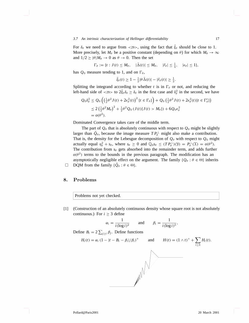
[1] (Construction of an absolutely continuous density whose square root is not absolutelycontinuous.) Fori ≥ 3 define

αi = 1i (log i )2

and βi = 1i (log i )5

,

Define Bi = 2∑

j ≥i βj . Define functions

Hi (t) = αi (1 − |t − Bi − βi |/βi )+ and H(t) = (1 ∧ t)+ +

∑i ≥3

Hi (t).



(i) Show thatBi decreases like(log i )−4.

(ii) Use the fact that∑

i αi < ∞ to prove thatH is absolutely continuous.

(iii) Show thatαi /Bi → 0, then deduce thatH has derivative 1 at 0.

(iv) Show that√

H(Bi −1 − βi ) −√

H(Bi −1) = αi − βi√H(Bi −1 + βi ) + √

H(Bi −1),

which decreases like 1/ i , then deduce thatk+m∑i =k

|√

H(Bi −1 − βi ) −√

H(Bi −1)|

can be made arbitrarily large while keeping∑k+m

i =k |βi | arbitrarily small. Deducethat

√H is not absolutely continuous.

(v) Show, by an appropriate “rounding off of the corners” at each point whereHhas different left and right derivatives followed by some smooth truncation andrescaling, that there exists an absolutely continuous, everywhere differentiableprobability density functionf for which

√f is not absolutely continuous.

[2] Let fθ (x) = 1/2 exp(−|x − θ |), for θ ∈ R (the double-exponential location family ofdensities with respect to Lebesgue measure).

(i) Show that∫ √

fθ (x) fθ+δ(x) dx = (1 + δ/2) exp(−δ/2).

(ii) Deduce that the densityfθ is Hellinger differentiable at everyθ .

(iii) Show thatθ �→ fθ (x) is not differentiable, for each fixedx, at θ = x.

(iv) Prove Hellinger differentiability by a direct Dominated Convergence argument,without the explicit calculation from (i).

(v) Prove Hellinger differentiability by an appeal to Example<24>, without theexplicit calculation from (i).

[3] SupposeF = { fθ : θ ∈ �} is a familiy of densities indexed by a subset�

of Rk. Suppose 0 is an interior point of� and thatF is Hellinger differentiableat θ = 0, with derivative�. Show that�(x) = 0 almost everywhere on{ f0 = 0}.Hint: Approach 0 from each direction inRk. Deduce that bothP0�{ f0 = 0} andP0�

2{ f0 = 0} equal zero.

[4] SupposeF = { ft (x) : t ∈ T} is a family of probability densities with respect toa measureλ, G = {gs(x) : s ∈ S} is a family of probability densities with respectto a measureµ. SupposeF is Hellinger differentiable att = 0 andG is Hellingerdifferentiable ats = 0. Show that the family of densities{ fs(x)gt (y) : (s, t) ∈ S⊗ T}with respect toλ ⊗ µ is Hellinger differentiable at(s, t) = (0, 0). Hint: UseCauchy-Schwarz to bound contributions from most of the cross-product terms in theexpansion of

√ft (x)gs(y).

[5] SupposeF = { fθ : θ ∈ Rk} has Hellinger derivative� at θ0. Show thatF is alsodifferentiable inL1 norm with derivative�1 = 2

√fθ0�, that is, show

λ| fθ − fθ0 − (θ − θ0)′�1| = o(|θ − θ0|) nearθ0


3.8 Problems 19

[6] If F is L1 differentiable andλ f 2/ f0 < ∞ is F also Hellinger differentiable?[Expand.]

[7] Let Pθ be the probability measure defined by the densityfθ (·). A simple applicationof the Cauchy-Schwarz inequality shows that

H(Pθ , Pθ0)2 = (θ − θ0)

′λ(ξ (x)ξ (x)′

)(θ − θ0) + o(|θ − θ0|2).

Provided the matrix� = λ(�(x)�(x)′

)is nonsingular, it then follows that there

exist nonzero constantsC1 andC2 for which

C1|θ − θ0| ≤ H(Pθ , Pθ0) ≤ C2|θ − θ0| nearθ0.

If such a pair of inequalities holds, with fixed strictly positive constantsC1 andC2,throughout some subset of�, then Hellinger distance plays the same role as ordinaryEuclidean distance on that set.

[8] SupposeF = { fθ : θ ∈ �} is a family of probability densities with respect to ameasureλ, with index set� a subset of the real line. As in Theorem<22>, suppose

√fθ+β(x) −

√fθ (x) =

∫ θ+β

θ

�t (x) dt mod[λ], for |β| ≤ δ, a ≤ θ ≤ b,

with supt λ�2t = C < ∞, where [a − δ, b + δ] ⊆ �. Let Q = {qα : −δ < α < δ}

be a family of probability densities with respect to Lebesgue measureµ on [a, b],each bounded by a fixed constantK , and with Hellinger derivativeη at α = 0.Create a new familyP = {pα,β(x, θ) : max(|α|, |β|) < δ} of probability densitiespα,β(x, θ) = qα(θ) fθ+β(x) with respect toλ ⊗ µ.

(i) Show thatP is Hellinger differentiable atα = 0, β = 0 with derivative havingcomponentsη

√fθ and

√f0�θ .

(ii) Try to relax the assumptions onQ.

[9] SupposeP = {Pθ : θ ∈ �}, with 0 ∈ � ⊆ Rk, is a dominated family of probabilitymeasures on a spaceX, having densitiesfθ (x) with respect to a sigma-finitemeasureλ. DefineU as the set of unit vectors

U = {u : there exists a sequence{θi } in � such thatθi /|θi | → u as i → ∞}Write Pθ for the part ofPθ that is absolutely continuous with respect toP0

and P⊥θ = Pθ − Pθ for the part that is singular with respect toP0. Write pθ for the

densitydPθ /d P0.The following are equivalent.

(i) For some vectorξ of functions inL2(λ),√fθ =

√f0 + θ ′ξ + rθ whereλ

(r 2θ

) = o(|θ |2) nearθ = 0,

andu′ξ = 0 a.e. [λ] on { f0 = 0}, for eachu in U.

(ii) For some vector� of functions inL2(P0),√fθ =

√f0 + 2θ ′�

√f0 + Rθ whereλ

(R2

θ

) = o(|θ |2) nearθ = 0,

and P⊥θ X = o(|θ |2).



(iii) For some vector� of functions inL2(P0),√pθ = 1 + 2θ ′� + rθ where P0

(r 2θ

) = o(|θ |2) nearθ = 0,

and P⊥θ X = o(|θ |2).

9. Notes

Incomplete

I borrowed the exposition Section2 from Pollard (1997). The essentialargument is fairly standard, but the interpretation of some of the details is novel.Compare with the treatments of Le Cam (1970, and 1986 Section 17.3), Ibragimov& Has’minskii (1981, page 114), Millar (1983, page 105), Le Cam & Yang (1990,page 101), or Strasser (1985, Chapter 12).

Hajek (1962) used Hellinger differentiability to establish limit behaviour of ranktests for shift families of densities. Most of results in Section6 are adapted from theAppendix to Hajek (1972), which in turn drew on Hájek & Sidak (1967, page 211)and earlier work of Hájek. For a proof of the multivariate version of Theorem<22>

see Bickel et al. (1993, page 13). A reader who is puzzled about all the fuss overnegligible sets, and behaviour at points where the densities vanish, might consultLe Cam (1986, pages 585–590) for a deeper discussion of the subtleties.

The proof of the information inequality (Lemma<13>) is adapted fromIbragimov & Has’minskii (1981, Section 1.7), who apparently gave credit to Blyth& Roberts (1972), but I could find no mention of Hellinger differentiability in thatpaper.

Cite van der Vaart (1988, Appendix A3) and Bickel et al. (1993, page 461) forTheorem<28>. Ibragimov & Has’minskii (1981, page 70) asserted that the resultfollows by “direct calculations”. Indeed my proof uses the same truncation trickas in the proof of Lemma<13>, which is based on the argument of Ibragimov& Has’minskii (1981, page 65). Le Cam & Yang (1988, Section 7) deduced ananalogous result (preservation of DQM under restriction to sub-sigma-fields) byan indirect argument using equivalence of DQM with the existence of a quadraticapproximation to likelihood ratios of product measures (an LAN condition).

References

Bickel, P. J., Klaassen, C. A. J., Ritov, Y. & Wellner, J. A. (1993),Efficient andAdaptive Estimation for Semiparametric Models, Johns Hopkins University Press,Baltimore.

Blyth, C. & Roberts, D. (1972), On inequalities of Cramér-Rao type and admissibilityproofs, in L. Le Cam, J. Neyman & E. L. Scott, eds, ‘Proceedings of the SixthBerkeley Symposium on Mathematical Statistics and Probability’, Vol. I,University of California Press, Berkeley, pp. 17–30.


3.9 Notes 21

Gill, R. & Levit, B. (1995), ‘Applications of the van Trees inequality: a BayesianCramer-Rao bound’,Bernoulli 1, 59–79.

Hajek, J. (1962), ‘Asymptotically most powerful rank-order tests’,Annals ofMathematical Statistics33, 1124–1147.

Hajek, J. (1972), Local asymptotic minimax and admissibility in estimation,inL. Le Cam, J. Neyman & E. L. Scott, eds, ‘Proceedings of the Sixth BerkeleySymposium on Mathematical Statistics and Probability’, Vol. I, University ofCalifornia Press, Berkeley, pp. 175–194.

Hajek, J. &Sidak, Z. (1967),Theory of Rank Tests, Academic Press. Also publishedby Academia, the Publishing House of the Czechoslavak Academy of Sciences,Prague.

Hawkins, T. (1979),Lebesgue’s Theory of Integration: Its Origins and Development,second edn, Chelsea, New York.

Ibragimov, I. A. & Has’minskii, R. Z. (1981),Statistical Estimation: AsymptoticTheory, Springer, New York.

Le Cam, L. (1970), ‘On the assumptions used to prove asymptotic normality ofmaximum likelihood estimators’,Annals of Mathematical Statistics41, 802–828.

Le Cam, L. (1986),Asymptotic Methods in Statistical Decision Theory, Springer-Verlag, New York.

Le Cam, L. & Yang, G. L. (1988), ‘On the preservation of local asymptotic normalityunder information loss’,Annals of Statistics16, 483–520.

Le Cam, L. & Yang, G. L. (1990),Asymptotics in Statistics: Some Basic Concepts,Springer-Verlag.

Le Cam, L. & Yang, G. L. (2000),Asymptotics in Statistics: Some Basic Concepts,2nd edn, Springer-Verlag.

Millar, P. W. (1983), ‘The minimax principle in asymptotic statistical theory’,Springer Lecture Notes in Mathematicspp. 75–265.

Pollard, D. (1997), Another look at differentiability in quadratic mean,in D. Pollard,E. Torgersen & G. L. Yang, eds, ‘A Festschrift for Lucien Le Cam’, Springer-Verlag, New York, pp. 305–314.

Strasser, H. (1985),Mathematical Theory of Statistics: Statistical Experiments andAsymptotic Decision Theory, De Gruyter, Berlin.

van der Vaart, A. (1988),Statistical estimation in large parameter spaces, Center forMathematics and Computer Science. (CWI Tract 44).


Documents

Chapter 3 Hellinger differentiability - Yale Universitypollard/Manuscripts+Notes/Paris2001/Lectures/DQM.pdf · Chapter 3 Hellinger differentiability Modern statistical theory makes