Chapter 3 Implicit Runge-Kutta methods...Chapter 3 Implicit Runge-Kutta methods Although the family of explicit Runga-Kutta methods is quite rich, they may be ine ective for some (particularly

Chapter 3

Implicit Runge-Kuttamethods

Although the family of explicit Runga-Kutta methods is quite rich, they may beineffective for some (particularly hard) problems. Indeed, we will see that no explicitmethod is suitable for so called stiff problems, which frequently arise in practice,in particular from the spatial discretization of time-dependent partial differentialequations. It turns out that implicit methods are much more effective for stiffproblems. However, we will see that the price one has to pay for going implicit isvery high; function evaluations are replaced by the solution of nonlinear systems!

Example 3.1 To solve the IVP

y(t) = 500 y2(1− y), y(0) = 1/100,

we make use of the Matlab function ode23s, which is based on Rosenbrock meth-ods – a variation of implicit Runge-Kutta methods discussed in Section 3.5. Forthis purpose, we need to define the function as well as its derivative (Jacobian) withrespect to y (or an approximation of it):

fun = @(t,y) 500*y^2*(1-y); funjac = @(t,y) 1000*y*(1-y) - 500*y^2;

Additionally to the usual tolerances for the time stepping procedure, the derivativealso needs to be declared in the options:

opt = odeset( ’reltol’, 0.1, ’abstol’, 0.001, ’Jacobian’, funjac );

Finally, the integration is performed on the interval [0, 1]:

[t,x] = ode23s(fun, [0,1], 0.01, opt);

plot(t,x);

From Figure 3.1, it is clear that ode23s requires much less time steps and functionevaluations compared to the explicit Runge-Kutta method in ode23 with the sameoptions. Moreover, ode23s appears to be significantly more accurate than ode23.

27

28 Version March 12, 2015 Chapter 3. Implicit Runge-Kutta methods

0 0.2 0.4 0.6 0.8 10

0.5

1

1.5

t

y

ode23s

0 0.2 0.4 0.6 0.8 10

0.5

1

1.5

t

y

ode23

Figure 3.1. Results of ode23s and ode23 applied to Example 3.1.

3.1 Stability conceptsThe notion of stability is crucial to understand the limitations of explicit methodsfor stiff problems. We consider a linear homogeneous IVP

y(t) = Gy(t), y(t0) = y0, (3.1)

for a d× d matrix G. The IVP (3.1) is called

• asymptotically stable if ‖y(t)‖ → 0 as t→∞ for all initial values y0 ∈ Rd;

• stable if there is a constant C (independent of t and y0) such that ‖y(t)‖ <C‖y0‖ holds for all t ≥ t0 and y0 ∈ Rd;

• unstable, otherwise.

Stability has a number of important consequences. For example if we consider aninhomogeneous problem with undergoing a perturbation of the initial value:

y1(t) = Cy1(t), y1(t0) = y0,

y2(t) = Cy2(t), y2(t0) = y0 +4y0.

then stability implies ‖y1(t) − y2(t)‖ ≤ C‖4y0‖ and asymptotic stability evenimplies that ‖y1(t)− y2(t)‖ → 0. That is, the impact of a perturbation is boundedor vanishes in the long time, respectively.

Let us define the matrix exponential

eB :=∞∑n=0

1

n!Bn, (3.2)

which is absolutely convergent for any B ∈ Cd×d. Then the solution of (3.1) isgiven by

y(t) = eG(t−t0)y0.

3.1. Stability concepts Version March 12, 2015 29

Hence, asymptotic stability is equivalent to ‖eGt‖ → 0 as t → ∞. Stability isequivalent to ‖eGt‖ ≤ C for all t > 0. The following theorem gives a completecharacterization of (asymptotic) stability in terms of the eigenvalues of G. Notethat an eigenvalue λ of G is called semi-simple if its algebraic and geometricmultiplicities are equal or, equivalently, if all blocks in the Jordan canonical formof G associated with λ are 1× 1.

Theorem 3.2 The IVP (3.1) is asymptotically stable if and only if all eigen-values λ of G satisfy Re(λ) < 0.

The IVP (3.1) is stable if and only if all eigenvalues λ of G satisfy Re(λ) ≤ 0and if every eigenvalue λ with Re(λ) = 0 is semi-simple.

Proof. For simplicity, we assume that G is diagonalizable. (The general caserequires to study the Jordan canonical form of A, which is beyond the scope of thislecture.) Then there is an invertible matrix P such that

G = PΛP−1 with Λ =

Öλ1

. . .

λd

è,

where λ1, . . . , λd are the eigenvalues of G. Then

eGt =∞∑n=0

1

n!Gntn =

∞∑n=0

1

n!(PΛP−1)ntn =

∞∑n=0

1

n!PΛnP−1tn

= P eΛtP−1 = P

Öeλ1t

. . .

eλdt

èP−1.

Using that eλt → 0 converges to zero if and only if Re(λ) < 0, it follows that‖eGt‖ → 0 if and only if Re(λ) < 0. This proves the first part.

Moreover, setting C = ‖P−1|2‖P‖2, it follows that

‖eGt‖2 ≤ C‖eΛt‖2 = C · maxλ∈λ1,...,λn

|eλt|,

where the second factor remains bounded (by 1) as t→∞ if and only if Re(λ) ≤ 0.This proves the second part, as the semi-simplicity condition is already containedin the diagonalizability assumption.

To illustrate that the semi-simplicity assumption for critical eigenvalues withRe(λ) = 0 is needed in Theorem 3.2, consider the matrix

G =

Å0 10 0

ã,


which has an eigenvalue 0 that is not semi-simple. Then, by definition (3.2), wehave

eGt =

Å1 t0 1

ã,

which is clearly not bounded as t→∞.We now consider the application of the explicit Euler method with step size h

to (3.1):yi+1 = yi + hGyi = (I + hG)yi. (3.3)

More generally, similar to the proof of Lemma 2.5 it can be shown that the appli-cation of an s-stage explicit Runga-Kutta method applied to (3.1) yields

yi+1 = S(hG)yi (3.4)

for a polynomial S of degree at most s.Both, (3.3) and (3.4) are examples of a linear discrete-time system of the

formyi+1 = Dyi (3.5)

for some matrix D ∈ Rd×d and initial values y0 ∈ Rd. Similar to IVPs, we candefine a notion for the discrete case; (3.5) is called

• asymptotically stable if ‖yk‖ → 0 as k →∞ for all initial values y0 ∈ Rd;

• stable if there is a constant C (independent of t and y0) such that ‖yk‖ <C‖y0‖ holds for all k ≥ 0 and y0 ∈ Rd;

• unstable, otherwise.

Since the solution of (3.5) is clearly yi = Diy0, the stability (3.5) is equivalentlycharacterized by the growth of Di. Analogous to Theorem 3.2, we have the followingeigenvalue characterization.

Theorem 3.3 The linear discrete-time system (3.5) is asymptotically stable ifand only if all eigenvalues λ of D satisfy |λ| < 1.

The linear discrete-time system (3.5) is stable if and only if all eigenvaluesλ of D satisfy |λ| ≤ 1 and if every eigenvalue λ with |λ| = 1 is semi-simple.

3.1.1 Absolute stability

Any one-step method for approximating the solution of an IVP can be seen as adiscrete-time system. The stability of the method is concerned with the followingquestion:

Does the discrete-time system inherit the stability of the IVP?


Re

Im

−3 −2 −1 0 1 2 3−2.5

−2

−1.5

−1

−0.5

0

0.5

1

1.5

2

2.5

Re

Im

−3 −2 −1 0 1 2 3−3

−2

−1

0

1

2

3

Figure 3.2. The green areas denote the stability regions for the forwardEuler method (left plot) and the classical Runga-Kutta method (right plot).

We will study this question for the linear IVP (3.1). In this case, we have alreadyseen that Runge-Kutta methods (and this holds for any linear one-step method)can be written as

yi+1 = S(hG)yi.

for some function S, which is typically a polynomial (in the case of explicit Runge-Kutta methods) or a rational function (in the case of implicit Runge-Kutta methodsdefined below). The question above amounts to investigating whether the eigen-values of S(hG) have absolute magnitude less than 1. Note that the eigenvalues ofS(hG) are given by S(hλ) for every eigenvalue λ of G. Let us therefore define thestability domain as

S := z ∈ C : |S(z)| ≤ 1. (3.6)

Assuming that the IVP is stabble, the method is also stable if

hλ ∈ S

for every eigenvalue λ of G.1

Examples for stability regions are given in Figure 3.2. Note that we have

S(z) = 1 + z +1

2z2 +

1

6z3 +

1

24z4

for the classical Runge-Kutta method (RK4). The best what can happen to ishλ ∈ S no matter how small (or large) h is chosen. Since we are only interested inRe(λ) ≤ 0, this ideal case is guaranteed to happen when C− ⊂ S.

1Since S has to be analytic in a neighborhood of S, an eigenvalue S(hλ) can have modulusone only if hλ ∈ ∂S. The fact that such eigenvalues are semi-simple follows from the fact that amatrix function does not change the block sizes of the Jordan normal form.


Definition 3.4 A method is called A-stable if its stability region S satisfiesC− ⊂ S, where C− denotes the left-half complex plane.

Figure 3.2 clearly shows that neither the explicit Euler nor the classical Runge-Kutta methods are A-stable. More generally, we have the following negative result.

Lemma 3.5 The stability domain S of any explicit Runga-Kutta method is com-pact.

Proof. For an explicit Runga-Kutta method, the function S defining S in (3.6) isa polynomial different of degree at least 1. Since every such polynomial satisfies|S(z)| → ∞ for |z| → ∞, the stability domain must be bounded.

A compact stability domain necessarily imposes a restriction on the step size.The step size for which the ray hλ first leaves S is called critical step size. Undera mild additional assumption2, the critical step size is given by

hc = infh > 0 : hλ 6∈ S. (3.7)

Example 3.6 For the forward Euler method the stability region is a ball of radius1 centered at −1. If G has only real negative eigenvalues, this implies that thecritical step size is given by

hc =2

max|λ| : λ is an eigenvalue of G(3.8)

According to this analysis, the forward Euler method applied to Example 3.1yields the desired asymptotic behavior if |1 − 500h| . 1, that is, h . 1/250. Theobtained approximation for h = 1/100 is displayed in Figure 3.3; it “explodes”after a short time, demonstrating very clearly the risk of choosing h too large. Forh = 1/200, this explosion is avoided, but the correct asymptotic behavior is onlyreflected for h = 1/250 or smaller.

The compactness of the stability region imposes severe restrictions on the stepsize for discretizations of parabolic PDEs. As an illustration, consider the ordinarydifferential equation

·y(t) = Gy(t), with G =1

h2x

à−2 1

1 −2. . .

. . .. . . 1−1 2

í,

2There is the possibility that the ray touches the boundary of the stability domain before, atsome h− < hc. In that case S(h−) has at least one eigenvalue of magnitude 1. If this eigenvalue isnot semi-simple then the critical step size is h−. For simplicity, we do not consider this pathologicalcase.


0 0.2 0.4 0.6 0.8 1−5

0

5

10

15x 10

158

forward Euler, h = 1/100

0 0.2 0.4 0.6 0.8 10

0.5

1

1.5


0 0.2 0.4 0.6 0.8 10

0.5

1

1.5


0 0.2 0.4 0.6 0.8 10

0.5

1

1.5


Figure 3.3. Result of forward Euler applied to Example 3.1 with differentstep sizes h.

which arises from the central finite-difference discretization with mesh width hx ofthe one-dimensional parabolic PDE

∂

∂tu(t, x) =

∂2

∂x2u(t, x), x ∈]0, 1[

u(t, 0) = u(t, 1) = 0.

There are explicit formulas for the eigenvalues of G, which imply that all eigenvaluesare real and negative. Moreover, the smallest eigenvalue satisfies |λ| ∼ h−2

x Hence,according to (3.8), the critical step size of the forward Euler method applied to thisIVP satisfies hc ∼ h2

x. This (highly undesirable) condition is typical when applyingexplicit methods to discretizations of parabolic PDEs.

3.1.2 The implicit Euler method

Since explicit methods always yield polynomial stability function, there is no hopeto obtain an explicit A-stable method. In this section, we will discuss the mostbasic implicit method, the implicit Euler method:

y1 = y0 + hf(t1,y1).


In contrast to explicit methods, we need to solve a system of nonlinear equationsto determine y1! This should be done by the Newton method (or some simplifiedvariant), see Section 3.2.1.

The stability function of the implicit Euler method is given by

S(z) =1

1− z,

and hence the stability region is the complement of a disc in the complex plane, seeFigure 3.4.

3.1.3 Beyond linear ODEs?

Let a general autonomous IVP

y(t) = f(y(t)

), y(t0) = y0, (3.9)

have a stationary point y? and assume that y(t) → y? as t → ∞ for every y0

sufficiently close to y?. Then the linearization around this stationary point takesthe form

y(t) = f ′(u?) · y(t), y(t0) = y0,

where all eigenvalues of the derivative f ′(u?) ∈ Rd×d have negative real part. ARunge-Kutta method with step size h applied to (3.9) converges to y? for sufficientlyclose initial values y0 if λh is in the stability region for every eigenvalue λ of f ′(u?).

A number of crimes are committed when considering the linearization only. Theconcept of B-stability is better suited for nonlinear ODEs; see Chapter IV.12 in[HW].

3.2 General form of implicit Runge-Kutta methodsThe implicit Euler method discussed above belongs to a whole class of implicitRunge-Kutta methods. These are obtained as a generalization of the explicit Runge-Kutta methods, by giving up the requirement that we can compute the stages bymeans of forward substitution.

Definition 3.7 Suppose that k1, . . . ,ks ∈ Rd satisfy the following nonlinearequations:

k1 = f(t0 + c1h,y0 + hs∑`=1

a1`k`)

...

ks = f(t0 + csh,y0 + h

s∑`=1

as`k`

),

3.2. General form of implicit Runge-Kutta methods Version March 12, 2015 35

for given coefficients ai`, ci ∈ R. Then

y1 = y0 + hs∑i=1

biki,

is one step of the s-stage implicit Runge-Kutta method.

Again, the coefficients defining an implicit Runge-Kutta method can be organizedcompactly in a Butcher tableau:

c AbT

:=

c1 a11 · · · · · · a1,s

c2 a21 · · · · · · a2,s

......

...cs as1 · · · · · · ass

b1 · · · · · · bs

Note that in contrast to explicit methods, the matrix A is now a general matrix andnot required to be strictly lower triangular. The three simplest examples of implicitRunge-Kutta methods:

implicit Euler method implicit midpoint rule implicit trapezoidal rule

1 11

1/2 1/21

0 0 01 1/2 1/20 1/2 1/2

The implicit trapezoidal rule has a particularly nice stability region, see Figure 3.4.

For Definition 3.7 to make sense, we need to study the solvability of the systemof nonlinear equations defining the stages. Moreover, some uniqueness propertyof the solutions should be imposed to yield a sensible step. For this purpose, wewill reformulate the system as a system of fixed point equations by introducing thequantities

gi = y0 + hs∑`=1

ai`k`, i = 1, . . . , s.

Then the solutions g1, . . . ,gs of the system of fixed point equations

gi = y0 + hs∑`=1

ai`f(t0 + c`h,g`), i = 1, . . . , s, (3.10)

define the next step as

y1 = y0 + hs∑i=1

bif(t0 + cih,gi), (3.11)


−3 −2 −1 0 1 2 3−3

−2

−1

0

1

2

3

Re

Im

−3 −2 −1 0 1 2 3−3

−2

−1

0

1

2

3

Re

Im

Figure 3.4. Stability regions for the implicit Euler method (left plot) andthe implicit trapezoidal rule (right plot).

This is clearly equivalent to Definition 3.7, as can be seen from the relation

ki = f(t0 + cih,gi), i = 1, . . . , s.

Theorem 3.8 Let f ∈ C(Ω,Rd) be Lipschitz continuous with respect to thestate on the augmented phase space Ω ⊂ R×Rd. Then there exists h∗ > 0 andunique functions gi ∈ C(]− h∗, h∗[,Rd), such that

1. gi(0) = y0 for i = 1, . . . , s;

2. for all 0 ≤ h < h∗, the vectors gi(h) satisfy the equations (3.10).

Proof. We only give a sketch of the proof and refer to Theorem 6.28 in [DB] fordetails. Let us rewrite the system (3.10) as a single equation

g = F (g), with g =

Ög1

...gs

è, F (g) =

Öy0 + h

∑s`=1 a1,`f(t0 + c`h,g`)

...y0 + h

∑s`=1 as`f(t0 + c`h,g`)

è.

(3.12)Then

‖F (g)− F (g)‖∞ ≤ h‖A‖∞ max1≤`≤s

‖f(t0 + c`h, g`)− f(t0 + c`h,g`)‖∞

≤ h‖A‖∞L‖g − g‖∞,

where we used the Lipschitz continuity of f (with Lipschitz constant L). Hence, F


is a contraction provided that

h < h∗ :=1

‖A‖∞L. (3.13)

By the Banach fixed point theorem, this shows the solvability (3.10). To showthe continuous dependence of the solution g on h (and its uniqueness) requires theapplication of a parameter-dependent fixed point theorem, which can be found, e.g.,in [Dieudonne, J. Foundations of Modern Analysis. 1960].

It is interesting to discuss the condition (3.13) on the step size h for a linear ODEy = Gy. Then a suitable Lipschitz constant is given by L = ‖G‖∞. Hence, (3.13)becomes h < 1

‖A‖∞‖G‖∞ , which appears to be a restriction on the step size not better

than the restrictions for explicit methods to be stable! However, this only showsthat fixed point iterations are unsuitable for solving the nonlinear system definingthe stages. For solving the nonlinear system, other methods like the Newton methodshould be used, see also Section 3.2.1.

If we additionally require f ∈ Cp(Ω,Rd) for some p ≥ 1 in Theorem 3.8 thenit can be shown that the vectors gi (and therefore also the step y1) are p timescontinuously differentiable functions in h. This allows to carry over the discussionof Section 2.2.1 on order conditions to implicit Runge-Kutta methods in a nearlyverbatim manner. In particular, an implicit Runge-Kutta method is consistent forall f ∈ C(Ω,Rd) if and only if

bTe = 1.

It is invariant under under autonomization if and only if it is consistent and satisfies

c = Ae.

The order conditions of Theorem 2.12 also apply, only that A(β) is now defined fora general matrix A. Table 2.1 is still valid. The biggest difference is that we nowhave more coefficients available to design the method and potentially achieve higherorder. In fact, the order can be larger than s (but not larger than 2s). For example,the implicit midpoint rule has order 2.

Finally, we give a compact formula for the stability function of an implicit Runge-Kutta method.

Lemma 3.9 The stability function of an s-stage implicit Runge-Kutta method isgiven by

S(z) = 1 + zbT(I − zA)−1e,

which is a rational function.

Proof. When applying the implicit Runge-Kutta method to the linear IVP y(t) =λy(t) we obtain from (3.12) the linear system

g = y0e + hλAg

and hence g = y0(I − hλA)−1e. According to (3.11) the next step is given by

y1 = y0 + y0hλbT(I − hλA)−1e = (1 + hλbT(I − hλA)−1e)︸︷︷︸

=S(hλ)

y0.


This shows the first statement. The second statement follows from the fact thatthe entries of (I − zA)−1 are rational functions in z, which is a consequence of(I − zA)−1 = adj(I − zA)/det(I − zA).

3.2.1 Solution of the nonlinear system defining the stages

The implementation of an implicit Runge-Kutta method requires the solution ofthe nonlinear equations (3.10). Since gi − y0 = O(h) there is the risk of numericalcancellation for small step sizes h. It is therefore preferable to work with the smallerquantities

zi := gi − y0.

Then (3.10) becomes

zi = hs∑`=1

ai`f(t0 + c`h,y0 + z`), i = 1, . . . , s,

which can be written as

z :=

Öz1

...zs

è= (A⊗ I)

Öhf(t0 + c1h,y0 + z1)

...hf(t0 + csh,y0 + zs)

è=: (A⊗ I)F (z), (3.14)

where ⊗ denotes the Kronecker product between two matrices. Once z1, . . . , zs aredetermined, we could then determine the next step by

y1 = y0 + hs∑i=1

bif(t0 + cih,y0 + zi),

This seems to suggest that s additional function evaluations are needed. In factthis can be avoided with a small trick. Assuming that A is invertible, it followsfrom (3.14) that we can write

y1 = y0 +s∑i=1

dizi,

where (d1, . . . , ds

):= bTA−1.

The kth step of the Newton method applied to the nonlinear system (3.14)takes the following form:

Solve linear system(I − (A⊗ I)F ′(zk)

)4zk = −zk + h(A⊗ I)F (zk),

Update zk+1 = zk +4zk.(3.15)


Note that each step of (3.15) requires to solve a linear system. In practice, thisis usually done via computing a (sparse) LU factorization of the matrix

I − (A⊗ I)F ′(zk)

=I − h

Üa11

∂f∂y (t0 + c1h,y0 + zk1) · · · a1s

∂f∂y (t0 + c1h,y0 + zks)

......

as1∂f∂y (t0 + csh,y0 + zk1) · · · ass

∂f∂y (t0 + csh,y0 + zks)

ê.

The factorization of this sd × sd matrix is often the (by far) most expensive partand needs to be performed in every step of the Newton method (3.15).

We can reduce the cost significantly by, replacing all Jacobians ∂f∂y (t0 + c1h,y0 +

zks) with an approximation

J ≈ ∂f

∂y(t0,y0).

The resulting simplified Newton method takes the form:

Solve linear system(I − (A⊗ I)J

)4zk = −zk + h(A⊗ I)F (zk),

Update zk+1 = zk +4zk.(3.16)

Now, the LU factorization of I − (A⊗ I)J needs to be computed only once and canthen be reused. Hence, we only need to perform 1 LU factorization in each step ofthe implicit Runge-Kutta method.

The choice

z0 = 0

usually represents a very good starting value, since the exact solution is known tosatisfy ‖z‖ = O(h). Suggestions for better starting values can be found in SectionIV.8 of [HW], which also discusses a suitable stopping criterion for (3.16).

3.2.2 Examples of implicit Runge-Kutta methods

As described in [DB] and [HW], collocation combined with numerical quadratureprovides a way to construct high-order implicit Runge-Kutta methods.

Gauss methods. Gauss quadrature yields s-stage implicit Runge-Kutta methodsthat are A-stable and have order 2s (which is optimal). For s = 1, the Gaussmethod coincides with the implicit midpoint rule. For s = 2, the Gauss method hasthe following Butcher tableau:

12 −

√3

614

14 −

√3

6

12 +

√3

614 +

√3

614

12

12


−15 −10 −5 0 5 10 15−15

−10

−5

0

5

10

−1 −0.5 0 0.5 1−1

−0.5

0

0.5

Figure 3.5. Forward Euler (left plot) and implicit Euler (right plot) appliedto (3.17).

Radau methods. Radau quadrature yields s-stage implicit Runge-Kutta methodsthat are A-stable and have order 2s−1. Moreover, Radau methods have a propertycalled L-stability, see Section 3.4 below. For s = 1, the Radau method is our goodold friend – the implicit Euler method. For s = 2 and s = 3, the Radau methodshave the following Butcher tableaus:

13

512 − 1

12

1 34

14

34

14

0 19

−1−√

618

−1+√

618

6−√

610

19

88+7√

6360

88−43√

6360

6+√

610

19

88+43√

6360

88−7√

6360

19

16+√

636

16−√

636

RADAU5, one of the most popular codes for solving DAEs, is based on the 3-stageRadau method.

3.3 The danger of being too stableDespite all the praise for A-stable methods, they actually bear the danger of turn-ing an unstable or a non-asymptotically stable IVP into an asymptotically stablediscrete-time system. This point is nicely illustrated with

y(t) =

Å0 1−1 0

ãy(t), y(0) =

Å10

ã=: y0, (3.17)

which arises, e.g., from the model of a spring pendulum. The solution stays onthe unit circle and does not converge to a stationary point. Figure 3.5 displaysthe approximations on the interval [0, 10] obtained from the forward/implicit Eulermethods with step size h = 1/10. It can be seen that the forward Euler methoddoes not stay on the unit circle and the solution drifts away as t increases. This

is not unexpected: The eigenvalues of the matrix A =

Å0 1−ω2 0

ãare λ = ±ωi.

3.4. L-stability Version March 12, 2015 41

−1 −0.5 0 0.5 1−1

−0.5

0

0.5

1

−1 −0.5 0 0.5 1−1

−0.5

0

0.5

1

Figure 3.6. Implicit trapezoidal method with h = 1 (left plot) and h = 0.1(right plot) applied to (3.17).

Hence, no matter how small h is, hλ is not in the stability region of the forwardEuler method. Unfortunately, the behavior of the implicit Euler method is notmuch better. The solution does also not stay on the unit circle and approacheszero for long times. Ironically, the problem is now that hλ is in the interior ofthe stability region of the implicit Euler method. Thus, the approximate solutionalways converges to zero, no matter how small h is.

To avoid the phenomena described above, we need a method for which hλ ison the boundary of the stability region. Such a method is given by the trape-zoidal method, see Figure 3.4. Indeed, this method produces the exact asymptoticbehavior even for relatively large h, see Figure 3.6.

3.4 L-stabilitySection 3.3 may misleadingly indicate that it is always desirable to have the stabilityregion coincide with the left half-plane. In fact, for very stiff problems this is notdesirable at all. For a rational stability function S, we have

limx→−∞

S(x) = limx→∞

S(x) = limy→∞

S(iy).

If the stability region coincide with the left half-plane, then |S(iy)| = 1 for all y ∈ R.In turn, |S(z)| is close to 1 whenever z is close to the real axis and has large negativereal part. In practice, this means that such a method damps errors only very slowlyfor stiff problems. To see this, let us consider the IVP

y(t) = −2000(y(t)− cos t), y(0) = 0. (3.18)

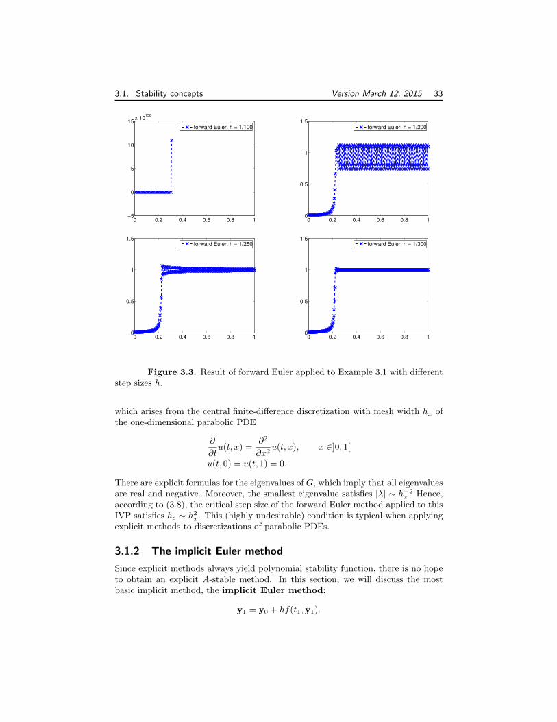
As can be seen from Figure 3.7, the initial numerical oscillation is damped muchmore quickly for the implicit Euler method compared to the trapezoidal method.This is due to the following property.

Definition 3.10 A method is called L-stable if it is A-stable and if, additionally,

limx→∞

R(x) = 0.


0 0.5 1 1.5−0.5

0

0.5

1

1.5

2

imp. Eulerimp. trapezoidal

Figure 3.7. Implicit Euler and implicit trapezoidal method with h = 1.5/40applied to (3.18).

For an implicit Runge-Kutta method defined by b, c, A with nonsingular A, we have

S(∞) = 1− bTA−1e,

where e is the vector of all ones. Hence, the method is L-stable if and only ifbTA−1e = 1. Examples of L-stable methods include the implicit Euler method andthe Radau methods mentioned above.

Apart from stiff ODEs, L-stability also plays an important role when solvingdifferential-algebraic equations (DAEs), that is, ODEs with additional algebraicside constraints.

3.5 Rosenbrock methods?

When using the simplified Newton method (3.16), one has to strike a balance be-tween the stopping criterion the inner iterations and h. It would be much simplerif we could just use one iteration and let the accuracy be handled solely by the stepsize control for the Runge-Kutta method. Rosenbrock methods (also called lin-early implicit Runge-Kutta methods) rationalize this idea. They can be motivatedby considering an implicit Runge-Kutta method with a lower triangular matrix Aapplied to an autonomous ODE:

ki = f(y0 + h

i−1∑`=1

ai`k` + aiiki

), i = 1, . . . , s,

y1 = y0 + hs∑i=1

biki.

3.5. Rosenbrock methods? Version March 12, 2015 43

Such a method is also called DIRK (diagonally implicit Runge-Kutta method).Linearizing this formula in order to get rid off the implicit part yields

ki = f(gi) + hf ′(gi)aiiki,

where

gi = y0 + hi−1∑`=1

ai`k`

for i = 1, . . . , s. This is one step of the Newton method. Now we replace f ′(gi) byJ = f ′(y0) and obtain one step of the simplified Newton method. Some additionalfreedom is gained by allowing for linear combinations of Jk`.

Definition 3.11 An s-stage Rosenbrock method is defined by

ki = f(y0 + h

i−1∑`=1

ai`k`

)+ hJ

i∑`=1

γi`k`, i = 1, . . . , s,

y1 = y0 + hs∑i=1

biki,

with coefficients αi`, γi`, bi and J = f ′(y0).

Note that each stage of the Rosenbrock method requires to solve a linear systemwith the matrix I − hγiiJ . Naturally, methods with γ11 = · · · = γss ≡ γ are ofparticular interest, because they allow to reuse the LU factorization of I − hγJwhen having to solve the linear system for each stage. We refer to Section IV.7 in[HW] for the construction of specific Rosenbrock methods.

A particularly simple example of a Rosenbrock method is given by:

(I − hγJ)k1 = f(y0), γ =1

2 +√

2,

(I − hγJ)k2 = f(y0 +

1

2hk1

)− hγJk1

y1 = y1 + hk2.

A modified variant of this second-order method is behind Matlab’s ode23s; see[L. F. Shampine and M. W. Reichelt: The Matlab ODE suite] for more details.

Documents

Chapter 3 Implicit Runge-Kutta methods...Chapter 3 Implicit Runge-Kutta methods Although the family of explicit Runga-Kutta methods is quite rich, they may be ine ective for some (particularly