Chapter 3 - Interest and Equivalence Click here for Streaming Audio To Accompany Presentation (optional) Click here for Streaming Audio To Accompany Presentation

Chapter 3 - Interest and Equivalence

Click here for Streaming Audio To Accompany Presentation (optional)

EGR 403 Capital Allocation Theory

Dr. Phillip R. RosenkrantzIndustrial & Manufacturing Engineering Department

Cal Poly Pomona

http://video.csupomona.edu/PRRosenkrant/EGR403Lecture-05.asx



EGR 403 - Cal Poly Pomona - SA5 2

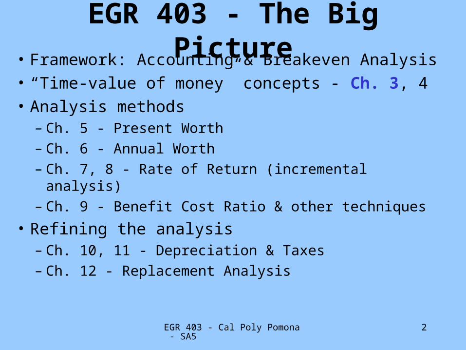
EGR 403 - The Big Picture• Framework: Accounting & Breakeven Analysis

• “Time-value of money” concepts - Ch. 3, 4

• Analysis methods– Ch. 5 - Present Worth– Ch. 6 - Annual Worth– Ch. 7, 8 - Rate of Return (incremental analysis)– Ch. 9 - Benefit Cost Ratio & other techniques

• Refining the analysis– Ch. 10, 11 - Depreciation & Taxes– Ch. 12 - Replacement Analysis


Economic Decision Components

• Where economic decisions are immediate we need to consider:– amount of expenditure– taxes

• Where economic decisions occur over a considerable period of time we need to also consider the consequences of:– interest– inflation


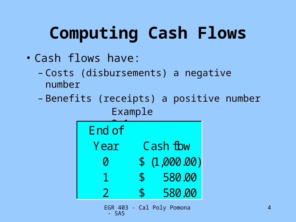
Computing Cash Flows

• Cash flows have:– Costs (disbursements) a negative number– Benefits (receipts) a positive number

Example 3-1

End of Year Cash flow

0 (1,000.00)$ 1 580.00$ 2 580.00$


Time Value of Money

• Money has value– Money can be leased or rented

– The payment is called interest

– If you put $100 in a bank at 9% interest for one time period you will receive back your original $100 plus $9

Original amount to be returned = $100Interest to be returned = $100 x .09 = $9


Simple Interest

• Interest that is computed only on the original sum or principal

• Total interest earned = I = P i n , where:– P = present sum of money, or “principal” (example:

$1000)– i = interest rate (10% interest is a .10 interest rate)– n = number of periods (years) (example: n = 2 years)

I = $1000 x .10/period x 2 periods = $200


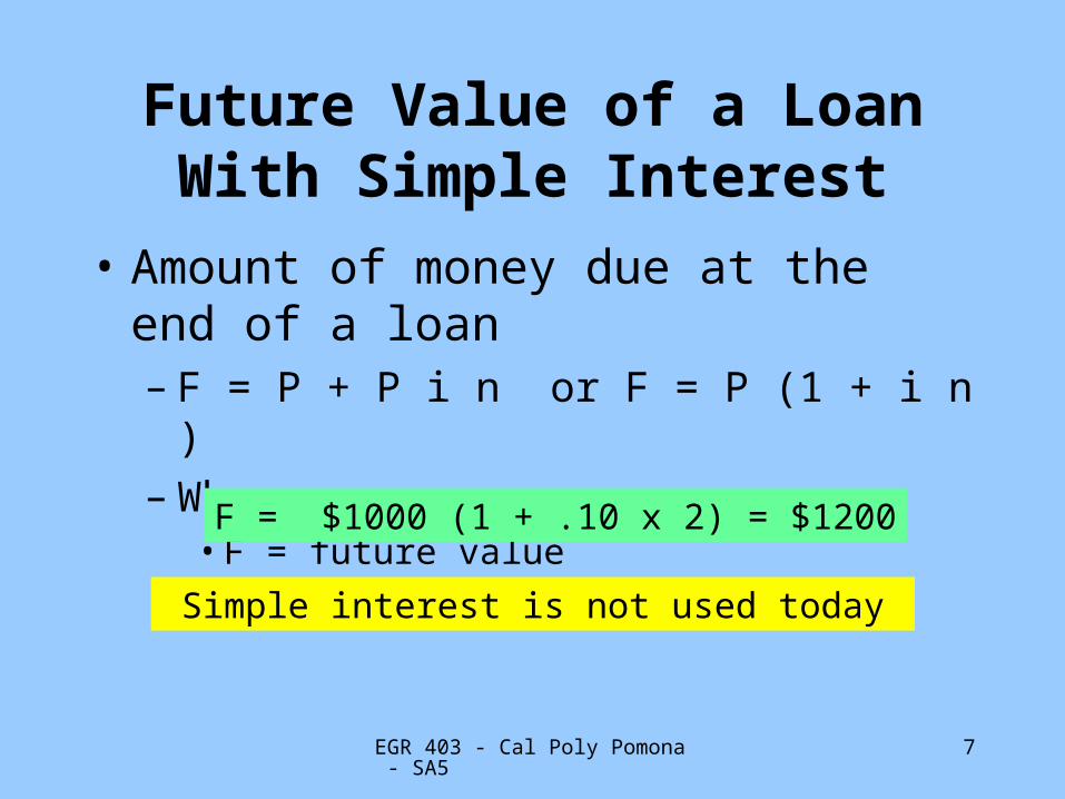
Future Value of a Loan With Simple Interest

• Amount of money due at the end of a loan– F = P + P i n or F = P (1 + i n )– Where,

• F = future value

F = $1000 (1 + .10 x 2) = $1200

Simple interest is not used today


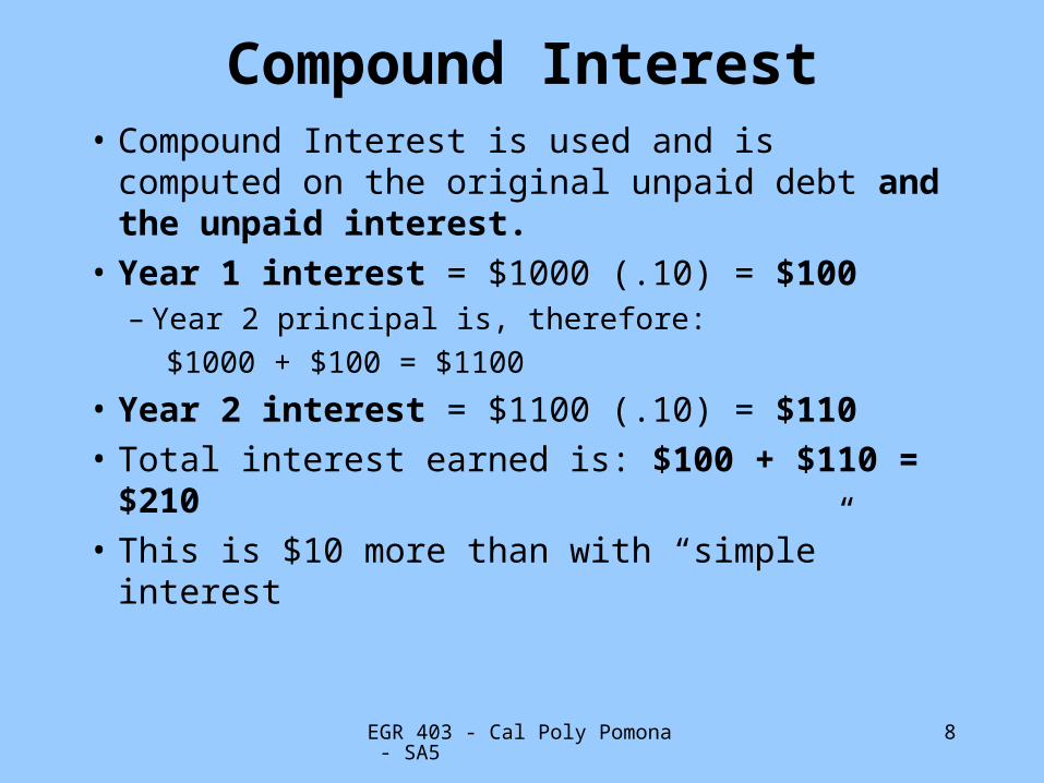
Compound Interest• Compound Interest is used and is computed on

the original unpaid debt and the unpaid interest.

• Year 1 interest = $1000 (.10) = $100– Year 2 principal is, therefore:

$1000 + $100 = $1100

• Year 2 interest = $1100 (.10) = $110

• Total interest earned is: $100 + $110 = $210

• This is $10 more than with “simple” interest


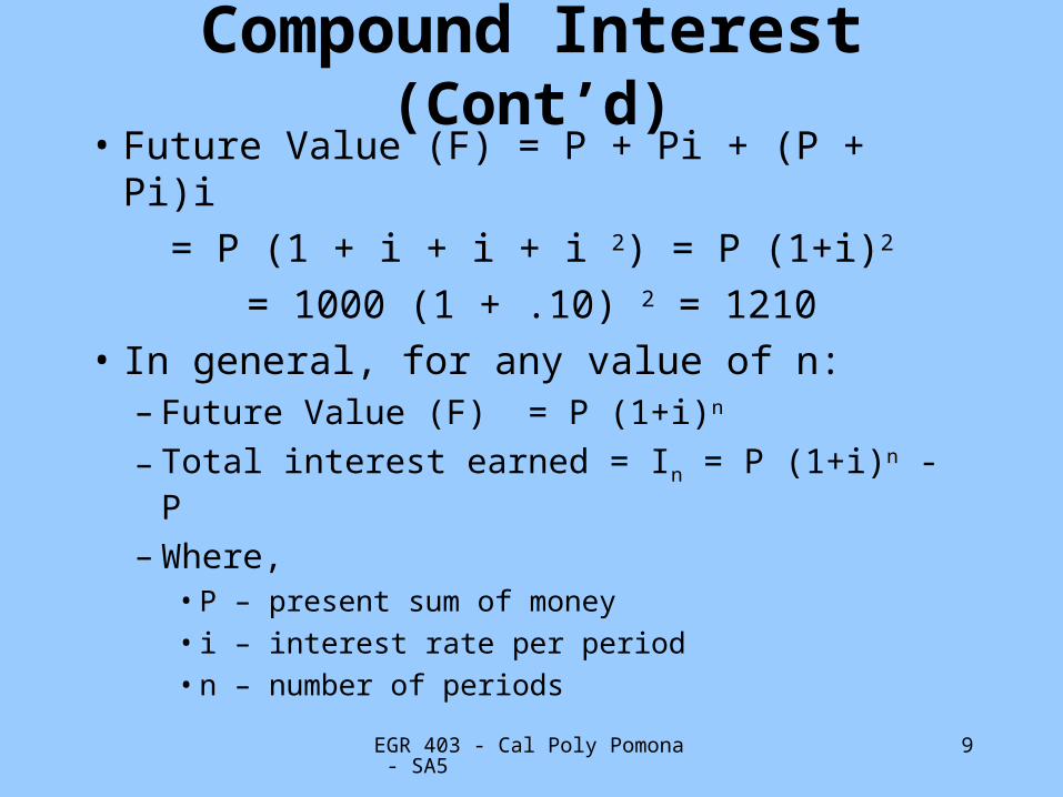
Compound Interest (Cont’d)• Future Value (F) = P + Pi + (P + Pi)i

= P (1 + i + i + i 2) = P (1+i)2

= 1000 (1 + .10) 2 = 1210

• In general, for any value of n:– Future Value (F) = P (1+i)n

– Total interest earned = In = P (1+i)n - P

– Where, • P – present sum of money

• i – interest rate per period

• n – number of periods


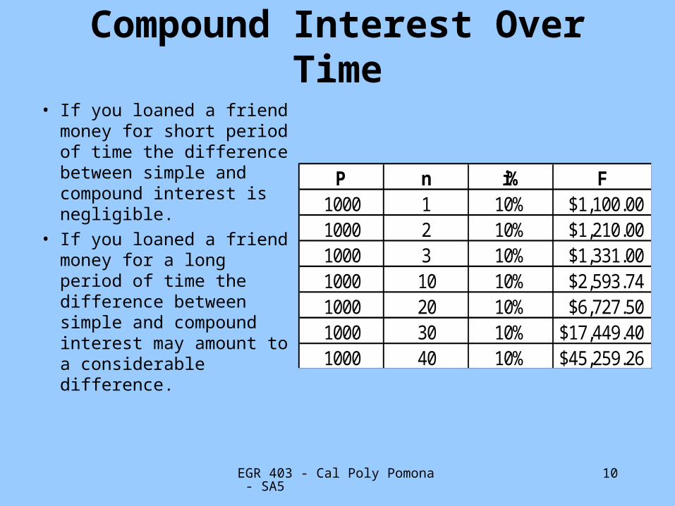
Compound Interest Over Time

• If you loaned a friend money for short period of time the difference between simple and compound interest is negligible.

• If you loaned a friend money for a long period of time the difference between simple and compound interest may amount to a considerable difference.

P n i% F1000 1 10% $1,100.001000 2 10% $1,210.001000 3 10% $1,331.001000 10 10% $2,593.741000 20 10% $6,727.501000 30 10% $17,449.401000 40 10% $45,259.26


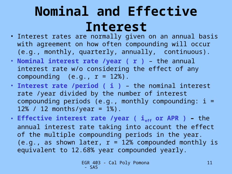
Nominal and Effective Interest• Interest rates are normally given on an annual basis with

agreement on how often compounding will occur (e.g., monthly, quarterly, annually, continuous).

• Nominal interest rate /year ( r ) – the annual interest rate w/o considering the effect of any compounding (e.g., r = 12%).

• Interest rate /period ( i ) – the nominal interest rate /year divided by the number of interest compounding periods (e.g., monthly compounding: i = 12% / 12 months/year = 1%).

• Effective interest rate /year ( ieff or APR ) – the annual interest rate taking into account the effect of the multiple compounding periods in the year. (e.g., as shown later, r = 12% compounded monthly is equivalent to 12.68% year compounded yearly.


Interest Rates (cont’d)

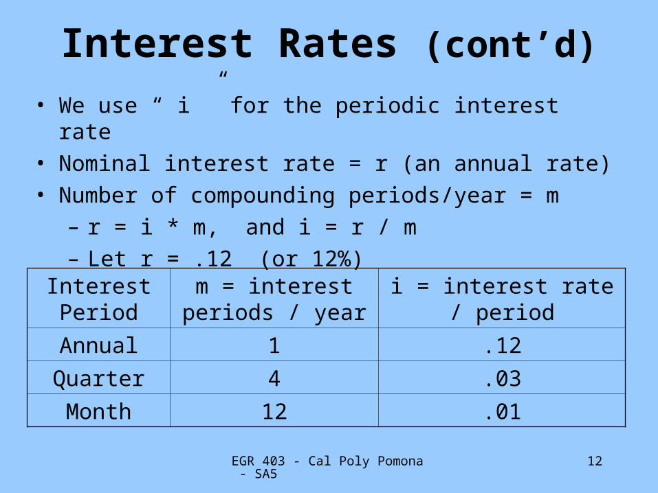
• We use “ i ” for the periodic interest rate

• Nominal interest rate = r (an annual rate)

• Number of compounding periods/year = m

– r = i * m, and i = r / m

– Let r = .12 (or 12%)

Interest Period m = interest periods / year

i = interest rate / period

Annual 1 .12

Quarter 4 .03

Month 12 .01


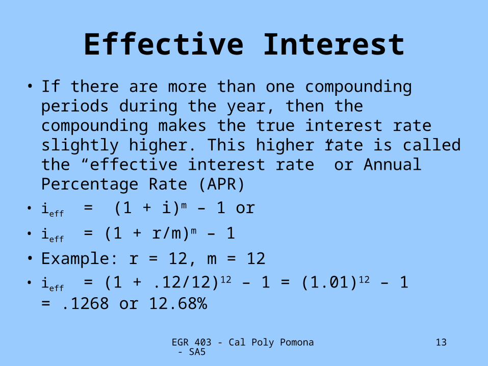
Effective Interest• If there are more than one compounding periods during

the year, then the compounding makes the true interest rate slightly higher. This higher rate is called the “effective interest rate” or Annual Percentage Rate (APR)

• ieff = (1 + i)m – 1 or

• ieff = (1 + r/m)m – 1

• Example: r = 12, m = 12

• ieff = (1 + .12/12)12 – 1 = (1.01)12 – 1 = .1268 or 12.68%


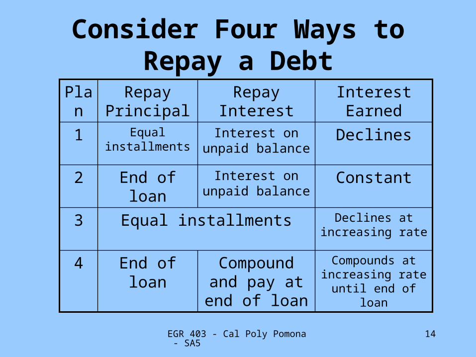
Consider Four Ways to Repay a Debt

Compound and pay at end of

loan

Interest on unpaid balance

Interest on unpaid balance

Repay Interest

Declines at increasing rate

Equal installments3

Compounds at increasing rate

until end of loan

End of loan4

ConstantEnd of loan2

DeclinesEqual installments

1

Interest EarnedRepayPrincipal

Plan


Plan 1 – Equal annual principal payments

Year Balance P i Payment

1 5000 1000 500 1500

2 4000 1000 400 1400

3 3000 1000 300 1300

4 2000 1000 200 1200

5 1000 1000 100 1100

6500


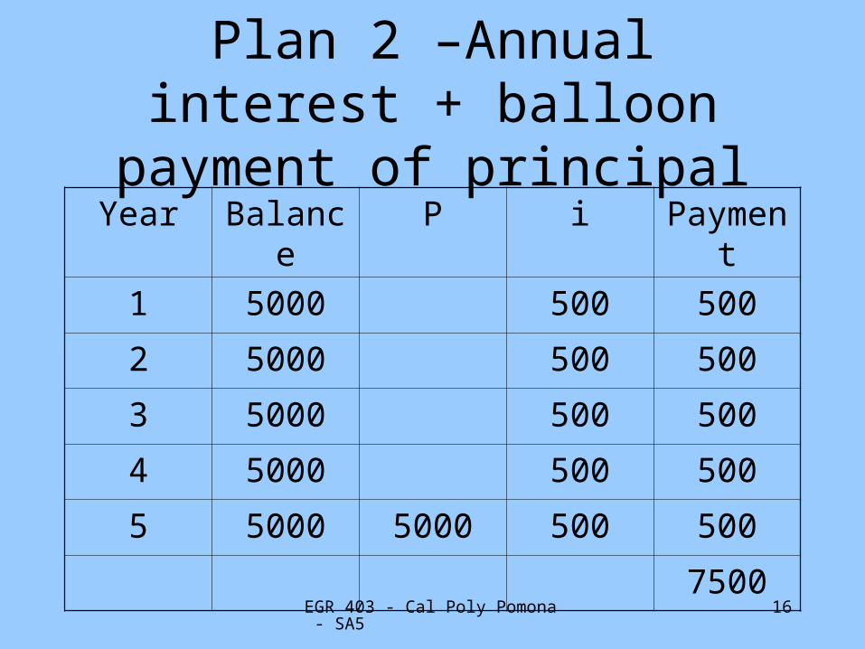
Plan 2 –Annual interest + balloon payment of principal


1 5000 500 500

2 5000 500 500

3 5000 500 500

4 5000 500 500

5 5000 5000 500 500

7500


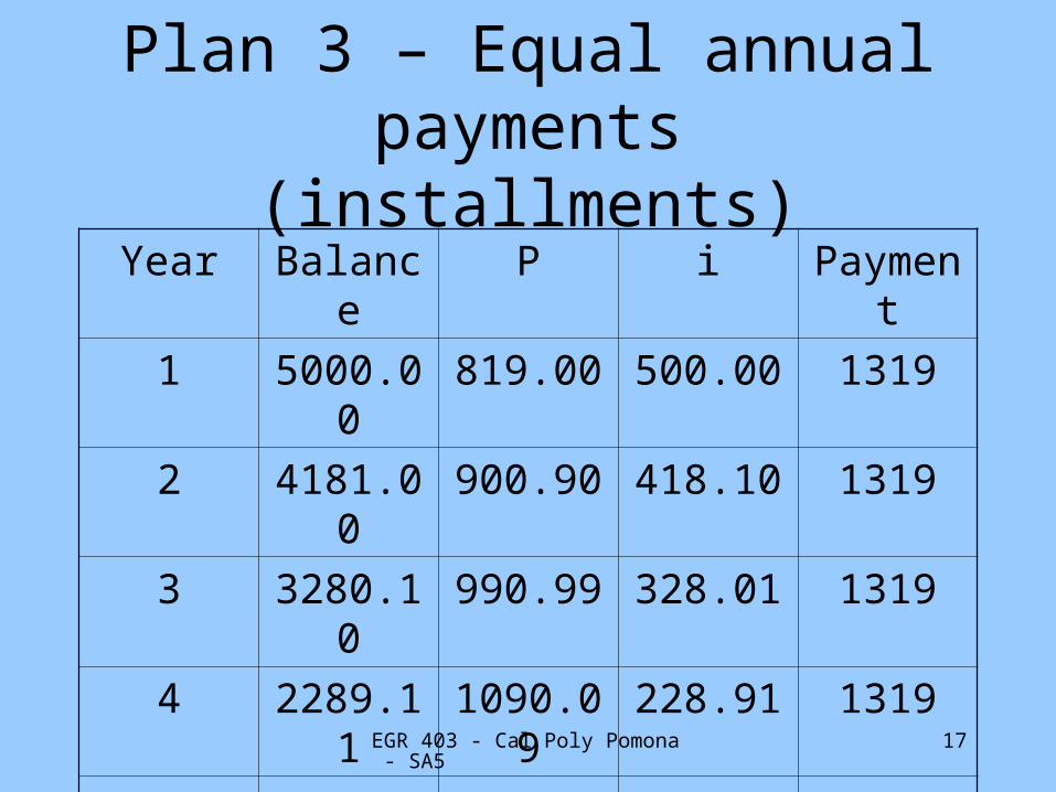
Plan 3 – Equal annual payments (installments)


1 5000.00 819.00 500.00 1319

2 4181.00 900.90 418.10 1319

3 3280.10 990.99 328.01 1319

4 2289.11 1090.09 228.91 1319

5 1199.02 1199.10 119.90 1319

6595


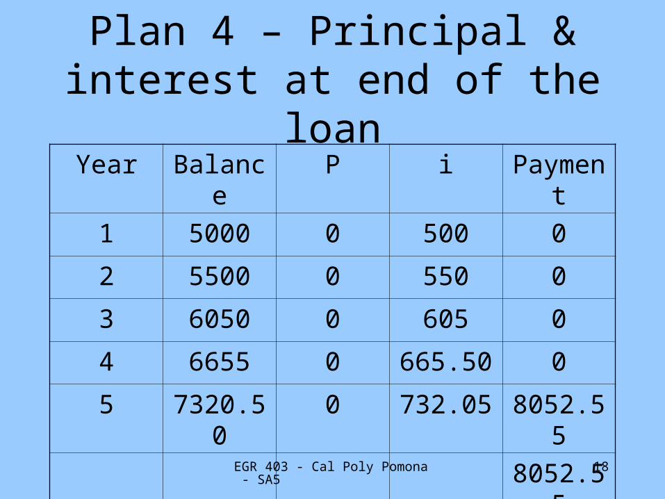
Plan 4 – Principal & interest at end of the loan


1 5000 0 500 0

2 5500 0 550 0

3 6050 0 605 0

4 6655 0 665.50 0

5 7320.50 0 732.05 8052.55

8052.55


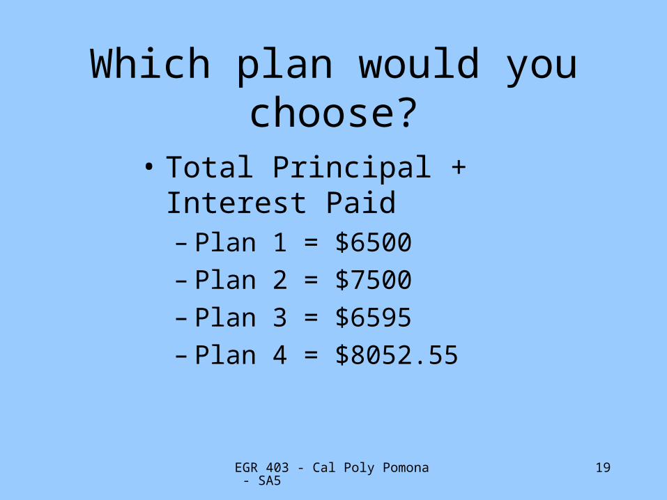
Which plan would you choose?

• Total Principal + Interest Paid– Plan 1 = $6500– Plan 2 = $7500– Plan 3 = $6595– Plan 4 = $8052.55


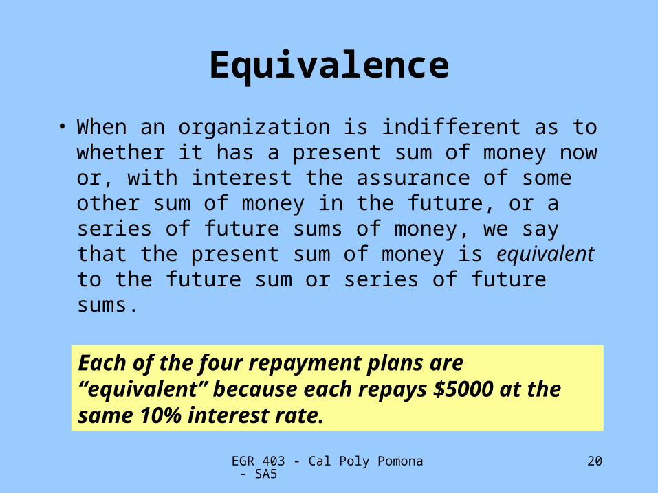
Equivalence

• When an organization is indifferent as to whether it has a present sum of money now or, with interest the assurance of some other sum of money in the future, or a series of future sums of money, we say that the present sum of money is equivalent to the future sum or series of future sums.

Each of the four repayment plans are “equivalent” because each repays $5000 at the same 10% interest rate.


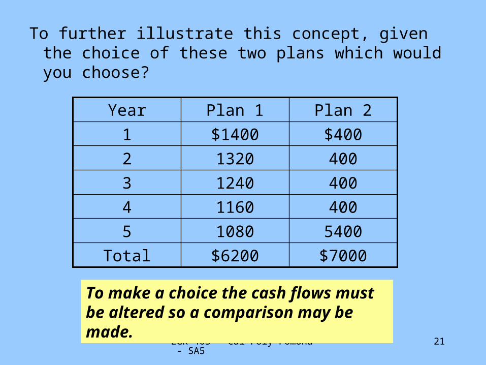
To further illustrate this concept, given the choice of these two plans which would you choose?

$7000$6200Total

540010805

40011604

40012403

40013202

$400$14001

Plan 2Plan 1Year

To make a choice the cash flows must be altered so a comparison may be made.


Technique of Equivalence• Determine a single equivalent value at a

point in time for plan 1.• Determine a single equivalent value at a

point in time for plan 2.

Both at the same interest rate

Judge the relative attractiveness of the two alternatives from the comparable equivalent values. You will learn a number of methods for finding comparable equivalent values.


Analysis Methods that Compare Equivalent Values

• Present Worth Analysis (Ch. 5) - Find the equivalent value of cash flows at time 0.

• Annual Worth Analysis (Ch. 6) - Find the equivalent annual worth of all cash flows.

• Rate of Return Analysis (Ch. 7, 8) - Compare the interest rate (ROR) of each alternative’s cash flows to a minimum value you will accept.

• Future Worth Analysis (Ch. 9) - Find the equivalent value of cash flows at time in the future.

• Benefit/Cost Ratio (Ch. 9) - Use equivalent values of cash flows to form ratios that can be easily analyzed.


Interest Formulas• To understand equivalence the underlying

interest formulas must be analyzed. We will start with “Single Payment” interest formulas.

• Notation:i = Interest rate per interest period.

n = Number of interest periods.

P = Present sum of money (Present worth, PV).

F = Future sum of money (Future worth, FV).

• If you know any three of the above variables you can find the fourth one.


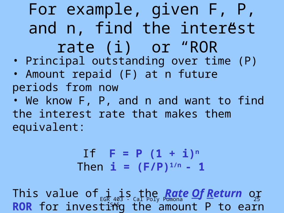
For example, given F, P, and n, find the interest rate (i) or “ROR”

• Principal outstanding over time (P)• Amount repaid (F) at n future periods from now• We know F, P, and n and want to find the interest rate that makes them equivalent:

If F = P (1 + i)n

Then i = (F/P)1/n - 1

This value of i is the Rate Of Return or ROR for investing the amount P to earn the future sum F


Functional Notation• Give P, n, and i, we can solve for F several ways:

– Use the formula and a calculator– Use the factors and functional notation in the tables

in the back of the text

– Use the financial functions (fx) in EXCEL

– Use the financial functions available in many calculators

• In this course we will use the factors or EXCEL spreadsheet functions unless otherwise instructed


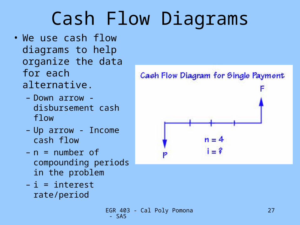
Cash Flow Diagrams• We use cash flow

diagrams to help organize the data for each alternative. – Down arrow -

disbursement cash flow

– Up arrow - Income cash flow

– n = number of compounding periods in the problem

– i = interest rate/period


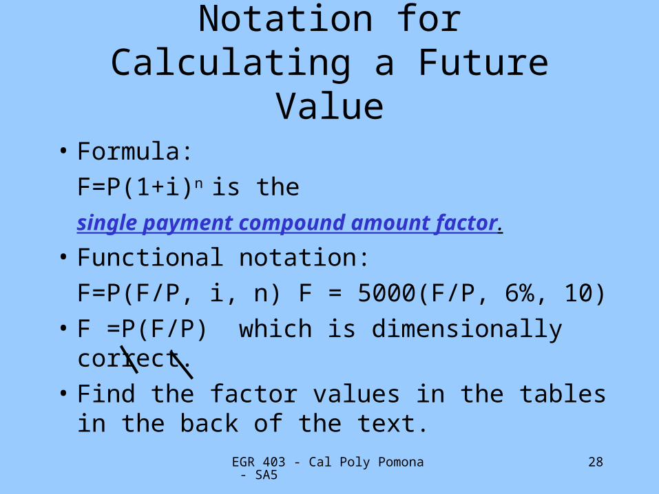
Notation forCalculating a Future Value

• Formula:

F=P(1+i)n is the

single payment compound amount factor.

• Functional notation:

F=P(F/P, i, n) F = 5000(F/P, 6%, 10)• F =P(F/P) which is dimensionally correct.• Find the factor values in the tables in the back

of the text.


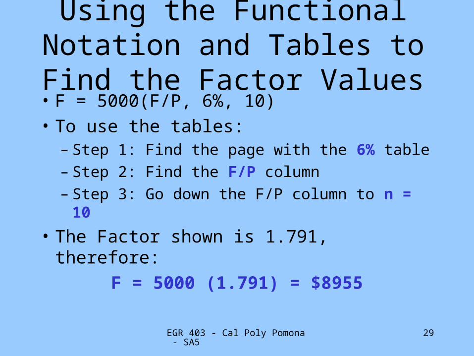
Using the Functional Notation and Tables to Find the Factor Values• F = 5000(F/P, 6%, 10)

• To use the tables:– Step 1: Find the page with the 6% table– Step 2: Find the F/P column– Step 3: Go down the F/P column to n = 10

• The Factor shown is 1.791, therefore:

F = 5000 (1.791) = $8955


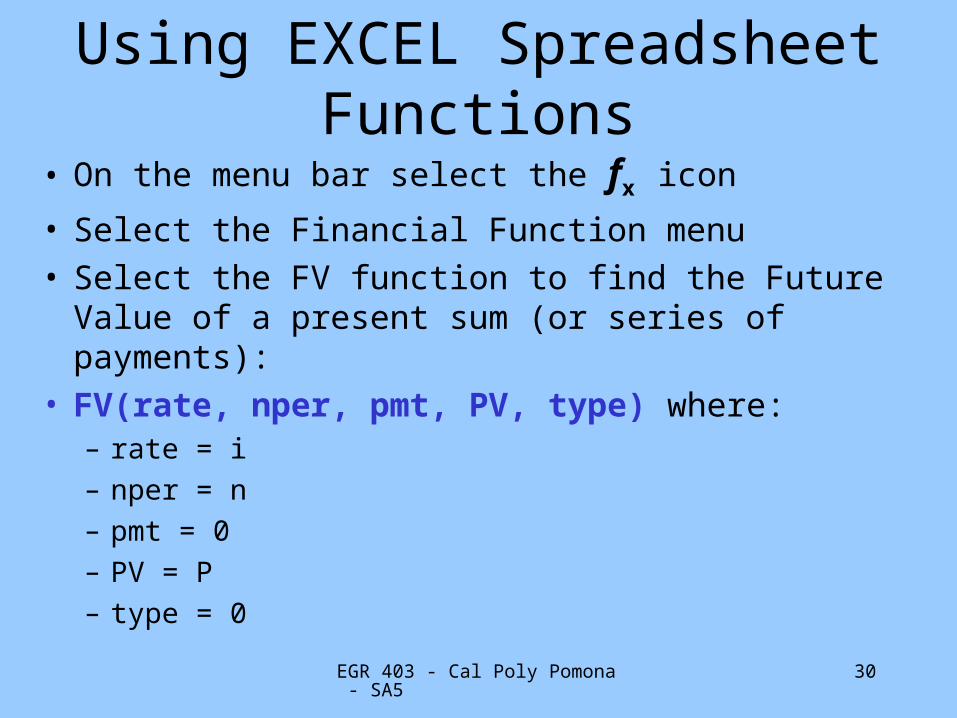
Using EXCEL Spreadsheet Functions

• On the menu bar select the fx icon

• Select the Financial Function menu• Select the FV function to find the Future Value of a

present sum (or series of payments): • FV(rate, nper, pmt, PV, type) where:

– rate = i

– nper = n

– pmt = 0

– PV = P

– type = 0


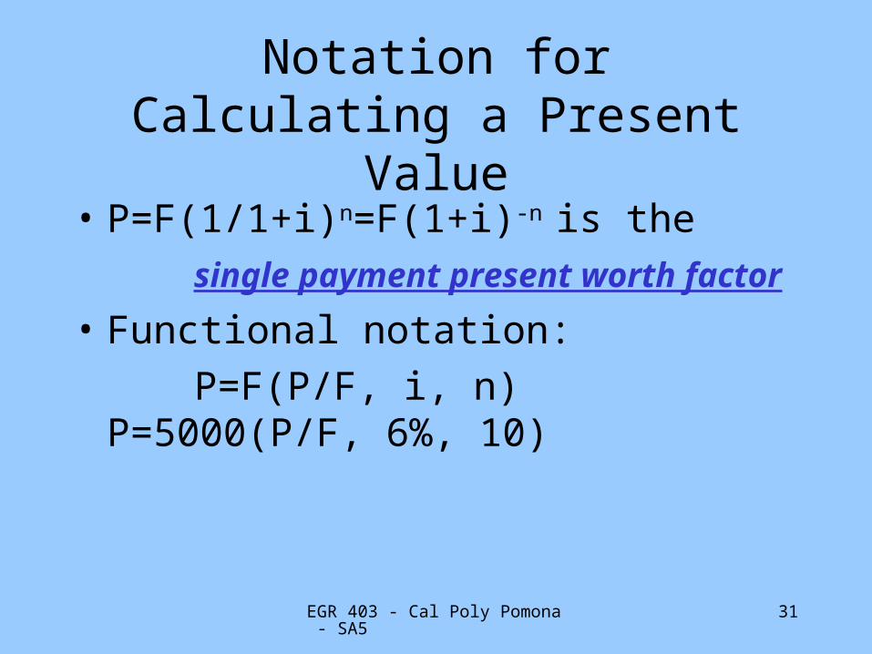
Notation forCalculating a Present Value

• P=F(1/1+i)n=F(1+i)-n is the

single payment present worth factor

• Functional notation:

P=F(P/F, i, n) P=5000(P/F, 6%, 10)


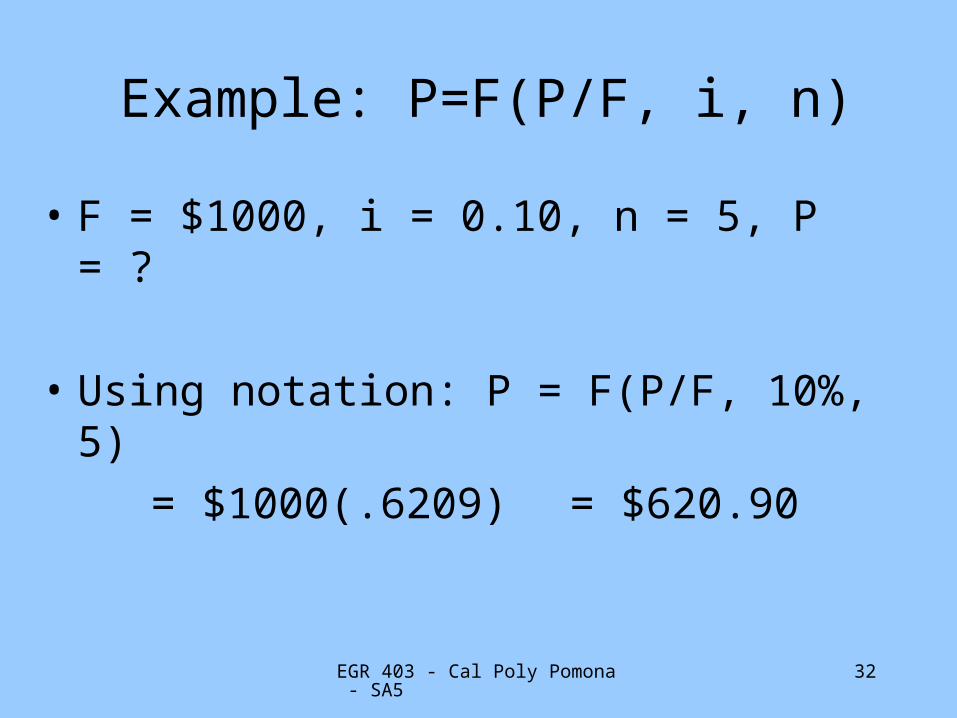
Example: P=F(P/F, i, n)

• F = $1000, i = 0.10, n = 5, P = ?

• Using notation: P = F(P/F, 10%, 5)

= $1000(.6209) = $620.90

Documents

Chapter 3 - Interest and Equivalence Click here for Streaming Audio To Accompany Presentation (optional) Click here for Streaming Audio To Accompany Presentation