CHAPTER 3 LABORATORY TESTING PROGRAM 3.1 Description of

32

CHAPTER 3

LABORATORY TESTING PROGRAM

3.1 Description of Laboratory Testing Program

Review of the literature indicates that there is very little published information on stress-

strain properties of soil-bentonite mixtures. Consequently, a laboratory testing program

with the following objectives was completed: 1) to add to the body of knowledge on

stress-strain properties of soil-bentonite mixtures and 2) to provide information useful for

choosing an appropriate constitutive model for soil-bentonite. The test procedures and

results are presented in this chapter. Interpretation of the tests to evaluate constitutive

models is presented in Chapter 4.

Three soil-bentonite mixtures were fabricated for the laboratory testing program. They

are referred to as SB1, SB2, and SB3. SB1 and SB2 are identical except that SB1 was

made with distilled water and SB2 was made with tap water. SB2 was created for hy-

draulic conductivity tests since tap water is recommended over distilled water for hydrau-

lic conductivity testing (Daniel 1994). SB3 was also made with tap water. An extensive

lab testing program was performed on SB1 to fully characterize its material properties.

The following tests were run on SB1: index tests, slump tests, hydraulic conductivity

tests, 1-D consolidation tests, isotropic consolidation tests, a Ko consolidation test, and

CU and CD triaxial compression tests. Only hydraulic conductivity tests were run on

SB2. The following tests were run on SB3: index tests, hydraulic conductivity tests, 1-D

consolidation tests, and CU and CD triaxial compression tests. The laboratory tests were

run with the assistance of Gerry Heslin and Laura Henry, who were graduate research

assistants at Virginia Tech at the time.

33

3.2 Grain Size Distribution and Index Tests

Based on several references in the literature (D’Appolonia 1980; Millet et al. 1992; Evans

1991; Spooner et al. 1985), a typical soil-bentonite should have the following characteris-

tics: well-graded granular matrix with 30% to 40% fines, permeability of less than 10-7

cm/sec, 1% to 3 % bentonite by weight, and 4 to 6 inch slump. The gradation of soil-

bentonite mixture SB1 was designed to represent a soil-bentonite with the recommended

properties. SB1 is a well-graded sand with 34% plastic fines and 1.5% bentonite. SB2

has the same gradation as SB1. The gradation of soil-bentonite mixture SB3 was de-

signed with a different gradation than SB1, but one that may still occur in the field. SB3 is

medium to fine sand with 16% non-plastic fines and 3% bentonite. The following soils

were blended in various percentages to fabricate SB1, SB2, and SB3, with their classifica-

tion according to the Unified Soil Classification System (USCS) given in parentheses:

1. Grottoes concrete sand (SP): clean, poorly graded, coarse to fine natural sand with

subangular particles from a quarry in Grottoes, Virginia.

2. Yatesville silty sand (SM): alluvial silty fine sand with 47% non-plastic fines from

Yatesville lake dam in Lawrence County, Kentucky (Filz 1992)

3. Blacksburg clay (CH): residual, highly plastic clay with 10% silt from Blacksburg,

Virginia.

4. Light Castle sand (SP): clean, uniform fine sand with subangular quartz particles from

a quarry in Craig County, Virginia (Filz 1992).

5. Bentonite: sodium montmorillinite sold commercially under the name Hydrogel 90 by

Wyo-Ben, Inc.

SB1 and SB2 consist of approximately 50% Grottoes concrete sand (by dry weight), 39%

Yatesville silty sand, 10% Blacksburg clay, and 1.5% bentonite. SB3 consists of ap-

proximately 68% Light Castle sand, 29% Yatesville silty sand, and 3% bentonite. The

soil-bentonite was made by blending the soils dry (without the bentonite), and then adding

34

the bentonite in slurry form. For SB1, the bentonite was mixed with distilled water and

allowed to hydrate 24 hours to create the slurry. For SB2 and SB3, the bentonite was

hydrated for 24 hours with tap water instead of distilled water to create the slurry.

The grain size distributions of SB1, SB2, and SB3 are plotted in Figure 3.1. The maxi-

mum grain size was limited to particles passing the No. 4 sieve, 0.187 inches (4.75 mm).

Index properties of the soil-bentonite mixtures are shown in Table 3.1. SB1 classifies as a

clayey sand (SC) according to the USCS. SB3 classifies as a silty sand (SM). SB1

contains 35% fines, and SB3 contains 16% fines (portion passing the No. 200 sieve).

Atterberg Limits tests were run on the portion of the soil-bentonite mixtures passing the

No. 40 sieve as specified by ASTM D-4318. The Atterberg Limits indicate that the

portion of SB1 passing the No. 40 sieve falls above the A-line on the plasticity chart. The

portion of SB3 passing the No. 40 sieve is non-plastic.

Table 3.1 Index Properties of Soil-Bentonite Mixtures SB1 and SB3

Soil-BentoniteMixture

%Bentonite

USCSClassification

Gs % Sand % Fines LL PI

SB1 1.5 SC 2.71 35 35 34 18SB3 3.0 SM 2.65 16 16 NP NP

The relationship between slump and water content for SB1 is shown in Figure 3.2 by the

closed circles. As the water content increases from 25% to 35%, the slump for SB1

increases from approximately zero inches to approximately 6 inches. Data from four other

soil-bentonite mixtures from D'Appolonia (1980) are also shown in the figure. The water

content versus slump relationship is very similar for all the different soil-bentonite mix-

tures. For consolidation tests and triaxial tests, the water content of the soil-bentonite was

35

adjusted to achieve a slump of 4-6 inches. This is the range of slump recommended for

placement of soil-bentonite in the field (Evans 1991; Millet et al 1992).

3.3 Hydraulic Conductivity Tests

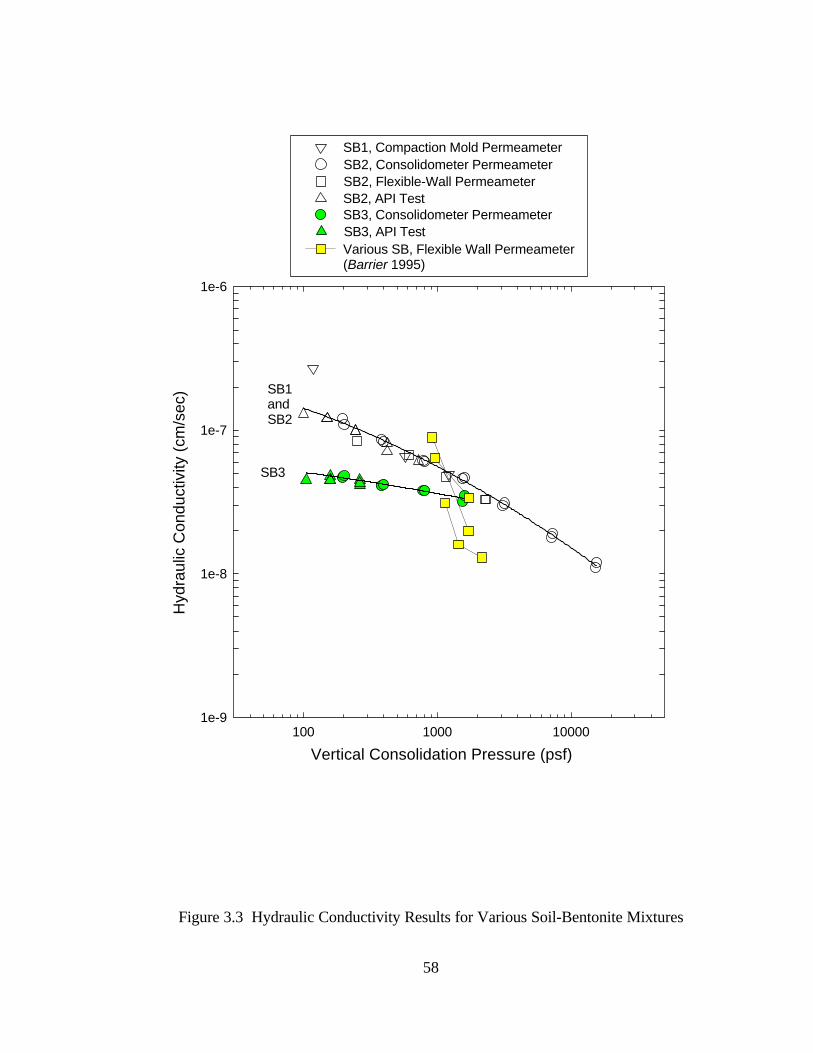
Hydraulic conductivity tests were conducted on soil-bentonite mixtures SB1, SB2, and

SB3. The tests were performed using compaction mold permeameters, consolidometer

permeameters, the API filter press, and flexible-wall permeameters. The results of all the

tests are shown in Figure 3.3. Data from the literature are also plotted in the figure, and

are discussed below.

Experimental Procedures

Three hydraulic conductivity tests were run on SB1 in compaction mold permeameters.

The soil-bentonite was spooned into the mold and rodded to eliminate air voids. The

samples were 4 inches in diameter and the final height was approximately 4 inches.

Surcharge weights were applied to consolidate the soil-bentonite to various effective

stresses. The average vertical effective stress in the sample versus the hydraulic conduc-

tivity is shown in Figure 3.3. The two tests at lower pressure were permeated downward

in falling head tests. In order to achieve the higher pressures for the third test, consider-

able weights were stacked above the top of the compaction mold. The top was left

unassembled and a falling head test was run by permeating upward.

As part of a related research project at Virginia Tech (Heslin et al. 1997), hydraulic

conductivity tests were run on SB2 and SB3 using flexible-wall permeameters, consoli-

dometer permeameters, and the API filter press. The following tests were run on SB2:

One flexible-wall permeability test, two consolidation permeameter tests, and two API

filter press tests. Two consolidation permeameter tests and three API filter press tests

were run on SB3. For each test, the hydraulic conductivity was found at three to seven

different pressures.

36

The flexible-wall test was run using the falling headwater - rising tailwater method de-

scribed in ASTM D-5048 without backpressure. Samples were 2.8 inches in diameter and

3.3 inches in height prior to testing. A forming jacket was used to support the sample

before application of the cell pressure. The forming jacket was left in place during the

test. The effective isotropic consolidation pressure is plotted versus the hydraulic con-

ductivity in Figure 3.3.

Standard incremental load tests were run in the consolidometer permeameter without

backpressure, as described below in Section 3.4. Samples were 2.5 inches in diameter and

1 inch in height. Falling head test hydraulic conductivity tests were conducted after the

end of primary consolidation. The vertical effective consolidation pressure is plotted

versus the hydraulic conductivity in Figure 3.3.

The API filter press is an apparatus commonly used to measure the filtrate loss of slurry.

It has also been used to measure the hydraulic conductivity of soil-bentonite during soil-

bentonite mix design and for QA/QC (Barvenik and Ayers 1987). The API filter press is a

rigid wall cell 3 inches in diameter. Air pressure is applied to the top of the specimen. A

more detailed description of the equipment and test procedure for the consolidometer

permeameter and API filter press test is given in Heslin et al. (1997). A surcharge was

used inside the API cell since it was found that hydraulic fracture occurs in tests without

surcharge. In some of the API filter press tests at the higher pressures, it is believed that

problems occurred with either migration of fines or washing of fines out of the specimen.

These hydraulic conductivity measurements are not included in Figure 3.3.

As described in Heslin et al. (1997), running a hydraulic conductivity test in the API filter

press results in a soil-bentonite specimen that has zero vertical effective stress at the top of

the specimen and a maximum value of vertical effective stress at the bottom of the speci-

37

men. In order to properly interpret the results, the method described by Heslin et al.

(1997) was used to estimate the apparent pressure that should be associated with the

measured gross hydraulic conductivity. This method uses the seepage consolidation

theory by Fox and Baxter (1997), and applies the theory to analysis of hydraulic conduc-

tivity tests in the API filter press. For all of the API tests, the apparent pressure is plotted

versus the gross hydraulic conductivity in Figure 3.3.

Results

The results in Figure 3.3 show that the four different permeameter types all give similar

results. Especially consistent results were found for the consolidometer permeameter,

flexible-wall permeameter, and API test. Less consistent results were found for the

compaction mold permeameter.

Essentially the same hydraulic conductivity was measured for SB1 and SB2. The soil-

bentonite mixtures SB1 and SB2 are identical except that SB1 was created and permeated

with distilled water and SB2 was created and permeated with tap water. SB2 was created

because distilled water is not recommended for permeability testing (Daniel 1994; Dunn

and Mitchell 1984). The results show that for this soil-bentonite mixture, the effect of

using distilled water versus tap water for hydraulic conductivity testing is not significant.

For all of the soil-bentonite mixtures, the hydraulic conductivity decreases with increasing

vertical consolidation pressure. The hydraulic conductivity for SB2 decreases from

approximately 1x10-7 cm/sec at 100 psf to 5x10-8 cm/sec at 1000 psf. The hydraulic

conductivity for SB3 decreases only slightly with increases in consolidation pressure. The

hydraulic conductivity for SB3 is approximately 5x10-8 cm/sec at 100 psf and 3x10-8

cm/sec at 1500 psf. SB3 has a lower hydraulic conductivity than SB2 at all consolidation

pressures. The percentage of bentonite appears to have a larger influence on hydraulic

conductivity than fines content since SB3 has 16% non-plastic fines and 3% bentonite and

38

SB1 has 35% plastic fines and 1% bentonite. SB2 and SB3 both have hydraulic conduc-

tivity values in the range of typically desired soil-bentonite mixtures.

Also plotted in Figure 3.3 is data from Barrier (1995) that was obtained from several

other soil-bentonite mixtures. The data from Barrier (1995) includes results from

McCandless and Bodocsi (1988) and Day (unpublished). As discussed previously in

Section 2.4, the horizontal hydraulic conductivity data from McCandless and Bodocsi

(1988) was measured under a combined vertical surcharge and horizontal hydraulic

pressure. It appears that this data was misinterpreted in Barrier (1995) and is therefore

not included in Figure 3.3. The hydraulic conductivity values of SB2 and SB3 appear to

be in the same range and show similar trends as the Barrier data from Day, although the

data from Day exhibits a greater sensitivity to vertical consolidation pressure.

3.4 Consolidation Tests

Two 1-D consolidation tests and two isotropic consolidation tests were performed on

SB1. Two 1-D consolidation tests were performed on SB3.

The two 1-D consolidation tests on SB1 (C5 and C6) were standard incremental load tests

performed in accordance with ASTM D-2435. The samples were 2.5 inches in diameter

and 1 inch in height. The soil-bentonite was spooned into the consolidation ring and

rodded to eliminate large air voids. Loads were added through a dead weight hanger

system using a load increment ratio of 1 (doubling of the load), and a load increment

duration of 24 hours. Back pressure was not used. The data was corrected for machine

deflection that was estimated using a steel sample. In order to obtain the appropriate

machine deflection curve, it was found that the filter paper needed considerable time to

consolidate under each load (approximately 4 hours). The void ratio versus vertical

effective stress for the two tests are plotted in Figure 3.4 and Figure 3.5. The coefficient

of consolidation, Cv, was calculated for primary loading using the Casagrande method and

39

the Taylor method. The values of Cv are plotted versus the average pressure for each

stress increment.

A trend in the time deformation data for SB1 can be seen from Figures 3.4 and 3.5. As

the effective stress increases, the value of the coefficient of consolidation, Cv, increases

considerably. Cv is defined in equation 3.1, and increases from approximately 5 ft2/yr at

100 psf to 80 ft2/yr at 10,000 psf. Cv is a function of the compressibility and permeability

of the soil-bentonite, which are both decreasing as the effective stress increases. There-

fore, it appears that the compressibility is decreasing at a faster rate than the permeability.

wv

ov a

)e1(kC

γ+

= (3.1)

where: k = hydraulic conductivity

eo = initial void ratio

γw = unit weight of water

av = coefficient of compressibility

The Cv values for SB1 can be compared to typical values for clays. Correlations of Cv

with liquid limit (Holtz and Kovacs 1981) indicate that a typical remolded clay with the

same liquid limit as SB1 (LL=34), would have a Cv value less than or equal to 32 ft2/yr.

Three soil-bentonite mixtures presented by Khoury et al. (1992) had Cv values ranging

from 70 to 292 ft2/yr for the stress range of 2000-4000 psf. For this stress range, SB1 has

a Cv of approximately 40 ft2/yr. The coefficient of consolidation for SB1 is slightly higher

than for a clay with similar liquid limit, but significantly less than the values for soil-

bentonite mixtures reported by Khoury et al. (1992).

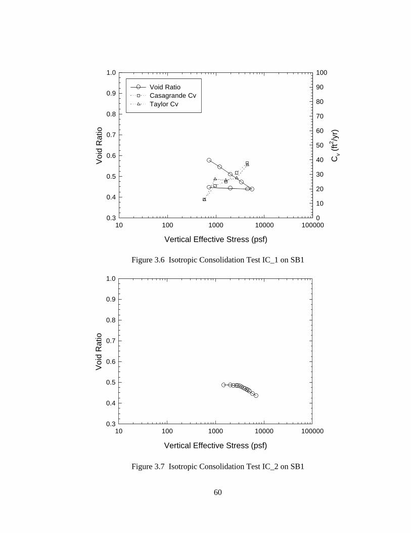
Two isotropic consolidation tests on SB1 (IC-1 and IC-2) were conducted in a triaxial cell

on 2.8 inch diameter samples. The initial height of the samples was approximately 5.6

inches. Special procedures that were developed for triaxial compression testing of soil-

40

bentonite were also used to prepare the isotropic consolidation tests. The soil-bentonite

was spooned into a forming jacket and rodded to eliminate large air voids. The samples

were consolidated inside the forming jacket to an initial pressure of at least 3 psi. It was

found that a 3 psi consolidation pressure was required for the soil-bentonite to be able to

maintain its shape without the forming jacket. After the sample was fully consolidated to

the initial pressure, the triaxial cell was disassembled and the forming jacket was removed.

The sample dimensions were measured at this time. The cell was then reassembled and

the sample was backpressure saturated in small increments in order to avoid overconsoli-

dating the sample. A B-value of 0.99 was reached. Next, the sample was consolidated to

a final pressure to eliminate disturbance effects from the process of removing the forming

jacket.

The sample used for isotropic consolidation test IC_1 was initially consolidated to 3 psi

and finally consolidated to 5 psi. The sample was then loaded using a load increment ratio

of 2/3 and a load increment duration of approximately 48 hours. The sample for isotropic

consolidation test IC_2 was initially consolidated to 10 psi and finally consolidated to 20.3

psi. It was then unloaded to 10 psi and reloaded in increments of 2 psi in order to find the

isotropic yield point. The void ratio versus vertical effective stress curves for IC_1 and

IC_2 are shown in Figure 3.6 and Figure 3.7.

Two 1-D consolidation tests were conducted on specimens of SB3 (CP5 and CP6) in the

consolidometer permeameter cells described in Section 3.3 of this report. The void ratio

versus vertical effective stress curves for the two tests are shown in Figure 3.8 and Figure

3.9. Falling head hydraulic conductivity tests were run at various consolidation pressures

in these tests. The results of the hydraulic conductivity tests are described in Section 3.3.

The results of all the consolidation tests are summarized in Table 3.2. Values of the

compression index Cc and the compression ratio are listed. The compression ratio was

41

calculated for the stress increment between 1000 psf and 4000 psf. The void ratio, e, at

1000 psf was used to calculate the compression ratio. Values of the recompression index,

Cr, are listed together with the preconsolidation pressures, σp’, at the time of rebound.

Holtz and Kovacs (1981) report that the range of compression index for a typical normally

consolidated medium-sensitive clay is 0.2 to 0.5. The average 1-D compression index for

SB1 is 0.19, which is just outside the lower bound of this range. The average isotropic

compression index for SB1 is 0.15, which is also below this range. The average compres-

sion index for SB3 is 0.088, which is approximately 2 times smaller than the value for

SB1. It seems reasonable that SB1 and SB3 are less compressible than a medium sensitive

clay since SB1 is a clayey sand (SC) and SB3 is a silty sand (SM).

Table 3.2 Consolidation Test Results on SB1 and SB3

TestNumber


TestType

Initialw%

eat 1000

psf

Cc CompressionRatio

Cr at σp’ (psf)

C5 SB1 1-D 30.3 0.631 0.18 0.11 0.010 at 4200 psfC6 SB1 1-D 31.7 0.614 0.20 0.12 0.0074 at 1100 psf

0.0095 at 8400 psfIC_1 SB1 isotropic 23.5 0.560 0.16 0.10 0.011 at 5600 psfIC_2 SB1 isotropic 31.9 NA 0.14 NA 0.013 at 2900 psfCP5 SB3 1-D 28.9 0.594 0.082 0.051 0.0029 at 1600 psfCP6 SB3 1-D 28.9 0.595 0.094 0.059 0.0027 at 1600 psf

Notes: The compression ratio was calculated for the stress increment between 1000 psfand 4000 psf.The void ratio at 1000 psf was used to calculate the compression ratio.

The 1-D and isotropic compression ratios for SB1 are both about 0.11. The compression

ratios were evaluated at the same stress increment as the data shown in Figure 2.2 (from

D’Appolonia 1980) in order to compare them. The compression ratios for SB1 are

approximately 1.7 times greater than the compression ratios reported by D’Appolonia for

soil-bentonite mixtures with 35% plastic fines. However, the compression ratios for SB1

are in reasonable agreement with those of Khoury et al. (1992) shown in Table 2.1 and

42

Evans and Cooley (1993) shown in Table 2.2. The average compression ratio for SB3 is

0.056. This value is approximately 2.7 times greater than that reported data by

D’Appolonia for soil-bentonite mixes with 16% non-plastic fines, and it is smaller than the

values in Tables 2.1 and 2.2.

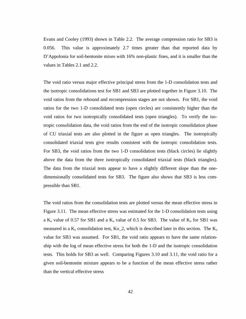
The void ratio versus major effective principal stress from the 1-D consolidation tests and

the isotropic consolidations test for SB1 and SB3 are plotted together in Figure 3.10. The

void ratios from the rebound and recompression stages are not shown. For SB1, the void

ratios for the two 1-D consolidated tests (open circles) are consistently higher than the

void ratios for two isotropically consolidated tests (open triangles). To verify the iso-

tropic consolidation data, the void ratios from the end of the isotropic consolidation phase

of CU triaxial tests are also plotted in the figure as open triangles. The isotropically

consolidated triaxial tests give results consistent with the isotropic consolidation tests.

For SB3, the void ratios from the two 1-D consolidation tests (black circles) lie slightly

above the data from the three isotropically consolidated triaxial tests (black triangles).

The data from the triaxial tests appear to have a slightly different slope than the one-

dimensionally consolidated tests for SB3. The figure also shows that SB3 is less com-

pressible than SB1.

The void ratios from the consolidation tests are plotted versus the mean effective stress in

Figure 3.11. The mean effective stress was estimated for the 1-D consolidation tests using

a Ko value of 0.57 for SB1 and a Ko value of 0.5 for SB3. The value of Ko for SB1 was

measured in a Ko consolidation test, Ko_2, which is described later in this section. The Ko

value for SB3 was assumed. For SB1, the void ratio appears to have the same relation-

ship with the log of mean effective stress for both the 1-D and the isotropic consolidation

tests. This holds for SB3 as well. Comparing Figures 3.10 and 3.11, the void ratio for a

given soil-bentonite mixture appears to be a function of the mean effective stress rather

than the vertical effective stress

43

3.5 Triaxial Tests

The following triaxial tests were run on SB1: Seven isotropically consolidated undrained

triaxial compression tests (CU), one Ko consolidated undrained triaxial compression test,

and nine isotropically consolidated drained triaxial compression tests (CD). The following

triaxial tests were run on SB3: three CU tests, and two CD tests.

Experimental Procedures

2.8 inch diameter triaxial samples, formed with the largest triaxial equipment that was

readily available, were used for testing the soil-bentonite. ASTM D4767 for CU tests

recommends the sample diameter should be at least 6 times greater than the largest

particle size. With the 2.8 inch diameter sample, the largest recommended particle size is

approximately 0.5 inch. The maximum grain size for SB1 and SB3 was limited to passing

the No. 4 sieve (0.2 inches), so the particle size criterion was satisfied. The initial height

of the samples was approximately 5.6 inches.

Due to the soft nature of the soil-bentonite, a new method for forming the sample was

developed. As previously described for the isotropic consolidation tests, samples were

formed inside the triaxial cell in a forming mold (membrane expander). This method was

chosen over consolidation in a batch consolidometer, which would have required higher

pressures in order to extrude and trim the samples. The forming mold provided the least

disturbance and allowed the samples to be formed at the lowest pressures. The samples

were isotropically consolidated inside the forming mold to a pressure of 3 psi or greater.

It was found that 3 psi isotropic pressure for this initial consolidation phase was necessary

for the sample to maintain its shape. A special top cap was machined to slide inside the

forming mold as the sample consolidated. No back pressure was used during the initial

consolidation. The volume of water expelled was measured with a graduated cylinder.

After the sample reached the end of primary consolidation at the initial pressure, the cell

was disassembled. Drainage from the sample was prevented during cell disassembly. The

44

forming mold was removed and the sample dimensions were measured. The cell was then

reassembled without the mold and the sample was backpressure saturated. After a B

value above 0.97 was reached, the sample was consolidated to its final consolidation

pressure. The final consolidation pressure was at least 1.5 times the initial consolidation

pressure in order to minimize disturbance effects from the disassembly process.

After the final consolidation phase, the sample was sheared undrained (CU test) or drained

(CD test). The samples were loaded at a constant strain rate. It is recommended that for

CU tests, the time to failure should be five times t50 for pore pressure equalization

throughout the sample (Brandon 1995), where t50=time to 50% consolidation from the

consolidation stage. For CD tests, time to failure should be 15 to 20 times t50 for pore

pressure dissipation (Brandon 1995). For CU tests, it was decided to use a time to failure

between five to seven times t50. The strain to failure was estimated at 10% axial strain.

Strain rates were typically 2x10-4 to 3x10-4 inch/min or 3x10-3 to 6x10-3 %/min. For CD

tests, 15 to 20 times t50 was used for time to failure. The strain at failure was estimated as

15%. Strain rates were typically 1x10-4 to 2x10-4 inch/min or 2x10-3 to 3x10-3 %/min.

Data acquisition was used to measure the load, effective stress or volume change, and

axial deformation. The data acquisition was always verified with data taken by hand.

Area and Membrane Corrections

Several corrections were made to the data, which are described in more detail in Appendix

A. An area correction was applied, which assumes that the sample deforms as a right

circular cylinder. This correction is recommended by La Rochelle et al. (1988) for speci-

mens exhibiting a bulging type failure, which occurred for all of the triaxial tests per-

formed on soil-bentonite mixtures. After reviewing the literature on membrane correc-

tions, a new membrane correction procedure was developed. The membrane corrections

were based on the compression shell theory by Henkel and Gilbert (1952) with aspects of

other membrane corrections in the literature (Duncan and Seed 1967; La Rochelle et al.

45

1988). The theory was extended to correct for the axial and radial stress on the sample

during the consolidation phase. The correction during the consolidation phase was

important for soil-bentonite testing due to the large strains that occurred during the

consolidation phase. This correction resulted in a very slight anisotropic stress state at the

end of the supposedly isotropic consolidation phase. The major effective stress after

consolidation was in the radial direction. The difference in the major and minor effective

principal stresses was 0.2 psi for low consolidation pressures (5 psi) and 0.8 psi for the

largest consolidation pressure (39 psi). During the shearing phase, the membrane correc-

tion described in ASTM D4767 was applied to the axial stress. The modulus of the

membrane used in the membrane corrections was the initial tangent modulus, which was

measured experimentally. Piston friction in the triaxial cell was assumed to be constant

and was zeroed out at the start of the test.

Isotropically Consolidated Undrained Triaxial Tests

Seven isotropically consolidated undrained triaxial tests (CU) were run on SB1 (CU_3

through CU_9). Two of the samples were used for isotropic consolidation tests before

being sheared. Isotropic consolidation test IC_1 was sheared as CU_8 and IC_2 was

sheared as CU_9. All of the samples were sheared essentially normally consolidated

except for CU_8, which was sheared slightly overconsolidated. The data from the first

two tests CU_1 and CU_2 was not of good quality and was not used. Several problems

with data acquisition were solved and procedures were refined during the first two tests.

During undrained tests, it was found that pore pressures would build up in the sample after

primary consolidation was complete and the drainage valve was closed to begin shearing.

It is thought that the pore pressure build up was due to the phenomenon referred to as

“undrained creep” by Head (1986). After the valve was closed, the piston had to travel

into a seating groove in the top cap before making contact with the sample. Due to the

very slow strain rates that were used, the drainage valve was often closed for a significant

46

time (up to 4 hours) before the piston made contact with the sample. The maximum pore

pressure that developed during this time period due to undrained creep was approximately

2.7 psi. On average, the pore pressure in the sample at contact was about 1 psi.

In subsequent figures, the triaxial compression results are plotted as stress paths using

both the MIT convention and the critical state convention. The variables p’ and q, ac-

cording to these conventions, are defined below:

MIT stress path convention:

p’ = (σ1’ + σ3’)/2 (3.2)

q = (σ1’ - σ3’)/2 (3.3)

Critical state stress path convention:

p’ = (σ1’ + σ2’ + σ3’)/3 (3.4)

q = (σ1’ - σ3’) (3.5)

where: σ1’ = major principal effective stress

σ2’ = intermediate principal effective stress

σ3’ = minor principal effective stress

The MIT convention is commonly used in the United States and is easily related to φ’ and

c’. The critical state convention is commonly used in many constitutive models, such as

the Cam Clay model. The critical state p’ is equal to the mean effective stress. The

critical state q is equal to the deviator stress. The failure line in MIT p-q space is called

the Kf line. The failure line in critical state p-q space is called the M line. The M line is

the projection of the critical state line in p-q space.

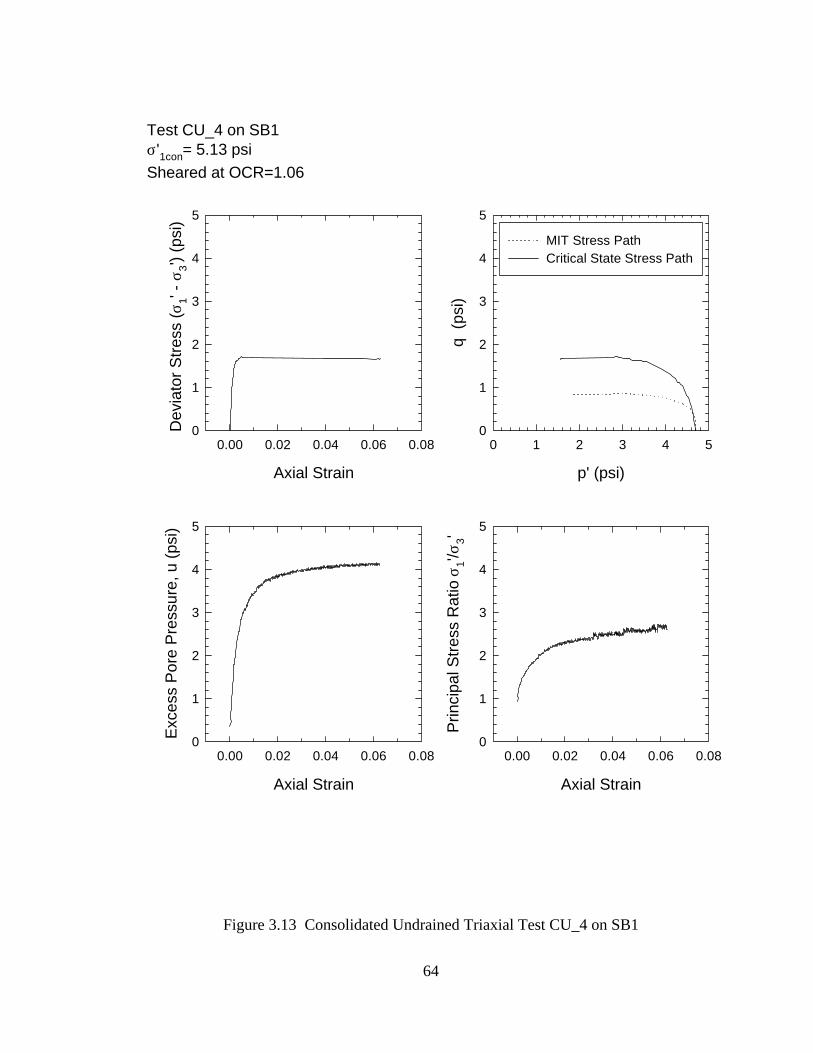
The MIT and critical state stress paths for tests CU_3 through CU_9 are shown in Figure

3.12 through Figure 3.18. The deviator stress, excess pore pressure, and principal stress

ratio (σ1’/σ3’) are also plotted versus axial strain. The excess pore pressure includes the

47

excess pore pressure in the sample present due to undrained creep. Undrained creep

produces an excess pore pressure plotted at zero axial strain.

The maximum principal stress ratio was used as the failure criterion for all of the CU tests.

For a normally consolidated material with a linear failure envelope, the maximum principal

stress ratio develops when the stress path is on the Kf line. In general, the stress paths are

initially steep, then curve to the left and become relatively horizontal. Large excess pore

pressures develop and the stress path either stops at the Kf line or travels up the Kf line.

Most of the shear stress is mobilized at small axial strains.

The results of the CU tests on SB1 are summarized in Table 3.3. For the CU tests, the

overconsolidation ratio (OCR) is the major principal effective stress at the end of consoli-

dation (σ’1con) divided by the major principal effective stress at the start of shear (σ’1shear).

A-bar is defined as the increase in excess pore pressure over increase in deviator stress.

The excess pore pressure that occurs due to undrained creep prior to applying the deviator

stress is not included in the A-bar calculation since it is not associated with the increase in

deviator stress. For the normally consolidated tests, the average axial strain at failure was

6.5%; the average A-bar at failure was 2.0; and the average su/σ’1con was 0.19.

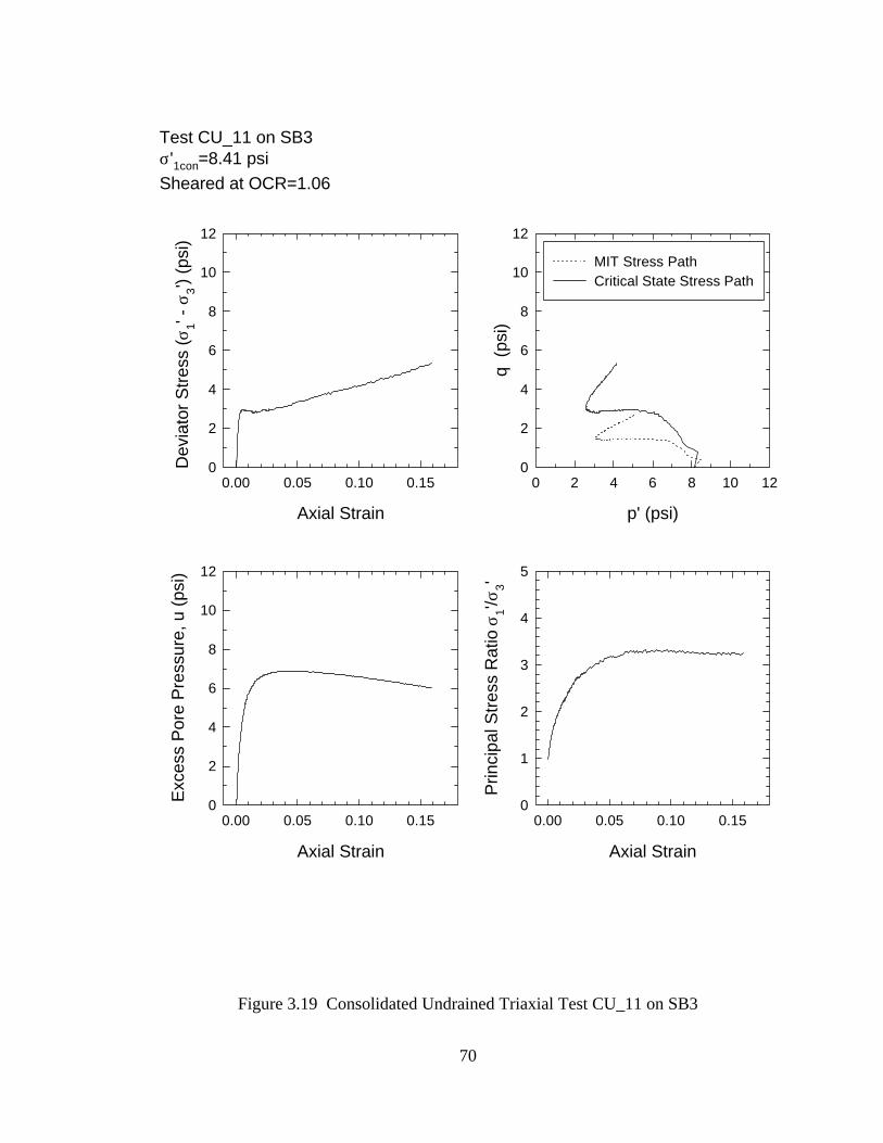
Three CU tests (CU_11, CU_13, CU_14) were run on SB3. All of the samples were

isotropically consolidated and sheared normally consolidated. The tests results are shown

in Figure 3.19 through Figure 3.21. In general, the stress strain curves are initially steep,

slight strain softening occurs until the stress paths hit the Kf line, then the stress paths

travel up the Kf line. Failure is defined at the point when the stress path reaches the Kf

line. The results of CU tests on SB3 are summarized in Table 3.4. For the three tests, the

average OCR is 1.01; the average axial strain to failure is 3.4%; the average A-bar at

failure is 2.2; and the average su/σ’1con is 0.16.

48

Table 3.3 Isotropically Consolidated Undrained Triaxial Test Results for SB1

Test σ’1con

(psi)OCR Water

Content(%)

VoidRatio

Axial Strainat Failure

(%)

A-bar atFailure

su

(psi)su /

σ’1con

CU_3 18.43 1.09 18.2 0.49 7.2 2.0 3.78 0.21CU_4 5.13 1.06 22.0 0.60 6.3 2.1 0.83 0.16CU_5 8.57 1.03 20.2 0.55 5.2 2.0 1.59 0.19CU_6 5.12 1.09 22.0 0.60 5.0 2.0 0.90 0.18CU_7 12.42 1.08 19.4 0.53 6.0 1.7 2.75 0.22CU_8 39.1 1.32 16.2 0.44 7.5 1.5 7.70 0.20CU_9 48.18 1.06 16.1 0.44 9.1 2.0 9.21 0.19avg. of3-7,9 NA 1.07 NA NA 6.5 2.0 NA 0.19

Notes: σ’1con = major principal effective stress at the end of consolidationσ’1shear = major principal effective stress at the beginning of shearOCR = σ’1con/σ’1shear

A-bar = change in excess pore pressure / change in deviator stresssu = undrained shear strength, defined at maximum principal stress

ratioWater content and void ratio given at the end of consolidation

Table 3.4 Isotropically Consolidated Undrained Triaxial Test Results for SB3

Test σ’1con

(psi)OCR Water

Content(%)

VoidRatio

Axial Strainat Failure

(%)

A-bar atFailure

su

(psi)su /

σ’1con

CU_11 8.41 1.00 21.6 0.57 2.4 2.2 1.46 0.17CU_13 12.48 1.04 20.7 0.55 2.9 2.6 1.76 0.14CU_14 20.36 1.00 19.8 0.52 4.9 2.3 3.5 0.17avg. NA 1.01 NA NA 3.4 2.4 NA 0.16

Notes: σ’1con = major principal effective stress at the end of consolidationσ’1shear = major principal effective stress at the beginning of shearOCR = σ’1con/σ’1shear

A-bar = change in excess pore pressure / change in deviator stresssu = undrained shear strength, defined at maximum principal stress

ratioWater content and void ratio are reported at the end of consolidation

49

Ko Consolidated Undrained Triaxial Test

One Ko consolidation test (Ko_2) was run on SB1. The burette method described by Al-

Hussaini (1981) was used. Al-Hussaini (1981) presents the results of four different

methods of measuring Ko for sands in triaxial cells. The methods are 1) LVDT clamp

with lateral strain sensor 2) strain gauge Ko belt 3) swinging arms lateral strain sensor

and 4) burette method. Since the author concludes that all the tests give similar results,

the burette method was used for test Ko_2 since it is the simplest method. The method

involves monitoring the axial and volumetric strain and adjusting the cell pressure to

maintain a Ko condition.

A stress path for the Ko consolidation and subsequent undrained shearing is shown in

Figure 3.22. This figure illustrates the various stages of the test. A 2.8 inch diameter

sample was prepared in a triaxial cell with initial specimen height of approximately 5.6

inches. The soil-bentonite was spooned inside a forming mold in the triaxial cell and first

isotropically consolidated to 4 psi to point A inside the mold. After the 4 psi consolida-

tion, it was decided to consolidate to a higher isotropic consolidation pressure of 16 psi to

point B in order to take advantage of the higher coefficient of consolidation values exhib-

ited at higher pressures in the consolidation tests. After final isotropic consolidation, the

mold was left on and a deviator stress was applied in drained loading to bring the sample

to an estimated value of Ko=0.5 at point C. Back pressure was not used in these stages

and the volume of water expelled was measured with a graduated cylinder. After the

sample had reached the estimated Ko state at point C, the sample was unloaded fully to

point O. Next the drainage was closed on the specimen, the cell was disassembled, the

forming mold was removed, and the sample dimensions were measured. The sample was

reconsolidated to 4 psi to point A and backpressure saturated. A B-value of 0.95 was

reached. The sample was then reconsolidated to 16 psi. A deviator stress was then

applied in drained loading to bring the sample back to point C on the estimated Ko line.

50

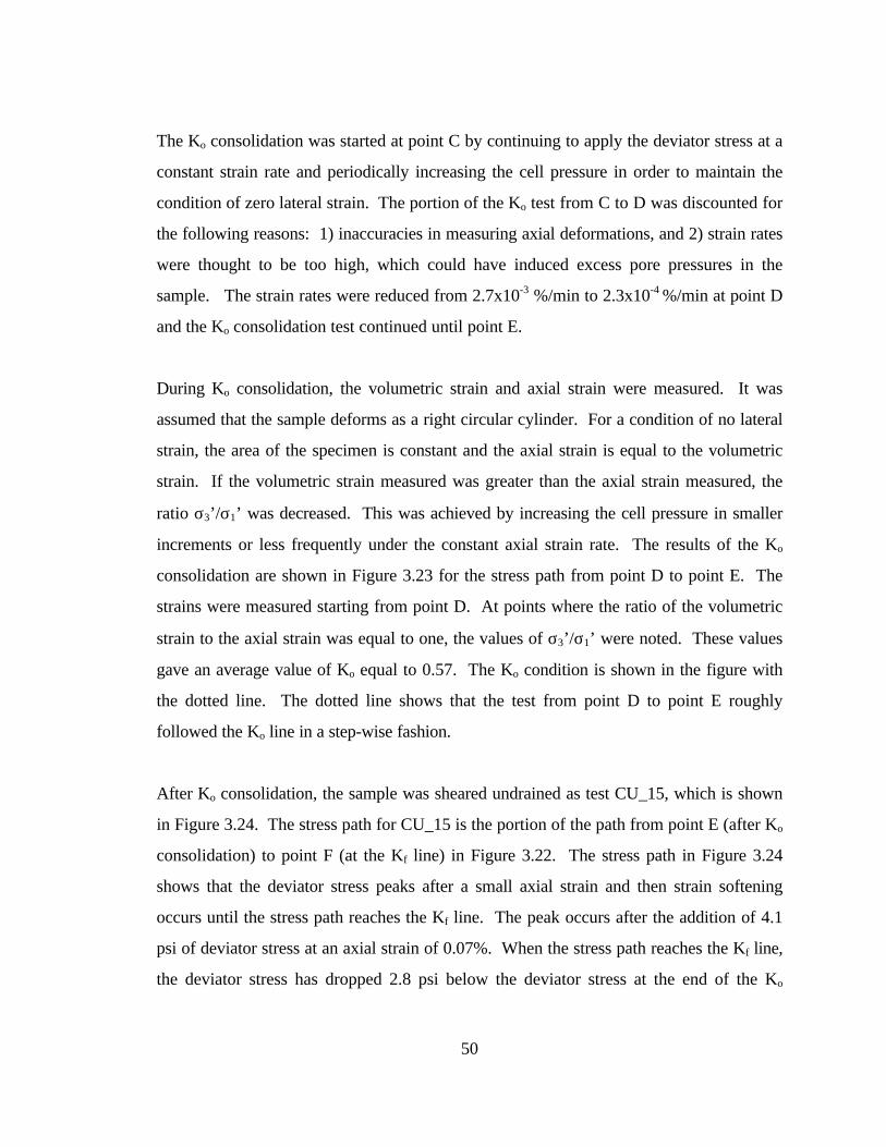
The Ko consolidation was started at point C by continuing to apply the deviator stress at a

constant strain rate and periodically increasing the cell pressure in order to maintain the

condition of zero lateral strain. The portion of the Ko test from C to D was discounted for

the following reasons: 1) inaccuracies in measuring axial deformations, and 2) strain rates

were thought to be too high, which could have induced excess pore pressures in the

sample. The strain rates were reduced from 2.7x10-3 %/min to 2.3x10-4 %/min at point D

and the Ko consolidation test continued until point E.

During Ko consolidation, the volumetric strain and axial strain were measured. It was

assumed that the sample deforms as a right circular cylinder. For a condition of no lateral

strain, the area of the specimen is constant and the axial strain is equal to the volumetric

strain. If the volumetric strain measured was greater than the axial strain measured, the

ratio σ3’/σ1’ was decreased. This was achieved by increasing the cell pressure in smaller

increments or less frequently under the constant axial strain rate. The results of the Ko

consolidation are shown in Figure 3.23 for the stress path from point D to point E. The

strains were measured starting from point D. At points where the ratio of the volumetric

strain to the axial strain was equal to one, the values of σ3’/σ1’ were noted. These values

gave an average value of Ko equal to 0.57. The Ko condition is shown in the figure with

the dotted line. The dotted line shows that the test from point D to point E roughly

followed the Ko line in a step-wise fashion.

After Ko consolidation, the sample was sheared undrained as test CU_15, which is shown

in Figure 3.24. The stress path for CU_15 is the portion of the path from point E (after Ko

consolidation) to point F (at the Kf line) in Figure 3.22. The stress path in Figure 3.24

shows that the deviator stress peaks after a small axial strain and then strain softening

occurs until the stress path reaches the Kf line. The peak occurs after the addition of 4.1

psi of deviator stress at an axial strain of 0.07%. When the stress path reaches the Kf line,

the deviator stress has dropped 2.8 psi below the deviator stress at the end of the Ko

51

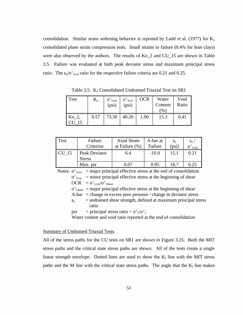
consolidation. Similar strain softening behavior is reported by Ladd et al. (1977) for Ko

consolidated plane strain compression tests. Small strains to failure (0.4% for lean clays)

were also observed by the authors. The results of Ko_2 and CU_15 are shown in Table

3.5. Failure was evaluated at both peak deviator stress and maximum principal stress

ratio. The su/σ’1con ratio for the respective failure criteria are 0.21 and 0.25.

Table 3.5. Ko Consolidated Undrained Triaxial Test on SB1

Test Κο σ’1con

(psi)σ’3con

(psi)OCR Water

Content(%)

VoidRatio

Ko_2,CU_15

0.57 73.50 40.20 1.00 15.3 0.41

Test FailureCriterion

Axial Strainat Failure (%)

A-bar atFailure

su

(psi)su /

σ’1con

CU_15 Peak DeviatorStress

6.4 -10.0 15.1 0.21

Max. psr 0.07 0.95 18.7 0.25Notes: σ’1con = major principal effective stress at the end of consolidation

σ’3con = minor principal effective stress at the beginning of shearOCR = σ’1con/σ’1shear

σ’1shear = major principal effective stress at the beginning of shearA-bar = change in excess pore pressure / change in deviator stresssu = undrained shear strength, defined at maximum principal stress

ratiopsr = principal stress ratio = σ’1/σ’3

Water content and void ratio reported at the end of consolidation

Summary of Undrained Triaxial Tests

All of the stress paths for the CU tests on SB1 are shown in Figure 3.25. Both the MIT

stress paths and the critical state stress paths are shown. All of the tests create a single

linear strength envelope. Dotted lines are used to show the Kf line with the MIT stress

paths and the M line with the critical state stress paths. The angle that the Kf line makes

52

with the horizontal is called alpha, α’, and the intercept is called d’. These variables can

be related to φ’ and c’ by the following equations:

'sin'tan φ=α (3.6)

'cos

'd'c

φ= (3.7)

The slope of the M line is the critical state parameter M. For the case of triaxial compres-

sion, M is related to φ’ by the following equation (Wood 1990):

'sin3

'sin6M

φ−φ

= (3.8)

All of the stress paths for the CU tests on SB3 are shown in Figure 3.26. Again, the tests

create a single linear strength envelope. The strength envelope for SB3 is the same as for

SB1. The resulting undrained strength parameter values for SB1 and SB3 are listed in

Table 3.6.

Table 3.6 Undrained Strength Parameter Values for SB1 and SB3


φ’(degrees)

c’(psi)

α’(degrees)

d’(psi)

M

SB1 32 0 28 0 1.3SB3 32 0 28 0 1.3

Isotropically Consolidated Drained Triaxial Tests

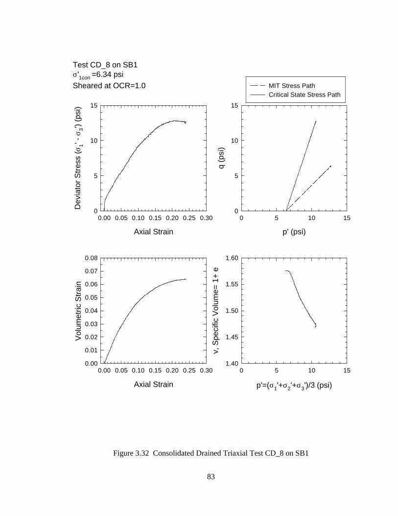
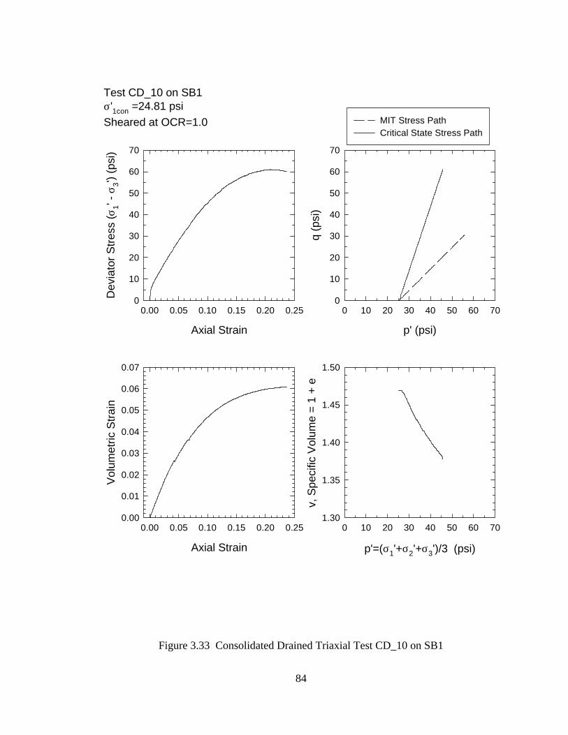
Nine isotropically consolidated drained triaxial tests (CD_1 through CD_8 and CD_10)

were performed on SB1. Two CD tests (CD_11 and CD_12) were run on SB3. The tests

on SB1 were designed to determine constitutive model parameters. Tests CD_1, CD_8,

and CD_10 were run on isotropically consolidated samples which were sheared normally

consolidated to failure to find the strength envelope and the parameter values for the

hyperbolic model described by Duncan and Chang (1970). Tests CD_2 through CD_7

were sheared overconsolidated in order to gain information on the yield surface and plastic

53

potential surface. All of these tests were isotropically consolidated to 20 psi, then re-

bounded isotropically to various overconsolidation ratios. A few of these tests were not

run to failure (CD_3 and CD_4). The tests on SB3 were run on isotropically consolidated

samples that were sheared to failure. Except for tests CD_3 and CD_4, the test results are

presented in this chapter. Interpretation of the tests to determine constitutive model

parameters is discussed in Chapter 4.

The test results for SB1 are shown in Figure 3.27 through Figure 3.33. Tests CD_3 and

CD_4 are not shown since they were not run to failure. The MIT and critical state stress

paths are shown in the figures. The deviator stress and volumetric strain are plotted

versus axial strain. The specific volume is plotted versus mean effective stress. The

specific volume is defined as 1 plus the void ratio. It is a convenient parameter that is

commonly used in critical state models (Wood 1990).

For a CD test, since σ'3 is constant, the MIT stress path rises at a 1 on 1 slope and the

critical state stress path rises at a 3 on 1 slope (Wood 1990). From Figure 3.27, it can be

seen that the stress path for test CD_1 rises in a slightly crooked fashion. This is due to

varying levels of pore water in the outflow burette. In subsequent tests, the burette was

emptied frequently to keep the water in the outflow burette fairly constant.

The normally consolidated tests (CD_1, CD_8, CD_10) have gradually sloping stress

strain curves. The overconsolidated tests have initially steep stress strain curves. A

change in compressibility after yield in the overconsolidated samples can be seen from the

specific volume plots. A negative volumetric strain value signifies volumetric expansion

or dilation. All samples are contractive except for the most overconsolidated samples

CD_6 and CD_7. Both CD_6 and CD_7 initially contract and then dilate. A summary of

the CD tests performed on SB1 is given in Table 3.7.

54

Table 3.7 Isotropically Consolidated Drained Triaxial Test Results for SB1

Test σ’1con

(psi)OCR atStart ofShear

σ’3 atFailure(psi)


AxialStrain atFailure

(%)

WaterContent at

Failure(%)

VoidRatio atFailure

CD_1 14.33 1.0 14.28 46.49 19.8 15.16 0.411CD_2 20.47 3.1 6.71 21.29 16.7 16.43 0.445CD_3 20.48 1.4 14.56 NA NA NA NACD_4 20.46 1.1 18.56 NA NA NA NACD_5 20.36 1.9 10.54 35.12 21.7 15.93 0.432CD_6 20.52 7.8 2.63 8.88 6.75 18.80 0.510CD_7 20.48 8.0 2.56 9.43 11.4 18.46 0.500CD_8 6.34 1.0 6.34 19.19 21.1 17.32 0.469CD_10 25.38 1.0 25.38 86.06 19.7 13.94 0.378

Notes: σ’1con = major principal effective stress at the end of consolidationOCR = σ’1con/σ’1shear

σ’1shear = major principal effective stress at the beginning of shear

Two CD tests (CD_11 and CD_12) were run on SB3. The samples were isotropically

consolidated and sheared normally consolidated. The test results are shown in Figure 3.34

and Figure 3.35. The deviator stress versus axial strain plots look similar to CD tests on

normally consolidated samples of SB1. Both SB3 samples reach a maximum deviator

stress at approximately 17% axial strain. Both samples are initially contractive, and then

exhibit dilation at approximately 11%. Dilation was not measured in normally consoli-

dated CD tests on SB1. Under similar confining pressures, SB3 exhibits less volumetric

strain than SB1. SB3 was also shown to be less compressible than SB1 in 1-D consolida-

tion tests. A summary of the CD tests performed on SB3 is shown in Table 3.8.

The CD strength envelopes for SB1 and SB3 are shown in Figure 3.36 and Figure 3.37.

Only the tests that were normally consolidated or normally consolidated at failure are

shown. For SB1, the effective friction angle, φ’, is 32 degrees and the cohesion is zero.

For SB3, the effective friction angle, φ’, is 33 degrees, and the cohesion is zero. The

drained strength parameter values are listed in Table 3.9. These friction angles found from

55

the CD tests are within one degree of those found from the CU tests and are consistent

with the range of values found for soil-bentonite in the literature (φ’=31 to 33 degrees).

Table 3.8 Isotropically Consolidated Drained Triaxial Test Results for SB3

Test σ’1con

(psi)OCR atStart ofShear



AxialStrain atFailure

(%)

WaterContent at

Failure(%)

VoidRatio atFailure

CD_11 10.00 1.0 10.28 35.78 16.4 18.79 0.498CD_12 13.31 1.0 13.59 48.50 18.2 18.47 0.489

Notes: σ’1con = major principal effective stress at the end of consolidationOCR = σ’1con/σ’1shear

σ’1shear = major principal effective stress at the beginning of shear

Table 3.9 Drained Strength Parameter Values for SB1 and SB3


φ’(degrees)

c’(psi)

α’(degrees)

d’(psi)

M

SB1 32 0 28 0 1.3SB3 33 0 29 0 1.3

Grain Size (mm)

0.0010.010.1110100

Per

cent

Fin

er b

y W

eigh

t (%

)

0

10

20

30

40

50

60

70

80

90

100

Cobbles andGravel Sand Silt and Clay

SB3

SB1 and SB2

Figure 3.1 Grain Size Distributions of SB1, SB2, and SB3

56

Water Content (%)

0 5 10 15 20 25 30 35 40 45 50

Slu

mp

(inch

)

0

2

4

6

8

10

Figure 3.2 Slump Versus Water Content for Various Soil-Bentonite Mixtures

Legend:

%Gravel %Sand %Fines Source

0 65 35 SB1

3 33 64 D'Appolonia (1980)

20 45 35 D'Appolonia (1980)

0 45 55 D'Appolonia (1980)

12 64 22 D'Appolonia (1980)

57

Vertical Consolidation Pressure (psf)

100 1000 10000

Hyd

raul

ic C

ondu

ctiv

ity (

cm/s

ec)

1e-9

1e-8

1e-7

1e-6

SB3

SB1andSB2

Figure 3.3 Hydraulic Conductivity Results for Various Soil-Bentonite Mixtures

58

SB1, Compaction Mold PermeameterSB2, Consolidometer PermeameterSB2, Flexible-Wall PermeameterSB2, API TestSB3, Consolidometer PermeameterSB3, API TestVarious SB, Flexible Wall Permeameter (Barrier 1995)

Vertical Effective Stress (psf)

10 100 1000 10000 100000

Voi

d R

atio

0.3

0.4

0.5

0.6

0.7

0.8

0.9

1.0

Cv

(ft2 /y

r)

0

10

20

30

40

50

60

70

80

90

100Void RatioCasagrande CvTaylor Cv


10 100 1000 10000 100000

Voi

d R

atio

0.3

0.4

0.5

0.6

0.7

0.8

0.9

1.0

Cv

(ft2 /y

r)

0

10

20

30

40

50

60

70

80

90

100

Void RatioCasagrande CvTaylor Cv

Figure 3.4 One-Dimensional Consolidation Test C5 on SB1

Figure 3.5 One-Dimensional Consolidation Test C6 on SB1

59


10 100 1000 10000 100000

Voi

d R

atio

0.3

0.4

0.5

0.6

0.7

0.8

0.9

1.0

Cv

(ft2 /y

r)

0

10

20

30

40

50

60

70

80

90

100

Void RatioCasagrande CvTaylor Cv


10 100 1000 10000 100000

Voi

d R

atio

0.3

0.4

0.5

0.6

0.7

0.8

0.9

1.0

Figure 3.6 Isotropic Consolidation Test IC_1 on SB1

Figure 3.7 Isotropic Consolidation Test IC_2 on SB1

60


10 100 1000 10000 100000

Voi

d R

atio

0.3

0.4

0.5

0.6

0.7

0.8

0.9

1.0


10 100 1000 10000 100000

Voi

d R

atio

0.3

0.4

0.5

0.6

0.7

0.8

0.9

1.0

Figure 3.8 One-Dimensional Consolidation Test CP5 on SB3

Figure 3.9 One-Dimensional Consolidation Test CP6 on SB3

61

Major Principal Effective Stress (psf)10 100 1000 10000 100000

Voi

d R

atio

0.3

0.4

0.5

0.6

0.7

0.8

0.9

1.0

1-D Consolidation Tests on SB1Isotropic Consolidation Tests on SB1 andIsotropically Consolidated CU Tests on SB1 1-D Consolidation Tests on SB3Isotropic Consolidated CU Tests on SB3

Mean Effective Stress (psf)10 100 1000 10000 100000

Voi

d R

atio

0.3

0.4

0.5

0.6

0.7

0.8

0.9

1.0

1-D Consolidation Tests on SB1Isotropic Consolidation Tests on SB1and Isotropically Consolidated CU Tests on SB11-D Consolidation Tests on SB3Isotropically Consolidated CU Tests on SB3

Figure 3.10 Major Principal Effective Stress Versus Void Ratio for Consolidation Tests on SB1 and SB3

Figure 3.11 Mean Effective Stress Versus Void Ratio for Consolidation Tests on SB1 and SB3

SB1

SB3

SB1

SB3

62

p' (psi)

0 5 10 15 20q

(ps

i)

0

5

10

15

20

MIT Stress PathCritical State Stress Path

Axial Strain

0.00 0.02 0.04 0.06 0.08

Exc

ess

Por

e P

ress

ure,

u (

psi)

0

5

10

15

20

Axial Strain

0.00 0.02 0.04 0.06 0.08

Dev

iato

r S

tres

s (σ

1' -

σ 3') (

psi)

0

5

10

15

20

Axial Strain

0.00 0.02 0.04 0.06 0.08

Prin

cipa

l Str

ess

Rat

io σ

1'/σ 3'

0

1

2

3

4

5

Test CU_3 on SB1σ'1con = 18.43 psiSheared at OCR=1.09

Figure 3.12 Consolidated Undrained Triaxial Test CU_3 on SB1

63

p' (psi)

0 1 2 3 4 5q

(ps

i)

0

1

2

3

4

5


Axial Strain

0.00 0.02 0.04 0.06 0.08

Exc

ess

Por

e P

ress

ure,

u (

psi)

0

1

2

3

4

5

Axial Strain

0.00 0.02 0.04 0.06 0.08

Dev

iato

r S

tres

s (σ

1' -

σ 3') (

psi)

0

1

2

3

4

5

Test CU_4 on SB1σ'1con= 5.13 psiSheared at OCR=1.06

Axial Strain

0.00 0.02 0.04 0.06 0.08

Prin

cipa

l Str

ess

Rat

io σ

1'/σ 3'

0

1

2

3

4

5


64

p' (psi)

0 2 4 6 8 10q

(ps

i)

0

2

4

6

8

10


Axial Strain

0.00 0.02 0.04 0.06 0.08

Exc

ess

Por

e P

ress

ure,

u (

psi)

0

2

4

6

8

10

Axial Strain

0.00 0.02 0.04 0.06 0.08

Dev

iato

r S

tres

s (σ

1' - σ

3') (

psi)

0

2

4

6

8

10

Test CU_5 on SB1σ'1con=8.57 psiSheared at OCR=1.03

Axial Strain

0.00 0.02 0.04 0.06 0.08

Prin

cipa

l Str

ess

Rat

io σ

1'/σ 3'

0

1

2

3

4

5


65

p' (psi)

0 1 2 3 4 5q

(ps

i)

0

1

2

3

4

5


Axial Strain

0.00 0.05 0.10 0.15

Exc

ess

Por

e P

ress

ure,

u (

psi)

0

1

2

3

4

5

Axial Strain

0.00 0.05 0.10 0.15

Dev

iato

r S

tres

s (σ

1' -

σ 3') (

psi)

0

1

2

3

4

5


Axial Strain

0.00 0.05 0.10 0.15

Prin

cipa

l Str

ess

Rat

io σ

1'/σ 3'

0

1

2

3

4

5


66

p' (psi)

0 2 4 6 8 10 12q

(ps

i)

0

2

4

6

8

10

12


Axial Strain

0.00 0.05 0.10 0.15

Exc

ess

Por

e P

ress

ure,

u (

psi)

0

2

4

6

8

10

12

Axial Strain

0.00 0.05 0.10 0.15

Dev

iato

r S

tres

s (σ

1' -

σ 3') (

psi)

0

2

4

6

8

10

12


Axial Strain

0.00 0.05 0.10 0.15

Prin

cipa

l Str

ess

Rat

io σ

1'/σ 3'

0

1

2

3

4

5


67

p' (psi)

0 5 10 15 20 25 30q

(ps

i)

0

5

10

15

20

25

30


Axial Strain

0.00 0.05 0.10 0.15

Exc

ess

Por

e P

ress

ure,

u (

psi)

0

5

10

15

20

25

30

Axial Strain

0.00 0.05 0.10 0.15

Dev

iato

r S

tres

s (σ

1' -

σ 3') (

psi)

0

5

10

15

20

25

30


Axial Strain

0.00 0.05 0.10 0.15

Prin

cipa

l Str

ess

Rat

io σ

1'/σ

3'

0

1

2

3

4

5


68

p' (psi)

0 10 20 30 40 50q

(ps

i)

0

10

20

30

40

50


Axial Strain

0.00 0.05 0.10 0.15 0.20 0.25

Exc

ess

Por

e P

ress

ure,

u (

psi)

0

10

20

30

40

50

Axial Strain

0.00 0.05 0.10 0.15 0.20 0.25

Dev

iato

r S

tres

s (σ

1' -

σ 3') (

psi)

0

10

20

30

40

50

Test CU_9 on SB1σ'1con= 47.78 psiIsotropically Consolidated as IC_2 and Sheared at OCR=1.06 as CU_9

Axial Strain

0.00 0.05 0.10 0.15 0.20 0.25

Prin

cipa

l Str

ess

Rat

io σ

1'/σ 3'

0

1

2

3

4

5


69

p' (psi)

0 2 4 6 8 10 12q

(ps

i)

0

2

4

6

8

10

12


Axial Strain

0.00 0.05 0.10 0.15

Exc

ess

Por

e P

ress

ure,

u (

psi)

0

2

4

6

8

10

12

Axial Strain

0.00 0.05 0.10 0.15

Dev

iato

r S

tres

s (σ

1' -

σ 3') (

psi)

0

2

4

6

8

10

12


Axial Strain

0.00 0.05 0.10 0.15

Prin

cipa

l Str

ess

Rat

io σ

1'/σ 3'

0

1

2

3

4

5


70

p' (psi)

0 2 4 6 8 10 12 14q

(ps

i)

0

2

4

6

8

10

12

14


Axial Strain

0.00 0.05 0.10

Exc

ess

Por

e P

ress

ure,

u (

psi)

0

2

4

6

8

10

12

14

Axial Strain

0.00 0.05 0.10

Dev

iato

r S

tres

s (σ

1' -

σ 3') (

psi)

0

2

4

6

8

10

12

14


Axial Strain

0.00 0.05 0.10

Prin

cipa

l Str

ess

Rat

io σ

1'/σ 3'

0

1

2

3

4

5


71

p' (psi)

0 5 10 15 20 25q

(ps

i)

0

5

10

15

20

25


Axial Strain

0.00 0.05 0.10 0.15

Exc

ess

Por

e P

ress

ure,

u (

psi)

0

5

10

15

20

25

Axial Strain

0.00 0.05 0.10 0.15

Dev

iato

r S

tres

s (σ

1' -

σ 3') (

psi)

0

5

10

15

20

25

Test CU_14 on SB3σ'1con=20.36 psiSheared at OCR = 1.00

Axial Strain

0.00 0.05 0.10 0.15

Prin

cipa

l Str

ess

Rat

io σ

1'/σ 3'

0

1

2

3

4

5


72

Figure 3.22 Combined Stress Path for Ko Consolidation Test Ko_2 on SB1

Subsequently Sheared Undrained as Test CU_15

MIT p'=(σ1'+σ ')/2(psi)

0 10 20 30 40 50 60

MIT

q=

(σ1'-

σ 3')/2

(ps

i)

0

10

20

30

40

50

60

O A B

CD

FE

73

MIT p' = (σ1' + σ3')/2 (psi)

0 10 20 30 40 50 60M

IT q

=(σ

1' -

σ 3')/2

(ps

i)

0

10

20

30

40

50

60

MIT p'=(σ1'+σ3')/2 (psi)

30 35 40 45 50 55 60

σ 3'/σ 1'

0.0

0.1

0.2

0.3

0.4

0.5

0.6

0.7

0.8

0.9

1.0

Axial Strain

0.00 0.01 0.02

σ 3'/σ 1'

0.0

0.1

0.2

0.3

0.4

0.5

0.6

0.7

0.8

0.9

1.0

MIT p'= (σ1'+σ3')/2 (psi)

30 35 40 45 50 55 60

Vol

umet

ric S

trai

n / A

xial

Str

ain

0.0

0.5

1.0

1.5

2.0

Figure 3.23 Ko Consolidation Test Ko_2 on SB1

Ko = 0.57Ko = 0.57

D

E

D

E

D DE E

74

Test CU_15 on SB1σ'1con=73.52 psi, σ'3con=40.21psiKo Consolidated as Ko_2 and Sheared at OCR=1.00 as CU_15

MIT p'=(σ1'+σ3')/2(psi)

0 10 20 30 40 50 60M

IT q

=(σ

1'-σ 3')

/2 (

psi)

0

10

20

30

40

50

60

Axial Strain

0.00 0.05 0.10 0.15 0.20

MIT

q=

(σ1'-

σ 3')/2

(ps

i)

0

10

20

30

40

50

60

Axial Strain

0.00 0.05 0.10 0.15 0.20

Exc

ess

Por

e P

ress

ure,

u (

psi)

0

10

20

30

40

50

60

Axial Strain

0.00 0.05 0.10 0.15 0.20

Prin

cipa

l Str

ess

Rat

io (σ

3'/σ 1')

0

1

2

3

4

5

End of Ko Consolidation

Figure 3.24 Ko Consolidated Undrained Triaxial Test CU_15 on SB1

FE

75

p' = (σ1' + σ3') / 2 (psi)

0 10 20 30 40 50 60

q =

(σ 1'

- σ 3')

/ 2

(psi

)

0

10

20

30

40

50

60

MIT Stress Paths

α'=28d'=0φ'=32c'=0

p'=(σ1'+σ2'+σ3')/3 (psi)

0 10 20 30 40 50 60

q=(σ

1'-σ 3')

(ps

i)

0

10

20

30

40

50

60

CU_3CU_4CU_5CU_6CU_7IC_1 and CU_8IC_2 and CU_9Ko_2 and CU_15Kf line or M-line

Figure 3.25 Undrained Strength Envelope for SB1

Critical State Stress Paths

M=1.3

1

M

α'

76

p'=(σ1'+σ3')/2 (psi)

0 5 10 15 20 25

q=(σ

1'-σ 3')

/2 (

psi)

0

5

10

15

20

25

CU_11CU_13CU_14Kf line or M-line

p'= (σ'1+σ2'+σ3')/3 (psi)

0 5 10 15 20 25

q =

(σ 1'-

σ 3') (

psi)

0

5

10

15

20

25

MIT Stress Paths

α'=28d'=0φ'=32c'=0

Critical State Stress Paths

M=1.3

α'

Figure 3.26 Undrained Strength Envelope for SB3

M

1

77

p'=(σ1'+σ2'+σ3')/3 (psi)

0 5 10 15 20 25 30 35

v, S

peci

fic V

olum

e =

1+

e

1.40

1.45

1.50

1.55

1.60

Axial Strain

0.00 0.05 0.10 0.15 0.20 0.25

Dev

iato

r S

tres

s (σ

1' -

σ 3') (

psi)

0

5

10

15

20

25

30

35

Axial Strain

0.00 0.05 0.10 0.15 0.20 0.25

Vol

umet

ric S

trai

n

0.00

0.02

0.04

0.06

0.08

0.10

p' (psi)

0 5 10 15 20 25 30 35q

(psi

)

0

5

10

15

20

25

30

35


Test CD_1 on SB1σ'1con =14.33 psiSheared at OCR=1.0

Figure 3.27 Consolidated Drained Triaxial Test CD_1 on SB1

78

Axial Strain

0.00 0.05 0.10 0.15 0.20 0.25

Dev

iato

r S

tres

s (σ

1' -

σ 3') (

psi)

0

5

10

15

20

Axial Strain

0.00 0.05 0.10 0.15 0.20 0.25

Vol

umet

ric S

trai

n

0.00

0.01

0.02

p' (psi)

0 5 10 15 20q

(psi

)

0

5

10

15

20

MIT Stress PathsCritical State Stress Paths


p' = (σ1'+σ2'+σ3')/3 (psi)

0 5 10 15 20

v, S

peci

fic V

olum

e =

1 +

e

1.40

1.45

1.50

1.55

1.60


79

p' (psi)

0 5 10 15 20 25 30q

(psi

)0

5

10

15

20

25

30


Axial Strain

0.00 0.05 0.10 0.15 0.20 0.25 0.30

Vol

umet

ric S

trai

n

0.00

0.01

0.02

0.03

0.04

0.05

Test CD_5 on SB1σ'1con = 20.36 psiSheared at OCR=1.9


p'=(σ1'+σ2'+σ3')/3 (psi)

0 5 10 15 20 25 30

v, S

peci

fic V

olum

e= 1

+ e

1.40

1.45

1.50

1.55

1.60

Axial Strain

0.00 0.05 0.10 0.15 0.20 0.25 0.30

Dev

iato

r S

tres

s (σ

1'-σ 3')

(ps

i)

0

5

10

15

20

25

30

80

Axial Strain

0.00 0.05 0.10 0.15 0.20 0.25 0.30

Dev

iato

r S

tres

s (σ

1' - σ

3') (

psi)

0

1

2

3

4

5

6

7

8

p' (psi)

0 1 2 3 4 5 6 7 8q

(psi

)

0

1

2

3

4

5

6

7

8


Axial Strain

0.00 0.05 0.10 0.15 0.20 0.25 0.30

Vol

umet

ric S

trai

n

-0.02

-0.01

0.00



p'=(σ1'+σ2'+σ3')/3 (psi)

0 1 2 3 4 5 6 7 8

v, S

peci

fic V

olum

e= 1

+ e

1.40

1.45

1.50

1.55

1.60

81

Axial Strain

0.00 0.05 0.10 0.15 0.20 0.25 0.30

Dev

iato

r S

tres

s (σ

1' -

σ 3') (

psi)

0

1

2

3

4

5

6

7

8

p' (psi)

0 1 2 3 4 5 6 7 8q

(psi

)

0

1

2

3

4

5

6

7

8


Axial Strain

0.00 0.05 0.10 0.15 0.20 0.25 0.30

Vol

umet

ric S

trai

n

-0.02

-0.01

0.00


p'=(σ1'+σ2'+σ3')/3 (psi)

0 1 2 3 4 5 6 7 8

v, S

peci

fic V

olum

e= 1

+ e

1.40

1.45

1.50

1.55

1.60


82

Axial Strain

0.00 0.05 0.10 0.15 0.20 0.25 0.30

Dev

iato

r S

tres

s (σ

1' -

σ 3') (

psi)

0

5

10

15

p' (psi)

0 5 10 15q

(psi

)0

5

10

15


Axial Strain

0.00 0.05 0.10 0.15 0.20 0.25 0.30

Vol

umet

ric S

trai

n

0.00

0.01

0.02

0.03

0.04

0.05

0.06

0.07

0.08


p'=(σ1'+σ2'+σ3')/3 (psi)

0 5 10 15

v, S

peci

fic V

olum

e= 1

+ e

1.40

1.45

1.50

1.55

1.60


83

Axial Strain

0.00 0.05 0.10 0.15 0.20 0.25

Dev

iato

r S

tres

s (σ

1' -

σ 3') (

psi)

0

10

20

30

40

50

60

70

p' (psi)

0 10 20 30 40 50 60 70q

(psi

)0

10

20

30

40

50

60

70


Axial Strain

0.00 0.05 0.10 0.15 0.20 0.25

Vol

umet

ric S

trai

n

0.00

0.01

0.02

0.03

0.04

0.05

0.06

0.07


p'=(σ1'+σ2'+σ3')/3 (psi)

0 10 20 30 40 50 60 70

v, S

peci

fic V

olum

e =

1 +

e

1.30

1.35

1.40

1.45

1.50


84

Axial Strain

0.00 0.05 0.10 0.15 0.20 0.25

Devia

tor S

tress

(σ1'

- σ3')

(psi)

0

5

10

15

20

25

30

p' (psi)

0 5 10 15 20 25 30q

(psi)

0

5

10

15

20

25

30


Axial Strain

0.00 0.05 0.10 0.15 0.20 0.25

Volu

met

ric S

train

0.00

0.01

0.02

0.03

0.04

0.05


p'=(σ1'+σ2'+σ3')/3 (psi)

0 5 10 15 20 25 30

v, S

pecif

ic Vo

lum

e =

1 +

e

1.49

1.50

1.51

1.52

1.53

1.54

1.55


85

Axial Strain

0.00 0.05 0.10 0.15 0.20 0.25

Dev

iato

r S

tres

s ( σ

1' -

σ 3') (

psi)

0

5

10

15

20

25

30

35

40

p' (psi)

0 5 10 15 20 25 30 35 40q

(psi

)0

5

10

15

20

25

30

35

40


Axial Strain

0.00 0.05 0.10 0.15 0.20 0.25

Vol

umet

ric S

trai

n

0.00

0.01

0.02

0.03

0.04

0.05

Test CD_12 on SB3σ'1con = 13.3 psi

Sheared at OCR=1.0

p'=(σ1'+σ2'+σ3')/3 (psi)

0 5 10 15 20 25 30 35 40

v, S

peci

fic V

olum

e =

1 +

e

1.47

1.48

1.49

1.50

1.51

1.52

1.53


86

Figure 3.36 Drained Strength Envelope for SB1

p' = (σ1'+σ3')/2 (psi)

0 10 20 30 40 50 60 70

q =

(σ 1'-

σ 3')/2

(ps

i)

0

10

20

30

40

50

60

70 CD_1CD_2CD_5CD_8CD_10Kf line

MIT Stress Paths

α'=28d'=0φ'=32c'=0

α'

87

p' = (σ1'+σ

3')/2 (psi)

0 5 10 15 20 25 30 35 40

q =

(σ 1' -

σ3')/

2 (p

si)

0

5

10

15

20

25

30

35

40CD_11CD_12K f Line

MIT Stress Paths

α' = 29 d' = 0φ' = 33c' = 0

Figure 3.37 Drained Strength Envelope for SB3

88

Documents

CHAPTER 3 LABORATORY TESTING PROGRAM 3.1 Description of