CHAPTER 3 METHODS AND PROCEDURES

UUnniivveerrssiittyy ooff PPrreettoorriiaa eettdd –– MMeennttzz,, NN ((22000033))

146

CHAPTER 3

METHODS AND PROCEDURES

3.1 SUBJECTS

A group of 69 females between the ages of 25 - 40 years (mean age = 35.26 ± 6.02

years), who were recruited through newspaper advertisements, served as subjects. In

order to be eligible for inclusion into the study, subjects were required to be physically

suitable for a programme of electrical muscle stimulation (EMS) performed on

Slimline Slimming Machines in conjunction with, and without, a thermogenic agent

(Thermo Lean) and following a specific diet; pre-menopausal; obese (BMI > 30);

sedentary (< one 20 minute bout of aerobic or strength training per week over the

previous six months); and amenable to being assigned to any of three study groups.

The following specific exclusion criteria were applied:

a) a history of orthopaedic, cardiovascular, pulmonary or metabolic disease -

which could have contra-indicated exercise testing;

b) a hysterectomy - to avoid changes in oestrogen level;

c) a prevailing pregnancy;

d) glandular malfunctions - to avoid the influence of changes in normal hormonal

levels;

e) diabetes - since such subjects could not follow the diet as prescribed;

f) vegetarianism and the presence of specific food allergies; and

g) medication usage.


147

Subjects gave their written informed consent (Appendix A) prior to participating and

took cognisance of the compliant requirement of not engaging in any exercise in

addition to that required over the duration of the study. During the course of the

investigation seven subjects withdrew - three because of medical and four due to

personal reasons.

3.2 STUDY DESIGN

To recapitulate, the primary aim of the study was to evaluate the effect of an eight-

week program of electrical muscle stimulation (EMS) performed on the Slimline

Slimming Machines in conjunction with, and without, a thermogenic agent (Thermo

Lean) and following a specific diet. In order to achieve this goal a pretest-post test

placebo-controlled experimental groups design, with three levels of the independent

variable, was adopted for the study (Appendix F). Subjects were randomly assigned

to one of the following three groups:

• Group TS (N = 23) - Thermogenic Stimulation and following a

standardized diet.

• Group EST (N = 23) - Electrical Muscle Stimulation and Thermogenic

Stimulation combined and following the

standardized diet.

• Group ESP (N = 23) - Electrical Muscle Stimulation and a

Thermogenic placebo combine and following

the standardized diet.

In order to enhance compliance and to minimise the dropout rate, personal follow-up

phone calls were made randomly and a weighing and motivation session was

conducted on every second Wednesday evening over the duration of the study.


148

Table 3.1: Subject Characteristics

GROUPS

TS (N = 23)

EST (N = 23)

ESP (N = 23)

VARIABLE

UNITS

PRE

(Mean)

Std.

Dev.

PRE

(Mean)

Std.

Dev.

PRE

(Mean)

Std.

Dev.

Age years 33.50 ± 6.65 37.80 ± 3.49 34.55 ± 6.69

Stature cm 166.57 ± 6.40 166.01 ± 6.71 164.87 ± 6.52

Body Mass kg 98.53 ± 22.13 99.99 ± 17.00 100.12 ± 24.08

Body Mass Index kg/m2 35.49 ± 7.51 32.53 ± 5.13 36.32 ± 7.02

Lean Body Mass kg 51.35 ± 6.48 48.86 ± 6.88 51.27 ± 8.19

Body Surface Area m2 2.06 ± 0.19 1.92 ± 0.18 2.04 ± 0.21

Body Fat % 46.91 ± 4.82 45.26 ± 2.77 48.05 ± 4.43

Waist-to-Hip Ratio 0.78 ± 0.06 0.79 ± 0.06 0.79 ± 0.06

TS = Thermogenic Stimulation and following a standardized diet. EST = Electrical Muscle Stimulation and Thermogenic Stimulation following a standardized diet. ESP = Electrical Muscle Stimulation and following a specific standardized diet (Placebo controlled).

Table I summarises the subject characteristics of the respective experimental groups at the

onset of the study. No significant differences (p>0,05) were found between the specific

variables of each group, thus reflecting the homogenous nature of each group, compiled by

random assignment.

3.3 DEPENDENT VARIABLES (MEASUREMENTS)

The following categories of dependent variables were measured during the pre- and

post-tests:

• Anthropometry

• Morphology

• Ultrasound Sonography

• Respiratory Quotient (RQ)

• Pulmonary Function


149

• Haematology

• Cardiovascular Responses

• Musculoskeletal Function

3.3.1 Anthropometry

All variables, unless stated otherwise, were measured according to the procedures of

the Anthropometric Standardization Reference Manual of Lohman et al. (1988).

3.3.1.1 Stature

Stature is a major indicator of general body size and of bone length. It is an important

variable in screening for disease or malnutrition and in the interpretation of body

weight (Lohman et al., 1988).

The stature was measured with a calibrated stadiometer. The subject stood barefoot,

feet together and heels, buttocks and upper part of the back touching the gauge with

head placed in the Frankfort plane, not necessarily touching the gauge. The Frankfort

plane was considered as the orbital (lower edge of the eye socket) being in the same

horizontal plane as the tragion (notch superior to the tragus of the ear). When so

alligned the vertex was the highest point on the skull. The measurement was taken to

the nearest 0,1 cm at the end of a deep inhalation.

3.3.1.2 Body Mass

Body mass was measured with a Detecto beam balance scale to the nearest 0,1 kg,

with the subject clothed only in a swimming costume, and taking care that the:

- scale was reading zero;

- subject stood on the centre of the scale without support;

- subject's weight distribution was even on both feet; and

- subject's head was held up and the eyes looked directly ahead.


150

3.3.1.3 Skeletal Widths

Skeletal width measurements are used for several research and clinical purposes, such

as in the determination of body types according to the Health-Carter somatotyping

technique (Lohman et al., 1988; Carter & Heath, 1990). A steel spreading calliper was

used to measure the bi-epicondyle breadth of the humerus and the bi-condyle breadth

of the femur in cm to the nearest mm.

To measure elbow width (condyle breadth of the humerus) the subject raised the right

arm to the horizontal and the elbow was flexed to 90°. The dorsum of the subject's

hand faced the measurer. The measurer stood in front of the subject and palpated the

lateral and medial epicondyles of the humerus. The calliper blades were then placed

on these points.

To measure knee width (condyle breadth of the femur) the subject's knee was flexed to

90° while sitting. The measurer stood facing the subject. The most lateral aspect of

the lateral femoral condyle was palpated with the index or middle finger of the left

hand while the corresponding fingers of the right hand palpated the most lateral aspect

of the medial epicondyle. The calliper blades were then placed on these points.

3.3.1.4 Saggital Height

Saggital height or abdominal depth is the vertical distance from the small of the back

to the front of the abdomen when the subject is lying supine and is used as an

indication of visceral fat (Sjöstrom, 1991). Apparently an increased amount of

visceral fat would maintain the depth of the abdomen in a saggital direction, while

subcutaneous abdominal fat would have an apposite effect due to the force of gravity

(Van der Kooy & Seidell, 1993). Although saggital height was mostly derived from

computed tomography or magnetic resonance images in the past, it was measured

anthropometrically in this study. A small scale anthropmeter which measures to the

closest 0.1 mm, was used to determined saggital height. Two measurements were

made:


151

1) Saggital ½ umbi:

for the first measurement the spirit level of the anthropometer was placed on

the abdomen halfway, between the xyphoid process and the umbilicus;

FIGURE 3.2: SAGGITAL HEIGHT ½ UMBI

2) Saggittal umbi:

and for the second, the spirit level of the anthropometer was placed on the

umbilicus (Zamboni et al., 1998).

FIGURE 3.2:SAGGITAL HEIGHT UMBI


152

Measurements were made at the end of normal expiration with subjects lying on their

backs on the plinth with knees bent up and the small of the back pushed down on the

plinth to counteract the effect of large buttocks.

3.3.1.5 Skinfolds

Skinfolds were taken using a John Bull skinfold calliper exerting a uniform pressure

of 10 g per mm2 irrespective of the calliper opening. The following skinfolds were

taken (all skinfolds were measured on the right of the body): triceps, sub-scapula,

supra-iliac, biceps, medial-calf, abdominal, and mid-thigh.

The skinfold sites were carefully located using the following anatomical landmarks:

Biceps: The anterior surface of the biceps midway between the anterior

auxiliary fold and the antecubital fossa.

Triceps: A vertical fold on the posterior midline of the upper arm, over the

triceps muscle, halfway between the acromion process and olecranon

process. The elbow was extended and the arm relaxed.

Sub-scapula: The skinfold was taken 2 cm along a line running laterally and

obliquely downwards from the inferior angle of the scapula at an angle

(approximately 45°) as determined by the natural cleavage line of the

skin.

Supra-iliac: A diagonal fold was taken above the crest of the ilium at the spot where

an imaginary line would descend from the anterior auxiliary line (just

above and 2-3 cm anterior of the iliac crest).

Medial-calf: The subjects were seated (knees at 90°) and with the calf relaxed a

vertical fold was raised on the medial aspect of the calf at the level of

maximal circumference.

Abdominal: Skinfold was taken 3 cm lateral and 1 cm inferior to the centre of the

umbilicus.


153

Mid-thigh: Skinfold was taken on the anterior aspect of the thigh midway between

the inguinal crease and the proximal border of the patella.

Two measurements were taken two seconds after the full pressure of the callipers had

been applied, and recorded to the nearest 0,5 mm. If the difference was greater than

1 mm, then a third measure was taken and the mean of the closest two recorded.

3.3.1.6 Girth Measures

A Rabone-Chesterman calibrated steel tape and the cross hand technique was used for

measuring all 10 girths. The reading was taken in cm to the nearest 0,1 mm from the

tape where, for easier viewing, the zero was located more lateral than medial on the

subject.

Constant tension on the tape was maintained but ensuring that there was no

indentation of the skin while the tape was held at the designated landmark. When

reading the tape the measurer's eyes remained at the same level as the tape to avoid

any error of parallax. Care was taken to ensure that the tape remained horizontal to

the floor during measurement. The ten sites measured were:

1. Calf - at the point of maximum circumference.

2. Mid-thigh - midway between the distance from the superior margin of the

patella to the anterior superior iliac spine.

3. Relaxed upper-arm - midway between the distance from the olecranon to the

posterior aspect of the acromion, with the elbow extended and palm facing

medially.

4. Contracted upper-arm - at the point of maximum circumference.

5. Forearm - at the point of maximum circumference.

6. Hip – at maximum posterior extension of buttocks.


154

7. Chest - at the level of fourth costo-sternal joints. Laterally, this corresponds to

the level of the sixth rib. Measurements were made at the end of a normal

expiration.

8. Abdominal - the tape was placed around the subject at the level of the greatest

anterior distension of the abdomen in a horizontal plane, not necessarily

corresponding with the level of the umbilicus. The measurement was made at

the end of a normal expiration.

9. Abdominal (AB1) – abdominal circumference anteriorly midway between the

xyphoid process of the sternum and the umbilicus and laterally between the

lower end of the rib cage and iliac crests.

FIGURE 3.3: ABDOMINAL GIRTH AB1


155

10. Abdominal (AB2) – abdominal circumference at the umbilicus level

FIGURE 3.4: ABDOMINAL GIRTH AB2

3.3.2 Morphology

3.3.2.1 Percentage Body Fat (BF)

Weltman’s obesity-specific anthropometric equations for women aged 20 - 60 years

using circumference measures rather than skinfolds, was employed to estimate

percentage body fat (% BF). The advantage of using this method was that

circumferenced could easily be measured, regardless of the subject’s level of body

fatness.

The equation is:

% BF = 0.11077 (ABC) – 0.17666 (HT) + 0.14354 (BW) + 51.03301, where

BW = body weight (kg); ABC (cm): average abdominal circumference = [(AB1 +

AB2)/2], where AB1 (cm) = abdominal circumference anteriorly midway between the

xyphoid process of the sternum and the umbilicus and laterally between the lower end

of the rib cage and iliac crest, and, AB2 (cm) = abdominal circumference at the

umbilicus level (Weltman et al., 1988).


156

3.3.2.2 Lean Body Mass (LBM)

Lean body mass (LBM) as a derived anthropometric variable of body composition was

calculated as follows:

LBM = BM - ABF and ABF = RBF X BM

100

where: LBM = lean body mass (kg)

BM = measured body mass (kg)

ABF = predicted absolute body fat (kg)

RBF = predicted body fat (%)

3.3.2.3 Body Mass Index

Body mass index (BMI) was used as an additional practical measure of obesity

defined as BMI > 30 (Bouchard & Blair, 1999). The BMI was obtained by dividing

the subject's mass in kilograms by stature measured in metres, squared:

BMI = Mass (kg)

Stature (m)2

3.3.2.4 Body Surface Area

As originally developed by Du Bois & Du Bois (1916) the nomogram for calculating

body surface area (BSA) in square meters (m2) from height measured in centimetres

(cm) and for calculating body weight, measured in kilograms is given in appendix G.

The nomogram was used by placing one end of a ruler on the body weight and the

other end on the body height. Where the ruler intersects the middle scale is the body

surface area (Fox et al., 1993).


157

3.3.2.5 Waist-to-Hip Ratio

Waist-to-hip ratio (WHR) is strongly associated with visceral fat (Ashwell et al., 1985;

Seidell et al., 1987) and appears to be an acceptable index of intra-abdominal fat

(Jakicic, 1993).

The Anthropometric Standardization Reference Manual (Callaway et al., 1988)

recommends measuring the waist circumference at the narrowest part of the torso and

hip circumference at the level of the maximum extension of the buttocks. The WHR

was established using the standardized measurement procedures described in the

Anthropometric Standardization Reference Manual.

The WHR was simply calculated by dividing waist circumference (measured in cm)

by hip circumference (measured in cm) (Heyward & Stolarczyk, 1996).

3.3.2.6 Somatotype

Heath and Carter have contributed extensively to the field of somatotyping for both

men and women (Heath-Carter Anthropometric Somatotype) (Carter & Heath, 1990).

Ten variables were measured to calculate the anthropometric somatotype rating:

- Stature

- Body Mass

- Skinfolds

Triceps

Subscapular

Suprailiac

Medial Mid-Calf

- Bone Widths

Biepicondylar Humerus

Bicondylar Femur


158

- Limb Girths

Flexed Upper Arm

Calf (Carter & Heath, 1990).

Somatotyping describes the body type or physical classification of the human body

using endomorphy, mesomorphy, and ectomorphy ratings, respectively.

Endomorphy

The first somatotype component is endomorphy and is characterized by roundness and

softness of the body. In essence, endomorphy is the “fatness” component of the body.

There is a smoothness of contours with no muscle relief.

Mesomorphy

The second component is mesomorphy and is characterized by a square body with

hard, rugged and prominent musculation. In essence, mesomorphy is the “muscle”

component of the body.

Ectomorphy

The third component, ectomorphy, includes as predominant characteristics linearity,

fragility, and delicacy of body. This is the “leanness” component. The bones are

small and the muscles thin. The limbs are relatively long and the trunk short;

however, this does not necessarily mean that the individual is tall.

3.3.2.7 Somatogram

A somatogram is an anthropometric profile that graphically depicts subjects pattern of

muscle and fat distribution (Carter, 1992). Somatograms may be especially useful for

charting changes (pre-and post-test profiles) and monitoring progress of subject’s

involved in weight management (diet and exercise) programs (Heyward & Stolarczyk,

1996).


159

MESOMORPHY

12 11 10 9 8 7 6 5 4 3 2 1 0 -1 -2 -3 -4 -5 -6 -7 -8

-10 -9 -8 -7 -6 -5 -4 -3 -2 -1 0 1 2 3 4 5 6 7 8 9 10

ENDOMORPHY ECTOMORPHY

FIGURE 3.5: SOMATOGRAM


160

3.3.3 Ultrasound Sonography

FIGURE 3.6: SIEMENS (SONOLINE ELLEGRA) SONOGRAPH

The sonographic measurements were conducted by a practicing specialist at the

Jakaranda Hospital, Pretoria using a 3.5 MHz Siemens (Sonoline Ellegra) sonograph.

Sonars were taken at a level 10 cm inferior to the xipho sternum on the xipho-

umbilical line while the subjects were in a supine position with heels, buttocks and

shoulders in contact with the examination table. The transducer was placed on the

skin with minimal pressure and measurements were taken after normal expiration.

Thicknesses were measured by using electronic callipers placed from leading edge to

leading edge. The subcutaneous fat layer was measured from the skin to the M. rectus

abdominus and the visceral fat layer (intra-abdominal fat) from the M. rectus

abdominus to the anterior wall of the aorta.


161

FIGURE 3.7: SONOGRAPHIC MEASUREMENT OF SUBCUTANEOUS AND INTRA-ABDOMINAL FAT

3.3.4 Respiratory Quotient (RQ)

Respiratory quotient was determined by an ambulatory metabolic measurement

system (Aerosport KB1-C) with cognisance of the following variables: ambient

temperature, barometric pressure, the subject’s age, stature, body mass and gender.

Subjects lay supine on plinth with the facemask covering nose and mouth. Subjects

were asked to breathe in a normal relaxed manner. Respiratory quotient was measured

after four minutes while subject was in a steady-state.

As respiratory gas was exhaled through the pneumotach (flow head) a micro sample,

proportional to the expired flow, was drawn off through the centre (sample) line of the

pneumotach into the base unit. A fixed rate of this proportional sample (known as a

pulse) was drawn into a mixing system. For each pulse drawn in, a pulse of identical

volume from the mixing system was emitted to the oxygen and carbon dioxide

detectors. Over a fixed time period, electronic variable sampling (EVS), allows the


162

pulse trains to be reduced to a constant volume, resulting in similar equilibration times

at varying expired flow rates. Following gas analysis and flow integration, the gas

was exported out of the exhaust of the system to ambient air. The whole system was

under microprocessor control. RQ was calculated according to standard procedures.

RQ = VCO2

VO2 (Cooper & Storer, 2001)

An important distinction must be made between the respiratory exchange ratio (R)

which is a non-steady-state measure derived from instantaneous values of VCO2 and

VO2 and respiratory quotient (RQ), which is normally derived from steady-state

measures of VCO2 and VO2. If the metabolic substrate is purely carbohydrate, then

the RQ value is 1.0. When the metabolic substrate is predominantly fat, the RQ

approaches 0.7. Whole-body RQ represents the summation of many different organ

system RQ values. Since VCO2 and VO2 both have units of liters per minute RQ has

no units (Cooper & Storer, 2001).

3.3.5 Pulmonary Function

Lung volume and lung function was determined by a Schiller CS-200 Ergo-spirometer

with cognisance of the following variables: environmental temperature, the subject's

age, stature, body mass and gender.

The procedure was replicated for each subject: The nose was closed off by a

noseclamp and the subject's bit onto a mouthpiece. Subjects were asked to inhale as

deeply as possible, and then exhale explosively and as deeply, quickly and forcefully

as possible until the lungs were empty, followed by a second inhalation. Two trials

were taken and the best result was recorded.

The following parameters were used:

FVC - Forced vital capacity indicating lung volume expressed in litres.

FEV1 - Forced expiratory volume during the 1st second of FVC.


163

FEV1 % - FEV1/FVC * 100 % - indicating breathing efficiency.

PEF - Peak expiratory flow - evaluating the effectiveness of the

respiratory and abdominal muscles.

MEF 50% - Maximum expiratory flow when 50% remained to be expired -

indicating the bronchial flow.

MEF 25% - Maximum expiratory flow when 25% remained to be expired -

indicating the flow in the bronchial tubes.

3.3.6 Haematology

A professional pathology laboratory (Dr's Du Buisson and Partners) performed the

blood analysis. All chemistry analyses were done using the Beckman Synchron CX

system. Cholesterol reagent was used to measure lipid concentration by a timed-

endpoint method (Tietz, 1994).

The following reference ranges were utilized:

Cholesterol : 3.0 - 5.2 mmol/l

High-density lipoprotein : 0.9 - 1.6 mmol/l

Low-density lipoprotein : 2.0 - 3.4 mmol/l

Glucose : 3.5 - 6.0 mmol/l

Triglycerides : 0.8 – 1.5 mmol/l

(Tietz, 1994).

3.3.7 Cardiovascular Responses

3.3.7.1 Heart Rate

Heart Rate was measured with a Polar Accurex Plus coded transmitter and wrist

receiver. The elastic strip was adjusted to fit the subject comfortably. The strap was

secured around the subject’s chest, with the transmitter on the xyphoid sternum. It


164

was checked that the moist electrode area was secured firmly against the subject’s skin

and the Polar logo on the transmitter was in a central upright position. After subjects

had been lying in a supine position for five minutes on a plinth in a quiet room, heart

rate readings were taken from the wrist receiver.

3.3.7.2 Blood Pressure

Blood pressure was measured after the subjects had been lying in a supine position, on

a plinth, for five minutes in a quiet room. Measurements were taken with a Tycos

sphygmomanometer and Littmann lightweight stethoscope. Blood pressure was taken

at the brachial artery by the auscultatory method. Great care was taken that there was

no tension in the arm muscles and the forearm was supported with the cubital fossa at

heart level. Subjects used a normal adult cuff size. The sphygmomanometer was

inflated until its pressure exceeded the systolic pressure within the artery. Blood flow

was occluded and a brachial pulse (at the elbow fossa) could not be felt (palpated) or

heard (auscultated). The pressure within the cuff was reduced by small increments

and the examiner listened until korotkoff sounds were audible. The systolic pressure

was the pressure exerted on the walls of the artery when the first soft tic sounds

occurred. Diastolic pressure was referred to as the pressure in the artery when the

korotkoff sounds were greatly muffled or had disappeared.

3.3.8 Musculoskeletal Function

3.3.8.1 Hip Flexion

The sit-and-reach test (Marrow et al., 1995) was used to determine hip flexion

(flexibility of the hamstrings and lower back). The subjects were asked to remove

their shoes, and sit at the test apparatus with knees fully extended. The heels were

placed shoulder width apart, flat against the box. Arms were then extended forward,

with the subject leaning forward and extending the fingertips along the ruler as far as

possible. Two trials were taken and the best result was recorded. Measurements were

taken in centimetres (cm).


165

3.3.8.2 Abdominal Muscle Endurance

Abdominal muscle endurance was evaluated with sit-ups performed with knees bent

and feet fixed. The hands were required to touch the ears and elbows to touch the

knees at the end of the curl up. The subject was expected to descend in a controlled

manner. The tester's hand was placed palm-side up on the bench such that the wrist

made contact with the spine in line with the inferior border of the scapulae.

If the hands were removed off the ears, the elbows did not touch the knees or the back

did not touch the testers hand, the sit-up was not counted. The maximum number

performed in one minute was recorded. Subjects were permitted to rest within the

one-minute period and then restart.

3.4 INDEPENDENT VARIABLES (INTERVENTION PROGRAMME)

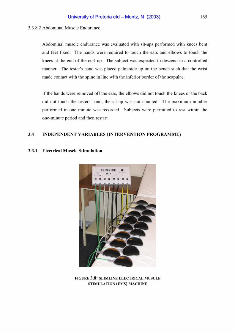
3.3.1 Electrical Muscle Stimulation

FIGURE 3.8: SLIMLINE ELECTRICAL MUSCLE STIMULATION (EMS) MACHINE


166

Electrical muscle stimulation (EMS) was performed using a Slimline EMS machine.

According to the suppliers, Slimline is a unique type of electro-medical apparatus,

which ensures that, a perfectly balanced exchange of electrons are constantly flowing

between each set of electro pads during treatment. A “Set of pads” consists of one (+)

pad and one (-) pad both of which are plugged into one of the eight channels of the

Slimline machine, thus providing a total of 16 pads. A greater sensation of contraction

is experienced in the region of the (+) pad or positive electrode. This is considered

normal and, necessary if treatment is to be effective (Slimline Promotional Literature,

2001).

Slimline slimming machines have three different electrokinetic modulations which

perform their functions at varying exercise levels and muscle depths, working in

gradual stages, from the deepest or basal muscles to the middle layers and finally to

the surface muscle layers. The entire treatment session is controlled by Slimline’s

computer, which varies all the modulations, depth of therapy and exercise levels

automatically. Pad placements are done according to pad placement charts, provided

by the manufacturer. The complete pad placement chart is included in Appendix D.

Each subject used the machine for eight weeks, twice per week for a duration of 45

minutes per session. The training frequency was selected according to the

manufacturer’s recommendation of at least two training sessions per week for

maximum results.


167

3.4.2 Thermogenic Stimulation

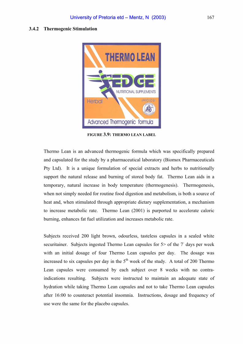
FIGURE 3.9: THERMO LEAN LABEL

Thermo Lean is an advanced thermogenic formula which was specifically prepared

and capsulated for the study by a pharmaceutical laboratory (Biomox Pharmaceuticals

Pty Ltd). It is a unique formulation of special extracts and herbs to nutritionally

support the natural release and burning of stored body fat. Thermo Lean aids in a

temporary, natural increase in body temperature (thermogenesis). Thermogenesis,

when not simply needed for routine food digestion and metabolism, is both a source of

heat and, when stimulated through appropriate dietary supplementation, a mechanism

to increase metabolic rate. Thermo Lean (2001) is purported to accelerate caloric

burning, enhances fat fuel utilization and increases metabolic rate.

Subjects received 200 light brown, odourless, tasteless capsules in a sealed white

securitainer. Subjects ingested Thermo Lean capsules for 5> of the 7- days per week

with an initial dosage of four Thermo Lean capsules per day. The dosage was

increased to six capsules per day in the 5th week of the study. A total of 200 Thermo

Lean capsules were consumed by each subject over 8 weeks with no contra-

indications resulting. Subjects were instructed to maintain an adequate state of

hydration while taking Thermo Lean capsules and not to take Thermo Lean capsules

after 16:00 to counteract potential insomnia. Instructions, dosage and frequency of

use were the same for the placebo capsules.


168

Composition per serving

Thermo Lean Placebo

Carcinia Cambogia Extract 2000 mg

Gaurana Extract 910 mg

(Paullinia Cupana 22%)

White Willow Bark 200 mg

Yohambine 3% Extract 160 mg

Citrus Aurantium 125 mg

(Citrus 6% Extract)

Acetyl L-Carnitine 100 mg

L-Tyrosine 80 mg

Ginger Root 50 mg

(Zingiber Officinale)

Calcium D Pantothenate 40 mg

Chromium Polynicotinate 200 mcg

Cellulose 3415 mg

Collour Agent 250 mg

Total 3665.2 mg

3665 mg

FIGURE 3.10: COMPOSITION OF THERMOGENIC AGENT AND PLACEBO

3.4.3 Standardized Diet Program

The standardized dietary intervention program, labelled as the Metabolism Diet,

emphasised the maintenance of a normal diet, including appropriate amounts of

carbohydrates, protein and fat, viz.:

• Carbohydrates 55 percent

• Protein 15 percent

• Fats 30 percent

The complete daily Metabolism Diet is included in Appendix E.

In general the subjects consumed normal everyday food, eating different amounts of

food (calories) in three phases.


169

• Low calorie phase

At 1000 calories per day, this phase was designed for maximum weight-loss, while

subjects consumed a nutritionally balanced diet. This menu was followed for two

weeks.

• Booster phase

After two weeks on the low calorie phase the subjects were required to switch to

the booster menu plan with 300 more calories. This phase was designed to boost

the metabolic rate. The added calories during the booster phase were made up by

carbohydrates.

Subjects alternated between the low calorie (two weeks) and the booster phase

(one-week). This was done in order to prevent potential plateaus in the subject's

diet (slowing the metabolic rate).

• Re-entry phase

When subjects got to within 2 to 3 kg from their target goal-weight, they switched

to the re-entry phase. Subjects thus gradually increased their caloric consumption

to reduce the risk of gaining weight. This pre-maintenance period served to get

the subject's metabolism ready for normal eating.

In all phases, subjects ate four meals per day viz.: breakfast, lunch, dinner and a

metabo-meal which was similar to a late-night supper. By taking more frequent

meals, the subjects were able to avoid the feeling of hunger and fatigue often

associated with a diet.

Basic rules of the Metabolism Diet

Subjects were required to:

a) eat everything exactly as it was prescribed;

b) not eat anything more than indicated;

c) never skip a meal;


170

d) drink plenty of fluids - water (minimum of 2 - 3 glasses per day), diet

beverages, and iced tea.

e) avoid fruit juices (calorie drinks) or liquids high in sodium (e.g. tomato juice);

f) not add table salt to food, so as to prevent potential water retention, but to

obtain their salt intake naturally from foods;

g) remove all visible fat from meat or skin from chicken, before eating;

h) avoid all alcoholic beverages;

i) only consume fresh fruit and fresh or frozen vegetables. Canned products

were not permitted to be eaten.

3.5 STATISTICAL ANALYSIS

An independent statistician was consulted and utilized for all statistical analyses.

Standard descriptive statistics for central tendency (mean) and spread (standard

deviation) were applied to all variables measured. Differences between pre- and post-

test scores within the three experimental groups were determined by the Wilcoxon

signed rank test. The Kruskal-Wallis test for three or more independent groups was

adopted as the appropriate statistical technique for the between group inferential

analysis of the data. This test is a non-parametric equivalent to a one-way analysis of

variance (ANOVA) (Howel, 1992).

In all analyses the 95% level of confidence (p ≤ 0,05) was applied as the minimum to

interpret significant differences among sets of data. Where the null hypothesis of the

Kruskal-Wallis test was rejected (p ≤ 0,05), multiple comparisons were used to detect

differences between two groups (TS vs. EST, EST vs. ESP etc.) using Scheffe and

LSD (least sign difference) methods (Smit, 2002). All computations were performed

using the Statistical Package for Social Science (SPSS), Microsoft Windows release

9.0 (1999).

Documents

CHAPTER 3 METHODS AND PROCEDURES