Embed Size (px)
Citation preview

Chapter 3
One-Dimensional Systems
In this chapter we describe geometrical methods of analysis of one-dimensional dynam-ical systems, i.e., systems having only one variable. An example of such a system isthe space-clamped membrane having Ohmic leak current IL
C V = −gL(V − EL) . (3.1)
Here the membrane voltage V is a time-dependent variable, and the capacitance C, leakconductance gL and leak reverse potential EL are constant parameters described in theprevious chapter. We use this and other one-dimensional neural models to introduceand illustrate the most important concepts of dynamical system theory: equilibrium,stability, attractor, phase portrait, and bifurcation.
3.1 Electrophysiological Examples
The Hodgkin-Huxley description of dynamics of membrane potential and voltage-gatedconductances can be reduced to a one-dimensional system when all transmembraneconductances have fast kinetics. For the sake of illustration, let us consider a space-clamped membrane having leak current and a fast voltage-gated current Ifast havingonly one gating variable p,
C V = −Leak IL︷ ︸︸ ︷
gL(V − EL)−Ifast︷ ︸︸ ︷
g p (V − E) (3.2)
p = (p∞(V )− p)/τ(V ) (3.3)
with dimensionless parameters C = 1, gL = 1, and g = 1. Suppose that the gatingkinetic (3.3) is much faster than the voltage kinetic (3.2), which means that the voltage-sensitive time constant τ(V ) is very small, i.e. τ(V ) ¿ 1, in the entire biophysicalvoltage range. Then, the gating process may be treated as being instantaneous, andthe asymptotic value p = p∞(V ) may be used in the voltage equation (3.2) to reduce
55

56 One-Dimensional Systems
0 1 2 3 4 5 6 7 8 9 100
0.1
0.2
0.3
0.4
0.5
0.6
0.7
0.8
0.9
1
0 1 2 3 4 5 6 7 8 9 10-80
-70
-60
-50
-40
-30
-20
-10
0
10
20
Time (ms) Time (ms)
Act
ivat
ion
Var
iabl
e
Mem
bran
e V
olta
ge (
mV
)
m(t) V(t)τ(V) < 0.5
τ(V) < 0.1
τ(V) < 0.01
Instantaneous
Figure 3.1: Solution of the full system (3.2, 3.3) converges to that of the reducedone-dimensional system (3.4) as τ(V ) → 0
the two-dimensional system (3.2, 3.3) to a one-dimensional equation
C V = −gL(V − EL)−instantaneous Ifast︷ ︸︸ ︷g p∞(V ) (V − E) . (3.4)
This reduction introduces a small error of the order τ(V ) ¿ 1, as one can see inFig. 3.1.
Since the hypothetical current Ifast can be either inward (E > EL) or outward(E < EL), and the gating process can be either activation (p is m, as in Hodgkin-Huxley model) or inactivation (p is h), there are four fundamentally different choicesfor Ifast(V ), which we summarize in Fig. 3.2 and elaborate below.
INa,p
Currentinward
activation
inactivation
outward
Gat
ing
IK
Ih IKir
Figure 3.2: Four fundamental examples of voltage-gated currents having one gating variable. In thisbook we treat “hyperpolarization-activated” cur-rents Ih and IKir as being inactivating currents,which are turned off (inactivated via h) by depo-larization and turned on (deinactivated) by hyper-polarization; see discussion in Sect. 2.2.4.
3.1.1 I-V relations and dynamics
The four choices in Fig. 3.2 result in four simple one-dimensional models of the form(3.4)
INa,p-model , IK-model , Ih-model , and IKir-model .
These models might seem to be too simple for biologists, who can easily understandtheir behavior just by looking at the I-V relations of the currents depicted in Fig. 3.3

One-Dimensional Systems 57
activ
atio
n, m
inac
tivat
ion,
hgatin
ginward outward
currents
V
I(V)INa,p
V
I(V)IK
V
I(V)
IKirV
I(V)
Ih
negativeconductance
negativeconductance
Figure 3.3: Typical current-voltage (I-V) relations of the fourcurrents considered in this chap-ter. Shaded boxes correspond tonon-monotonic I-V relations hav-ing a region of negative conduc-tance (I ′(V ) < 0) in the biophys-ically relevant voltage range.
without using any dynamical systems theory. The models might also appear too simplefor mathematicians, who can easily understand their dynamics just by looking at thegraphs of the right-hand side of (3.4) without using any electrophysiological intuition.In fact, the models provide an invaluable learning tool, since they establish a bridgebetween electrophysiology and dynamical systems.
In Fig. 3.3 we plot typical steady-state current-voltage (I-V) relations of the fourcurrents considered above. Notice that the I-V curve is non-monotonic for INa,p andIKir but monotonic for IK and Ih, at least in the biophysically relevant voltage range.This subtle difference is an indication of the fundamentally different roles these currentsplay in neuron dynamics: The I-V relation in the first group has a region of “negativeconductance”, i.e., I ′(V ) < 0, which creates positive feedback between the voltage andthe gating variable (Fig. 3.4), and it plays an amplifying role in neuron dynamics. Werefer to such currents as being amplifying currents. In contrast, the currents in thesecond group have negative feedback between voltage and gating variable, and theyoften result in damped oscillation of the membrane potential, as we show in the nextchapter. We refer to such currents as being resonant currents. Most neural modelsinvolve a combination of at least one amplifying and one resonant current, as we discussin Chap. 5. The way these currents are combined determines whether the neuron is anintegrator or a resonator.
3.1.2 Leak + instantaneous INa,p
To ease our introduction into dynamical systems, we will use the INa,p-model
C V = I − gL(V − EL)−instantaneous INa,p︷ ︸︸ ︷
gNa m∞(V ) (V − ENa) (3.5)
with
m∞(V ) = 1/(1 + exp {(V1/2 − V )/k})

58 One-Dimensional Systems
activ
atio
n, m
inac
tivat
ion,
h
gatin
ginward outward
currents
depolarization
inwardcurrent
increasein m+
+ +
+
depolarization
outwardcurrent
increasein m-
- +
+
hyperpolarization
inwardcurrent
increasein h
- +
+
-hyperpolarization
outwardcurrent
increasein h+
+ +
+
positive feedback,amplifying current
negative feedback,resonant current +-
Figure 3.4: Feedback loopsbetween voltage and gatingvariables in the four modelspresented above.
throughout the rest of this chapter. (Some biologists refer to transient Na+ currentswith very slow inactivation as being persistent, since the current does not change muchon the time scale of 1 sec.) We measure the parameters
C = 10 µF I = 0 pA gL = 19 mS EL = −67 mVgNa = 74 mS V1/2 = 1.5 mV k = 16 mV ENa = 60 mV
using whole-cell patch clamp recordings of a layer 5 pyramidal neuron in visual cortexof a rat at room temperature. We prove in Ex. 3.3.8 and illustrate in Fig. 3.15 thatthe model approximates action potential upstroke dynamics of this neuron.
The model’s I-V relation, I(V ), is depicted in Fig. 3.5a. Due to the negativeconductance region in the I-V curve, this one-dimensional model can exhibit a numberof interesting non-linear phenomena, such as bistability, i.e. co-existence of the restingand excited states. From mathematical point of view, bistability occurs because theright-hand side function of the differential equation (3.5), depicted in Fig. 3.5b, is notmonotonic. In Fig. 3.6 we depict typical voltage time courses of the model (3.5) withtwo values of injected dc-current I and 16 different initial conditions. The qualitativebehavior in Fig. 3.6a is apparently bistable: depending on the initial condition, thetrajectory of the membrane potential goes either up to the excited state or down tothe resting state. In contrast, the behavior in Fig. 3.6b is monostable, since the restingstate does not exist. The goal of the dynamical system theory reviewed in this chapteris to understand why and how the behavior depends on the initial conditions and theparameters of the system.
3.2 Dynamical Systems
In general, dynamical systems can be continuous or discrete, depending on whetherthey are described by differential or difference equations. Continuous one-dimensional

One-Dimensional Systems 59
-60 -40 -20 0 20 40 60
-2
-1
0
1
-60 -40 -20 0 20 40 60-50
0
50
100
membrane potential (mV) membrane potential, V (mV)
curr
ent (
nA)
V=F(V)
F(V)=-I(V)/C
I(V)
INa,p(V)
IL(V)
a b
deriv
ativ
e of
mem
bran
e po
tent
ial (
mV
/ms)
Figure 3.5: a. I-V relations of the leak current, IL, fast Na+ current, INa, and combinedcurrent I(V ) = IL(V ) + INa(V ) in the INa,p-model (3.5). Dots denote I0(V ) data fromlayer 5 pyramidal cell in rat visual cortex. b. The right-hand side of the INa,p-model(3.5).
dynamical systems are usually written in the form
V = F (V ) , V (0) = V0 ∈ R , (3.6)
for example,V = −80− V , V (0) = −20 ,
where V is a scalar time-dependent variable denoting the current state of the system,V = Vt = dV/dt is its derivative with respect to time t, F is a scalar function (itsoutput is one-dimensional) that determines the evolution of the system, e.g., the right-hand side of (3.5) divided by C; see Fig. 3.5b. V0 ∈ R is an initial condition, and R isthe real line, i.e., a line of real numbers (Rn would be the n-dimensional real space).
In the context of dynamical systems, the real line R is called phase line or state line(phase space or state space for Rn) to stress the fact that each point in R correspondsto a certain perhaps inadmissible state of the system, and each state of the systemcorresponds to a certain point in R. For example, the state of the Ohmic membrane(3.1) is just its membrane potential V ∈ R. The state of the Hodgkin-Huxley model(see Sect. 2.3) is the four-dimensional vector (V, m, n, h) ∈ R4. The state of the INa,p-model (3.5) is again its membrane potential V ∈ R, because the value m = m∞(V ) isunequivocally defined by V .
When all parameters are constant, then the dynamical system is called autonomous.When at least one of the parameters is time-dependent, the system is non-autonomous,denoted as V = F (V, t).
To solve (3.6) means to find a function V (t) whose initial value is V (0) = V0
and whose derivative is F (V (t)) at each moment t ≥ 0. For example, the functionV (t) = V0 + at is an explicit analytical solution to the dynamical system V = a. Theexponentially decaying function V (t) = EL + (V0 − EL)e−gLt/C depicted in Fig. 3.7,

60 One-Dimensional Systems
0 1 2 3 4 5-60
-40
-20
0
20
40
0 1 2 3 4 5-60
-40
-20
0
20
40
mem
bran
e po
tent
ial,
V (m
V)
mem
bran
e po
tent
ial,
V (m
V)
time (ms) time (ms)
bistability (I=0) monostability (I=60)
V(t) V(t)
a b
excited excited
resting
Figure 3.6: Typical voltage trajectories of the INa,p-model (3.5) having different valuesof I.
V(t)=EL+(V
0-E
L)e-g
L t/C
EL
V0
time, t
mem
bran
e po
tent
ial,
V
V(0)V(h)
V(2h)V(3h)
Figure 3.7: Explicit analytical solution (V (t) = EL+(V0−EL)e−gLt/C) of linear equation(3.1) and corresponding numerical approximation (dots) using Euler method (3.7).
solid curve, is an explicit analytical solution to the linear equation (3.1) (check bydifferentiating).
Finding explicit solutions is often impossible even for such simple systems as (3.5),so most quantitative analysis is carried out via numerical simulations. The simplestprocedure to solve (3.6) numerically, known as first-order Euler method, substitutes(3.6) by the discretized system
(V (t + h)− V (t))/h = F (V (t))
where t = 0, h, 2h, 3h, . . . , is the discrete time and h is a small time step. Knowing thecurrent state V (t), we can find the next state point via
V (t + h) = V (t) + hF (V (t)) . (3.7)
Iterating this difference equation starting with V (0) = V0, we can approximate the an-alytical solution of (3.6), see dots in Fig. 3.7. The approximation has a noticeable error

One-Dimensional Systems 61
0 5 0 5-60
-50
-40
-30
-20
-10
0
10
20
30
40
-100 -50 0-100
-50
0
50
100
-50 0 50
0
20
40
60
80
100
time (ms)
mem
bran
e po
tent
ial,
V (m
V)
time (ms)
membrane potential, V (mV)membrane potential, V (mV)
V(t)
V(t)
V>0 V<0V=0
stable equilibrium
IL IL+INa
a b
stable equilibrium
unstable equilibrium
stable equilibrium
stable equilibrium
-100
-90
-80
-70
-60
-50
-40
-30
-20
-10
0
mem
bran
e po
tent
ial,
V (m
V)
grap
h of
F(V
)=V
grap
h of
F(V
)=V
Ileak-model INa,p-model
Figure 3.8: Graphs of the right-hand side functions of equations (3.1) and (3.5) andcorresponding numerical solutions starting from various initial conditions.
of order h, so scientific software packages, such as MATLAB, use more sophisticatedhigh-precision numerical methods.
In many cases, however, we do not need exact solutions, but rather qualitativeunderstanding of the behavior of (3.6) and how it depends on parameters and theinitial state V0. For example, we might be interested in the number of equilibrium(rest) points the system could have, whether the equilibria are stable, their attractiondomains, etc.
3.2.1 Geometrical analysis
The first step in qualitative geometrical analysis of any one-dimensional dynamicalsystem is to plot the graph of the function F , as we do in Fig. 3.8,top. Since F (V ) = V ,at every point V where F (V ) is negative, the derivative V is negative, and hence the

62 One-Dimensional Systems
state variable V decreases. In contrast, at every point where F (V ) is positive, V ispositive, and the state variable V increases; the greater the value of F (V ), the fasterV increases. Thus, the direction of movement of the state variable V , and hence theevolution of the dynamical system, is determined by the sign of the function F (V ).
The right-hand side of the Ileak-model (3.1) or the INa,p-model (3.5) in Fig. 3.8 is thesteady-state current-voltage (I-V) relation, IL(V ) or IL(V )+INa,p(V ) respectively, takenwith the minus sign, see Fig. 3.5. Positive values of the right-hand side F (V ) meannegative I-V corresponding to the net inward current that depolarizes the membrane.Conversely, negative values mean positive I-V corresponding to the net outward currentthat hyperpolarizes the membrane.
3.2.2 Equilibria
The next step in qualitative analysis of any dynamical system is to find its equilibriaor rest points, i.e., the values of the state variable where
F (V ) = 0 (V is an equilibrium).
At each such point V = 0, the state variable V does not change. In the context ofmembrane potential dynamics, equilibria correspond to the points where the steady-state I-V curve passes zero. At each such point there is a balance of the inward andoutward currents so that the net transmembrane current is zero, and the membranevoltage does not change. (Incidentally, the part l ibra in the Latin word aequil ibriummeans balance).
The IK- and Ih-models mentioned in Sect. 3.1 can have only one equilibrium be-cause their I-V relations I(V ) are monotonic increasing functions. The correspondingfunctions F (V ) are monotonic decreasing and can have only one zero.
In contrast, the INa,p- and IKir-models can have many equilibria because their I-Vcurves are not monotonic, and hence there is a possibility for multiple intersectionswith the V -axis. For example, there are three equilibria in Fig. 3.8b correspondingto the rest state (around -53 mV), threshold state (around -40 mV) and the excitedstate (around 30 mV). Each equilibrium corresponds to the balance of the outwardleak current and partially (rest), moderately (threshold) or fully (excited) activatedpersistent Na+ inward current. Throughout this book we denote equilibria as smallopen or filled circles depending on their stability, as in Fig. 3.8.
3.2.3 Stability
If the initial value of the state variable is exactly at equilibrium, then V = 0 and thevariable will stay there forever. If the initial value is near the equilibrium, the statevariable may approach the equilibrium or diverge from it. Both cases are depicted inFig. 3.8. We say that an equilibrium is asymptotically stable if all solutions startingsufficiently near the equilibrium will approach it as t →∞.

One-Dimensional Systems 63
V
F (V)<0
negative slope
F(V)
V
F (V)>0
positive slope
F(V)
stableequilibrium
unstableequilibrium
Figure 3.9: The sign of the slope,λ = F ′(V ), determines the stabilityof the equilibrium.
Stability of an equilibrium is determined by the signs of the function F around it.The equilibrium is stable when F (V ) changes the sign from “+” to “−” as V increases,as in Fig. 3.8a. Obviously, all solutions starting near such an equilibrium converge toit. Such an equilibrium “attracts” all nearby solutions, and it is called an attractor. Astable equilibrium point is the only type of attractor that can exist in one-dimensionalcontinuous dynamical systems defined on a state line R. Multidimensional systems canhave other attractors, e.g., limit cycles.
The differences between stable, asymptotically stable, and exponentially stableequilibria are discussed in Ex. 19 in the end of the chapter. The reader is also en-couraged to solve Ex. 4 (piece-wise continuous F (V )).
3.2.4 Eigenvalues
A sufficient condition for an equilibrium to be stable is that the derivative of thefunction F with respect to V at the equilibrium is negative, provided that the functionis differentiable. We denote such a derivative here by the Greek letter
λ = F ′(V ) , (V is an equilibrium; that is, F (V ) = 0)
and note that it is just the slope of graph of F at the point V ; see Fig. 3.9. Obviously,when the slope, λ, is negative, the function changes the sign from “+” to “−”, andthe equilibrium is stable. Positive slope λ implies instability. The parameter λ definedabove is the simplest example of an eigenvalue of an equilibrium. We introduce eigen-values formally in the next chapter and show that eigenvalues play an important rolein defining the types of equilibria of multi-dimensional systems.
3.2.5 Unstable equilibria
If a one-dimensional system has two stable equilibrium points, then they must beseparated by at least one unstable equilibrium point, as we illustrate in Fig. 3.10.(This may not be true in multidimensional systems.) Indeed, a continuous functionF has to change the sign from “−” to “+” somewhere in between those equilibria;that is, it has to cross the V axis in some point, as in Fig. 3.8b. This point would be

64 One-Dimensional Systems
V
F(V)>0
F(V)<0
+ +- -
??
?
?
- +
Figure 3.10: Two stable equilibrium points must be separated by at least one unstableequilibrium point because F (V ) has to change the sign from “−” to “+”.
an unstable equilibrium, since all nearby solutions diverge from it. In the context ofneuronal models, unstable equilibria correspond to the region of the steady-state I-Vcurve with negative conductance. (Please, check that this is in accordance with thefact that F (V ) = −I(V )/C; see Fig. 3.5.) An unstable equilibrium is sometimes calleda repeller. Attractors and repellers have a simple mechanistic interpretation depictedin Fig. 3.11.
If the initial condition V0 is set to an unstable equilibrium point, then the solutionwill stay at this unstable equilibrium; i.e., V (t) = V0 for all t, at least in theory. Inpractice, the location of an equilibrium point is known only approximately. In addition,small noisy perturbations that are always present in biological systems can make V (t)deviate slightly from the equilibrium point. Because of instability, such deviations willgrow, and the state variable V (t) will eventually diverge form the repelling equilibriumthe same way as the ball set at the top of the hill in Fig. 3.11 will eventually rolldownhill. If the level of noise is low, it could take a long time to diverge from therepeller.
3.2.6 Attraction domain
Even though unstable equilibria are hard to see experimentally, they still play an im-portant role in dynamics, since they separate attraction domains. Indeed, the ball inFig. 3.11 could go left or right depending on what side of the hilltop it is on initially.Similarly, the state variable of a one-dimensional system decreases or increases depend-ing on what side of the unstable equilibrium the initial condition is, as one can clearlysee in Fig. 3.8b.
In general, a basin of attraction or attraction domain of an attractor is the set of allinitial conditions that lead to the attractor. For example, the attraction domain of theequilibrium in Fig. 3.8a is the entire voltage range. Such an attractor is called global.In Fig. 3.12 we plot attraction domains of two stable equilibria. The middle unstableequilibrium is always the boundary of the attraction domains.

One-Dimensional Systems 65
���������������������������������������������������������������������������������
����������������������������������������������������������������������������������������������������������������������������������������������������������������������������������������������������������������������������������������������������������������������������������������������������������������������������������������������������������������������������������������������������������������������������������������������������������������������������������������������������������������������������������������������������������������������������������������������������������������������������������������������������������������������������������������������������������������������������������������������������������������������������������������������������������������������������������������������������������������������������������������������������������������������������������������������������������������������������������������������������������������������������������������������������������������������������������������������������������������������������������������������������������������������������������������������������������������������������������������������������������������������������������������������������������������������������������������������������������������������������������������������������������������������������������������������������������������������������������������������������������������������������������������������������������������������������������������������������������������������������������������������������������������������������������������������������������������������������������������������������������������������������������������������������������������������������������������������������������������������������������������������������������������������������������������������������������������������������������������������������������������������������������������������������������������������������������������������������������������������������������������������������������������������������������������������������������������������������������������������������������������������������������������������������������������������������������������������������������������������������������������������������������������������������������������������������������������������������������������������������������������������������������������������������������������������������������������������������������������������������������������������������������������������������������������������������������������������������������������������������������������������������������������������������������������������������������������������������������������������������������������������������������������������������������������������������������������������������������������������������������������������������������������������������������������������������������������������������������������������������������������������������������������������������������������������������������������������������������������������������������������������������������������������������������������������������������������������������
F(V)
V
- F(v)dv
Figure 3.11: Mechanistic interpretation of stable and unstable equilibria. A massless(inertia free) ball moves toward energy minima with the speed proportional to the slope.
A one-dimensional system V = F (V ) has the energy landscape E(V ) = − ∫ V
−∞ F (v) dv;see Ex. 18. Zeros of F (V ) with negative (positive) slope correspond to minima (max-ima) of E(V ).
3.2.7 Threshold and action potential
Unstable equilibria play the role of thresholds in one-dimensional bistable systems, i.e.,in systems having two attractors. We illustrate this in Fig. 3.13, which is believed todescribe the essence of the mechanism of bistability in many neurons. Suppose the statevariable is initially at the stable equilibrium point marked as “state A” in the figure,and suppose that perturbations can kick it around the equilibrium. Small perturbationsmay not kick it over the unstable equilibrium so that the state variable continues tobe in the attraction domain of the “state A”. We refer to such perturbations as beingsubthreshold. In contrast, we refer to perturbations as being superthreshold (also knownas suprathreshold) if they are large enough to push the state variable over the unstableequilibrium so that it becomes attracted to the “state B”. We see that the unstableequilibrium acts as a threshold that separates two states.
The transition between two stable states separated by a threshold is relevant to themechanism of excitability and generation of action potentials by many neurons, whichwe illustrate in Fig. 3.14. In the INa,p-model (3.5) with the I-V relation in Fig. 3.5the existence of the rest state is largely due to the leak current IL, while the existenceof the excited state is largely due to the persistent inward Na+ current INa,p. Small

66 One-Dimensional Systems
F(V)
V
Attraction Domain
Attraction Domain
Unstable Equilibrium
Figure 3.12: Two attraction domains in a one-dimensional system are separated by theunstable equilibrium.
(subthreshold) perturbations leave the state variable in the attraction domain of therest state, while large (superthreshold) perturbations initiate the regenerative process— the upstroke of an action potential, and the voltage variable becomes attracted to theexcited state. Generation of the action potential must be completed via repolarizationthat moves V back to the rest state. Typically, repolarization occurs because of arelatively slow inactivation of Na+ current and/or slow activation of an outward K+
current, which are not taken into account in the one-dimensional system (3.5). Toaccount for such processes, we consider two-dimensional systems in the next chapter.
Recall that the parameters of the INa,p-model (3.5) were obtained from a corticalpyramidal neuron. In Fig. 3.15, left, we stimulate (in vitro) the cortical neuron by short(0.1 ms) strong pulses of current to reset its membrane potential to various initial valuesand interpret the results using the INa,p-model. Since activation of Na+ current is notinstantaneous in real neurons, we allow variable m to converge to m∞(V ), and ignorethe 0.3-ms transient activity that follows each pulse. We also ignore the initial segmentof the downstroke of the action potential, and plot the magnification of the voltagetraces in Fig. 3.15, right. Comparing this figure with Fig. 3.8b, we see that the INa,p-model is a reasonable one-dimensional approximation of the action potential upstrokedynamics; It predicts the value of the resting (-53 mV), instantaneous threshold (-40mV), and the excited (+30 mV) states of the cortical neuron.
3.2.8 Bistability and hysteresis
Systems having two (many) co-existing attractors are called bistable (multi-stable).Many neurons and neuronal models, such as the Hodgkin-Huxley model, exhibit bista-bility between resting (equilibrium) and spiking (limit cycle) attractors. Some neuronscan exhibit bistability of two stable resting states in the subthreshold voltage range,e.g., -59 mV and -75 mV in the thalamocortical neurons (Hughes et al. 1999) depicted

One-Dimensional Systems 67
������������������������������������������������������������������������
�����������������������������������������������������������������������������������������������������������������������������������������������������������������������������������������������������������������������������������������������������������������������������������������������������������������������������������������������������������������������������������������������������������������������������������������������������������������������������������������������������������������������������������������������������������������������������������������������������������������������������������������������������������������������������������������������������������������������������������������������������������������������������������������������������������������������������������������������������������������������������������������������������������������������������������������������������������������������������������������������������������������������������������������������������������������������������������������������������������������������������������������������������������������������������������������������������������������������������������������������������������������������������������������������������������������������������������������������������������������������������������������������������������������������������������������������������������������������������������������������������������������������������������������������������������������������������������������������������������������������������������������������������������������������������������������������������������������������������������������������������������������������������������������������������������������������������������������������������������������������������������������������������������������������������������������������������������������������������������������������������������������������������������������������������������������������������������������������������������������������������������������������������������������������������������������������������������������������������������������������������������������������������������������������������������������������������������������������������������������������������������������������������������������������������������������������������������������������������������������������������������������������������������������������������������������������������������������������������������������������������������������������������������������������������������������������������������������������������������������������������������������������������������������������������������������������������������������������������������������������������������������������������������������������������������������������������������������������������������������������������������������������������������������������������������������������������������������������������������������������������������������������������������������������������������������������������������������������������������������������������������������������������������������������������������������������������������������������������������������������������������������������������������������������������������������������������������������������
F(V)
V
���������������������������������������������������������������������������������
����������������������������������������������������������������������������������������������������������������������������������������������������������������������������������������������������������������������������������������������������������������������������������������������������������������������������������������������������������������������������������������������������������������������������������������������������������������������������������������������������������������������������������������������������������������������������������������������������������������������������������������������������������������������������������������������������������������������������������������������������������������������������������������������������������������������������������������������������������������������������������������������������������������������������������������������������������������������������������������������������������������������������������������������������������������������������������������������������������������������������������������������������������������������������������������������������������������������������������������������������������������������������������������������������������������������������������������������������������������������������������������������������������������������������������������������������������������������������������������������������������������������������������������������������������������������������������������������������������������������������������������������������������������������������������������������������������������������������������������������������������������������������������������������������������������������������������������������������������������������������������������������������������������������������������������������������������������������������������������������������������������������������������������������������������������������������������������������������������������������������������������������������������������������������������������������������������������������������������������������������������������������������������������������������������������������������������������������������������������������������������������������������������������������������������������������������������������������������������������������������������������������������������������������������������������������������������������������������������������������������������������������������������������������������������������������������������������������������������������������������������������������������������������������������������������������������������������������������������������������������������������������������������������������������������������������������������������������������������������������������������������������������������������������������������������������������������������������������������������������������������������������������������������������������������������������������������������������������������������������������������������������������������������������������������������������������������������������������
state A state B
state A
state A
state B
state B
subthresholdperturbation
superthresholdperturbation
Attraction domainof state A
Attraction domainof state B
threshold
threshold
threshold
Figure 3.13: Unstable equilibrium plays the role of a threshold that separates twoattraction domains.

68 One-Dimensional Systems
depolarization
hyperpolarization
��������������������������������������������������������
�����������������������������������������������������������������������������������������������������������������������������������������������������������������������������������������������������������������������������������������������������������������������������������������������������������������������������������������������������������������������������������������������������������������������������������������������������������������������������������������������������������������������������������������������������������������������������������������������������������������������������������������������������������������������������������������������������������������������������������������������������������������������������������������������������������������������������������������������������������������������������������������������������������������������������������������������������������������������������������������������������������������������������������������������������������������������������������������������������������������������������������������������������������������������������������������������������������������������������������������������������������������������������������������������������������������������������������������������������������������������������������������������������������������������������������������������������������������������������������������������������������������������������������������������������������������������������������������������������������������������������������������������������������������������������������������������������������������������������������������������������������������������������������������������������������������������������������������������������������������������������������������������������������������������������������������������������������������������������������������������������������������������������������������������������������������������������������������������������������������������������������������������������������������������������������������������������������������������������������������������������������������������������������������������������������������������������������������������������������������������������������������������������������������������������������������������������������������������������������������������������������������������������������������������������������������������������������������������������������������������������������������������������������������������������������������������������������������������������������������������������������������������������������������������������������������������������������������������������������������������������������������������������������������������������������������������������������������������������������������������������������������������������������������������������������������������������������������������������������������������������������������������������������������������������������������������������������������������������������������������������������������������������������������������������������������������������������������������������������������������������������������������������������������������������������������������������������������������
rest state
excited
superthresholdperturbation
upstroke
repolarization
regenerative
IK
INa
threshold
(another variable)
Figure 3.14: Mechanistic illustration of the mechanism of generation of an action po-tential.
-40 mV
0 0.2 0.4 0.6 0.8 1 1.2-60
-50
-40
-30
-20
-10
0
10
20
30
40
1 ms
time (ms)
mem
bran
e po
tent
ial (
mV
)
20 mVstable equilibrium
unstable equilibrium
stable equilibrium
mem
bran
e po
tent
ial (
mV
)
pulses of current
strong depolarization
action potentials
+30 mV
Figure 3.15: Upstroke dynamics of layer 5 pyramidal neuron in vitro (compare withthe INa,p-model (3.5) in Fig. 3.8b).
One-Dimensional Systems 69
-59 mV
-75 mV
2 s100 pA
15 mV
mem
bran
e po
tent
ial
Figure 3.16: Membrane potential bistability in a cat TC neuron in the presence ofZD7288 (pharmacological blocker of Ih; modified from Fig. 6B of Hughes et al. 1999).
V
I+F(V)
(a)
(b)
(c)
(d)
(a)
(b)
(c)
(b)
V
I
Figure 3.17: Bistability and hysteresis loop as I changes.
in Fig. 3.16, or -50 mV and -60 mV in mitral cells of olfactory bulb (Heyward et al.2001), or -45 mV and -60 mV in Purkinje neurons. Brief inputs can switch such neu-rons from one state to the other, as in Fig. 3.16. Though the ionic mechanisms ofbistability are different in the three neurons, the mathematical mechanism is the same.
Consider a one-dimensional system V = I + F (V ) with function F (V ) having acubic N-shape. Injection of a dc-current I shifts the function I + F (V ) up or down.When I is negative, the system has only one equilibrium depicted in Fig. 3.17a. As weremove the injected current I, the system is bistable as in Fig. 3.17b, but its state isstill at the left equilibrium. As we inject positive current, the left stable equilibriumdisappears via another saddle-node bifurcation, and the state of the system jumps tothe right equilibrium, as in Fig. 3.17c. But as we slowly remove the injected currentthat caused the jump and go back to Fig. 3.17b, the jump to the left equilibriumdoes not occur until a much lower value corresponding to Fig. 3.17a. The failure ofthe system to return to the original value when the injected current is removed iscalled hysteresis. If I were a slow V -depended variable, then the system could exhibitrelaxation oscillations depicted in Fig. 3.17d and described in the next chapter.

70 One-Dimensional Systems
V+ - + - + - + -+- +- +-
V
Phase Portrait
Function F(V)
Attraction domains
Figure 3.18: Phase portrait of a one-dimensional system V = F (V ).
V
V
F (V)1
F (V)2
Figure 3.19: Two “seemingly different”dynamical systems V = F1(V ) andV = F2(V ) are topologically equiv-alent, hence they have qualitativelysimilar dynamics.
3.3 Phase Portraits
An important component in qualitative analysis of any dynamical system is reconstruc-tion of its phase portrait. For this one depicts all stable and unstable equilibria (asblack and white circles respectively), representative trajectories, and corresponding at-traction domains in the systems state/phase space, as we illustrate in Fig. 3.18. Phaseportrait is a geometrical representation of system dynamics. It depicts all possibleevolutions of the state variable and how they depend on the initial state. Looking atthe phase portrait, one immediately gets all important information about the systemqualitative behavior without even knowing the equation for F .

One-Dimensional Systems 71
V
V
? F (V)2
F (V)1
Figure 3.20: Two “seemingly alike”dynamical systems V = F1(V ) andV = F2(V ) are not topologicallyequivalent, hence they do not havequalitatively similar dynamics. (Thefirst system has three equilibria, andthe second system has only one.)
3.3.1 Topological equivalence
Phase portraits can be used to determine qualitative similarity of dynamical systems.In particular, two one-dimensional systems are said to be topologically equivalent whenphase portrait of one of them treated as a piece of rubber can be stretched or shrunkto fit the other one, as in Fig. 3.19. Topological equivalence is a mathematical conceptthat clarifies the imprecise notion of “qualitative similarity”, and its rigorous definitionis provided, e.g., by Guckenheimer and Holmes (1983).
The stretching and shrinking of the “rubber” phase space are topological trans-formations that do not change the number of equilibria or their stability. Thus, twosystems having different number of equilibria cannot be topologically equivalent, hencethey have qualitatively different dynamics, as we illustrate in Fig. 3.20. Indeed, the topsystem is bistable because it has two stable equilibria separated by an unstable one.The evolution of the state variable depends on which attraction domain the initial con-dition is in initially. Such a system has “memory” of the initial condition. Moreover,sufficiently strong perturbations can switch it from one equilibrium state to another.In contrast, the bottom system in Fig. 3.20 has only one equilibrium, which is a globalattractor, and the state variable converges to it regardless of the initial condition. Sucha system has quite primitive dynamics, and it is topologically equivalent to the linearsystem (3.1).
3.3.2 Local equivalence and Hartman-Grobman theorem
In computational neuroscience, we usually face quite complicated systems describingneuronal dynamics. A useful strategy is to substitute such systems by simpler oneshaving topologically equivalent phase portraits. For example, both systems in Fig. 3.19are topologically equivalent to V = V − V 3 (please, check this), which is easier to dealwith analytically.
Quite often we cannot find a simpler system that is topologically equivalent to ourneuronal model on the entire state line R. In this case, we make a sacrifice: we restrict

72 One-Dimensional Systems
V
F(V)
Veq
λ(V-Veq)
Figure 3.21: Hartman-Grobman theo-rem: Non-linear system V = F (V ) istopologically equivalent to the linear oneV = λ(V − Veq) in the local (shaded)neighborhood of the hyperbolic equilib-rium Veq.
our analysis to a small neighborhood of the line R, e.g., the one containing the restingstate or the threshold, and study behavior locally in this neighborhood.
An important tool in local analysis of dynamical systems is the Hartman-Grobmantheorem, which says that a non-linear one-dimensional system
V = F (V )
sufficiently near an equilibrium V = Veq is locally topologically equivalent to the linearone
V = λ(V − Veq) (3.8)
provided that the eigenvalueλ = F ′(Veq)
at the equilibrium is non-zero, i.e., the slope of F (V ) is non-zero. Such an equilibriumis called hyperbolic. Thus, nonlinear systems near hyperbolic equilibria behave as ifthere were linear, as in Fig. 3.21.
It is easy to find the exact solution of the linearized system (3.8) with an initialcondition V (0) = V0. It is V (t) = Veq + eλt(V0 − Veq) (check by differentiating).If the eigenvalue λ < 0, then eλt → 0 and V (t) → Veq as t → ∞, so that theequilibrium is stable. Conversely, if λ > 0, then eλt → ∞ meaning that the initialdisplacement, V0 − Veq, grows with the time, and the equilibrium is unstable. Thus,the linearization predicts qualitative dynamics at the equilibrium and quantitative rateof convergence/divergence to/from the equilibrium.
If the eigenvalue λ = 0, then the equilibrium is non-hyperbolic, and analysis ofthe linearized system V = 0 cannot describe the behavior of the nonlinear system.Typically, non-hyperbolic equilibria arise when the system undergoes a bifurcation,i.e., a qualitative change of behavior, which we consider next. To study stability, weneed to consider higher-order terms of the Taylor series of F (V ) at Veq.
3.3.3 Bifurcations
The final and the most advanced step in qualitative analysis of any dynamical systemis the bifurcation analysis. In general, a system is said to undergo a bifurcation whenits phase portrait changes qualitatively. For example, the energy landscape in Fig. 3.22changes so that the system is no longer bistable. Precise mathematical definition of abifurcation will be given later.

One-Dimensional Systems 73
������������������������������������������������������������������������
��������������������������������������������������������������������������������������������������������������������������������������������������������������������������������������������������������������������������������������������������������������������������������������������������������������������������������������������������������������������������������������������������������������������������������������������������������������������������������������������������������������������������������������������������������������������������������������������������������������������������������������������������������������������������������������������������������������������������������������������������������������������������������������������������������������������������������������������������������������������������������������������������������������������������������������������������������������������������������������������������������������������������������������������������������������������������������������������������������������������������������������������������������������������������������������������������������������������������������������������������������������������������������������������������������������������������������������������������������������������������������������������������������������������������������������������������������������������������������������������������������������������������������������������������������������������������������������������������������������������������������������������������������������������������������������������������������������������������������������������������������������������������������������������������������������������������������������������������������������������������������������������������������������������������������������������������������������������������������������������������������������������������������������������������������������������������������������������������������������������������������������������������������������������������������������������������������������������������������������������������������������������������������������������������������������������������������������������������������������������������������������������
���������������������������������������������������������������������������������
�������������������������������������������������������������������������������������������������������������������������������������������������������������������������������������������������������������������������������������������������������������������������������������������������������������������������������������������������������������������������������������������������������������������������������������������������������������������������������������������������������������������������������������������������������������������������������������������������������������������������������������������������������������������������������������������������������������������������������������������������������������������������������������������������������������������������������������������������������������������������������������������������������������������������������������������������������������������������������������������������������������������������������������������������������������������������������������������������������������������������������������������������������������������������������������������������������������������������������������������������������������������������������������������������������������������������������������������������������������������������������������������������������������������������������������������������������������������������������������������������������������������������������������������������������������������������������������������������������������������������������������������������������������������������������������������������������������������������������������������������������������������������������������������������������������������������������������������������������������������������������������������������������������������������������������������������������������������������������������������������������������������������������������������������������������������������������������������������������������������������������������������������������������������������������������������������������������������������������������������������������������������������
���������������������������������������������������������������������������������������������������������������������
�������������������������������������������������������������������������������������������������������������������������������������������������������������������������������������������������������������������������������������������������������������������������������������������������������������������������������������������������������������������������������������������������������������������������������������������������������������������������������������������������������������������������������������������������������������������������������������������������������������������������������������������������������������������������������������������������������������������������������������������������������������������������������������������������������������������������������������������������������������������������������������������������������������������������������������������������������������������������������������������������������������������������������������������������������������������������������������������������������������������������������������������������������������������������������������������������������������������������������������������������������������������������������������������������������������������������������������������������������������������������������������������������������������������������������������������������������������������������������������������������������������������������������������������������������������������������������������������������������������������������������������������������������������������������������������������������������������������������������������������������������������������������������������������������������������������������������������������������������������������������������������������������������������������������������������������������������������������������������������������������������������������������������������������������������������������������������������������������������������������������������������������������������������������������������������������������������������������������������������������������������������������������
Bifurcation
Bistability
Monostability
Figure 3.22: Mechanistic illustration of a bifurcation as a change of the landscape.
Qualitative change of the phase portrait may or may not necessarily reveal itselfin a qualitative change of behavior, depending on the initial conditions. For example,there is a bifurcation in Fig. 3.23, left, but no change of behavior because the ballremains in the attraction domain of the right equilibrium. To see the change, we needto drop the ball at different initial conditions and observe the disappearance of the leftequilibrium. In the same vain, there is no bifurcation Fig. 3.23, middle and right, (thephase portraits in each column are topologically equivalent) but the apparent change ofbehavior is caused by the expansion of the attraction domain of the left equilibrium orby the external input. Dropping the ball at different locations would result in the samequalitative picture – two stable equilibria whose attraction domains are separated bythe unstable equilibrium. When mathematicians talk about bifurcations, they assumethat all initial conditions could be sampled, in which case bifurcations do result in aqualitative change of behavior of the system as a whole.
To illustrate the importance of sampling all initial conditions, let us consider the invitro recordings of a pyramidal neuron in Fig. 3.24. We inject 0.1-ms strong pulses ofcurrent of various amplitude to set the membrane potential to different initial values.Right after each pulse, we inject a 4 ms step of dc-current of amplitude I = 0, I = 16or I = 60 pA. The case I = 0 pA is the same as in Fig. 3.15, so some initial conditions

74 One-Dimensional Systems
bifurcation but no change of behavior
change of behavior but no bifurcation
pulsed input
Figure 3.23: Bifurcations are not equivalent to qualitative change of behavior if thesystem is started with the same initial condition or subject to external input.
-40 mV
1 ms
10 mV
I=0 I=16 I=60dc-current dc-current dc-current
mem
bran
e po
tent
ial,
mV
pulses pulses pulses
bistable monostablebistable
Figure 3.24: Qualitative change of the up-stroke dynamics of layer 5 pyramidal neuronfrom rat visual cortex (the same neuron as in Fig. 3.15).

One-Dimensional Systems 75
result in upstroke of the action potential, while others do not. When I = 60 pA, allinitial conditions result in the generation of an action potential. Apparently, a changeof qualitative behavior occurs for some I between 0 and 60.
To understand the qualitative dynamics in Fig. 3.24, we consider the one-dimensionalINa,p-model (3.5) having different values of the parameter I and depict its trajectoriesin Fig. 3.25. One can clearly see that the qualitative behavior of the model dependson whether I is greater or less than 16. When I = 0 (top of Fig. 3.25), the system isbistable. The rest and the excited states coexist. When I is large (bottom of Fig. 3.25)the rest state no longer exists because leak outward current cannot cope with largeinjected dc-current I and the inward Na+ current.
What happens when we change I past 16? The answer lies in the details of thegeometry of the right-hand side function F (V ) of (3.5) and how it depends on theparameter I. Increasing I elevates the graph of F (V ). The higher the graph of F (V )is, the closer its intersections with the V -axis are, as we illustrate in Fig. 3.26 depictingonly the low-voltage range of the system. When I approaches 16, the distance betweenthe stable and unstable equilibria vanishes; the equilibria coalesce and annihilate eachother. The value I = 16 at which the equilibria coalesce is called the bifurcation value.This value separates two qualitatively different regimes: When I is near but less than16, the system has three equilibria and bistable dynamics. The quantitative features,such as the exact locations of the equilibria depend on the particular values of I, butqualitative behavior remains unchanged no matter how close I to the bifurcation valueis. In contrast, when I is near but greater than 16 the system has only one equilibriumand monostable dynamics.
In general, a dynamical system may depend on a vector of parameters, say p. Apoint in the parameter space, say p = a, is said to be a regular or non-bifurcation point,if the system’s phase portrait at p = a is topologically equivalent to the phase portraitat p = c for any c sufficiently near a. For example, the value I = 13 in Fig. 3.26 isregular, since the system has topologically equivalent phase portraits for all I near 13.Similarly, the value I = 18 is also regular. Any point in the parameter space that is notregular is called a bifurcation point. Namely, a point p = b is a bifurcation point, if thesystem’s phase portrait at p = b is not topologically equivalent to the phase portraitat some point p = c no matter how close c to b is. The value I = 16 in Fig. 3.26 is abifurcation point. It corresponds to the saddle-node (also known as fold or tangent)bifurcation for reasons described later. It is one of the simplest bifurcations consideredin this book.
3.3.4 Saddle-node (fold) bifurcation
In general, a one-dimensional system
V = F (V, I)
having an equilibrium point V = Vsn for some value of the parameter I = Isn (i.e.,F (Vsn, Isn) = 0) is said to be at a saddle-node bifurcation (sometimes called a fold

76 One-Dimensional Systems
0
20
40
60
80
100
0
20
40
60
80
100
-50 0 50
0
20
40
60
80
100
-60
-40
-20
0
20
40
-60
-40
-20
0
20
40
0 1 2 3 4 5-60
-40
-20
0
20
40
membrane potential, V (mV)
mem
bran
e po
tent
ial,
V (m
V)
mem
bran
e po
tent
ial,
V (m
V)
mem
bran
e po
tent
ial,
V (m
V)
threshold
excited state
excited state
excited state
rest
F(V)
F(V)
F(V)
I=0
I=16
I=60
bistability
bifurcation
monostability
tangent point
rest threshold
time (ms)
V(t)
V(t)
V(t)
Figure 3.25: Bifurcation in the INa,p-model (3.5): The rest state and the thresholdstate coalesce and disappear when the parameter I increases.

One-Dimensional Systems 77
F(V)
stable equilibria
point
unstable equilibria
V
I=16
I=15
I=14
I=13I=12
I=11
I=17
I=18
tangent
no equilibria
bifurcation
two equilibria
Figure 3.26: Saddle-node bifurcation: While the graph of the function F (V ) is liftedup, the stable and unstable equilibria approach each other, coalesce at the tangentpoint, and then disappear.
non-hyperbolic hyperbolic
non-degenerate degenerate degenerate
transversal not transversal
hyperbolic
F
not transversal
V
saddle-node not saddle-node
Figure 3.27: Geometrical illustration of the three conditions defining saddle-node bi-furcations. Arrows denote the direction of displacement of the function F (V, I) as thebifurcation parameter I changes.

78 One-Dimensional Systems
bifurcation) if the following mathematical conditions, illustrated in Fig. 3.27, are sat-isfied:
• (Non-hyperbolicity) The eigenvalue λ at Vsn is zero; that is,
λ = FV (V, Isn) = 0 (at V = Vsn),
where FV means the derivative of F with respect to V , that is, FV = ∂F/∂V .Equilibria with zero or pure imaginary eigenvalues are called non-hyperbolic.Geometrically, this condition implies that the graph of F has horizontal slope atthe equilibrium.
• (Non-degeneracy) The second order derivative with respect to V at Vsn is non-zero; that is,
FV V (V, Isn) 6= 0 (at V = Vsn).
Geometrically, this means that the graph of F looks like the square parabola V 2
in Fig. 3.27.
• (Transversality) The function F (V, I) is non-degenerate with respect to the bi-furcation parameter I; that is,
FI(Vsn, I) 6= 0 (at I = Isn),
where FI means the derivative of F with respect to I. Geometrically, this meansthat while I changes past Isn, the graph of F approaches, touches, and thenintersects the V axis.
Saddle-node bifurcation results in appearance or disappearance of a pair of equilibria,as in Fig. 3.26. None of the six examples on the right-hand side of Fig. 3.27 can undergoa saddle-node bifurcation because at least one of the conditions above is violated.
The number of conditions involving strict equality (“=”) is called the co-dimensionof a bifurcation. The saddle-node bifurcation has co-dimension-1 because there is onlyone condition involving “=”, and the other two conditions involve inequalities (“ 6=”).Co-dimension-1 bifurcations can be reliably observed in systems with one parameter.
It is an easy exercise to check that the one-dimensional system
V = I + V 2 (3.9)
is at saddle-node bifurcation when V = 0 and I = 0 (please, check all three conditions).This system is called the topological normal form for saddle-node bifurcation. Phaseportraits of this system are topologically equivalent to those depicted in Fig. 3.26 exceptthat the bifurcation occurs at I = 0, and not at I = 16.

One-Dimensional Systems 79
0
F(V)
membrane potential (mV)
Excited
Excited
slow transition
Attractorruins
V
Attr
acto
rru
ins
-40 mV
0.5 ms10 mV
Figure 3.28: Slow transition through the ghost of the resting state attractor in corticalpyramidal neuron with I = 30 pA (the same neuron as in Fig. 3.15). Even thoughthe resting state has already disappeared, the function F (V ), and hence the rate ofchange, V , is still small when V ≈ −46 mV.
3.3.5 Slow transition
All physical, chemical, and biological systems near saddle-node bifurcations possesscertain universal features that do not depend on particulars of the systems. Conse-quently, all neural systems near such a bifurcation share common neuro-computationalproperties, which we will discuss in detail in Chapter 7. Here we glimpse one suchproperty – slow transition through the ruins (or ghost) of the rest state attractor,which is relevant to the dynamics of many neocortical neurons.
In Fig. 3.28 we show the function F (V ) of the system (3.5) with I = 30 pA,which is greater than the bifurcation value 16 pA, and the corresponding behaviorof the cortical neuron; compare with Fig. 3.15. The system has only one attractor –the excited state, and any solution starting from any initial condition should quicklyapproach this attractor. However, the solutions starting from the initial conditionsaround -50 mV do not seem to hurry. Instead, they slow down near -46 mV andspend quite some time in the voltage range corresponding to the resting state, as ifthe state were still present. The closer is I to the bifurcation value, the more time themembrane potential spends in the neighborhood of the resting state. Obviously, sucha slow transition cannot be explained by a slow activation of the inward Na+ current,since Na+ activation in the cortical neuron is practically instantaneous.
The slow transition occurs because the neuron or the system (3.5) in Fig. 3.28 isnear a saddle-node bifurcation. Even though I is greater than the bifurcation value,and the rest state attractor is already annihilated, the function F (V ) is barely abovethe V -axis at the “annihilation site”. In other words, the rest state attractor hasalready been ruined, but its “ruins” (or its “ghost”) can still be felt because
V = F (V ) ≈ 0 (at attractor ruins, V ≈ −46 mV),
as one can see in Fig. 3.28. In Chapter 7 we will show how this property explains
80 One-Dimensional Systems
-60 mV
100 ms
20 mV
0 pA43.1 pA
slow transition
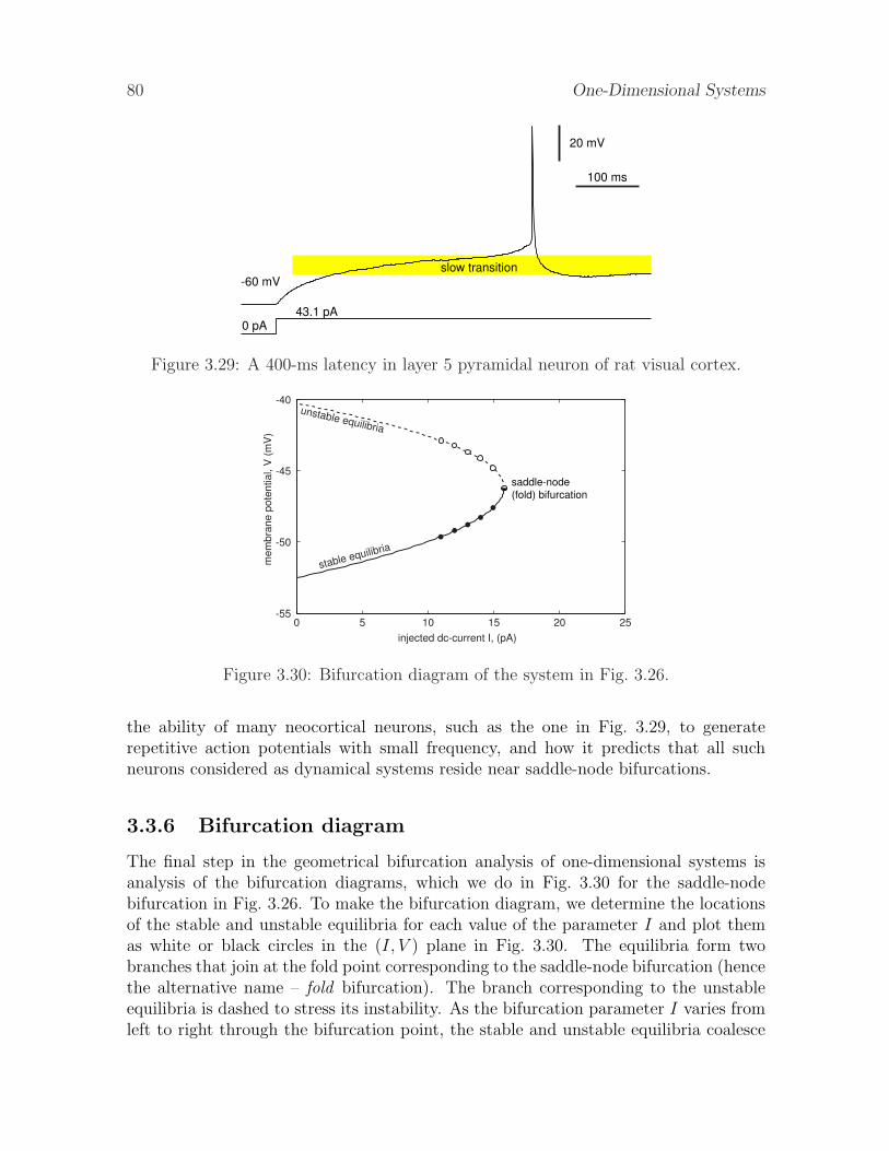
Figure 3.29: A 400-ms latency in layer 5 pyramidal neuron of rat visual cortex.
0 5 10 15 20 25-55
-50
-45
-40
mem
bran
e po
tent
ial,
V (m
V)
injected dc-current I, (pA)
stable equilibria
unstable equilibria
saddle-node (fold) bifurcation
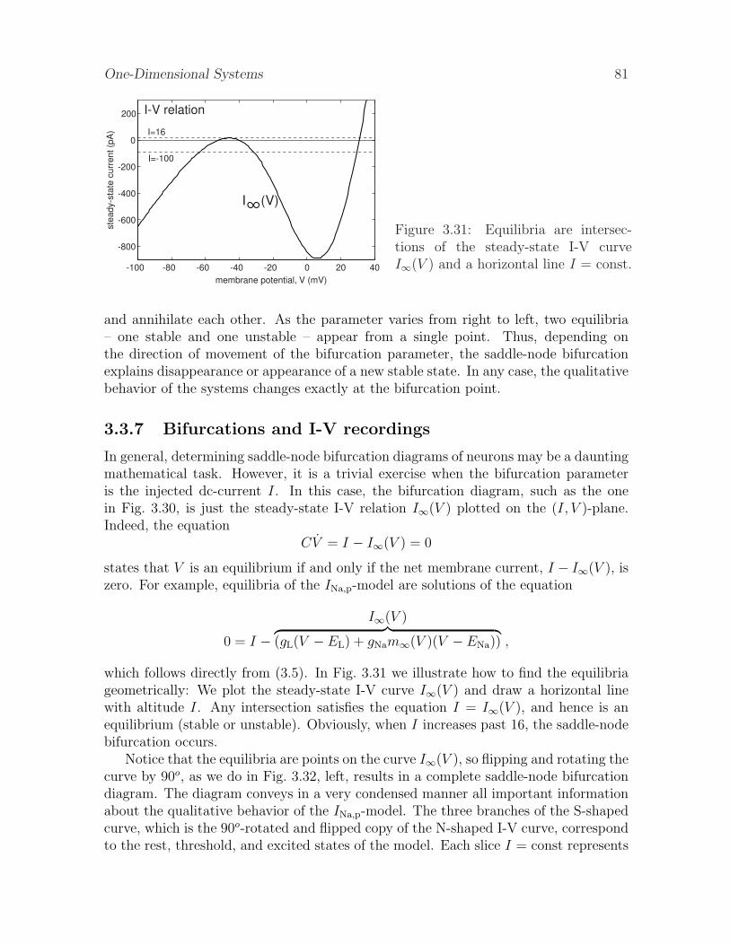
Figure 3.30: Bifurcation diagram of the system in Fig. 3.26.
the ability of many neocortical neurons, such as the one in Fig. 3.29, to generaterepetitive action potentials with small frequency, and how it predicts that all suchneurons considered as dynamical systems reside near saddle-node bifurcations.
3.3.6 Bifurcation diagram
The final step in the geometrical bifurcation analysis of one-dimensional systems isanalysis of the bifurcation diagrams, which we do in Fig. 3.30 for the saddle-nodebifurcation in Fig. 3.26. To make the bifurcation diagram, we determine the locationsof the stable and unstable equilibria for each value of the parameter I and plot themas white or black circles in the (I, V ) plane in Fig. 3.30. The equilibria form twobranches that join at the fold point corresponding to the saddle-node bifurcation (hencethe alternative name – fold bifurcation). The branch corresponding to the unstableequilibria is dashed to stress its instability. As the bifurcation parameter I varies fromleft to right through the bifurcation point, the stable and unstable equilibria coalesce
One-Dimensional Systems 81
-100 -80 -60 -40 -20 0 20 40
-800
-600
-400
-200
0
200
membrane potential, V (mV)
stea
dy-s
tate
cur
rent
(pA
)
I (V)
I-V relation
I=16
I=-100
Figure 3.31: Equilibria are intersec-tions of the steady-state I-V curveI∞(V ) and a horizontal line I = const.
and annihilate each other. As the parameter varies from right to left, two equilibria– one stable and one unstable – appear from a single point. Thus, depending onthe direction of movement of the bifurcation parameter, the saddle-node bifurcationexplains disappearance or appearance of a new stable state. In any case, the qualitativebehavior of the systems changes exactly at the bifurcation point.
3.3.7 Bifurcations and I-V recordings
In general, determining saddle-node bifurcation diagrams of neurons may be a dauntingmathematical task. However, it is a trivial exercise when the bifurcation parameteris the injected dc-current I. In this case, the bifurcation diagram, such as the onein Fig. 3.30, is just the steady-state I-V relation I∞(V ) plotted on the (I, V )-plane.Indeed, the equation
CV = I − I∞(V ) = 0
states that V is an equilibrium if and only if the net membrane current, I − I∞(V ), iszero. For example, equilibria of the INa,p-model are solutions of the equation
0 = I −I∞(V )︷ ︸︸ ︷
(gL(V − EL) + gNam∞(V )(V − ENa)) ,
which follows directly from (3.5). In Fig. 3.31 we illustrate how to find the equilibriageometrically: We plot the steady-state I-V curve I∞(V ) and draw a horizontal linewith altitude I. Any intersection satisfies the equation I = I∞(V ), and hence is anequilibrium (stable or unstable). Obviously, when I increases past 16, the saddle-nodebifurcation occurs.
Notice that the equilibria are points on the curve I∞(V ), so flipping and rotating thecurve by 90o, as we do in Fig. 3.32, left, results in a complete saddle-node bifurcationdiagram. The diagram conveys in a very condensed manner all important informationabout the qualitative behavior of the INa,p-model. The three branches of the S-shapedcurve, which is the 90o-rotated and flipped copy of the N-shaped I-V curve, correspondto the rest, threshold, and excited states of the model. Each slice I = const represents

82 One-Dimensional Systems
-1000 -500 0
-120
-100
-80
-60
-40
-20
0
20
40
injected dc-current, I (pA)
mem
bran
e po
tent
ial,
V (m
V)
-1000 -500 0
-120
-100
-80
-60
-40
-20
0
20
40
injected dc-current, I (pA)
mem
bran
e po
tent
ial,
V (m
V)
rest states
excited states
threshold states
saddle-node (fold) bifurcation
saddle-node (fold) bifurcation
16
-890
I (V)
Figure 3.32: Bifurcation diagram of the INa,p-model (3.5).
the phase portrait of the system, as we illustrate in Fig. 3.32, right. Each point wherethe branches fold (max or min of I∞(V )) corresponds to the saddle-node bifurcation.Since there are two such folds, at I = 16 pA and at I = −890 pA, there are two saddle-node bifurcations in the system. The first one studied in Fig. 3.25 corresponds to thedisappearance of the rest state. The other one illustrated in Fig. 3.33 corresponds tothe disappearance of the excited state. It occurs because I becomes so negative thatthe Na+ inward current is no longer enough to balance the leak outward current andthe negative injected dc-current to keep the membrane in the depolarized (excited)state.
Below the reader can find more examples of bifurcation analysis of the INa,p- andIKir-models, which have non-monotonic I-V relations and can exhibit multi-stability ofstates. The IK- and Ih-models have monotonic I-V relations and hence only one state.These models cannot have saddle-node bifurcations, as the reader is asked to prove inEx. 14 and 15.
3.3.8 Quadratic integrate-and-fire neuron
Let us consider the topological normal form for the saddle-node bifurcation (3.9). From0 = I + V 2 we find that there are two equilibria, Vrest = −
√|I| and Vthresh = +
√|I|
when I < 0. The equilibria approach and annihilate each other via saddle-node bifur-cation when I = 0, so there are no equilibria when I > 0. In this case, V ≥ I and V (t)increases to infinity. Because of the quadratic term, the rate of increase also increases,resulting in a positive feedback loop corresponding to the regenerative activation ofNa+ current. In Ex. 16 we show that V (t) escapes to infinity in a finite time, whichcorresponds to the up-stroke of the action potential. The same up-stroke is generatedwhen I < 0, if the voltage variable is pushed beyond the threshold value Vthresh.

One-Dimensional Systems 83
0
0
0
Bistability
Bifurcation
Monostability
mem
bran
e po
tent
ial,
V
membrane potential, V time
V(t)
Threshold
Rest
Excited
V(t)
Rest
V(t)
Rest
F(V)
Rest
Threshold
Excited
Tangent Point
Rest
Rest
F(V)
F(V)
I=-400
I=-890
I=-1000
mem
bran
e po
tent
ial,
Vm
embr
ane
pote
ntia
l, V
Figure 3.33: Bifurcation in the INa,p-model (3.5): The excited state and the thresholdstate coalesce and disappear when the parameter I is sufficiently small.

84 One-Dimensional Systems
-60 -40 -20
-60
-40
-20
0
20
membrane potential, V (mV)
stea
dy-s
tate
cur
rent
(pA
)
I (V)
I-V relation
(Vsn, Isn)
Isn-k(V-Vsn)2
Figure 3.34: Magnification of the I-V curve in Fig. 3.31 at the left knee shows that itcan be approximated by a square parabola.
Considering infinite values of the membrane potential may be convenient from apurely mathematical point of view, but this has no physical meaning and no way tosimulate it on a digital computer. Instead, we fix a sufficiently large constant Vpeak
and say that (3.9) generated a spike when V (t) reached Vpeak. After the peak of thespike is reached, we reset V (t) to a new value Vreset. The topological normal form forthe saddle-node bifurcation with the after-spike resetting
V = I + V 2 , if V ≥ Vpeak, then V ← Vreset (3.10)
is called the quadratic integrate-and-fire neuron. It is the simplest model of a spikingneuron. The name stems from its resemblance to the leaky integrate-and-fire neuronV = I−V considered in Chap. 8. In contrast to the common folklore, the leaky neuronis not a spiking model because it does not have a spike-generation mechanism, i.e., aregenerative up-stroke of the membrane potential, whereas the quadratic neuron does.We discuss this and other issues in detail in Chap. 8.
In general, quadratic integrate-and-fire model could be derived directly from theequation CV = I − I∞(V ) by approximating the steady-state I-V curve near theresting state by the square parabola I∞(V ) ≈ Isn − k(V − Vsn)
2, where k > 0 andthe peak of the curve (Vsn, Isn) could be easily found experimentally; see Fig. 3.34.Approximating the I-V curve by other functions, for example I∞(V ) = gleak(V −Vrest)−kepV , results in other forms of the model, e.g., the exponential integrate-and-fire model(Fourcaud-Trocme et al. 2003), which has certain advantages over the quadratic form.Unfortunately, the model is not solvable analytically, and it is expensive to simulate.The form I∞(V ) = gleak(V −Vleak)−k(V −Vth)
2+, where x+ = x when x > 0 and x+ = 0
otherwise, combines the advantages of both models. The parameters Vpeak and Vreset
are derived from the shape of the spike. Normalization of variables and parametersresults in the form (3.10) with Vpeak = 1.
In Fig. 3.35 we simulated the quadratic integrate-and-fire neuron to illustrate a

One-Dimensional Systems 85
0
0
0
0
I+V2
I+V2
I<0
I>0
Vreset
Vreset
input
mem
bran
e po
tent
ial,
Vm
embr
ane
pote
ntia
l, V
restthreshold
restthreshold
0
0
0
I+V2
I<0
timemembrane potential, v
Vresetinput
mem
bran
e po
tent
ial,
V
rest Vreset
Vreset
Vreset
rese
tre
set
rese
t
Vpeak
Vpeak
Vpeakbistability
excitability
Figure 3.35: Quadratic integrate-and-fire neuron (3.10) with time-dependent input.
number of its features, which will be described in detail in subsequent chapters usingconductance-based models. First, the neuron is an integrator; each input pulse inFig. 3.35, top, pushes V closer to the threshold value; the higher the frequency of theinput, the sooner V reaches the threshold and starts the up-stroke of a spike. Theneuron is monostable when Vreset ≤ 0 and could be bistable otherwise. Indeed, thefirst spike in Fig. 3.35, middle, is evoked by the input, but the subsequent spikes occurbecause the reset value is superthreshold.
The neuron could be Class 1 or Class 2 excitable depending on the sign of Vreset.Suppose the injected current I slowly ramps up from a negative to a positive value.The membrane potential follows the resting state −
√|I| in a quasi-static fashion until
the bifurcation point I = 0 is reached. At this moment, the neuron starts to fire tonicspikes. In the monostable case Vreset < 0 in Fig. 3.35, bottom, the membrane potential isreset to the left of the ghost of the saddle-node point (see Sect. 3.3.5), thereby producingspiking with an arbitrary small frequency and hence Class 1 excitability. Because of therecurrence, such a bifurcation is called saddle-node on invariant circle. Many pyramidalneurons in mammalian neocortex exhibit such a bifurcation. In contrast, in the bistablecase Vreset > 0, not shown in the figure, the membrane potential is reset to the right ofthe ghost, no slow transition is involved, and the tonic spiking starts with a non-zerofrequency. As an exercise, explain why there is a noticeable latency (delay) to the first
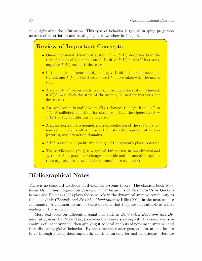
86 One-Dimensional Systems
spike right after the bifurcation. This type of behavior is typical in spiny projectionneurons of neostriatum and basal ganglia, as we show in Chap. 8.
Review of Important Concepts
• One-dimensional dynamical system V = F (V ) describes how therate of change of V depends on V . Positive F (V ) means V increases,negative F (V ) means V decreases.
• In the context of neuronal dynamics, V is often the membrane po-tential, and F (V ) is the steady-state I-V curve taken with the minussign.
• A zero of F (V ) corresponds to an equilibrium of the system. (Indeed,if F (V ) = 0, then the state of the system, V , neither increases nordecreases.)
• An equilibrium is stable when F (V ) changes the sign from “+” to“-”. A sufficient condition for stability is that the eigenvalue λ =F ′(V ) at the equilibrium be negative.
• A phase portrait is a geometrical representation of the system’s dy-namics. It depicts all equilibria, their stability, representative tra-jectories, and attraction domains.
• A bifurcation is a qualitative change of the system’s phase portrait.
• The saddle-node (fold) is a typical bifurcation in one-dimensionalsystems: As a parameter changes, a stable and an unstable equilib-rium approach, coalesce, and then annihilate each other.
Bibliographical Notes
There is no standard textbook on dynamical systems theory. The classical book Non-linear Oscillations, Dynamical Systems, and Bifurcations of Vector Fields by Gucken-heimer and Holmes (1983) plays the same role in the dynamical systems community asthe book Ionic Channels and Excitable Membranes by Hille (2001) in the neurosciencecommunity. A common feature of these books is that they are not suitable as a firstreading on the subject.
Most textbooks on differential equations, such as Differential Equations and Dy-namical Systems by Perko (1996), develop the theory starting with the comprehensiveanalysis of linear systems, then applying it to local analysis of non-linear systems, andthen discussing global behavior. By the time the reader gets to bifurcations, he hasto go through a lot of daunting math, which is fun only for mathematicians. Here we

One-Dimensional Systems 87
follow approach similar to Nonlinear Dynamics and Chaos by Strogatz (1994): Insteadof going from linear to non-linear systems, we go from one-dimensional non-linear sys-tems (this chapter) to two-dimensional non-linear systems (next chapter). Instead ofproviding the theory with a lot of mathematics, we use the geometrical approach toprovoke the reader’s intuition. (There is plenty of fun math in exercises and in thelater chapters.)
Exercises
1. Consider a neuron having Na+ current with fast activation kinetics. Assume thatinactivation of this current, as well as (in)activations of the other currents in theneuron are much slower. Prove that the initial segment of action potential up-stroke of this neuron can be approximated by the INa,p-model (3.5). Use Fig. 3.15to discuss the applicability of this approximation.
2. Draw phase portraits of the systems in Fig. 3.36. Clearly mark all equilibria,their stability, attraction domains, and direction of trajectories. Determine thesigns of eigenvalues at each equilibrium.
F(V) F(V) F(V)
V V V
a b c
Figure 3.36: Draw phase portrait of the system V = F (V ) with shown F (V ).
3. Draw phase portraits of the following systems
(a) x = −1 + x2
(b) x = x− x3
Determine the eigenvalues at each equilibrium.
4. Determine stability of the equilibrium x = 0 and draw phase portraits of thefollowing piece-wise continuous systems
(a) x =
{2x, if x < 0x, if x ≥ 0
(b) x =
−1, if x < 0
0, if x = 01, if x > 0
(c) x =
{ −2/x, if x 6= 00, if x = 0

88 One-Dimensional Systems
F (V)1
V
a
V
F (V)2
V
b
V
F (V)2
F (V)1
F (V)1
V
c
V
F (V)2
V
d
V
F (V)2
F (V)1F (V)1
V
e
V
F (V)2V
f
V
F (V)2
F (V)1
Figure 3.37: Which of the pairs correspond to topologically equivalent dynamical sys-tems? (All intersections with the V axis are marked as dots.)
5. Draw phase portraits of the systems in Fig. 3.37. Which of the pairs in the figurecorrespond to topologically equivalent dynamical systems?
6. (Saddle-node bifurcation) Draw bifurcation diagram and representative phaseportraits of the system x = a + x2, where a is a bifurcation parameter. Find theeigenvalues at each equilibrium.
7. (Saddle-node bifurcation) Use definition in Sect. 3.3.4 to find saddle-node bifur-cation points in the following systems:
(a) x = a + 2x + x2
(b) x = a + x + x2
(c) x = a− x + x2
(d) x = a− x + x3 (Hint: verify the non-hyperbolicity condition first)
(e) x = 1 + ax + x2
(f) x = 1 + 2x + ax2
where a is the bifurcation parameter.
8. (Pitchfork bifurcation) Draw bifurcation diagram and representative phase por-traits of the system x = bx − x3, where b is a bifurcation parameter. Find theeigenvalues at each equilibrium.

One-Dimensional Systems 89
-140 -70 00
0.2
0.4
0.6
0.8
1
Membrane Voltage (mV)
h (V)
-100 -50 0-2
-1
0
1
2
Membrane Voltage (mV)
F(V)
I (V)Kir
Cur
rent
EK-100
-80
-60
-40
-20
0
20
-140 -70 0Membrane Voltage (mV)
I (V)L
EL
Figure 3.38: The IKir-model having injected current (I), leak current (IL), and instan-taneous K+ inward rectifier current (IKir) and described by (3.11). Inactivation curveh∞(V ) is modified from Wessel et. al (1999). Parameters: C = 1, I = 6, gL = 0.2,EL = −50, gKir = 2, EK = −80, V1/2 = −76, k = −12 (see Fig. 2.20).
-100 -50 0 50 1000
0.2
0.4
0.6
0.8
1
-100 -50 0 50 100-150
-100
-50
0
50
100
I (V)Na,p
Membrane Voltage (mV)Membrane Voltage (mV)
Cur
rent
m (V)
ENaEL
I (V)L
Membrane Voltage (mV)
F(V)
-100 -50 0 50 100-50
0
50
Figure 3.39: The INa,p-model having leak current (IL) and persistent Na+ current(INa,p) and described by (3.5) with the right-hand side function F (V ). Parameters:C = 1, I = 0, gL = 1, EL = −80, gNa = 2.25, ENa = 60, V1/2 = −20, k = 15 (seeFig. 2.20).
9. Draw bifurcation diagram of the IKir-model
C V = I − gL(V − EL)−instantaneous IKir︷ ︸︸ ︷
gKirh∞(V )(V − EK) , (3.11)
using parameters from Fig. 3.38 and treating I as a bifurcation parameter.
10. Derive an explicit formula that relates the position of the equilibrium in theHodgkin-Huxley model to the magnitude of the injected dc-current I. Are thereany saddle-node bifurcations?
11. Draw bifurcation diagram of the INa,p-model (3.5) using parameters from Fig. 3.39and treating
(a) gL as a bifurcation parameter,
(b) EL as a bifurcation parameter.

90 One-Dimensional Systems
I (V)K
Membrane Voltage (mV)Membrane Voltage (mV)
Cur
rent
m (V)
EK EL
I (V)L
-120 -100 -80 -60 -40 -20 00
0.2
0.4
0.6
0.8
1
-120 -100 -80 -60 -40 -20 0-50
0
50
100
-120 -100 -80 -60 -40 -20 0-50
0
50
Membrane Voltage (mV)
F(V)
Figure 3.40: The IK-model having leak current (IL) and persistent K+ current (IK)and described by (3.12). Parameters: C = 1, gL = 1, EL = −80, gK = 1, EK = −90,V1/2 = −53, k = 15 (see Fig. 2.20).
I (V)h
Membrane Voltage (mV)Membrane Voltage (mV)
Cur
rent
h (V)
EhEL
I (V)L
-120 -100 -80 -60 -40 -20 00
0.2
0.4
0.6
0.8
1
-120 -100 -80 -60 -40 -20 0-100
-50
0
50
-120 -100 -80 -60 -40 -20 0-100
-50
0
50
100
Membrane Voltage (mV)
F(V)
Figure 3.41: The Ih-model having leak current (IL) and “hyperpolarization-activated”inward current Ih and described by (3.13). Parameters: C = 1, gL = 1, EL = −80,gh = 1, Eh = −43, V1/2 = −75, k = −5.5 (Huguenard and McCormick 1992).
12. Draw bifurcation diagram of the IKir-model (3.11) using parameters from Fig. 3.38and treating
(a) gL as a bifurcation parameter,
(b) gKir as a bifurcation parameter.
13. Perform the bifurcation analysis of the INa,p-model with I = 0 and gNa as abifurcation parameter. In particular, use computer simulations to reproduceanalogues of figures 3.25, 3.26, and 3.30–3.33.
14. Show that the IK-model in Fig. 3.40
C V = −gL(V − EL)−instantaneous IK︷ ︸︸ ︷
gKm4∞(V )(V − EK) . (3.12)
cannot exhibit saddle-node bifurcation for V > EK. (Hint: show that F ′(V ) 6= 0for all V > EK.)

One-Dimensional Systems 91
15. Show that the Ih-model in Fig. 3.41
C V = −gL(V − EL)−instantaneous Ih︷ ︸︸ ︷
ghh∞(V )(V − Eh) (3.13)
cannot exhibit saddle-node bifurcation for any V < Eh.
16. Prove that the upstroke of the spike in the quadratic integrate-and-fire neuron(3.9) has the asymptote 1/(c− t) for some c > 0.
17. (Cusp bifurcation) Draw bifurcation diagram and representativephase portraits of the system x = a + bx − x3, where a and b are bifurcationparameters. Plot the bifurcation diagram in the (a, b, x)-space and on the (a, b)-plane.
18. (Gradient systems) An n-dimensional dynamical system x = f(x), x = (x1, . . . , xn) ∈Rn is said to be gradient when there is a potential (energy) function E(x) suchthat
x = − grad E(x) ,
wheregrad E(x) = (Ex1 , . . . , Exn)
is the gradient of E(x). Show that all one-dimensional systems are gradient (Hint:see Fig. 3.11). Find potential (energy) functions for the following one-dimensionalsystems
a. V = 0 b. V = 1 c. V = −V
d. V = −1 + V 2 e. V = V − V 3 f. V = − sin V
19. Consider a dynamical system x = f(x) , x(0) = x0.
(a) (Stability) An equilibrium y is stable if any solution x(t) with x0 sufficientlyclose to y remains near y for all time. That is, for all ε > 0 there existsδ > 0 such that if |x0 − y| < δ then |x(t)− y| < ε for all t ≥ 0.
(b) (Asymptotic stability) A stable equilibrium y is asymptotically stable if allsolutions starting sufficiently close to y approach it as t → ∞. That is, ifδ > 0 from the definition above could be chosen so that limt→∞ x(t) = y.
(c) (Exponential stability) A stable equilibrium y is said to be exponentiallystable when there is a constant a > 0 such that |x(t)− y| < exp(−at) for allx0 near y and all t ≥ 0.
Prove that (c) implies (b), and (b) implies (a). Show that (a) does not imply(b) and (b) does not imply (c); That is, present a system having stable but notasymptotically stable equilibrium, and a system having asymptotically but notexponentially stable equilibrium.