1

Cha

pter

3Laplace Transforms

• Important analytical method for solving linear ordinarydifferential equations.

- Application to nonlinear ODEs? Must linearize first.

• Laplace transforms play a key role in important process control concepts and techniques.

- Examples:

• Transfer functions

• Frequency response

• Control system design

• Stability analysis

2

Cha

pter

3Definition

The Laplace transform of a function, f(t), is defined as

[ ] ( )0

( ) ( ) (3-1)stF s f t f t e dt∞ −= = ∫L

where F(s) is the symbol for the Laplace transform, L is the Laplace transform operator, and f(t) is some function of time, t.

Note: The L operator transforms a time domain function f(t) into an s domain function, F(s). s is a complex variable: s = a + bj, 1j −

3

Cha

pter

3Inverse Laplace Transform, L-1:

By definition, the inverse Laplace transform operator, L-1, converts an s-domain function back to the corresponding time domain function:

( ) ( )1f t F s− = L

Important Properties:

Both L and L-1 are linear operators. Thus,

( ) ( ) ( ) ( )( ) ( ) (3-3)

ax t by t a x t b y t

aX s bY s

+ = + = +

L L L

4

Cha

pter

3where:

- x(t) and y(t) are arbitrary functions

- a and b are constants

- ( ) ( ) ( ) ( )X s x t Y s y t L Land

Similarly,

( ) ( ) ( ) ( )1 aX s bY s ax t b y t− + = + L

5

Cha

pter

3Laplace Transforms of Common Functions

1. Constant Function

Let f(t) = a (a constant). Then from the definition of the Laplace transform in (3-1),

( )0

0

0 (3-4)st sta a aa ae dt es s s

∞∞ − − = = − = − − =

∫L

6

Cha

pter

32. Step Function

The unit step function is widely used in the analysis of processcontrol problems. It is defined as:

( )0 for 0

(3-5)1 for 0

tS t

t<

≥

Because the step function is a special case of a “constant”, it follows from (3-4) that

( ) 1 (3-6)S ts

= L

7

Cha

pter

33. Derivatives

This is a very important transform because derivatives appear in the ODEs we wish to solve. In the text (p.53), it is shown that

( ) ( )0 (3-9)df sF s fdt

= − L

initial condition at t = 0

Similarly, for higher order derivatives:

( ) ( ) ( ) ( )

( ) ( ) ( ) ( )

11 2

2 1

0 0

... 0 0 (3-14)

nn n n

n

n n

d f s F s s f s fdt

sf f

− −

− −

= − − −

− − −

L

8

Cha

pter

3where:

- n is an arbitrary positive integer

- ( ) ( )0

0k

kk

t

d ffdt =

Special Case: All Initial Conditions are Zero

Suppose Then( )

In process control problems, we usually assume zero initial conditions. Reason: This corresponds to the nominal steady state when “deviation variables” are used, as shown in Ch. 4.

( ) ( )0 0 ... 0 .f f f= = =( ) ( )1 1n−

( )n

nn

d f s F sdt

=

L

9

Cha

pter

34. Exponential Functions

Consider where b > 0. Then, ( ) btf t e−=

( )

( )

0 0

0

1 1 (3-16)

b s tbt bt st

b s t

e e e dt e dt

eb s s b

∞ ∞ − +− − −

∞− +

= =

= − = + +

∫ ∫L

5. Rectangular Pulse Function

It is defined by:

( )0 for 0

for 0 (3-20)0 for

w

w

tf t h t t

t t

<= ≤ < ≥

10

Cha

pter

3

h

( )f t

wtTime, t

The Laplace transform of the rectangular pulse is given by

( ) ( )1 (3-22)wt shF s es

−= −

11

Cha

pter

36. Impulse Function (or Dirac Delta Function)The impulse function is obtained by taking the limit of therectangular pulse as its width, tw, goes to zero but holdingthe area under the pulse constant at one. (i.e., let )

Let,

Then,

1

wh

t=

( )tδ impulse function

( ) 1tδ = L

Solution of ODEs by Laplace TransformsProcedure:1. Take the L of both sides of the ODE.

2. Rearrange the resulting algebraic equation in the s domain to solve for the L of the output variable, e.g., Y(s).

3. Perform a partial fraction expansion.4. Use the L-1 to find y(t) from the expression for Y(s).

12

Cha

pter

3Table 3.1. Laplace Transforms

See page 54 of the text.

13

Cha

pter

3Example 3.1Solve the ODE,

( )5 4 2 0 1 (3-26)dy y ydt

+ = =

First, take L of both sides of (3-26),

( )( ) ( ) 25 1 4sY s Y ss

− + =

Rearrange,

( ) ( )5 2 (3-34)5 4sY s

s s+

=+

Take L-1,( ) ( )

1 5 25 4sy t

s s− +

= + L

From Table 3.1,

( ) 0.80.5 0.5 (3-37)ty t e−= +

14

Cha

pter

3Partial Fraction Expansions

Basic idea: Expand a complex expression for Y(s) into simpler terms, each of which appears in the LaplaceTransform table. Then you can take the L-1 of both sides of the equation to obtain y(t).

Example:

( ) ( )( )5 (3-41)

1 4sY s

s s+

=+ +

Perform a partial fraction expansion (PFE)

( )( )1 25 (3-42)

1 4 1 4s

s s s sα α+

= ++ + + +

where coefficients and have to be determined.1α 2α

15

Cha

pter

3To find : Multiply both sides by s + 1 and let s = -11α

11

5 44 3s

ss

α=−

+∴ = =

+

To find : Multiply both sides by s + 4 and let s = -42α

24

5 11 3s

ss

α=−

+∴ = = −

+

A General PFEConsider a general expression,

( ) ( )( )

( )

( )1

(3-46a)ni

i

N s N sY s

D s s bπ=

= =+

16

Cha

pter

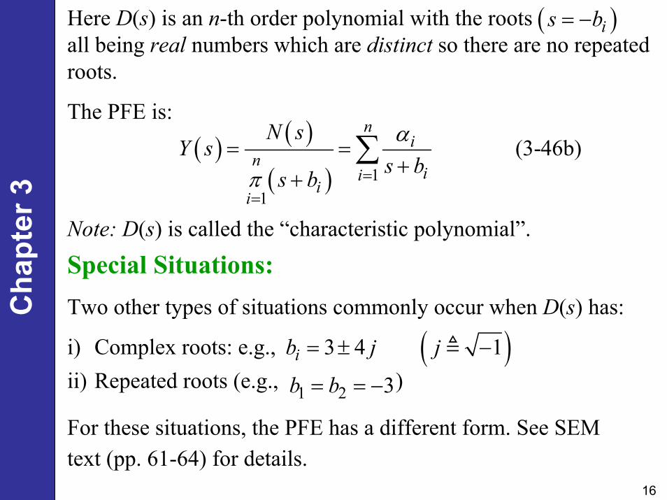
3Here D(s) is an n-th order polynomial with the roots all being real numbers which are distinct so there are no repeated roots.

The PFE is:

( )is b= −

( ) ( )

( ) 11

(3-46b)n

in

iii

i

N sY s

s bs b

α

π ==

= =+

+∑

Note: D(s) is called the “characteristic polynomial”.

Special Situations:Two other types of situations commonly occur when D(s) has:

i) Complex roots: e.g., ii) Repeated roots (e.g., )

For these situations, the PFE has a different form. See SEMtext (pp. 61-64) for details.

3b b= = −( )3 4 1ib j j= ± −

1 2

17

Cha

pter

3Example 3.2 (continued)

Recall that the ODE, , with zero initial conditions resulted in the expression

6 11 6 1y y y y+ + + + =

( ) ( )3 21 (3-40)

6 11 6Y s

s s s s=

+ + +

The denominator can be factored as

( ) ( )( )( )3 26 11 6 1 2 3 (3-50)s s s s s s s s+ + + = + + +

Note: Normally, numerical techniques are required in order to calculate the roots.

The PFE for (3-40) is

( ) ( )( )( )31 2 41 (3-51)

1 2 3 1 2 3Y s

s s s s s s s sαα α α

= = + + ++ + + + + +

18

Cha

pter

3Solve for coefficients to get

1 2 3 41 1 1 1, , ,6 2 2 6

α α α α= = − = = −

(For example, find , by multiplying both sides by s and then setting s = 0.)

α

Substitute numerical values into (3-51):1/ 6 1/ 2 1/ 2 1/ 6( )

1 2 3Y s

s s s s= − + +

+ + +

Take L-1 of both sides:

( )1 1 1 1 11/ 6 1/ 2 1/ 2 1/ 61 2 3

Y ss s s s

− − − − − = − + + + + + L L L L L

From Table 3.1,

( ) 2 31 1 1 1 (3-52)6 2 2 6

t t ty t e e e− − −= − + −

19

Cha

pter

3Important Properties of Laplace Transforms

1. Final Value Theorem

It can be used to find the steady-state value of a closed loop system (providing that a steady-state value exists.

Statement of FVT:

( ) ( )0

limlimt s

sY sy t→∞ →

=

providing that the limit exists (is finite) for all where Re (s) denotes the real part of complex

variable, s. ( )Re 0,s ≥

20

Cha

pter

3Example:

Suppose,

( ) ( )5 2 (3-34)5 4sY s

s s+

=+

Then,

( ) ( )0

5 2lim 0.5lim 5 4t s

sy y ts→∞ →

+ ∞ = = = +

2. Time Delay

Time delays occur due to fluid flow, time required to do an analysis (e.g., gas chromatograph). The delayed signal can be represented as

( )θ θ time delayy t − =Also,

( ) ( )θθ sy t e Y s− − = L