Embed Size (px)
Citation preview
47
CHAPTER 3
THEORETICAL BACKGROUND
3.1 GENERAL
Natural Language Processing (NLP) research has a long tradition in European
countries. It has taken giant leaps in the last decade with the initiation of efficient
machine learning algorithms and the creation of large annotated corpora for various
languages. In countries like India where more than thousands of language are in usage,
so, the importance of the NLP is very relevant. However, NLP research in Indian
languages has mainly focused on the development of rule based techniques due to the
lack of annotated corpora. The pre-requisites for developing NLP applications in Tamil
language are the availability of speech corpora, annotated text corpora, parallel corpora,
lexical resources and computational models. The sparseness of these resources for
Tamil language is one of the major reasons for the slow growth of NLP work in Tamil.
Like other language processing, Tamil language also involves morphological analysis,
syntax analysis and semantic analysis.
3.1.1 Tamil Language
Tamil belongs to the southern branch of the Dravidian languages, a family of around
twenty-six languages native to the Indian subcontinent. It flourished in India as a
language with rich literature during the Sangam period (300 BCE to 300 CE). Tamil
scholars categorize the history of the language into three periods, Old Tamil (300 BC -
700 CE), Middle Tamil (700 - 1600) and Modern Tamil (1600–present). In Old Tamil,
Epigraphic attestation of Tamil begins with rock inscriptions from the 3rd century BC,
written in Tamil-Brahmi, an adapted form of the Brahmi script. The earliest extant
literary text is the ெதால்காப்பியம் (tholkAppiyam), a work on grammar and poetics
which describes the language of the classical period. The Sangam literature contains
about 50,000 lines of poetry contained in 2381 poems attributed to 473 poets including
many women poets [9].
During Modern Tamil i.e., in the early 20th century, the chaste Tamil
Movement called for the removal of all Sanskrit and other foreign elements from
48
Tamil. It received support from Dravidian parties and nationalists who supported Tamil
independence. This led to the replacement of a significant number of Sanskrit loan
words by Tamil equivalents. An important factor specific to Tamil is the existence of
two main varieties of the language, colloquial and formal Tamil ெசந்தமிழ்
(sewthamiz), which are sufficiently divergent that the language is classed as diglossic.
Colloquial Tamil is used for most spoken communication, and formal Tamil is spoken
in a restricted number of high contexts, such as lectures and news bulletins, and also
used in writing. They differ in terms of their lexis, morphology, and segmental
phonology.
Tamil is the official language of the Indian state of Tamilnadu and one of the 22
languages under schedule 8 of the constitution of India. It is also one of the official
languages of the Union Territories of Puducherry, Andaman & Nicobar Islands, Sri
Lanka, Malaysia and Singapore. Tamil became the first legally recognized classical
language of India in the year 2004 [9].
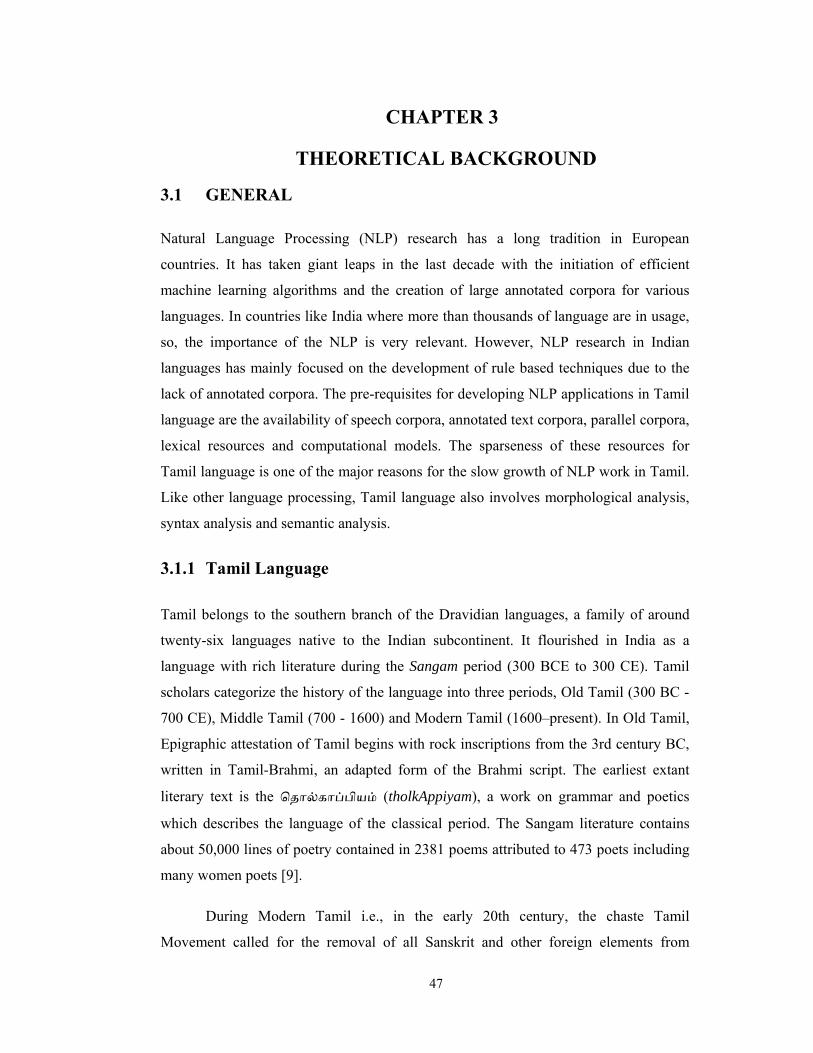
3.1.2 Tamil Grammar
Traditional Tamil grammar consists of five parts, namely எ த் (ezuththu), ெசால்
(sol), ெபா ள் (poruL), யாப் (yAppu) and அணி(aNi). Of these, the last two are
applicable mostly in poetry. The following Table 3.1 gives additional information about
these parts. The tholkAppiyam (ெதால்காப்பியம்) is the oldest work on the grammar of
the Tamil language [132].
Table 3.1 Tamil Grammar
Divisions Meaning Main grammar books
எ த் (Ezuththu ) Letter ெதால்காப்பியம்(tholkAppiyam),நன் ல் (wannUl)
ெசால் (sol) Word ெதால்காப்பியம்(tholkAppiyam),நன் ல் (wannUl)
ெபா ள் (poruL) Meaning ெதால்காப்பியம் (tholkAppiyam)
யாப் (yAppu) Form யாப்ெப ம்கலாக்காாிைக(yApperungkalAkkArikai )
அணி (aNi) Method தனியலங்காரம் (thaniyalangkAram)
49
3.1.3 Tamil Characters
Tamil is written using a script called the vattEzuththu. The Tamil script has twelve
vowels uyirezuththu (உயிெர த் ) "soul-letters", eighteen consonants meyyezuththu
(ெமய்ெய த் ) "body-letters" and one character, the Aythaezuththu (ஆய்த எ த் )
“the hermaphrodite letter”, which is classified in Tamil grammar as being neither a
consonant nor a vowel though often considered as part of the vowel set. The script,
however, is syllabic and not alphabetic.
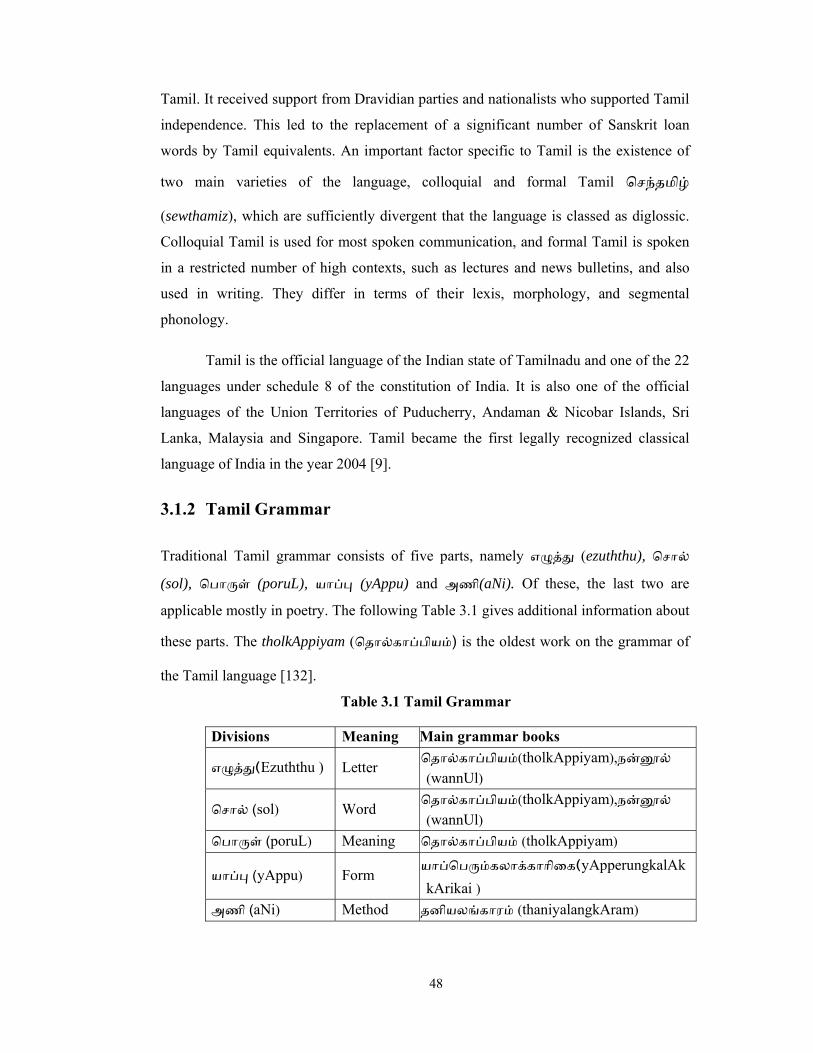
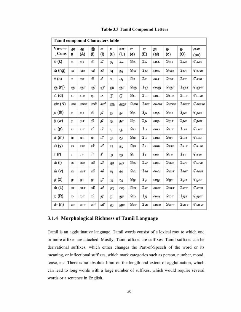
The complete script, therefore, consists of the thirty-one letters in their independent
form, and an additional 216 compound letters representing a total 247 combinations.
These compound letters are formed by adding a vowel marker to the consonant. The
details of Tamil vowels are given in Table 3.2. Some vowels require the basic shape of
the consonant to be altered in a way that is specific to that vowel. Others are written by
adding a vowel-specific suffix to the consonant, yet others a prefix, and finally some
vowels require adding both a prefix and a suffix to the consonant. The following Table
3.3 lists vowel letters across the top and consonant letters along the side, the
combination of which gives all Tamil compound ( uyirmei) letters.
Table 3.2 Tamil Vowels
In every case, the vowel marker is different from the standalone character for the
vowel. The Tamil script is written from left to right. Vowels are also called the 'life'
(uyir) or 'soul' letters. Tamil vowels are divided into short and long kuril and nedil -
five of each type) and two diphthongs. Tamil compound (uyirmei) letters are formed by
adding a vowel marker to the consonant. There are 216 compound letters in Tamil. The
Tamil transliteration is given in the Appendix A.
Short vowel Long vowel Diphthong
அ ஆ ஐ இ ஈ
உ ஊ ஔ எ ஏ
ஒ ஒ
50
Table 3.3 Tamil Compound Letters
Tamil compound Characters table
Vow→ ↓Cons
அ a
ஆ (A)
இ (i)
ஈ (I)
உ (u)
ஊ (U)
எ (e)
ஏ (E)
ஐ (ai)
ஒ (o)
ஓ (O)
ஔ (au)
க் (k) க கா கி கீ கு கூ ெக ேக ைக ெகா ேகா ெகௗ
ங் (ng) ங ஙா ஙி ஙீ ஙு ஙூ ெங ேங ைங ெஙா ேஙா ெஙௗ
ச் (s) ச சா சி சீ சு சூ ெச ேச ைச ெசா ேசா ெசௗ
ஞ் (nj) ஞ ஞா ஞி ஞீ ெஞ ேஞ ைஞ ெஞா ேஞா ெஞௗ
ட் (d) ட டா டீ ெட ேட ைட ெடா ேடா ெடௗ
ண் (N) ண ணா ணி ணீ ெண ேண ைண ெணா ேணா ெணௗ
த் (th) த தா தி தீ ெத ேத ைத ெதா ேதா ெதௗ
ந் (w) ந நா நி நீ ெந ேந ைந ெநா ேநா ெநௗ
ப் (p) ப பா பி பீ ெப ேப ைப ெபா ேபா ெபௗ
ம் (m) ம மா மி மீ ெம ேம ைம ெமா ேமா ெமௗ
ய் (y) ய யா யி யீ ெய ேய ைய ெயா ேயா ெயௗ
ர் (r) ர ரா ாி ாீ ெர ேர ைர ெரா ேரா ெரௗ
ல் (l) ல லா லீ ெல ேல ைல ெலா ேலா ெலௗ
வ் (v) வ வா வி ெவ ேவ ைவ ெவா ேவா ெவௗ
ழ் (z) ழ ழா ழி ழீ ெழ ேழ ைழ ெழா ேழா ெழௗ
ள் (L) ள ளா ளி ளீ ெள ேள ைள ெளா ேளா ெளௗ
ற் (R) ற றா றி றீ ெற ேற ைற ெறா ேறா ெறௗ
ன் (n) ன னா னி னீ ென ேன ைன ெனா ேனா ெனௗ
3.1.4 Morphological Richness of Tamil Language
Tamil is an agglutinative language. Tamil words consist of a lexical root to which one
or more affixes are attached. Mostly, Tamil affixes are suffixes. Tamil suffixes can be
derivational suffixes, which either changes the Part-of-Speech of the word or its
meaning, or inflectional suffixes, which mark categories such as person, number, mood,
tense, etc. There is no absolute limit on the length and extent of agglutination, which
can lead to long words with a large number of suffixes, which would require several
words or a sentence in English.
51
Tamil is a morphologically rich language in which most of the morphemes
coordinate with the root words in the form of suffixes. Suffixes are used to perform the
functions of cases, plural marker, euphonic increment and postpositions in noun class.
Tamil verbs are inflected for tense, person, number, gender, mood and voice. Other
features of Tamil language are, using plural for honorific noun, frequent echo words,
and null subject feature i.e. not all sentences have subject. Computationally, each root
word can take more than ten thousand inflected word-forms, out of which only a few
hundred will exist in a typical corpus [129]. Tamil is consistently head-final language.
The verb comes at the end of the clause with a typical word order of Subject-Object-
Verb (SOV). However, Tamil language allows word order to be changed, making it a
relatively word order free language. In Tamil, subject-verb agreement is required for
the grammaticality of a Tamil sentence.
3.1.5 Challenges in Tamil NLP
There are many issues that make a Tamil language processing task to difficult. These
relate to the problems of representation and interpretation. Language computing
requires precise representation of context. The natural languages are highly ambiguous
and vague, so achieving such representations are very hard. The various sources of
ambiguities in Tamil language are described below.
3.1.5.1 Ambiguity in Morphemes
Tamil morphemes are ambiguous in the grammatical category and the position it takes
in a word construction.
Ambiguity in morpheme’s grammatical category
A morpheme can have more than one grammatical category. For example, the
morpheme athu, ana, thu can occur as Nominalizing suffix or 3rd Person neuter
suffix.
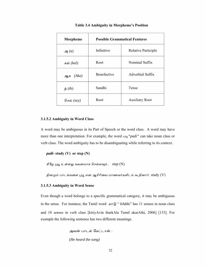
Ambiguity in morpheme’s position
The suffixation of the morpheme’s position also leads to ambiguity. The Table 3.4
gives a few examples for the morphemes and its possible grammatical features.
52
Table 3.4 Ambiguity in Morpheme’s Position
3.1.5.2 Ambiguity in Word Class
A word may be ambiguous in its Part of Speech or the word class. A word may have
more than one interpretation. For example, the word ப “padi” can take noun class or
verb class. The word ambiguity has to be disambiguating while referring to its context.
padi- study (V) or step (N)
கீேழ ப உள்ள கவனமாக ெசல்ல ம் . step (N)
தின ம் பாடங்கைள ப என ஆசிாிைய மாணவர்களிடம் கூறினார். study (V)
3.1.5.3 Ambiguity in Word Sense
Even though a word belongs to a specific grammatical category, it may be ambiguous
in the sense. For instance, the Tamil word கா “ kAddu” has 11 senses in noun class
and 18 senses in verb class [kiriyAvin tharkAla Tamil akarAthi, 2006] [133]. For
example the following sentence has two different meanings.
அவன் பாடல் ேகட்டான் .
(He heard the song)
Morpheme Possible Grammatical Features
அ (a) Infinitive Relative Participle
கல் (kal) Root Nominal Suffix
ஆக (Aka) Benefactive Adverbial Suffix
த் (th) Sandhi Tense
ெசய் (sey) Root Auxiliary Root
53
(He ask the song )
3.1.5.4 Ambiguity in Sentence
A sentence may be ambiguous even if the words are not ambiguous. For example, the
following sentence has two interpretations.
“நான் ஒ அழகான ெபண்ைண ம் ஆைண ம் பார்த்ேதன்”
(I saw the beautiful women and men)
(I saw the beautiful women and beautiful men).
The words are not ambiguous but the sentences are ambiguous.
3.2 MORPHOLOGY
Morphology is the field within linguistics that studies the internal structure of words.
While words are generally accepted as being the smallest units of syntax, it is clear that
in most (if not all) languages, words can be related to other words by rules.
Morphology is the branch of linguistics that studies patterns of word-formation within
and across languages, and attempts to formulate rules that model the knowledge of the
speakers of those languages.
3.2.1 Types of Morphology
Morphology is traditionally classified into three main divisions: inflection, derivation,
and compounding. Inflectional morphology deals with the formation of different forms
in the paradigm of a lexeme. In inflectional morphology, words undergo a change in
their form to express some grammatical functions but their syntactic category remains
unchanged. Many inflectional features appear on words to express agreement purposes
(agreement in person, number, and gender) as well as to express case, aspect, mood,
and tense.
The derivational morphology is concerned with “the creation of a new lexeme
via affixation”. In English, the process of word formation through derivation involves
two types of affixation: prefixation, which means placing a morpheme before a word,
e.g. un-happy; and suffixation, which means placing a morpheme after a word, e.g.
54
happi-ness. Derivation poses a problem to translation in that “not all derived words
have straight-forward compositional translation as derived words. In English, for
example, the same meaning can be expressed by different affixes. Moreover, the same
affix can have more than one meaning. This can be exemplified by the suffix -er. This
suffix can be used to express the agent as in player and singer. But this is not the only
meaning it can convey as it can describe instruments as in mixer and cooker. In this
way the affix can have a range of equivalents in the target language and the attempt to
have one-to-one correspondences for affixes will be greatly misguided.
Compounding morphology is the process of forming a new word through
combining two or more words. Compounding is a process of word formation that
involves combining complete word forms into a single compound form; dog catcher is
therefore a compound, because both dog and catcher are complete word forms in their
own right before the compounding process has been applied, and are subsequently
treated as one form. An important notion in compounding is the notion of head. A
compound noun is divided into head and modifier or modifiers. For instance, the
compound noun watchtower in which watch and tower can be represented as a head
and modifier.
3.2.2 Lexemes
A lexical database is organized around lexemes, which include all the morphemes of a
language. A lexeme is conventionally listed in a dictionary as a separate entry.
Generally lexeme corresponds to a set of forms taken by a single word. For example, in
the English language, run, runs, ran and running are forms of the same lexeme “run”.
3.2.3 Lemma and Stems
A lemma in morphology is the canonical form of a lexeme. In lexicography, this unit is
usually the citation form or headword by which it is indexed. Lemmas have special
significance in highly inflected languages such as Tamil. The process of determining
the lemma for a given word is called lemmatization.
A stem is the part of the word that never changes even when morphologically
inflected, whilst a lemma is the base form of the verb. For example, for the word
"produced", the lemma is "produce", but the stem is “produc-”. This is because there
55
are words such as production. In linguistic analysis, the stem is defined more generally
as the analyzed base form from which all inflected forms can be formed. When
phonology is taken into account, the definition of the unchangeable part of the word is
not useful, as can be seen in the phonological forms of the words in the preceding
example: "produced" vs. "production".
3.2.4 Inflections and Word Forms
Given the notion of a lexeme, it is possible to distinguish two kinds of morphological
rules. Some morphological rules relate different forms of the same lexeme; while other
rules relate two different lexemes. Rules of the first kind are called inflectional rules,
while those of the second kind are called word-formation. The English plural, as
illustrated by dog and dogs, is an inflectional rule; compounds like dog-catcher or
dishwasher provide an example of a word-formation rule. Informally, word-formation
rules form "new words" (that is, new lexemes), while inflection rules yield variant
forms of the "same" word (lexeme).
Derivation involves affixing bound (non-independent) forms to existing lexemes,
whereby the addition of the affix derives a new lexeme. One example of derivation is
clear in this case: the word independent is derived from the word dependent by
prefixing it with the derivational prefix in-, while dependent itself is derived from the
verb depend.
3.2.5 Morphemes and Types
Morpheme is the minimal meaningful unit in a word. The concept of word and
morpheme are different, a morpheme may or may not stand alone. One or several
morphemes compose a word.
• Free morphemes, like town and dog, can appear with other lexemes (as in town
hall or dog house) or they can stand alone, i.e. "free".
• Bound morphemes like "un-" appear only together with other morphemes to
form a lexeme. Bound morphemes in general tend to be prefixes and suffixes.

56
• Derivational morphemes can be added to a word to create (derive) another
word: the addition of "-ness" to "happy," for example, to give "happiness." They
carry semantic information.
• Inflectional morphemes modify a word's tense, number, aspect, and so on,
without deriving a new word or a word in a new grammatical category (as in the
"dog" morpheme if written with the plural marker morpheme "-s" becomes
"dogs"). They carry grammatical information.
Agglutinative languages have words containing several morphemes that are always
clearly differentiable from one another in that each morpheme represents only one
grammatical meaning and the boundaries between those morphemes are easily
demarcated. The bound morphemes are affixes, and they may be individually
identified. Agglutinative languages tend to have a high number of morphemes per
word, and their morphology is highly regular [134].
3.2.6 Allomorphs
One of the largest sources of complexity in morphology is one-to-one correspondence
between meaning and form which is scarcely applies to every case in the language.
English have word form pairs like ship/ships, ox/oxen, goose/geese, and sheep/sheep,
where the difference between the singular and the plural is signaled in a way that
departs from the regular pattern, or is not signaled at all. Even cases considered
"regular", with the final -s, are not so simple; the -s in dogs is not pronounced the same
way as the -s in cats, and in a plural like dishes; an "extra" vowel appears before the -s.
These cases, where the same distinction is affected by alternative forms of a "word",
are called allomorph.
3.2.7 Morpho-Phonemics
Morpho-phonology or Morpho-phonemics studies the phonemic changes when a
morpheme is inflected with another. This phenomenon is called ‘sandhi’ in Tamil.
Sandhi occurs very frequently in Tamil and should be taken care when building
morphological analyzers or generators. For instance, the noun root ‘pU’ (flower),
when pluralized, becomes ‘pUkkaL’ instead of the ‘pUkaL’. When the root is
57
monosyllabic ending with a long and the following morpheme starts with a vallinam
consonant, the consonant geminates. Sandhi changes can occur between two
morphemes or words. Although sandhi rules are mostly dependent on phonemic
properties of the morphemes, they sometimes depend on the grammatical relations of
the words on which they operate. Sometimes gemination may be invalid when the
words are in subject-predicate relation, but valid if they are in modifier-modified
relation. Sandhi changes can occur in four different ways: Gemination, Insertion,
Deletion and Modification. Gemination is a case of insertion where the vallinam
consonants double themselves. In general, the insertion happens when new characters
are inserted between words or morphemes. Deletion happens when existing characters
at the end of the first word or the start of the second word are dropped. Modification
happens when characters get replaced by some other characters with close phonological
properties.
3.2.8 Morphotactics
The morphemes of a word cannot occur in random order. In every language, there are
well-defined ways to sequence the morphemes. The morphemes can be divided into a
number of classes and the morpheme sequences are normally defined in terms of the
sequence of classes. For instance, in Tamil, the case morphemes follow the number
morpheme in noun constructions. For example, க்கைள ( _கள்_ஐ). The other way
around is invalid. For example, ஐக்கள் ( _ஐ_ கள்). The order in which
morphemes follow each other is strictly governed by a set of rules called morphotactics.
In Tamil, these rule play a very important role in word construction and derivation as
the language is agglutinative and words are formed by a long sequence of morphemes.
Rules of morphotactics also serve to disambiguate the morphemes that occur in more
than one class of morphemes. The analyzer uses these rules to identify the structure of
words.
58
3.3 MACHINE LEARNING FOR NLP
3.3.1 Machine Learning
Machine learning deals with techniques that allow computers to automatically learn and
make accurate predictions based on past observations. The major focus of machine
learning is to extract information from data automatically, by using computational and
statistical methods. Machine learning techniques are being used for solving various
tasks of Natural Language processing. This includes speech recognition, document
categorization, document segmentation, part-of-speech tagging, and word-sense
disambiguation, named entity recognition, parsing, machine translation and
transliteration.
There are two main tasks involved in machine learning; learning/training and
prediction. The system is given with a set of examples called training data. The primary
goal is to automatically acquire effective and accurate model from the training data.
The training data provides the domain knowledge i.e., characteristics of the domain
from which the examples are drawn. This is a typical task for inductive learning and is
usually called concept learning or learning from examples. The larger the amount of
training data, usually the better the model will be. The second phase of machine
learning is the prediction, wherein a set of inputs is mapped into the corresponding
target values. The main challenge of machine learning is to create a model, with good
prediction performance on the test data i.e., model with good generalization on
unknown data.
Machine learning algorithms are categorized based on the desired outcome of
the algorithm. Types of machine learning algorithms include Supervised learning,
Unsupervised learning, Semi-supervised learning, Reinforcement learning and
Transduction [135]. In supervised learning the target function is completely specified
by the training data. There is a label associated with each example. If the label is
discrete, then the task is called classification. Otherwise, for real valued labels, the task
becomes a regression problem. Based on the examples in the training data, the label for
new case is predicted. Hence, learning is not only a question of remembering but also
of generalization to unseen cases. Any change in the learning system can be seen as
59
acquiring some kind of knowledge. So, depending on what the system learns, the
learning is categorized as
• Model Learning: The system predicts values of unknown function. This is called
as prediction and is a task well known in statistics. If the function is discrete, the
task is called classification. For continuous-valued functions it is called regression.
• Concept learning: The systems acquire descriptions of concepts or classes of
objects.
• Explanation-based learning: Using traces (explanations) of correct (or incorrect)
performances, the system learns rules for more efficient performance of unseen
tasks.
• Case-based (exemplar-based) learning: The system memorizes cases (exemplars)
of correctly classified data or correct performances and learns how to use them (e.g.
by making analogies) to process unseen data.
3.3.2 Support Vector Machines
Support Vector Machine (SVM) represents a new approach to supervised pattern
classification which has been successfully applied to a wide range of pattern
recognition problems. SVM as supervised machine learning technology is attractive
because it has an extremely well developed learning theory, statistical learning theory.
SVM is based on strong mathematical foundations and results in simple yet very
powerful algorithms. A simple way to build a binary classifier is to construct a
hyperplane separating class members from non-members in the input space.
Unfortunately, most real world problems involve non-separable data for which there
does not exist a hyperplane that successfully separates the class members from non-
class members in the training set. One solution to the inseparability is to map the data
into a higher dimensional space and define a separating hyperplane in that space. This
higher dimensional space is called the feature space, as opposed to the input space
occupied by training examples. With an appropriately chosen feature space of sufficient
dimensionality, any consistent training set can be made separable.
However, translating the training set into a higher dimensional space incurs both
computational and learning-theoretic costs. Representing the feature vectors
60
corresponding to the training set can be extremely expensive in terms of memory and
time. Furthermore, artificially separating the data in this way exposes the learning
system to the risk of finding trivial solutions that overfit the data.
Support Vector Machines elegantly sidestep both difficulties [136]. Support
vector machines avoid overfitting by choosing a specific hyperplane among the many
that can separate the data in the feature space. SVMs find the maximum margin
hyperplane, the hyperplane that maximises the minimum distance from the hyperplane
to the closest training point. The maximum margin hyperplane can be represented as a
linear combination of training points. Consequently, the decision function for
classifying points with respect to the hyperplane only involves dot products between
points. Furthermore, the algorithm that finds a separating hyperplane in the feature
space can be stated entirely in terms of vectors in the input space and dot products in
the feature space. Thus, a support vector machine can locate a separating hyperplane in
the feature space and classify points in that space without ever representing the space
explicitly, simply by defining a function, called a kernel function that plays the role of
the dot product in the feature space. This technique avoids the computational burden of
explicitly representing the feature vectors.
Another appealing feature of SVM classification is the sparseness of its
representation of the decision boundary. The location of the separating hyperplane in
the feature space is specified via real-valued weights on the training set examples.
Those training examples that lie far away from the hyperplane do not participate in its
specification and therefore receive weights of zero. Only the training examples that lie
close to the decision boundary between the two classes receive nonzero weights. These
training examples are called the support vectors, since removing them would change
the location of the separating hyperplane. It is believed that all the information about
classification in the training samples can be represented by these Support vectors. In a
typical case, the number of support vectors is quite small compared to the total number
of training samples.
The maximum margin allows the SVM to select among multiple candidate
hyperplanes. However, for many data sets, the SVM may not be able to find any
separating hyperplane at all, either because the kernel function is inappropriate for the
training data or because the data contains mislabeled examples. The latter problem can
61
be addressed by using a soft margin that accepts some misclassifications of the training
examples. A soft margin can be obtained in two different ways. The first is to add a
constant factor to the kernel function output whenever the given input vectors are
identical. The second is to define a priori an upper bound on the size of the training set
weights. In either case, the magnitude of the constant factor is to be added to the kernel
or to tie the size of the weights which controls the number of training points that the
system misclassifies. The setting of this parameter depends on the specific data at hand.
Completely specifying a support vector machine therefore requires specifying two
parameters: the kernel function and the magnitude of the penalty for violating the soft
margin.
Thus, a support vector machine finds a nonlinear decision function in the input
space by mapping the data into a higher dimensional feature and separating it there by
means of a maximum margin hyperplane. The computational complexity of the
classification operation does not depend on the dimensionality of the feature space,
which can even be infinite. Overfitting is avoided by controlling the margin. The
separating hyperplane is represented sparsely as a linear combination of points. The
system automatically identifies a subset of informative points and uses them to
represent the solution. Finally, the training algorithm solves a simple convex
optimization problem. All these features make SVMs an attractive classification
system.
3.3.3 Geometrical Interpretation of SVM
Typically, the machine is presented with a set of training examples, (xi,yi) where the xi
are the real world data instances and the yi are the labels indicating which class the
instance belongs to. For the two class pattern recognition problem, yi = +1 or yi = -1. A
training example (xi,yi) is called positive if yi = +1 and negative otherwise. SVMs
construct a hyperplane that separates two classes (this can be extended to multi-class
problems). While doing so, the SVM algorithm tries to achieve maximum separation
between the classes.
Separating the classes with a large margin minimizes a bound on the expected
generalization error [137]. A ‘minimum generalization error’, means that when new
examples (data points with unknown class values) arrive for classification, the chance
62
of making an error in the prediction (of the class which it belongs) based on the learned
classifier (hyperplane) should be minimum. Intuitively, such a classifier is one which
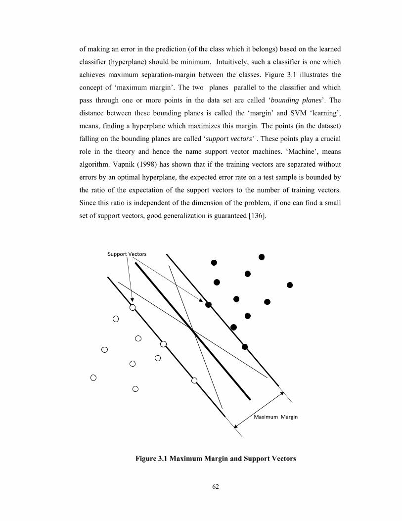
achieves maximum separation-margin between the classes. Figure 3.1 illustrates the
concept of ‘maximum margin’. The two planes parallel to the classifier and which
pass through one or more points in the data set are called ‘bounding planes’. The
distance between these bounding planes is called the ‘margin’ and SVM ‘learning’,
means, finding a hyperplane which maximizes this margin. The points (in the dataset)
falling on the bounding planes are called ‘support vectors’ . These points play a crucial
role in the theory and hence the name support vector machines. ‘Machine’, means
algorithm. Vapnik (1998) has shown that if the training vectors are separated without
errors by an optimal hyperplane, the expected error rate on a test sample is bounded by
the ratio of the expectation of the support vectors to the number of training vectors.
Since this ratio is independent of the dimension of the problem, if one can find a small
set of support vectors, good generalization is guaranteed [136].
Figure 3.1 Maximum Margin and Support Vectors
Maximum Margin
Support Vectors
63
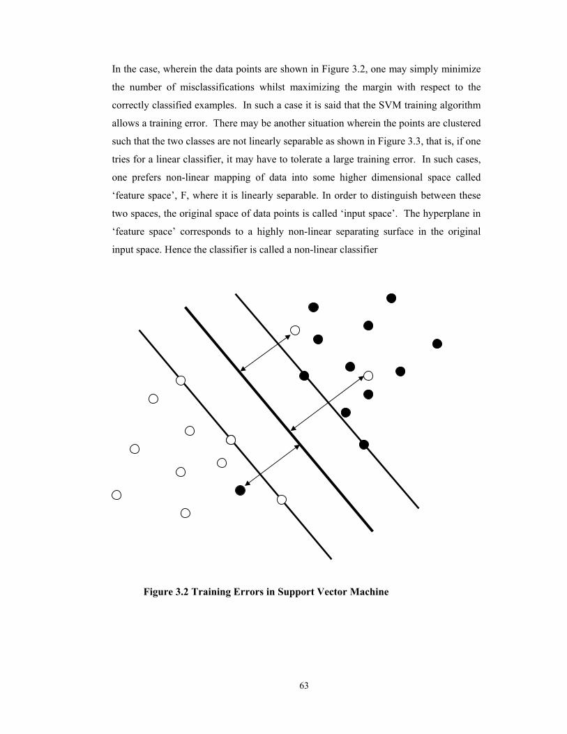
In the case, wherein the data points are shown in Figure 3.2, one may simply minimize
the number of misclassifications whilst maximizing the margin with respect to the
correctly classified examples. In such a case it is said that the SVM training algorithm
allows a training error. There may be another situation wherein the points are clustered
such that the two classes are not linearly separable as shown in Figure 3.3, that is, if one
tries for a linear classifier, it may have to tolerate a large training error. In such cases,
one prefers non-linear mapping of data into some higher dimensional space called
‘feature space’, F, where it is linearly separable. In order to distinguish between these
two spaces, the original space of data points is called ‘input space’. The hyperplane in
‘feature space’ corresponds to a highly non-linear separating surface in the original
input space. Hence the classifier is called a non-linear classifier
Figure 3.2 Training Errors in Support Vector Machine
64
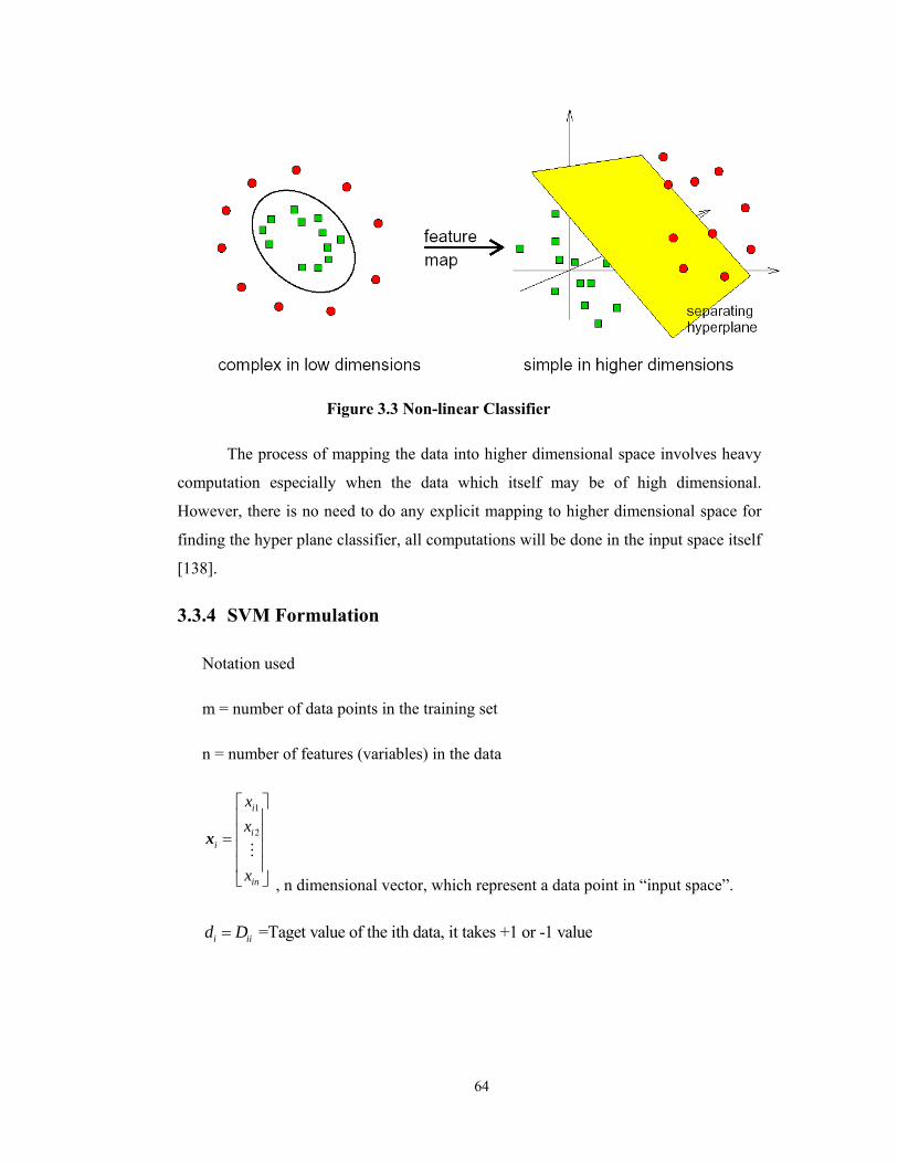
Figure 3.3 Non-linear Classifier
The process of mapping the data into higher dimensional space involves heavy
computation especially when the data which itself may be of high dimensional.
However, there is no need to do any explicit mapping to higher dimensional space for
finding the hyper plane classifier, all computations will be done in the input space itself
[138].
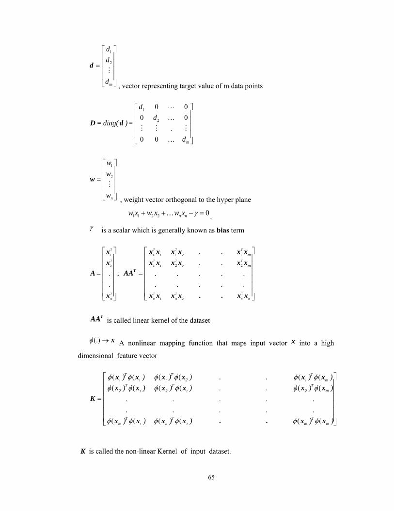
3.3.4 SVM Formulation
Notation used
m = number of data points in the training set
n = number of features (variables) in the data
1
2
i
ii
in
xx
x
⎡ ⎤⎢ ⎥⎢ ⎥=⎢ ⎥⎢ ⎥⎣ ⎦
x
, n dimensional vector, which represent a data point in “input space”.
=Taget value of the ith data, it takes +1 or -1 valuei iid D=
65
1
2
m
dd
d
⎡ ⎤⎢ ⎥⎢ ⎥=⎢ ⎥⎢ ⎥⎣ ⎦
d
, vector representing target value of m data points
1
2
0 00 0
.0 0 m
dd
diag( )=
d
⎡ ⎤⎢ ⎥⎢ ⎥⎢ ⎥⎢ ⎥⎣ ⎦
…
…
D = d
1
2
n
ww
w
⎡ ⎤⎢ ⎥⎢ ⎥=⎢ ⎥⎢ ⎥⎣ ⎦
w
, weight vector orthogonal to the hyper plane
1 1 2 2 0n nw x w x w x γ+ + − =… . γ is a scalar which is generally known as bias term
1 1 1 1
2 2 2 2
, .. . . .
T T T T
1 2
T T T T
1 2
T T T T
m m 1 m 2 m m
m
m
. .
. .. . . . .. .
⎡ ⎤ ⎡ ⎤⎢ ⎥ ⎢ ⎥⎢ ⎥ ⎢ ⎥⎢ ⎥ ⎢ ⎥= =⎢ ⎥ ⎢ ⎥⎢ ⎥ ⎢ ⎥⎢ ⎥ ⎢ ⎥⎣ ⎦ ⎣ ⎦
T
x x x x x x xx x x x x x x
A AA
x x x x x . . x x
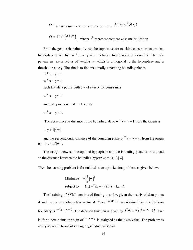
TAA is called linear kernel of the dataset
(.)φ → x A nonlinear mapping function that maps input vector x into a high
dimensional feature vector
( ( ( ( ( (( ( ( ( ( (
. . .( ( ( ( ( (
1 1 1 1
1 1
1 m 2
T T T2 m
T T T2 2 2 m
T T Tm m m
) ) ) ) . . ) )) ) ) ) . . ) ). . . . .. .
) ) ) ) ) )
φ φ φ φ φ φφ φ φ φ φ φ
φ φ φ φ φ φ
⎡ ⎤⎢ ⎥⎢ ⎥⎢ ⎥=⎢ ⎥⎢ ⎥⎢ ⎥⎣ ⎦
x x x x x xx x x x x x
K
x x x x . . x x
K is called the non-linear Kernel of input dataset.
66
Q = an mxm matrix whose (i,j)th element is ( ) ( )Ti j i jd d φ φx x
( ) K * T=Q . d * d, where *. represent element wise multiplication
From the geometric point of view, the support vector machine constructs an optimal
hyperplane given by w T x - γ = 0 between two classes of examples. The free
parameters are a vector of weights w which is orthogonal to the hyperplane and a
threshold value γ. The aim is to find maximally separating bounding planes
w T x - γ = 1
w T x - γ = -1
such that data points with d = -1 satisfy the constraints
w T x - γ ≤ -1
and data points with d = +1 satisfy
w T x - γ ≥ 1.
The perpendicular distance of the bounding plane w T x - γ = 1 from the origin is
|- γ + 1|/||w||
and the perpendicular distance of the bounding plane w T x - γ = -1 from the origin is, |- γ - 1|/||w|| .
The margin between the optimal hyperplane and the bounding plane is 1/||w||, and
so the distance between the bounding hyperplanes is 2/||w||.
Then the learning problem is formulated as an optimization problem as given below.
The ‘training of SVM’ consists of finding w and γ, given the matrix of data points
A and the corresponding class vector d. Once and γw are obtained then the decision
boundary is 0− γ =Tw x . The decision function is given by ( )f x = sign( )− γTw x . That
is, for a new points the sign of − γTw x is assigned as the class value. The problem is
easily solved in terms of its Lagrangian dual variables.
.,,1,1)( subject to21 Minimize 2
liD iT
ii …=≥−
=
γxw
w
67
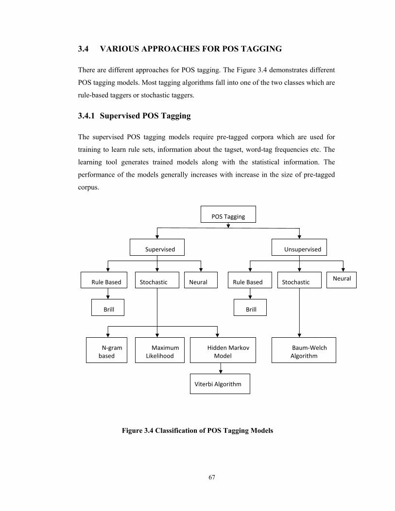
3.4 VARIOUS APPROACHES FOR POS TAGGING
There are different approaches for POS tagging. The Figure 3.4 demonstrates different
POS tagging models. Most tagging algorithms fall into one of the two classes which are
rule-based taggers or stochastic taggers.
3.4.1 Supervised POS Tagging
The supervised POS tagging models require pre-tagged corpora which are used for
training to learn rule sets, information about the tagset, word-tag frequencies etc. The
learning tool generates trained models along with the statistical information. The
performance of the models generally increases with increase in the size of pre-tagged
corpus.
Figure 3.4 Classification of POS Tagging Models
POS Tagging
UnsupervisedSupervised
Rule Based Stochastic Neural Rule Based Stochastic Neural
Brill Brill
N‐gram based
Maximum Likelihood
Hidden Markov Model
Baum‐Welch Algorithm
Viterbi Algorithm
68
3.4.2 Unsupervised POS Tagging
Unlike the supervised models, the unsupervised POS tagging models do not require a
pre-tagged corpus. Instead, they use advanced computational methods like the Baum-
Welch algorithm to automatically induce tagsets, transformation rules etc. Based on the
information, they either calculate the probabilistic information needed by the stochastic
taggers or induce the contextual rules needed by rule-based systems or transformation
based systems.
3.4.3 Rule based POS Tagging
The rule based POS tagging models apply a set of hand written rules and use contextual
information to assign POS tags to words in a sentence. These rules are often known as
context frame rules. For example, a context frame rule might say something like:
“If an ambiguous/unknown word X is preceded by a Determiner and followed by a
Noun, tag it as an Adjective.”
On the other hand, the transformation based approaches use a pre-defined set of
handcrafted rules as well as automatically induced rules that are generated during
training. Some models also use information about capitalization and punctuation, the
usefulness of which are largely dependent on the language being tagged. The earliest
algorithms for automatically assigning Part-of-Speech were based on two-stage
architecture. The first stage used a dictionary to assign each word a list of potential
parts of speech. The second stage used large lists of hand-written disambiguation rules
to bring down this list to a single Part-of-Speech for each word [139].
The ENGTWOL [140] tagger is based on the same two-stage architecture,
although both the lexicon and the disambiguation rules are much more sophisticated
than the early algorithms. The ENGTWOL lexicon is based on the two-level
morphology. It has about 56,000 entries for English word stems, counting a word with
multiple parts of speech (e.g. nominal and verbal senses of hit) as separate entries, and
of course not counting inflected and many derived forms. Each entry is annotated with
a set of morphological and syntactic features. In the first stage of the tagger, each word
is run through the two-level lexicon transducer and the entries for all possible parts of
speech are returned.
69
3.4.4 Stochastic POS Tagging
A stochastic approach includes frequency, probability or statistics. The simplest
stochastic approach finds out the most frequently used tag for a specific word in the
annotated training data and uses this information to tag that word in the unannotated
text. The problem with this approach is that it can come up with sequences of tags for
sentences that are not acceptable according to the grammar rules of a language.
An alternative to the word frequency approach is known as the n-gram approach
that calculates the probability of a given sequence of tags. It determines the best tag for
a word by calculating the probability that it occurs with the n previous tags, where the
value of n is set to 1, 2 or 3 for practical purposes. These are known as the unigram,
bigram and trigram models. The most common algorithm for implementing an n-gram
approach for tagging a new text is known as the Viterbi Algorithm, which is a search
algorithm that avoids the polynomial expansion of a breadth first search by trimming
the search tree at each level using the best m Maximum Likelihood Estimates (MLE)
where m represents the number of tags of the following word.
Advantages of Statistical Approach,
• Very robust, can process any input strings
• Training is automatic, very fast
• Can be retrained for different corpora / tagsets without much effort
• Language independent
• Minimize the human effort and human error.
3.4.5 Other Techniques
Apart from these, a few different approaches for tagging have been developed.
Support Vector Machines: This is the powerful machine learning method used for
various applications in NLP and other areas like bio-informatics, data mining, etc.
Neural Networks: These are potential candidates for the classification task since
they learn abstractions from examples [141].
70
Decision Trees: These are classification devices based on hierarchical clusters of
questions. They have been used for natural language processing such as POS Tagging.
“Weka” can be used for classifying the ambiguous words [141].
Maximum Entropy Models: These avoid certain problems of statistical
interdependence and have proven successful for tasks such as parsing and POS tagging.
Example-Based Techniques: These techniques find the training instance that is
most similar to the current problem instance and assume the same class for the new
problem instance as for the similar one.
3.5 VARIOUS APPROACHES FOR MORPHOLOGICAL
ANALYZER
3.5.1 Two level Morphological Analysis
Koskenniemi (1985) [26] describes two-level morphology as a “general, language
independent framework which has been implemented for a host of different languages
(Finnish, English, Russian, Swedish, German, Swahili, Danish, Basque, Estonian,
etc.)”. It consists of two representations and one relation.
The surface representation of a word-form:
This is the actual spelling of the final valid word. For example English words
eating and swimming, are both surface representations.
The lexical (also called morphophonemic) representation of a word-form:
This shows a simple concatenation of base forms and tags. Consider the
following examples showing the lexical and surface form of English words.
Lexical Form Surface Form
talk + Verb talk
walk + Verb + 3PSg walks
eat +Verb + Prog eating
swim +Verb + Prog swimming
71
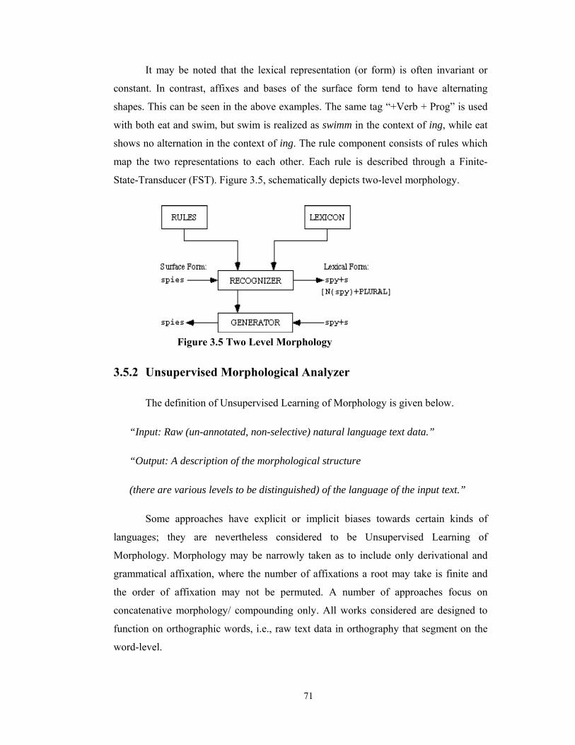
It may be noted that the lexical representation (or form) is often invariant or
constant. In contrast, affixes and bases of the surface form tend to have alternating
shapes. This can be seen in the above examples. The same tag “+Verb + Prog” is used
with both eat and swim, but swim is realized as swimm in the context of ing, while eat
shows no alternation in the context of ing. The rule component consists of rules which
map the two representations to each other. Each rule is described through a Finite-
State-Transducer (FST). Figure 3.5, schematically depicts two-level morphology.
Figure 3.5 Two Level Morphology
3.5.2 Unsupervised Morphological Analyzer
The definition of Unsupervised Learning of Morphology is given below.
“Input: Raw (un-annotated, non-selective) natural language text data.”
“Output: A description of the morphological structure
(there are various levels to be distinguished) of the language of the input text.”
Some approaches have explicit or implicit biases towards certain kinds of
languages; they are nevertheless considered to be Unsupervised Learning of
Morphology. Morphology may be narrowly taken as to include only derivational and
grammatical affixation, where the number of affixations a root may take is finite and
the order of affixation may not be permuted. A number of approaches focus on
concatenative morphology/ compounding only. All works considered are designed to
function on orthographic words, i.e., raw text data in orthography that segment on the
word-level.
72
3.5.3 Memory based Morphological Analysis
Memory based learning approach models morphological analysis (including
compounding) of complex word-forms as sequences of classification tasks. MBMA
(Memory-Based Morphological Analysis) is a memory-based learning system (Stanfill
and Waltz, 1986) [142]. Memory-based learning is a class of inductive, supervised
machine learning algorithm that learns by storing examples of a task in memory.
Computational effort is invested on a "call-by-need" basis for solving new examples
(henceforth called instances) of the same task. When new instances are presented to a
memory-based learner, it searches for the best matching instances in memory,
according to a task-dependent similarity metric. When it has found the best matches
(the nearest neighbors), it transfers their solution (classification, label) to the new
instance.
3.5.4 Stemmer based Approach
Stemmer uses a set of rules containing list of stems and replacement rules to stripping
of affixes. It is a program oriented approach where the developer has to specify all
possible affixes with replacement rules. Potter algorithm is one of the most widely used
stemmer algorithm and it is freely available. The advantage of stemmer algorithm is
that it is very suitable to highly agglutinative languages like Dravidian languages for
creating Morphological Analyzer and Generator.
3.5.5 Suffix Stripping based Approach
Highly agglutinative languages such as Dravidian languages, a Morphological Analyzer
and Generator can be successfully built using suffix stripping approach. The advantage
of the Dravidian language is that no prefixes and circumfixes exist for words. Words
are usually formed by adding suffixes to the root word serially. This property can be
well suited for suffix stripping based Morphological Analyzer and Generator. Once the
suffix is identified, the stem of the whole word can be obtained by removing that suffix
and applying proper orthographic (sandhi) rules. A set of dictionaries like stem
dictionary, suffix dictionary and also using morphotactics and sandhi rules, a suffix
stripping algorithm successfully implements MAG.
73
3.6 VARIOUS APPROACHES IN MACHINE TRANSLATION
From the period when the first idea of using machine for the process of language
translation, there have been many different approaches to machine translation that have
been proposed, implemented and put into use, during the course of time. The main
approaches to machine translation are:
• Linguistic or Rule Based Approaches
o Direct Approach
o Interlingua Approach
o Transfer Approach
• Non-Linguistic Approaches
o Dictionary Based Approach
o Corpus Based Approach
o Example Based Approach
o Statistical Approach
• Hybrid Approach
Direct, Interlingua and Transfer approaches are linguistic approaches which require
some sort of linguistic knowledge to perform translations, whereas dictionary based,
example based and statistical approach falls under non-linguistic approaches that don’t
require any linguistic knowledge to translate the sentences. Hybrid approach is a
combination of both linguistic and non-linguistic approaches.
3.6.1 Linguistic or Rule Based Approaches
Rule based approaches requires a lot of linguistic knowledge during the translation and
so it uses grammar rules and computer programs which will be helpful in analysing the
text for determining grammatical information and features for each and every word in
the source language, translating it by replacing each word by lexicon or word that have
the same context in the target language. Rule based approach is the principal
methodology that was developed in machine translation. Linguistic knowledge will be
required in order to write the rules for this type of approaches. These rules will play a
vital role during the different levels of translation. This approach is also called as
Theory based Machine Translation.
74
The benefit of rule based machine translation method is that it can intensely
examine the sentence at its syntax and semantic levels. There are complications in this
method such as prerequisite of vast linguistic knowledge and very huge number of rules
is needed in order to cover all the features in a language. An advantage of the approach
is that the developer has more control over the translations than is the case with corpus-
based approaches. The three different approaches that require linguistic knowledge are
as follows.
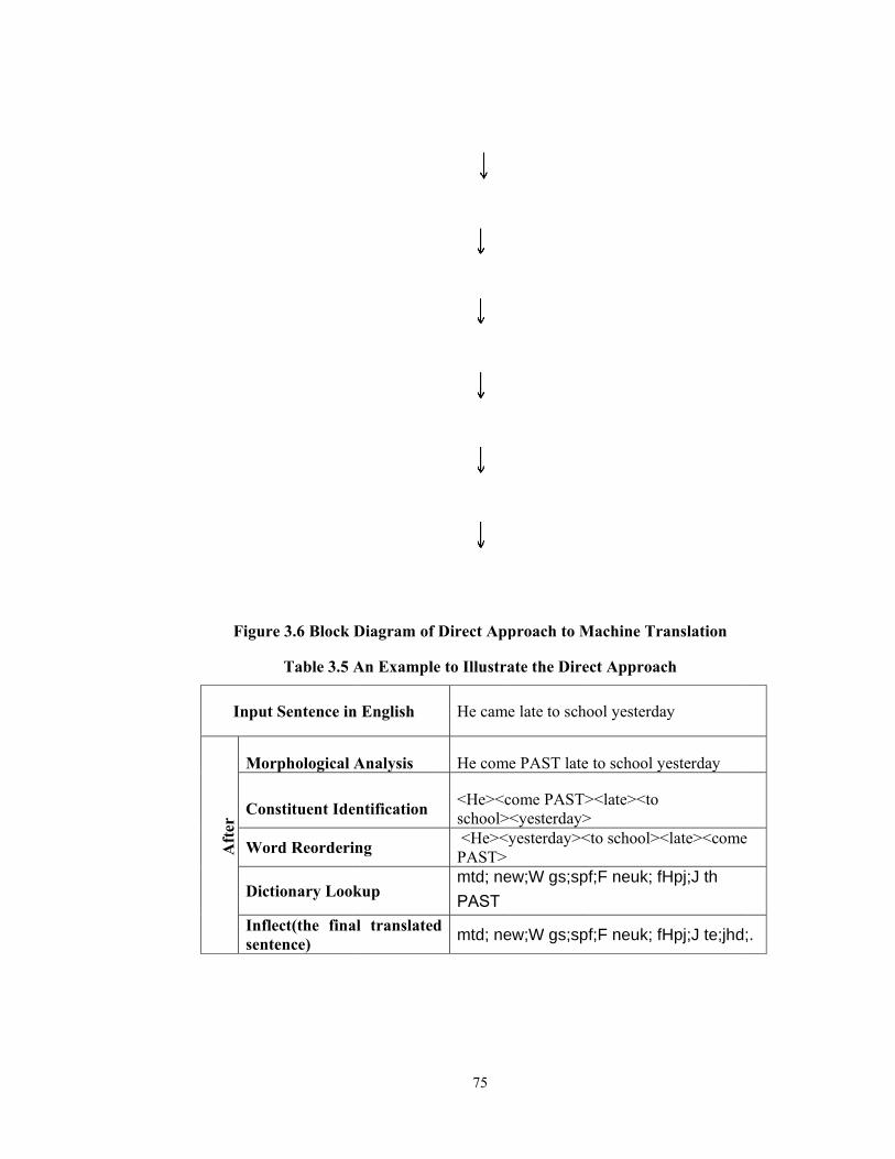
3.6.1.1 Direct Approach
Direct translation approach can be considered as the first approach to machine
translation. In this type of approach, the machine translation system is designed more
specifically for one particular pair of language. There is no need of identifying the
schematic roles and universal concepts in this approach. It involves the process of
analysing morphological information, identify the constituents and reorder the words in
the source language according to the word order pattern of the target language and then
replace the words in the source language by the target language words using a lexical
dictionary of that particular language pair and as a last step, inflect the words
appropriately to produce translations. This approach as it is seen, looks like a lot of
work has to be done in order to produce translations, but all those work which has to be
employed will be simple and can be accomplished very easily, in a short span of time.
Figure 3.5 illustrates the block diagram of the direct approach to machine translation.
This approach perform a simple and minimal syntactic and semantic analysis,
by which it differs from the other rule based translation systems such as interlingua and
the transfer-based approaches. As the direct approach to machine translation is
considered to be ad-hoc and found to be an approach that is unsuitable approach to
machine translation. Table 3.6 describes the example, how the sentence “he came late
to school yesterday” will be translated from English to Tamil using the direct approach.
Figure
Input
Aft
er
Mor
Con
Wor
Dict
Inflesent
e 3.6 Block
Table 3.5 A
Sentence in
rphological
nstituent Ide
rd Reorderi
tionary Loo
ect(the finaence)
Diagram of
An Exampl
n English
Analysis
entification
ing
kup
al translate
75
f Direct App
le to Illustra
He came
He come
<He><cschool>< <He><yPAST>mtd; nePAST
ed mtd; ne
proach to M
ate the Dire
e late to scho
e PAST late
come PAST><yesterday>yesterday><
ew;W gs;spf
ew;W gs;spf
Machine Tra
ct Approac
ool yesterday
to school ye
><late><to > <to school><
f;F neuk; fH
f;F neuk; fH
anslation
h
y
esterday
<late><come
Hpj;J th
Hpj;J te;jhd;
e
;.
76
3.6.1.2 Interlingua Approach
Interlingua approach to machine translation mainly aims at transforming the texts in the
source language to a common representation which is applicable to many languages.
Using this representation the translation of text to the target language is performed and
it should be possible to translate to every language from the same Interlingua
representation with the right rules.
Interlingua approach sees machine translation as a two stage process:
1. Analysing and transforming the source language texts into a common language
independent representation.
2. From the common language independent form generate the text in the target
language.
The first stage is particular to source language and doesn’t require any knowledge
about the target language whereas the second stage is particular to the target language
and doesn’t require any knowledge from the source language. The main advantage of
interlingua approach is that it creates an economical multilingual environment that
requires 2n translation systems to translate among n languages where in the other case,
the direct approach requires n(n-1) translation systems. Table 3.6 has the Interlingua
representation of the sentence, “he will reach the hospital in ambulance”.
Table 3.6 An Example for Interlingua Representation
Predicate Reach
Agent Boy (Number: Singular)
Theme Hospital (Number: Singular)
Instrument Ambulance (Number: Singular)
Tense FUTURE
The concepts and relations that are used are the most important aspect in any
interlingua-based system. The ontology should be powerful enough that all subtleties of
meaning that can be expressed using any language should be representable in the
Interlingua. Interlingua approach can be found more economical when translation is
car
inc
sho
3.6
Th
rep
Int
syn
or
gen
sen
sta
stru
exp
blo
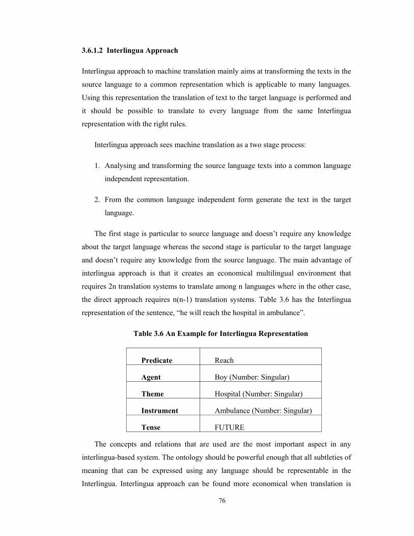
rried out wit
creased, dram
own in the F
6.1.3 Transf
e less deter
presentations
erlingua app
ntactic or sem
semantic dep
The transf
neration. In
ntence struct
ge, transfor
ucture to tha
presses the t
ock diagram
th three or m
matically. T
igure 3.7.
fer Approac
rmined trans
s of the sour
proach. The
mantic infor
pending on t
fer model
the analysi
ture and the
mations are
at of the targ
tense, numb
of the transf
more languag
This is clearl
Figure 3.7
ch
sfer approac
rce and targe
e transfer ap
rmation of th
the need.
involves th
is stage, the
e constituent
e applied to
get language
ber, gender e
fer approach
77
ges but also
ly evident f
7 The Vauqu
ch has three
et language t
pproach can
he text. In ge
hree stages
e source lan
ts of the sen
the source
e. The gene
etc. in the ta
h.
the complex
from the Va
uois Triangl
e stages, co
texts, instead
n be done e
eneral, transf
which are
nguage sent
ntence are i
language p
ration stage
arget langua
xity of this a
auquois trian
le
omprising th
d of the two
either by co
fer can eithe
analysis,
tence is par
identified. In
parse tree to
translates th
age. Figure 3
approach ge
ngle which
he intellectu
o stages in th
onsidering th
er be syntact
transfer, an
rsed, and th
n the transfe
o convert th
he words an
3.8 shows th
ets
is
ual
he
he
tic
nd
he
fer
he
nd
he
thr
rep
sta
ord
fin
wo
pro
gen
sen
tran
sin
lan
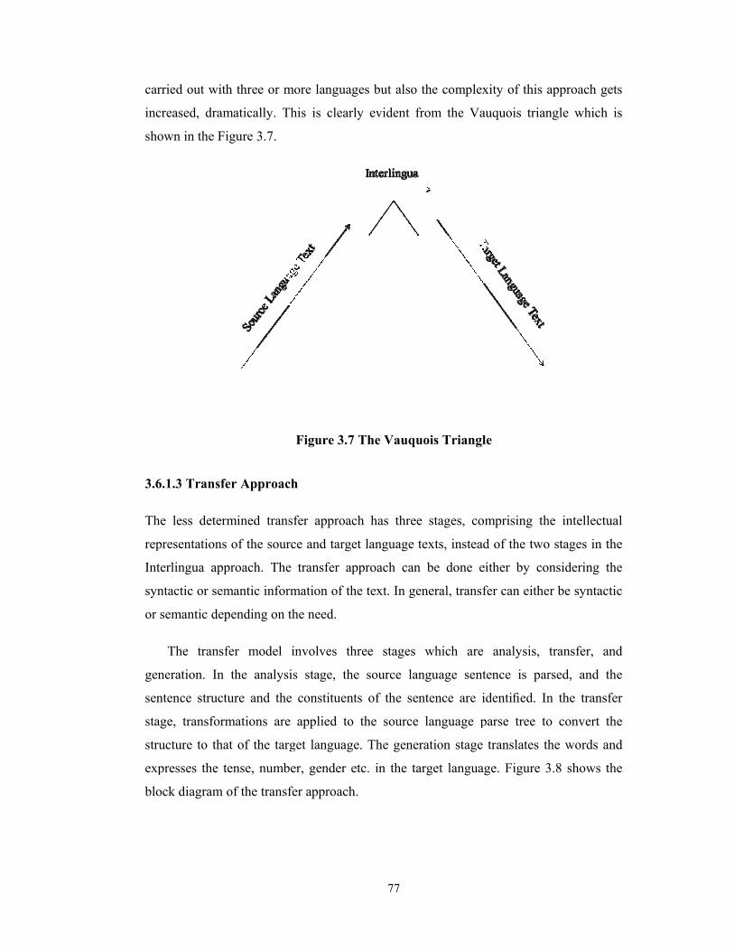
Consider t
ee stages of
presentation
ge. The repr
der as result
al generatio
ords.
From the a
oduces a rep
nerates the f
ntence. Thus
nslate n lang
nce individua
nguages for e
Figure
the sentence
f the translati
after the an
resentation o
of the trans
on stage wh
above examp
presentation
final translat
s, using thi
guages, will
al transfer c
each directio
3.8 Block D
e, “he will c
ion of this se
nalysis stage
of the senten
fer stage of
ich replaces
ple, it will b
that is sour
tion from the
is approach
require ‘n’ a
components
on and ‘n’ ge
78
Diagram for
come to scho
entence usin
e of the tran
ce after reor
the transfer
s the source
be clear that
rce language
e target lang
in multilin
analyser com
are require
eneration com
r Transfer A
ool in bus”.
ng the transfe
nsfer approa
rdering it acc
approach is
e language w
t, the analys
e dependent
guage depend
ngual machin
mponents, n(
ed for transl
mponents.
Approach
Table 3.7
er approach.
ach is show
cording to th
s shown in T
words to tar
ser stage of
and the gen
dent represe
ne translatio
(n-1) transfe
lation betwe
illustrates th
The sentenc
wn in analys
he Tamil wor
Table 3.7. Th
rget languag
this approac
neration stag
entation of th
on system t
er componen
een a pair o
he
ce
sis
rd
he
ge
ch
ge
he
to
nts
of
79
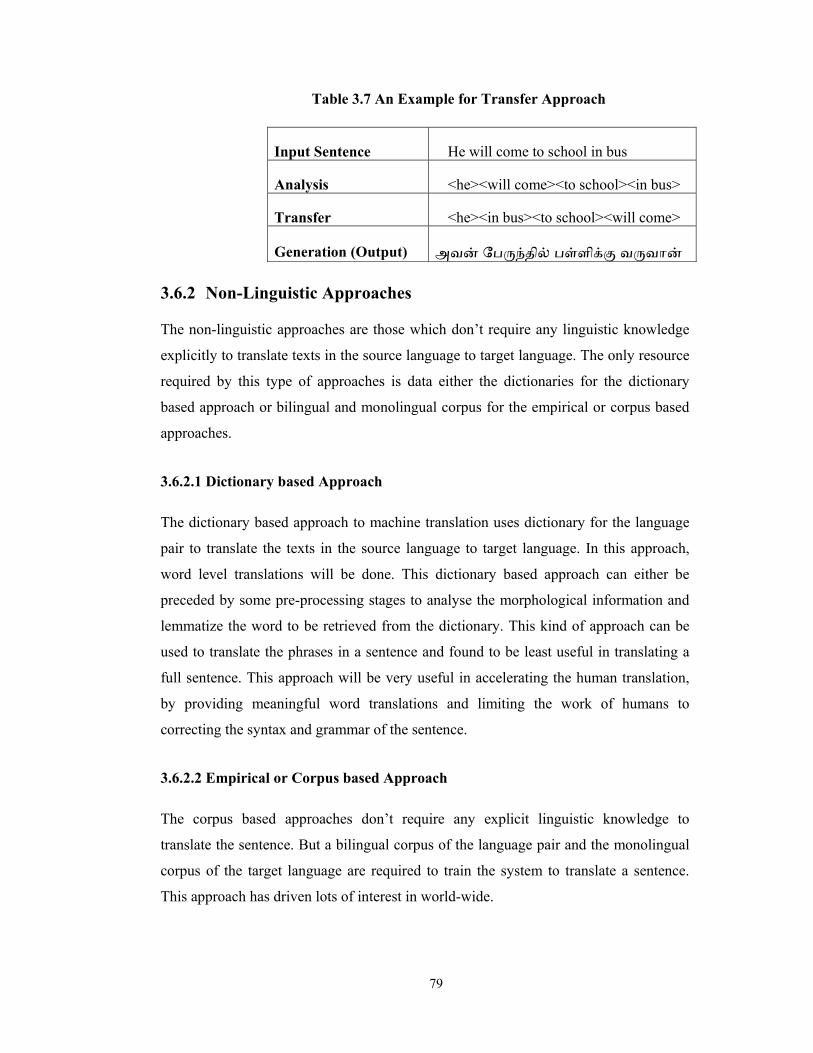
Table 3.7 An Example for Transfer Approach
Input Sentence He will come to school in bus
Analysis <he><will come><to school><in bus>
Transfer <he><in bus><to school><will come>
Generation (Output) அவன் ேப ந்தில் பள்ளிக்கு வ வான்
3.6.2 Non-Linguistic Approaches
The non-linguistic approaches are those which don’t require any linguistic knowledge
explicitly to translate texts in the source language to target language. The only resource
required by this type of approaches is data either the dictionaries for the dictionary
based approach or bilingual and monolingual corpus for the empirical or corpus based
approaches.
3.6.2.1 Dictionary based Approach
The dictionary based approach to machine translation uses dictionary for the language
pair to translate the texts in the source language to target language. In this approach,
word level translations will be done. This dictionary based approach can either be
preceded by some pre-processing stages to analyse the morphological information and
lemmatize the word to be retrieved from the dictionary. This kind of approach can be
used to translate the phrases in a sentence and found to be least useful in translating a
full sentence. This approach will be very useful in accelerating the human translation,
by providing meaningful word translations and limiting the work of humans to
correcting the syntax and grammar of the sentence.
3.6.2.2 Empirical or Corpus based Approach
The corpus based approaches don’t require any explicit linguistic knowledge to
translate the sentence. But a bilingual corpus of the language pair and the monolingual
corpus of the target language are required to train the system to translate a sentence.
This approach has driven lots of interest in world-wide.
3.6
Th
bei
into
typ
Th
tran
is a
sen
retu
rep
alig
pre
the
ma
or
targ
usi
Fin
usi
exa
6.2.3 Examp
is approach
ings interpre
o sub proble
pe of similar
is approach
nslation has
The EB
a computer
ntence or a s
urned. In co
produce prev
gnment, and
evious exam
e input sente
atch to match
identify gen
get words th
ing existing
nally, these
ing either he
ample-based
ple based Ap
to machine
et and solve t
ems, solve ea
r problems in
h needs a h
to be perfor
BMT system
aided transl
imilar senten
ontrast, the
vious senten
d recombinat
mples and fin
nce. This m
hes using hig
neralized tem
hese matchin
bilingual dic
corresponde
euristic or st
d approach.
Figu
pproach
translation i
the problem
ach of the su
n the past an
huge bilingu
rmed.
m functions l
lation tool t
nce has been
EBMT sys
nce translati
tion [143]. 1
nds the piece
matching is do
gher linguist
mplates. 2) T
ng strings co
ctionaries or
ences are rec
tatistical info
ure 3.9 Bloc
80
s a techniqu
ms. That is, n
ub problems
nd integrate
ual corpus o
like a transla
that is able
n translated p
tem can tra
ons. EBMT
) In matchin
es of text th
one using va
tic knowledg
The alignmen
orrespond to
r automatica
combined an
ormation. Fi
ck Diagram
ue that is mai
ormally the
with the ide
them to sol
of the lang
ation memor
to reuse pre
previously, t
anslate nove
T translates i
ng, the system
at together g
arious heuris
ge to calcula
nt step is the
o. This ident
ally deduced
nd the rejoin
igure 3.9 sho
of EBMT S
inly based o
humans spli
ea of how th
lve the probl
guage pair a
ry. A transla
evious transl
the previous
el sentences
in three step
m looks in i
give the bes
stics from ex
ate the simila
en used to id
tification ca
from the pa
ned sentenc
ows the bloc
System
n how huma
it the problem
ey solved th
lem in whol
among whic
ation memor
lations. If th
s translation
and not ju
ps; matchin
ts database o
st coverage o
xact characte
arity of word
dentify whic
an be done b
arallel data. 3
es are judge
ck diagram o
an
m
his
le.
ch
ry
he
is
ust
g,
of
of
er
ds
ch
by
3)
ed
of
bou
sen
the
sec
of
pro
not
3.6
Sta
me
cor
ma
Tra
In orde
ught a home
The pa
ntences in th
e words in th
cond sentenc
the sentence
ocessing may
t available in
6.2.4 Statisti
atistical app
ethods by d
rpora. This
any aspects.
anslation (SM
r to get a cle
e” and the Ta
Tab
arts of the s
he corpus. H
he first sent
ce pair. Ther
es in the cor
y be require
n the corpus.
ical Approa
proach to m
deriving the
approach di
Figure 3.10
MT) system.
Figu
ear idea of t
amil translat
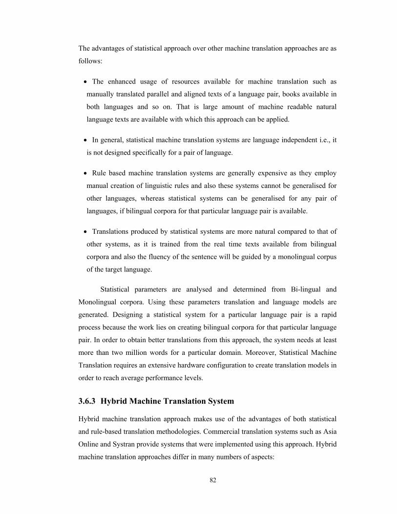
ble 3.8 Exam
EnglishHe bought a
He has a ho
sentence to
Here, the par
tence pair an
refore, the co
rpus are take
ed in order t
.
ach
machine tran
parameters
iffers from
0 shows the
.
ure 3.10 Blo
81
this approach
tion also giv
mple of Eng
h a pen
ome
be translate
rt of the sent
nd ‘a home’
orresponding
en and comb
o handle nu
nslation gen
for those
the other ap
e simple blo
ock Diagram
h, consider t
en in Table
glish and Ta
mtd; xmtDf;F
ed will be
tence ‘He bo
gets match
g Tamil part
bined approp
umbers and g
nerates tran
methods by
pproaches t
ock diagram
m of SMT S
the English
3.8.
amil Senten
TamilU ngdh thF xU tPL ,
matched wi
ought’ gets
hed with the
t of the matc
priately. Som
gender if ex
nslations usi
y analysing
to machine
of a Statist
System
sentence “H
nces
l h';fpdhd; Uf;fpwJ
ith these tw
matched wit
words in th
ched segmen
metimes, pos
act words ar
ing statistic
the bilingu
translation i
tical Machin
He
wo
th
he
nts
st-
re
al
ual
in
ne
82
The advantages of statistical approach over other machine translation approaches are as
follows:
• The enhanced usage of resources available for machine translation such as
manually translated parallel and aligned texts of a language pair, books available in
both languages and so on. That is large amount of machine readable natural
language texts are available with which this approach can be applied.
• In general, statistical machine translation systems are language independent i.e., it
is not designed specifically for a pair of language.
• Rule based machine translation systems are generally expensive as they employ
manual creation of linguistic rules and also these systems cannot be generalised for
other languages, whereas statistical systems can be generalised for any pair of
languages, if bilingual corpora for that particular language pair is available.
• Translations produced by statistical systems are more natural compared to that of
other systems, as it is trained from the real time texts available from bilingual
corpora and also the fluency of the sentence will be guided by a monolingual corpus
of the target language.
Statistical parameters are analysed and determined from Bi-lingual and
Monolingual corpora. Using these parameters translation and language models are
generated. Designing a statistical system for a particular language pair is a rapid
process because the work lies on creating bilingual corpora for that particular language
pair. In order to obtain better translations from this approach, the system needs at least
more than two million words for a particular domain. Moreover, Statistical Machine
Translation requires an extensive hardware configuration to create translation models in
order to reach average performance levels.
3.6.3 Hybrid Machine Translation System
Hybrid machine translation approach makes use of the advantages of both statistical
and rule-based translation methodologies. Commercial translation systems such as Asia
Online and Systran provide systems that were implemented using this approach. Hybrid
machine translation approaches differ in many numbers of aspects:
Ru
ma
targ
stat
for
Sta
app
sys
the
sys
sho
3.7
Th
sys
two
aut
sho
aut
flu
pro
ule-based sys
achine transl
get languag
tistical syste
r this system
Fig
atistical tran
proach a sta
stem to pre-p
e output of
stem to prov
own in Figur
Figure
7 EVAL
is section p
stem. Evalua
o important
tomatic eval
ows how to
tomatically.
ency is thro
ocess. The j
stem with p
ation system
e. The outp
em to provid
.
gure 3.11 Ru
nslation syst
atistical mac
process the
the statistic
vide better
re 3.12.
3.12 Statist
LUATING
provides eva
ation of mac
t types of
luation and
o evaluate
The most
ough human
udgments o
post-processi
m produces t
put of this r
de better tra
ule based Tr
tem with pre
chine transla
data before
al system c
translations.
tical Machin
G STATIST
aluation met
chine transla
evaluation
manual eva
the perform
reliable me
evaluation.
of more than
83
ing by statis
translations f
rule based
anslations. F
ranslation S
e-processing
ation system
providing th
can also be
. The block
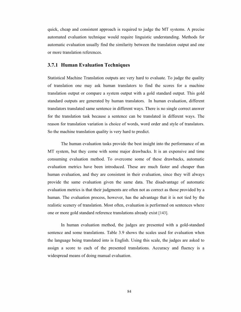
ne Translat
TICAL M
thods to find
ation is a ve
techniques
aluation or
mance of an
ethod for e
But human
n one huma
stical appro
for a given t
system will
Figure 3.11 s
System with
g by the rule
m is incorpo
he data for t
post-process
k diagram fo
tion System
MACHINE
d the qualit
ry active fie
in machin
human eval
n MT syst
evaluating tr
n evaluation
an evaluator
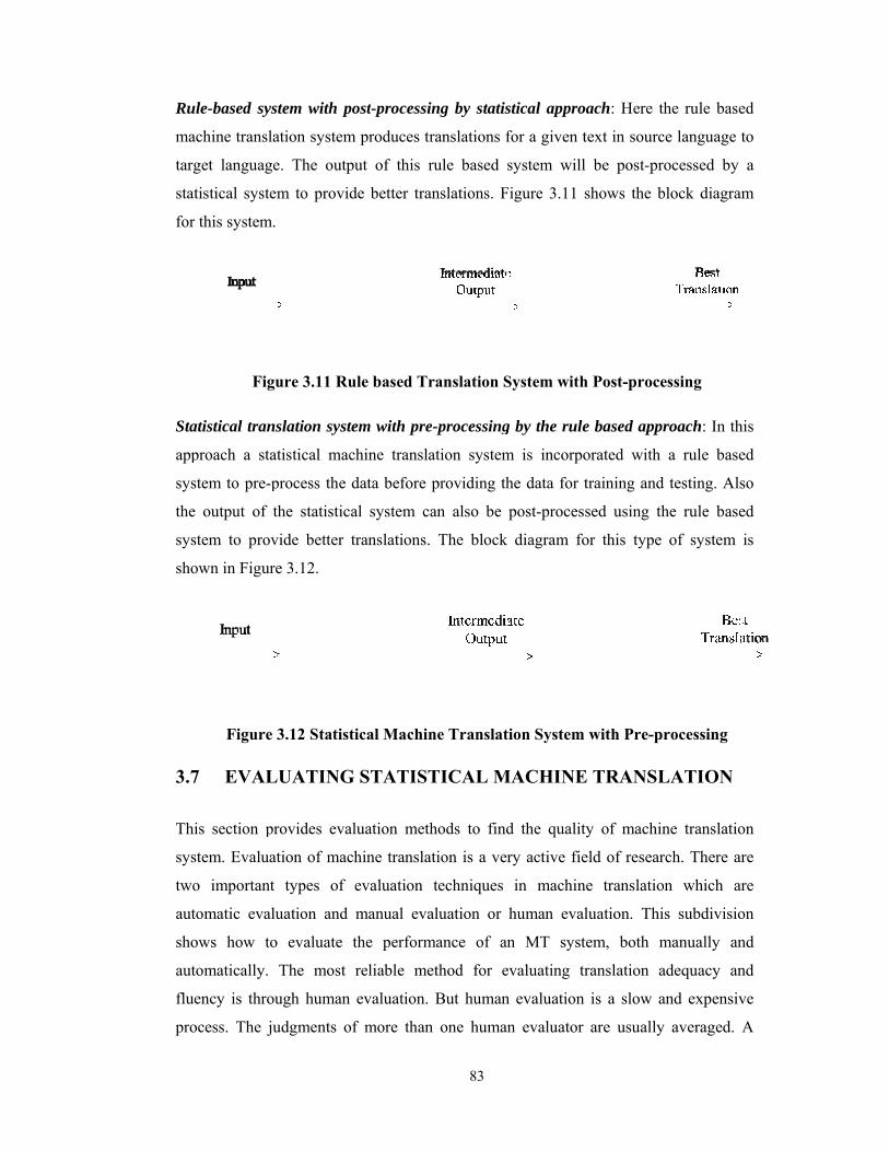
oach: Here th
text in sourc
l be post-pr
shows the b
h Post-proce
e based appr
orated with
training and
sed using th
or this type
with Pre-p
E TRANSL
ty of machin
eld of resear
ne translatio
luation. Thi
tem, both m
ranslation a
is a slow a
are usually
he rule base
ce language t
ocessed by
block diagram
essing
roach: In th
a rule base
d testing. Als
he rule base
of system
rocessing
LATION
ne translatio
rch. There ar
on which ar
is subdivisio
manually an
adequacy an
and expensiv
y averaged.
ed
to
a
m
his
ed
so
ed
is
on
re
re
on
nd
nd
ve
A
84
quick, cheap and consistent approach is required to judge the MT systems. A precise
automated evaluation technique would require linguistic understanding. Methods for
automatic evaluation usually find the similarity between the translation output and one
or more translation references.
3.7.1 Human Evaluation Techniques
Statistical Machine Translation outputs are very hard to evaluate. To judge the quality
of translation one may ask human translators to find the scores for a machine
translation output or compare a system output with a gold standard output. This gold
standard outputs are generated by human translators. In human evaluation, different
translators translated same sentence in different ways. There is no single correct answer
for the translation task because a sentence can be translated in different ways. The
reason for translation variation is choice of words, word order and style of translators.
So the machine translation quality is very hard to predict.
The human evaluation tasks provide the best insight into the performance of an
MT system, but they come with some major drawbacks. It is an expensive and time
consuming evaluation method. To overcome some of these drawbacks, automatic
evaluation metrics have been introduced. These are much faster and cheaper than
human evaluation, and they are consistent in their evaluation, since they will always
provide the same evaluation given the same data. The disadvantage of automatic
evaluation metrics is that their judgments are often not as correct as those provided by a
human. The evaluation process, however, has the advantage that it is not tied by the
realistic scenery of translation. Most often, evaluation is performed on sentences where
one or more gold standard reference translations already exist [143].
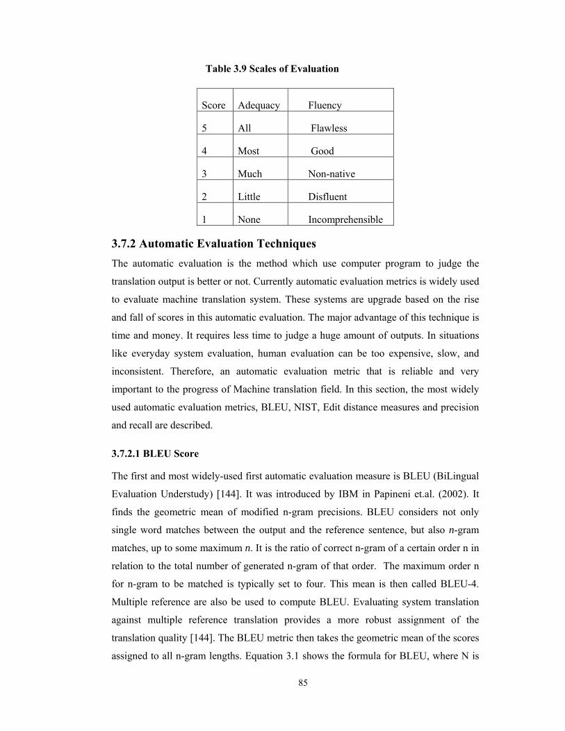
In human evaluation method, the judges are presented with a gold-standard
sentence and some translations. Table 3.9 shows the scales used for evaluation when
the language being translated into is English. Using this scale, the judges are asked to
assign a score to each of the presented translations. Accuracy and fluency is a
widespread means of doing manual evaluation.
85
Table 3.9 Scales of Evaluation
Score Adequacy Fluency
5 All Flawless
4 Most Good
3 Much Non-native
2 Little Disfluent
1 None Incomprehensible
3.7.2 Automatic Evaluation Techniques The automatic evaluation is the method which use computer program to judge the
translation output is better or not. Currently automatic evaluation metrics is widely used
to evaluate machine translation system. These systems are upgrade based on the rise
and fall of scores in this automatic evaluation. The major advantage of this technique is
time and money. It requires less time to judge a huge amount of outputs. In situations
like everyday system evaluation, human evaluation can be too expensive, slow, and
inconsistent. Therefore, an automatic evaluation metric that is reliable and very
important to the progress of Machine translation field. In this section, the most widely
used automatic evaluation metrics, BLEU, NIST, Edit distance measures and precision
and recall are described.
3.7.2.1 BLEU Score
The first and most widely-used first automatic evaluation measure is BLEU (BiLingual
Evaluation Understudy) [144]. It was introduced by IBM in Papineni et.al. (2002). It
finds the geometric mean of modified n-gram precisions. BLEU considers not only
single word matches between the output and the reference sentence, but also n-gram
matches, up to some maximum n. It is the ratio of correct n-gram of a certain order n in
relation to the total number of generated n-gram of that order. The maximum order n
for n-gram to be matched is typically set to four. This mean is then called BLEU-4.
Multiple reference are also be used to compute BLEU. Evaluating system translation
against multiple reference translation provides a more robust assignment of the
translation quality [144]. The BLEU metric then takes the geometric mean of the scores
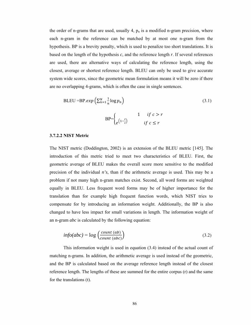
assigned to all n-gram lengths. Equation 3.1 shows the formula for BLEU, where N is
86
the order of n-grams that are used, usually 4, pn is a modified n-gram precision, where
each n-gram in the reference can be matched by at most one n-gram from the
hypothesis. BP is a brevity penalty, which is used to penalize too short translations. It is
based on the length of the hypothesis c, and the reference length r. If several references
are used, there are alternative ways of calculating the reference length, using the
closest, average or shortest reference length. BLEU can only be used to give accurate
system wide scores, since the geometric mean formulation means it will be zero if there
are no overlapping 4-grams, which is often the case in single sentences.
BLEU =BP. ∑ log (3.1)
BP=1
3.7.2.2 NIST Metric
The NIST metric (Doddington, 2002) is an extension of the BLEU metric [145]. The
introduction of this metric tried to meet two characteristics of BLEU. First, the
geometric average of BLEU makes the overall score more sensitive to the modified
precision of the individual n’s, than if the arithmetic average is used. This may be a
problem if not many high n-gram matches exist. Second, all word forms are weighted
equally in BLEU. Less frequent word forms may be of higher importance for the
translation than for example high frequent function words, which NIST tries to
compensate for by introducing an information weight. Additionally, the BP is also
changed to have less impact for small variations in length. The information weight of
an n-gram abc is calculated by the following equation:
info(abc) = log
(3.2)
This information weight is used in equation (3.4) instead of the actual count of
matching n-grams. In addition, the arithmetic average is used instead of the geometric,
and the BP is calculated based on the average reference length instead of the closest
reference length. The lengths of these are summed for the entire corpus (r) and the same
for the translations (t).
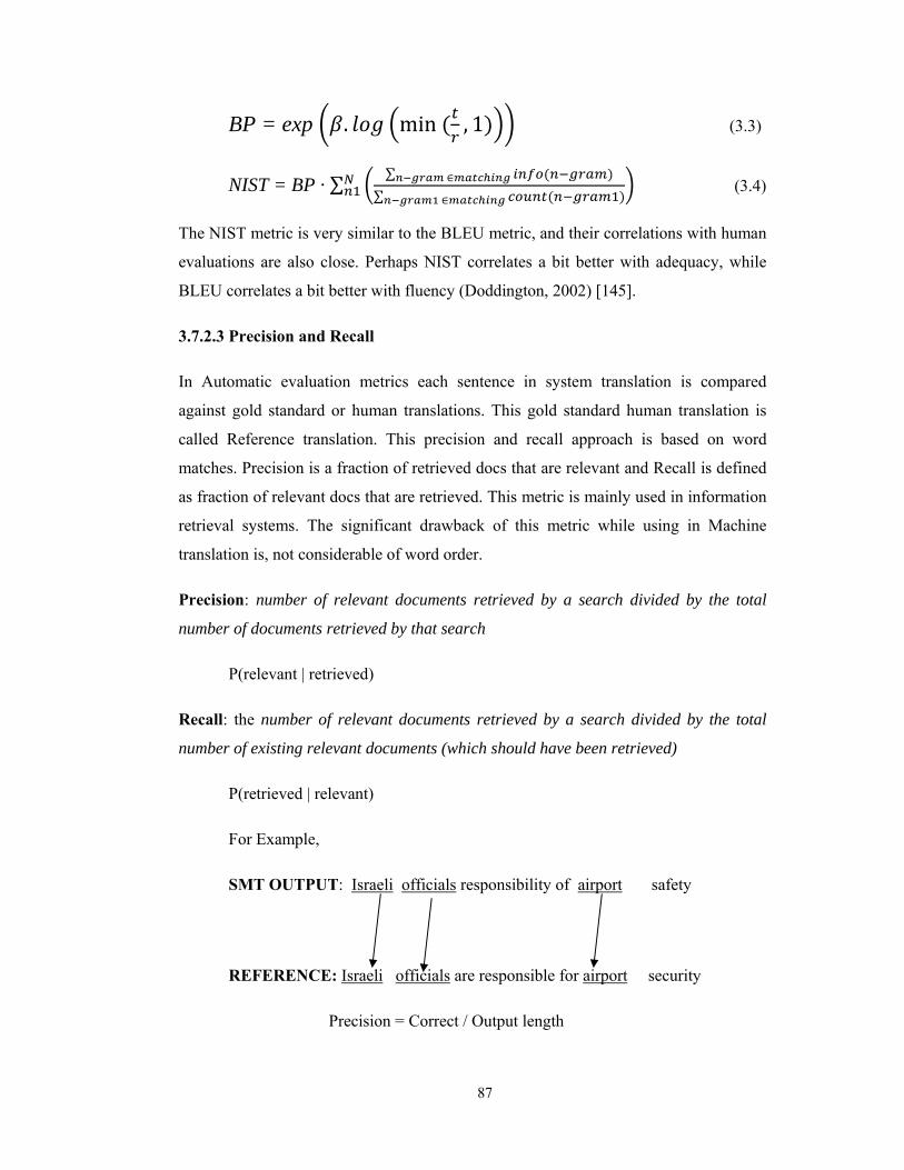
87
BP = exp . min , 1 (3.3)
NIST = BP · ∑∑
∑ (3.4)
The NIST metric is very similar to the BLEU metric, and their correlations with human
evaluations are also close. Perhaps NIST correlates a bit better with adequacy, while
BLEU correlates a bit better with fluency (Doddington, 2002) [145].
3.7.2.3 Precision and Recall
In Automatic evaluation metrics each sentence in system translation is compared
against gold standard or human translations. This gold standard human translation is
called Reference translation. This precision and recall approach is based on word
matches. Precision is a fraction of retrieved docs that are relevant and Recall is defined
as fraction of relevant docs that are retrieved. This metric is mainly used in information
retrieval systems. The significant drawback of this metric while using in Machine
translation is, not considerable of word order.
Precision: number of relevant documents retrieved by a search divided by the total
number of documents retrieved by that search
P(relevant | retrieved)
Recall: the number of relevant documents retrieved by a search divided by the total
number of existing relevant documents (which should have been retrieved)
P(retrieved | relevant)
For Example,
SMT OUTPUT: Israeli officials responsibility of airport safety
REFERENCE: Israeli officials are responsible for airport security
Precision = Correct / Output length
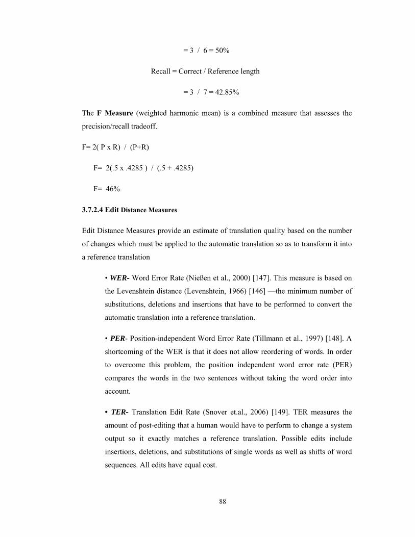
88
= 3 / 6 = 50%
Recall = Correct / Reference length
= 3 / 7 = 42.85%
The F Measure (weighted harmonic mean) is a combined measure that assesses the
precision/recall tradeoff.
F= 2( P x R) / (P+R)
F= 2(.5 x .4285 ) / (.5 + .4285)
F= 46%
3.7.2.4 Edit Distance Measures
Edit Distance Measures provide an estimate of translation quality based on the number
of changes which must be applied to the automatic translation so as to transform it into
a reference translation
• WER- Word Error Rate (Nießen et al., 2000) [147]. This measure is based on
the Levenshtein distance (Levenshtein, 1966) [146] —the minimum number of
substitutions, deletions and insertions that have to be performed to convert the
automatic translation into a reference translation.
• PER- Position-independent Word Error Rate (Tillmann et al., 1997) [148]. A
shortcoming of the WER is that it does not allow reordering of words. In order
to overcome this problem, the position independent word error rate (PER)
compares the words in the two sentences without taking the word order into
account.
• TER- Translation Edit Rate (Snover et.al., 2006) [149]. TER measures the
amount of post-editing that a human would have to perform to change a system
output so it exactly matches a reference translation. Possible edits include
insertions, deletions, and substitutions of single words as well as shifts of word
sequences. All edits have equal cost.
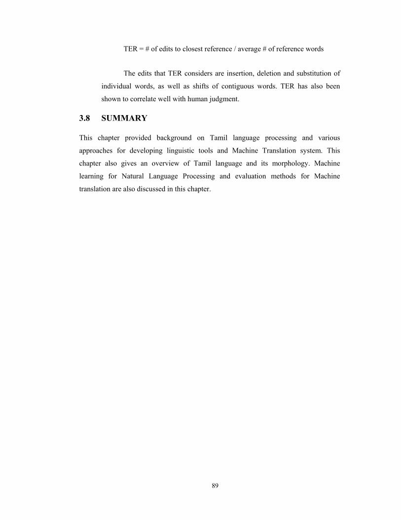
89
TER = # of edits to closest reference / average # of reference words
The edits that TER considers are insertion, deletion and substitution of
individual words, as well as shifts of contiguous words. TER has also been
shown to correlate well with human judgment.
3.8 SUMMARY
This chapter provided background on Tamil language processing and various
approaches for developing linguistic tools and Machine Translation system. This
chapter also gives an overview of Tamil language and its morphology. Machine
learning for Natural Language Processing and evaluation methods for Machine
translation are also discussed in this chapter.