27

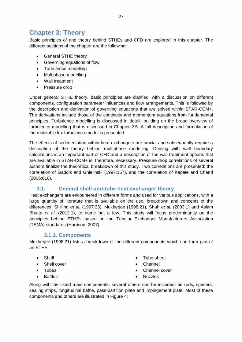
Chapter 3: Theory Basic principles of and theory behind STHEs and CFD are explored in this chapter. The

different sections of the chapter are the following:

General STHE theory

Governing equations of flow

Turbulence modelling

Multiphase modelling

Wall treatment

Pressure drop

Under general STHE theory, basic principles are clarified, with a discussion on different

components, configuration parameter influences and flow arrangements. This is followed by

the description and derivation of governing equations that are solved within STAR-CCM+.

The derivations include those of the continuity and momentum equations from fundamental

principles. Turbulence modelling is discussed in detail, building on the broad overview of

turbulence modelling that is discussed in Chapter 2.5. A full description and formulation of

the realizable k-ε turbulence model is presented.

The effects of sedimentation within heat exchangers are crucial and subsequently require a

description of the theory behind multiphase modelling. Dealing with wall boundary

calculations is an important part of CFD and a description of the wall treatment options that

are available in STAR-CCM+ is, therefore, necessary. Pressure drop correlations of several

authors finalize the theoretical breakdown of this study. Two correlations are presented: the

correlation of Gaddis and Gnielinski (1997:157), and the correlation of Kapale and Chand

(2006:610).

3.1. General shell-and-tube heat exchanger theory

Heat exchangers are encountered in different forms and used for various applications, with a

large quantity of literature that is available on the use, breakdown and concepts of the

differences: Shilling et al. (1997:33), Mukherjee (1998:21), Shah et al. (2003:1) and Aslam

Bhutta et al. (2012:1), to name but a few. This study will focus predominantly on the

principles behind STHEs based on the Tubular Exchanger Manufacturers Association

(TEMA) standards (Harrison, 2007).

3.1.1. Components

Mukherjee (1998:21) lists a breakdown of the different components which can form part of

an STHE:

Shell

Shell cover

Tubes

Baffles

Tube-sheet

Channel

Channel cover

Nozzles

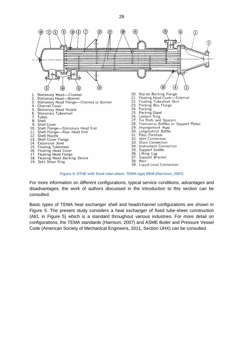
Along with the listed main components, several others can be included: tie rods, spacers,

sealing strips, longitudinal baffle, pass-partition plate and impingement plate. Most of these

components and others are illustrated in Figure 4:

28

Figure 4: STHE with fixed tube-sheet. TEMA-type BEM (Harrison, 2007)

For more information on different configurations, typical service conditions, advantages and

disadvantages, the work of authors discussed in the introduction to this section can be

consulted.

Basic types of TEMA heat exchanger shell and head/channel configurations are shown in

Figure 5. The present study considers a heat exchanger of fixed tube-sheet construction

(AEL in Figure 5) which is a standard throughout various industries. For more detail on

configurations, the TEMA standards (Harrison, 2007) and ASME Boiler and Pressure Vessel

Code (American Society of Mechanical Engineers, 2011, Section UHX) can be consulted.

29

Figure 5: TEMA classification of heat exchanger shells and headers/channels (Harrison, 2007)

3.1.2. Tube and baffle layouts

Mukherjee (1998:21) presented a discussion on the advantages and disadvantages of tube

layouts that were discussed in Chapter 1.3. General advantages and disadvantages of

triangular and square configurations consist of the following:

The triangular configuration has more tubes, resulting in better heat transfer.

30

For triangular patterns, typical tube pitches (1.25 times the tube outside diameter)

obstruct mechanical cleaning of external surfaces and are thus used for cleaner

shell-side conditions/processes.

Triangular patterns are generally suited for fixed tube-sheet arrangements due to the

arrangement’s requirement of clean shell-side flow conditions.

Rotated square arrangements offer better heat transfer/pressure drop ratios than

square arrangements and are better suited for low Reynolds number applications

(Re<2000).

Square patterns are suited for floating-head configurations.

Both the triangular and square arrangements can have a U-tube construction if the

shell-side flow conditions are clean and dirty, respectively.

The different baffle arrangements that were discussed in Chapter 1.3 have three main uses,

namely flow direction, tube support and vibration control. Shilling et al. (1997:33) stated that

the double-segmental configuration experiences a reduction in the cross-flow velocity. This

will also be the case for the disc-and-doughnut configuration. Both these configurations are

alternative solutions to pressure drop restrictions (Bell et al., 1983b).

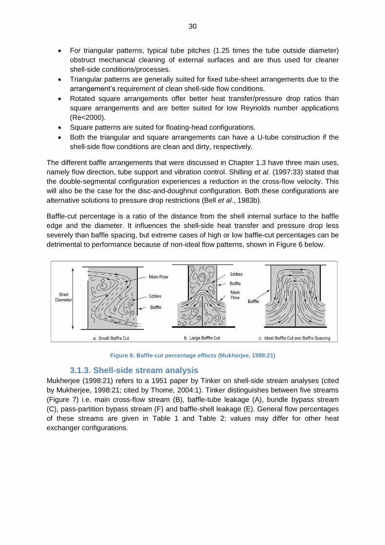
Baffle-cut percentage is a ratio of the distance from the shell internal surface to the baffle

edge and the diameter. It influences the shell-side heat transfer and pressure drop less

severely than baffle spacing, but extreme cases of high or low baffle-cut percentages can be

detrimental to performance because of non-ideal flow patterns, shown in Figure 6 below.

Figure 6: Baffle-cut percentage effects (Mukherjee, 1998:21)

3.1.3. Shell-side stream analysis

Mukherjee (1998:21) refers to a 1951 paper by Tinker on shell-side stream analyses (cited

by Mukherjee, 1998:21; cited by Thome, 2004:1). Tinker distinguishes between five streams

(Figure 7) i.e. main cross-flow stream (B), baffle-tube leakage (A), bundle bypass stream

(C), pass-partition bypass stream (F) and baffle-shell leakage (E). General flow percentages

of these streams are given in Table 1 and Table 2; values may differ for other heat

exchanger configurations.

31

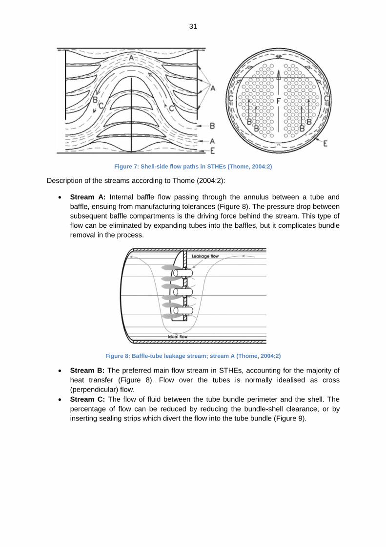
Figure 7: Shell-side flow paths in STHEs (Thome, 2004:2)

Description of the streams according to Thome (2004:2):

Stream A: Internal baffle flow passing through the annulus between a tube and

baffle, ensuing from manufacturing tolerances (Figure 8). The pressure drop between

subsequent baffle compartments is the driving force behind the stream. This type of

flow can be eliminated by expanding tubes into the baffles, but it complicates bundle

removal in the process.

Figure 8: Baffle-tube leakage stream; stream A (Thome, 2004:2)

Stream B: The preferred main flow stream in STHEs, accounting for the majority of

heat transfer (Figure 8). Flow over the tubes is normally idealised as cross

(perpendicular) flow.

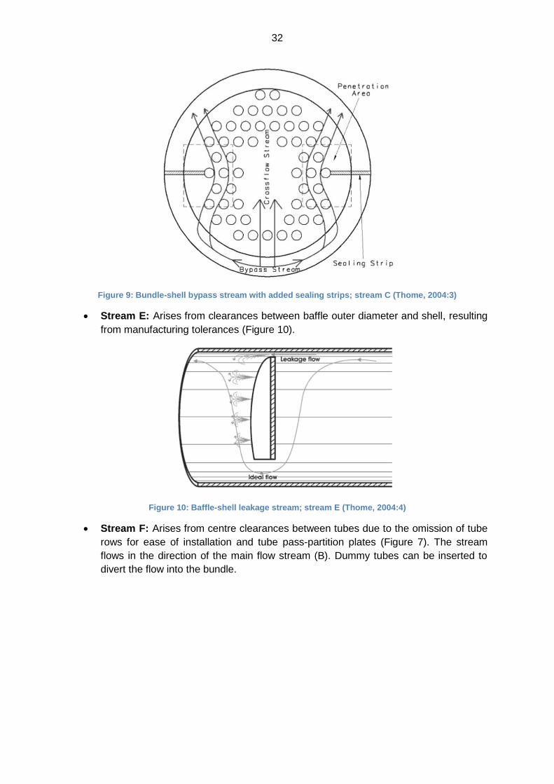
Stream C: The flow of fluid between the tube bundle perimeter and the shell. The

percentage of flow can be reduced by reducing the bundle-shell clearance, or by

inserting sealing strips which divert the flow into the tube bundle (Figure 9).

32

Figure 9: Bundle-shell bypass stream with added sealing strips; stream C (Thome, 2004:3)

Stream E: Arises from clearances between baffle outer diameter and shell, resulting

from manufacturing tolerances (Figure 10).

Figure 10: Baffle-shell leakage stream; stream E (Thome, 2004:4)

Stream F: Arises from centre clearances between tubes due to the omission of tube

rows for ease of installation and tube pass-partition plates (Figure 7). The stream

flows in the direction of the main flow stream (B). Dummy tubes can be inserted to

divert the flow into the bundle.

33

Flow fractions

Stream A 5.8%

Stream B 80.7%

Stream C 5.8%

Stream E 7.7%

Stream F 0.0%

Table 1: Flow fraction percentages (Lombaard, 2011)

Mohammadi (2011) cites the work of Palen and Taborek on shell-side flow fractions, in

which they use the Heat Transfer Research Institute’s (HTRI) stream analysis method. The

determined ranges for turbulent flow given in Table 1 vary from those given in Table 1:

Flow fractions

Stream A 9%-23%

Stream B 30%-65%

Stream C 15%-35%

Stream E 6%-21%

Stream F -

Table 2: Flow fractions in an STHE (Mohammadi, 2011)

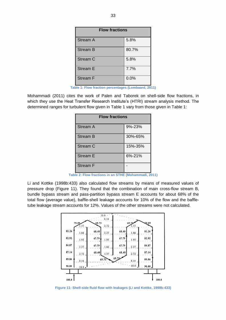
Li and Kottke (1998b:433) also calculated flow streams by means of measured values of

pressure drop (Figure 11). They found that the combination of main cross-flow stream B,

bundle bypass stream and pass-partition bypass stream E accounts for about 68% of the

total flow (average value), baffle-shell leakage accounts for 10% of the flow and the baffle-

tube leakage stream accounts for 12%. Values of the other streams were not calculated.

Figure 11: Shell-side fluid flow with leakages (Li and Kottke, 1998b:433)

34

Considering heat transfer, stream B is most efficient due to its cross-flow nature, streams A,

F and C are less effective because of reduced tube contact and stream E, encountering no

tubes, is minimally efficient.

Stream fractions are directly proportional to the flow resistances that are experienced by the

separate flow streams. These resistances are influenced by several factors:

Baffle spacing

Baffle-cut

Tube pitch

Tube arrangement

Number of lanes in the flow

direction

Flow direction lane width

Baffle-shell leakage area

Baffle-tube leakage area

Sealing strips and tie rod

placement

Fluid viscosity

3.2. Governing equations of flow

The derivation of the governing equations that is presented below was obtained from the

work by Rajagopalan (2004:21) and Anderson (1996:15).

3.2.1. Fluid motion description

There are two distinct ways of describing fluid in motion: the Lagrangian method (the fluid

element is described temporally and spatially) and the Eulerian method (the motion of the

fluid is described at every point within a control volume without considering individual

elements). Within the Eulerian framework, a distinct property (γ) of the field can be described

unsteadily in three-dimensional space by the following function:

( ) (3.1)

γ is any property such as temperature, pressure, density, velocity etc.

q1 is the 1stcoordinate of three-dimensional space.

q2 is the 2ndcoordinate of three-dimensional space.

q3 is the 3rd coordinate of three-dimensional space.

t is time.

Note that the history and spatial variation of any property γ can be described by fixing either

the spacial or temporal variables respectively. In a Cartesian reference frame, Equation (3.1)

above will be:

( ) (3.2)

3.2.2. Substantial/Total derivative

The substantial derivative provides a means of describing the time rate of change of a

property of an element in a Lagrangian framework in terms of the spatial Eulerian framework

at a specific position. The time derivative of the variable γ can be described as follows:

(3.3)

but

35

(3.4)

where the time rate of change of a spatial coordinate x is defined as the u-velocity

component of velocity field ; the same applies to the y- and z-direction. Substituting this into

Equation (3.3) results in:

(3.5)

or

(3.6)

The left-hand side (LHS) of Equation (3.6) is the total derivative or time rate of

change of a fluid element, described in a Lagrangian framework.

The first term on the right-hand side (RHS) is the convective derivative. This is the

time rate of change of the property due to the fluid movement between two points,

expressed in an Eulerian framework.

The second term on the RHS is the local derivative. It is the temporal rate of change

at a fixed point, described in an Eulerian framework.

3.2.3. Reynolds’ transport theorem

Describing the laws of physics in terms of a fixed region of space, with several elements

occupying this region at any time, is said to be an Eulerian reference frame. A Lagrangian

reference frame describes the laws for specific particles as they move. Within the

Lagrangian reference frame the conservation laws are more easily applied, whereas the

description in the Eulerian frame is preferred. Difficulties arise because of continuous fluid

distortion and deformation, in effect hampering the identification and observation of a

particular mass of fluid. Normally, the focus is placed on the effect of fluid motion and not a

particular mass.

The difficulties are overcome by means of the Reynolds’ transport theorem. The theorem

describes the relation between Lagrangian and Eulerian frameworks in terms of a specific

property. An extensive property (λ) is converted to an intensive property (γ) through Equation

(3.7):

) ∫ ∫

(3.7)

This leads to:

( )

(∫

)

(∫

) ∫ ( )

(3.8)

The LHS Equation (3.8) is the rate of change of any extensive property.

36

The first term of the RHS of the equation is the time rate of change of the extensive

property within the control volume, evaluated by a fixed observer.

The second term of the RHS is the rate of efflux of the extensive property through the

boundaries of the control volume.

is the velocity that is measured relative to the control volume.

is the density of the system.

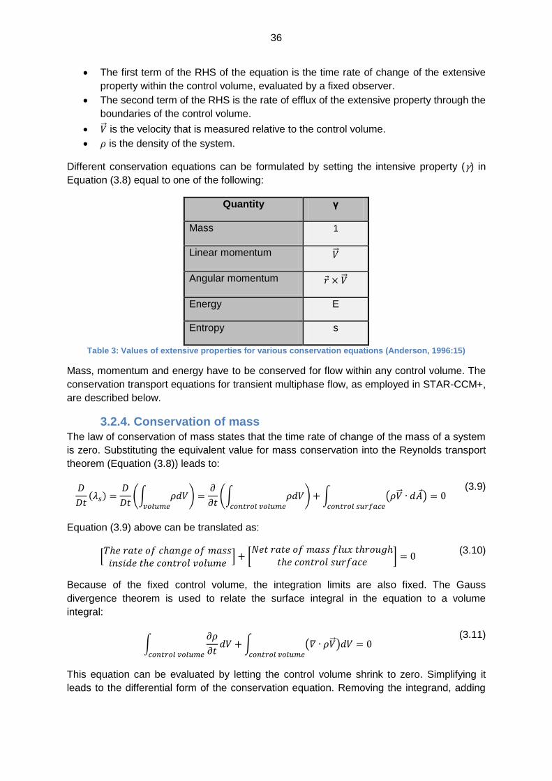
Different conservation equations can be formulated by setting the intensive property (γ) in

Equation (3.8) equal to one of the following:

Quantity γ

Mass 1

Linear momentum

Angular momentum

Energy E

Entropy s

Table 3: Values of extensive properties for various conservation equations (Anderson, 1996:15)

Mass, momentum and energy have to be conserved for flow within any control volume. The

conservation transport equations for transient multiphase flow, as employed in STAR-CCM+,

are described below.

3.2.4. Conservation of mass

The law of conservation of mass states that the time rate of change of the mass of a system

is zero. Substituting the equivalent value for mass conservation into the Reynolds transport

theorem (Equation (3.8)) leads to:

( )

(∫

)

(∫

) ∫ ( )

(3.9)

Equation (3.9) above can be translated as:

[

] [

]

(3.10)

Because of the fixed control volume, the integration limits are also fixed. The Gauss

divergence theorem is used to relate the surface integral in the equation to a volume

integral:

∫

∫ ( )

(3.11)

This equation can be evaluated by letting the control volume shrink to zero. Simplifying it

leads to the differential form of the conservation equation. Removing the integrand, adding

37

phase denoting subscripts to all variables and multiplying throughout with the

concentration/volume fraction scalar, the equation transforms to:

( ) ( )

(3.12)

with:

∑

(3.13)

where:

αi is the volume fraction;

ρi is the density;

vi is the velocity; and

subscript i denotes the generic phase.

3.2.5. Conservation of momentum

The momentum conservation equation is directly derived from Newton’s second law. The

same method of derivation of the continuity equation can be followed, but the preferred

method is fundamentally oriented and fully descriptive (Anderson, 1996:15). The momentum

equation was derived in non-conservative form (Lagrangian framework) and be converted to

the conservative form (Eulerian framework). Derivation originates from Newton’s 2nd law in

the Cartesian x-direction:

(3.14)

Fx is the scalar x-component of the forces working on the fluid element.

m is the mass of the fluid element.

ax is the scalar x-component of the acceleration that is experienced by the fluid

element.

Two types of forces act on the element, namely body forces and surface forces. Body forces

act directly on the volumetric mass from a distance, whilst surface forces originate at the

surface of the fluid element. Surface forces have two constituents: distributed pressure due

to the environment (surrounding fluid), and shear and normal stress distributions due to

viscosity-related ‘friction’, arising from the movement of the surrounding fluid. The body force

is described in Equation (3.15):

[

]

( ) (3.15)

is the x-component of the body force .

( ) is the differential volume of the element.

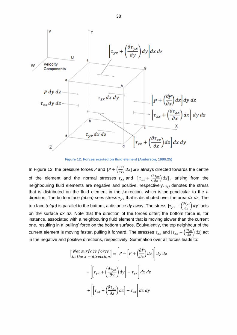
Surface forces acting on the fluid element in Cartesian coordinates are described in Figure

12. Velocity vectors u, v and w increase in the positive axis directions.

38

Figure 12: Forces exerted on fluid element (Anderson, 1996:25)

In Figure 12, the pressure forces and [ (

) are always directed towards the centre

of the element and the normal stresses and [ (

) , arising from the

neighbouring fluid elements are negative and positive, respectively. denotes the stress

that is distributed on the fluid element in the j-direction, which is perpendicular to the i-

direction. The bottom face (abcd) sees stress that is distributed over the area dx dz. The

top face (efgh) is parallel to the bottom, a distance dy away. The stress [ (

) acts

on the surface dx dz. Note that the direction of the forces differ; the bottom force is, for

instance, associated with a neighbouring fluid element that is moving slower than the current

one, resulting in a ‘pulling’ force on the bottom surface. Equivalently, the top neighbour of the

current element is moving faster, pulling it forward. The stresses and [ (

) act

in the negative and positive directions, respectively. Summation over all forces leads to:

[

] [ [ (

) ]]

[[ (

) ] ]

[[ (

) ] ]

39

[[ (

) ] ]

(3.16)

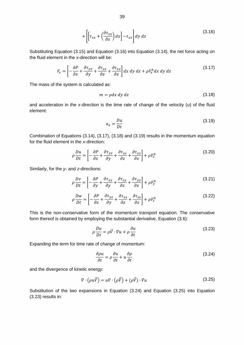
Substituting Equation (3.15) and Equation (3.16) into Equation (3.14), the net force acting on

the fluid element in the x-direction will be:

[

]

(3.17)

The mass of the system is calculated as:

(3.18)

and acceleration in the x-direction is the time rate of change of the velocity (u) of the fluid

element:

(3.19)

Combination of Equations (3.14), (3.17), (3.18) and (3.19) results in the momentum equation

for the fluid element in the x-direction:

[

]

(3.20)

Similarly, for the y- and z-directions:

[

]

(3.21)

[

]

(3.22)

This is the non-conservative form of the momentum transport equation. The conservative

form thereof is obtained by employing the substantial derivative, Equation (3.6):

(3.23)

Expanding the term for time rate of change of momentum:

(3.24)

and the divergence of kinetic energy:

( ) ( ) ( ) (3.25)

Substitution of the two expansions in Equation (3.24) and Equation (3.25) into Equation

(3.23) results in:

40

( ) ( )

(3.26)

Rewritten:

[

( )] ( )

(3.27)

The term in brackets corresponds with the continuity equation, which is equal to zero. The

resulting Navier-Stokes equations in conservative form for Cartesian coordinates are:

( ) [

]

(3.28)

( ) [

]

(3.29)

( ) [

]

(3.30)

Finally, all nine stress variables can be related to velocity gradients in the fluid by means of

equations for Newtonian fluids, developed by Isaac Newton (cited by Anderson, 1996:15):

(3.31)

(

) (

) (

)

(3.32)

is the molecular viscosity.

is the bulk viscosity.

Substituting these stress relations into the conservative form momentum equations will lead

to the momentum equation that is used in STAR-CCM+. Several modifications are made to

the equations. Similar to the continuity equation, a volume fraction variable is added to all

terms; they are all described in terms of the specific phase that is designated by the

subscript i; and the body forces are expanded into a gravity term, combined stress terms and

inter-phase momentum transfer terms:

( ) ( ) [ (

)]

(3.33)

P is the pressure of all phases.

g is the gravity vector.

τim and τi

t are the molecular and turbulent stresses, respectively.

Mij is the inter-phase momentum transfer per unit volume, discussed in Chapter 3.4.

41

3.3. Turbulence modelling

3.3.1. General overview

The reasoning behind the selection of the realizable k-ε turbulence model was discussed in

Chapter 2.5. The theory behind the model is subsequently presented below, adapted from

the STAR-CCM+ User Guide v.6.06 (2011:2851).

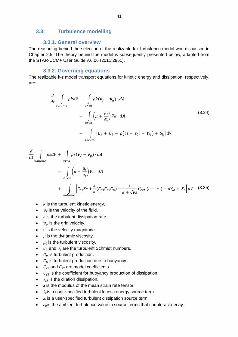
3.3.2. Governing equations

The realizable k-ε model transport equations for kinetic energy and dissipation, respectively,

are:

∫

∫ ( )

∫ (

)

∫ [ (( ) ) ]

(3.34)

∫

∫ ( )

∫ (

)

∫ [

( )

√ ( ) ]

(3.35)

k is the turbulent kinetic energy.

is the velocity of the fluid.

ε is the turbulent dissipation rate.

is the grid velocity.

is the velocity magnitude

is the dynamic viscosity.

is the turbulent viscosity.

and are the turbulent Schmidt numbers.

is turbulent production.

is turbulent production due to buoyancy.

and are model coefficients.

is the coefficient for buoyancy production of dissipation.

is the dilation dissipation.

S is the modulus of the mean strain rate tensor.

Sk is a user-specified turbulent kinetic energy source term.

Sε is a user-specified turbulent dissipation source term.

ε0 is the ambient turbulence value in source terms that counteract decay.

42

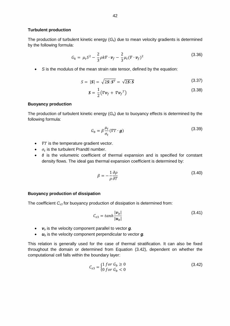
Turbulent production

The production of turbulent kinetic energy (Gk) due to mean velocity gradients is determined

by the following formula:

( )

(3.36)

S is the modulus of the mean strain rate tensor, defined by the equation:

| | √ √ (3.37)

(

) (3.38)

Buoyancy production

The production of turbulent kinetic energy (Gb) due to buoyancy effects is determined by the

following formula:

( ) (3.39)

is the temperature gradient vector.

is the turbulent Prandtl number.

β is the volumetric coefficient of thermal expansion and is specified for constant

density flows. The ideal gas thermal expansion coefficient is determined by:

(3.40)

Buoyancy production of dissipation

The coefficient Cε3 for buoyancy production of dissipation is determined from:

| |

| |

(3.41)

vb is the velocity component parallel to vector g.

ub is the velocity component perpendicular to vector g.

This relation is generally used for the case of thermal stratification. It can also be fixed

throughout the domain or determined from Equation (3.42), dependent on whether the

computational cell falls within the boundary layer:

{

(3.42)

43

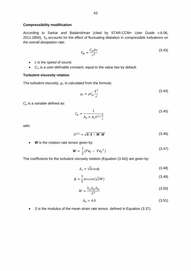
Compressibility modification

According to Sarkar and Balakrishnan (cited by STAR-CCM+ User Guide v.6.06,

2011:2850), ΥM accounts for the effect of fluctuating dilatation in compressible turbulence on

the overall dissipation rate:

(3.43)

c is the speed of sound.

Cm is a user-definable constant, equal to the value two by default.

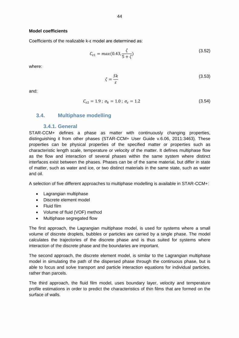
Turbulent viscosity relation

The turbulent viscosity, μt, is calculated from the formula:

(3.44)

Cμ is a variable defined as:

( )

(3.45)

with:

( ) √ (3.46)

W is the rotation rate tensor given by:

(

) (3.47)

The coefficients for the turbulent viscosity relation (Equation (3.44)) are given by:

√ (3.48)

(√ )

(3.49)

(3.50)

(3.51)

S is the modulus of the mean strain rate tensor, defined in Equation (3.37).

44

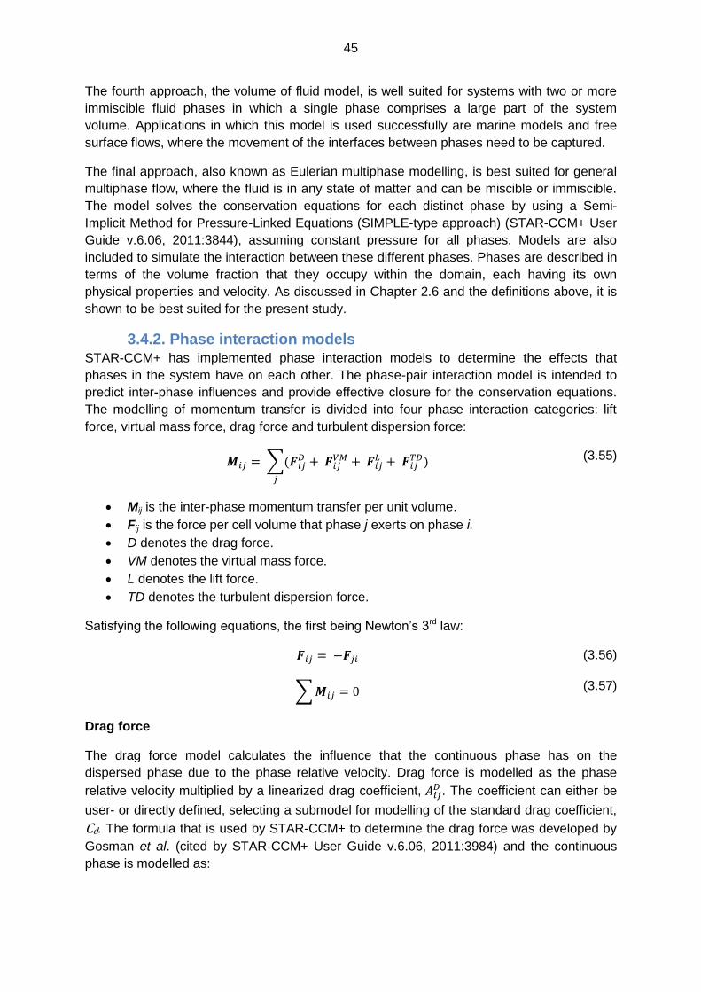
Model coefficients

Coefficients of the realizable k-ε model are determined as:

(

)

(3.52)

where:

(3.53)

and:

(3.54)

3.4. Multiphase modelling

3.4.1. General

STAR-CCM+ defines a phase as matter with continuously changing properties,

distinguishing it from other phases (STAR-CCM+ User Guide v.6.06, 2011:3463). These

properties can be physical properties of the specified matter or properties such as

characteristic length scale, temperature or velocity of the matter. It defines multiphase flow

as the flow and interaction of several phases within the same system where distinct

interfaces exist between the phases. Phases can be of the same material, but differ in state

of matter, such as water and ice, or two distinct materials in the same state, such as water

and oil.

A selection of five different approaches to multiphase modelling is available in STAR-CCM+:

Lagrangian multiphase

Discrete element model

Fluid film

Volume of fluid (VOF) method

Multiphase segregated flow

The first approach, the Lagrangian multiphase model, is used for systems where a small

volume of discrete droplets, bubbles or particles are carried by a single phase. The model

calculates the trajectories of the discrete phase and is thus suited for systems where

interaction of the discrete phase and the boundaries are important.

The second approach, the discrete element model, is similar to the Lagrangian multiphase

model in simulating the path of the dispersed phase through the continuous phase, but is

able to focus and solve transport and particle interaction equations for individual particles,

rather than parcels.

The third approach, the fluid film model, uses boundary layer, velocity and temperature

profile estimations in order to predict the characteristics of thin films that are formed on the

surface of walls.

45

The fourth approach, the volume of fluid model, is well suited for systems with two or more

immiscible fluid phases in which a single phase comprises a large part of the system

volume. Applications in which this model is used successfully are marine models and free

surface flows, where the movement of the interfaces between phases need to be captured.

The final approach, also known as Eulerian multiphase modelling, is best suited for general

multiphase flow, where the fluid is in any state of matter and can be miscible or immiscible.

The model solves the conservation equations for each distinct phase by using a Semi-

Implicit Method for Pressure-Linked Equations (SIMPLE-type approach) (STAR-CCM+ User

Guide v.6.06, 2011:3844), assuming constant pressure for all phases. Models are also

included to simulate the interaction between these different phases. Phases are described in

terms of the volume fraction that they occupy within the domain, each having its own

physical properties and velocity. As discussed in Chapter 2.6 and the definitions above, it is

shown to be best suited for the present study.

3.4.2. Phase interaction models

STAR-CCM+ has implemented phase interaction models to determine the effects that

phases in the system have on each other. The phase-pair interaction model is intended to

predict inter-phase influences and provide effective closure for the conservation equations.

The modelling of momentum transfer is divided into four phase interaction categories: lift

force, virtual mass force, drag force and turbulent dispersion force:

∑(

)

(3.55)

Mij is the inter-phase momentum transfer per unit volume.

Fij is the force per cell volume that phase j exerts on phase i.

D denotes the drag force.

VM denotes the virtual mass force.

L denotes the lift force.

TD denotes the turbulent dispersion force.

Satisfying the following equations, the first being Newton’s 3rd law:

(3.56)

∑ (3.57)

Drag force

The drag force model calculates the influence that the continuous phase has on the

dispersed phase due to the phase relative velocity. Drag force is modelled as the phase

relative velocity multiplied by a linearized drag coefficient, . The coefficient can either be

user- or directly defined, selecting a submodel for modelling of the standard drag coefficient,

Cd. The formula that is used by STAR-CCM+ to determine the drag force was developed by

Gosman et al. (cited by STAR-CCM+ User Guide v.6.06, 2011:3984) and the continuous

phase is modelled as:

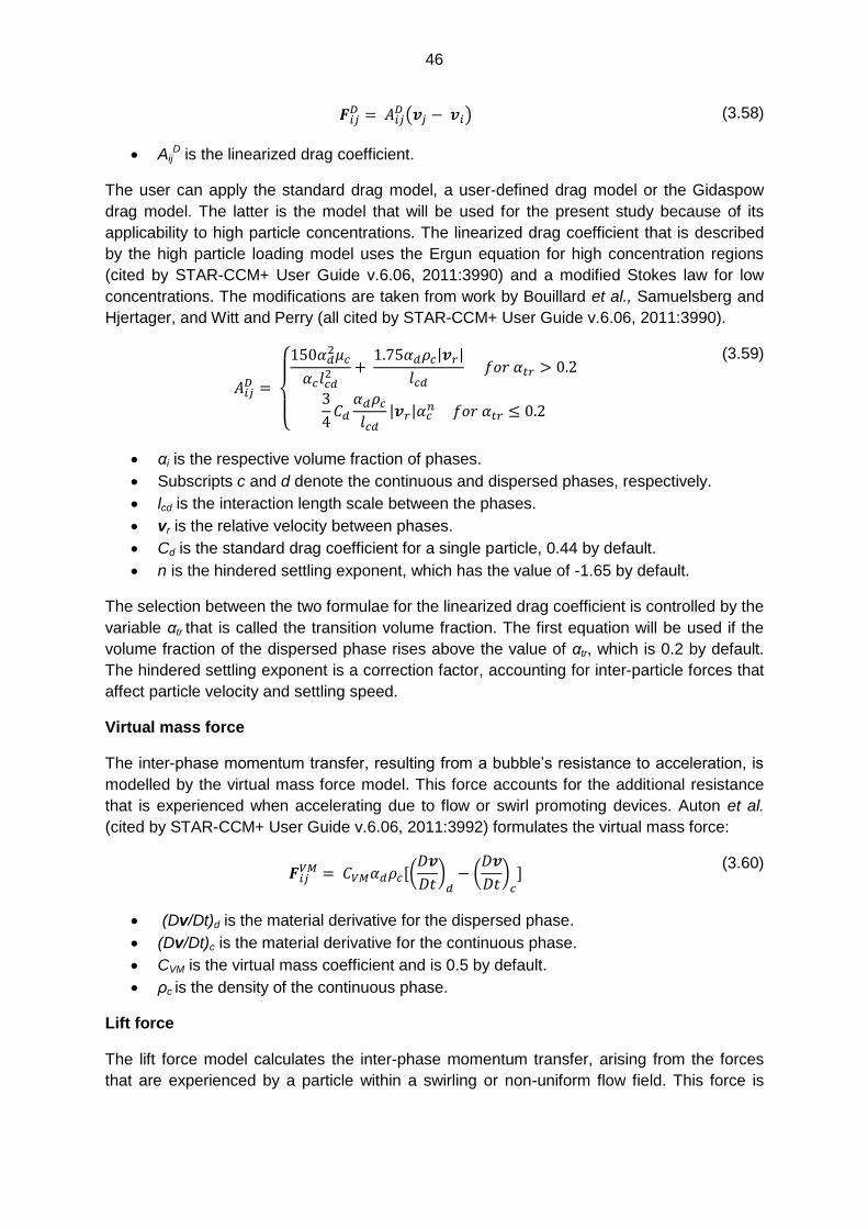
46

( ) (3.58)

AijD is the linearized drag coefficient.

The user can apply the standard drag model, a user-defined drag model or the Gidaspow

drag model. The latter is the model that will be used for the present study because of its

applicability to high particle concentrations. The linearized drag coefficient that is described

by the high particle loading model uses the Ergun equation for high concentration regions

(cited by STAR-CCM+ User Guide v.6.06, 2011:3990) and a modified Stokes law for low

concentrations. The modifications are taken from work by Bouillard et al., Samuelsberg and

Hjertager, and Witt and Perry (all cited by STAR-CCM+ User Guide v.6.06, 2011:3990).

{

| |

| |

(3.59)

αi is the respective volume fraction of phases.

Subscripts c and d denote the continuous and dispersed phases, respectively.

lcd is the interaction length scale between the phases.

vr is the relative velocity between phases.

Cd is the standard drag coefficient for a single particle, 0.44 by default.

n is the hindered settling exponent, which has the value of -1.65 by default.

The selection between the two formulae for the linearized drag coefficient is controlled by the

variable αtr that is called the transition volume fraction. The first equation will be used if the

volume fraction of the dispersed phase rises above the value of αtr, which is 0.2 by default.

The hindered settling exponent is a correction factor, accounting for inter-particle forces that

affect particle velocity and settling speed.

Virtual mass force

The inter-phase momentum transfer, resulting from a bubble’s resistance to acceleration, is

modelled by the virtual mass force model. This force accounts for the additional resistance

that is experienced when accelerating due to flow or swirl promoting devices. Auton et al.

(cited by STAR-CCM+ User Guide v.6.06, 2011:3992) formulates the virtual mass force:

(

)

(

)

(3.60)

(Dv/Dt)d is the material derivative for the dispersed phase.

(Dv/Dt)c is the material derivative for the continuous phase.

CVM is the virtual mass coefficient and is 0.5 by default.

ρc is the density of the continuous phase.

Lift force

The lift force model calculates the inter-phase momentum transfer, arising from the forces

that are experienced by a particle within a swirling or non-uniform flow field. This force is

47

perpendicular to the relative velocity between the phases. Once again, Auton et al. (cited by

STAR-CCM+ User Guide v.6.06, 2011:3992) describes the lift force:

( ) (3.61)

CL is the lift coefficient, which is either user definable or equal to 0.25 by default, as

prescribed by Lance et al. (cited by STAR-CCM+ User Guide v.6.06, 2011:3992).

Turbulent dispersion force

The turbulent dispersion force model accounts for the interaction of the dispersed phase with

the system turbulent eddies in the continuous phase. Modelling follows:

(

)

(

)

(3.62)

νtc is the continuous phase turbulent kinematic viscosity.

σt is the turbulent Prandtl number.

Solid pressure force

The solid pressure force is required to model the resistance of an unrealistic formation of

solid packing fractions. The equation is only incorporated into the momentum equation of the

solid phase and the value thereof increases until the volume fraction of solids reaches

maximum packing limit. The equation is formulated as:

( )

∑

[ ( ∑

)] (∑

)

(3.63)

where:

is the cell-packing limit;

is the maximum cell-packing limit;

is the number of particle phases; and

Asp is the model constant, -600 by default.

The value of is user definable and is by default set to the maximum packing limit for

spherical particles of 0.624.

3.5. Wall treatment

3.5.1. Introduction

The use of wall treatment is entirely dependent on the near-wall mesh resolution and

location of the wall-adjacent cell within the turbulent boundary layer. The STAR-CCM+ User

Guide v.6.06 (2011:2768) describes the term ’wall treatment’ as a set of assumptions that

are made in order to model near-wall turbulent flow. The wall treatment options are designed

to be used in conjunction with a turbulence model, based on specific assumptions for

variables that are required for wall boundaries.

48

Chung (2002:688) states that the purpose of wall treatment is to lessen computational

requirements that result from the fine mesh requirement of wall-bounded flows. Due to the

distortion of the free-stream velocity profile that results in the boundary layer, velocity

gradients become very large near the wall, requiring a fine mesh resolution to resolve the

arising profile in order to obtain the necessary boundary conditions. Wall treatment alleviates

this problem by making certain assumptions with respect to the gradient. Depending on

whether the wall-adjacent cell centroid falls within the viscous-dominated region of the

boundary layer where the non-dimensional wall distance y+ ≤ 11.63 (Shyy et al., 1997:171;

Date, 2005:130), the low Reynolds number approach will be used and similarly, if the

centroid falls within the log-layer, y+ ≥ 30, the standard wall function approach will be used.

The intermediate or buffer region, 11.63 ≤ y+ ≤ 30, is described by a blended wall-law.

3.5.2. Wall-laws

A wall-law is a mathematical description of equilibrium mean flow quantities, such as

temperature, velocity and species concentration, in turbulent boundary layers. The wall-law

approach is used to circumvent the solution of turbulence model equations close to the wall

in order to avoid numerical problems and fine mesh resolutions in a viscous-dominated

region. Certain assumptions are made in the process. The first one is with respect to the

turbulence, velocity and scalar quantity distributions and profiles. The second is that the

chosen turbulence model is only valid and resolved outside of the viscous boundary layer.

This also makes it unnecessary to modify the turbulence equations in order to account for

low Reynolds number effects. The last one is that, in order to avoid the difficulty of solving

the equations of the chosen turbulence model, the near-wall cell centroid is assumed to fall

within the logarithmic region of the boundary layer. The mean flow quantities that are

described above are thus fixed in the log-layer region, some distance from the wall (Hallback

et al., 1996:143; Chung, 2002:688).

The STAR-CCM+ makes use of two wall-law types that are not user selectable:

Standard wall-laws, where the slope of the flow quantity is discontinuous between the

turbulent and laminar profiles.

Blended wall-laws, where the turbulent and laminar profiles are smoothly blended

together in a buffer region.

The laws are chosen, based on the turbulence model behaviour; those which contain or

behave as if they contain damping functions will use the blended-type. The High-y+ wall

treatments will make use of the standard wall-law.

3.5.3. Wall-law formulations

The wall-laws are set up to provide the non-dimensional velocity u+ and its first derivative as

a function of the non-dimensional wall distance y+ and other quantities (turbulent and

molecular Prandtl numbers). The non-dimensional quantities have the following relations:

(3.64)

(3.65)

y+ is the non-dimensional wall coordinate/distance.

49

yn is the normal distance from the wall to the wall-cell centroid.

u* is the reference velocity, derived from a turbulence quantity that is specific to the

chosen turbulence model.

v is the kinematic viscosity.

u+ is the non-dimensional wall-parallel velocity.

up is the component of wall-cell velocity, parallel to the wall.

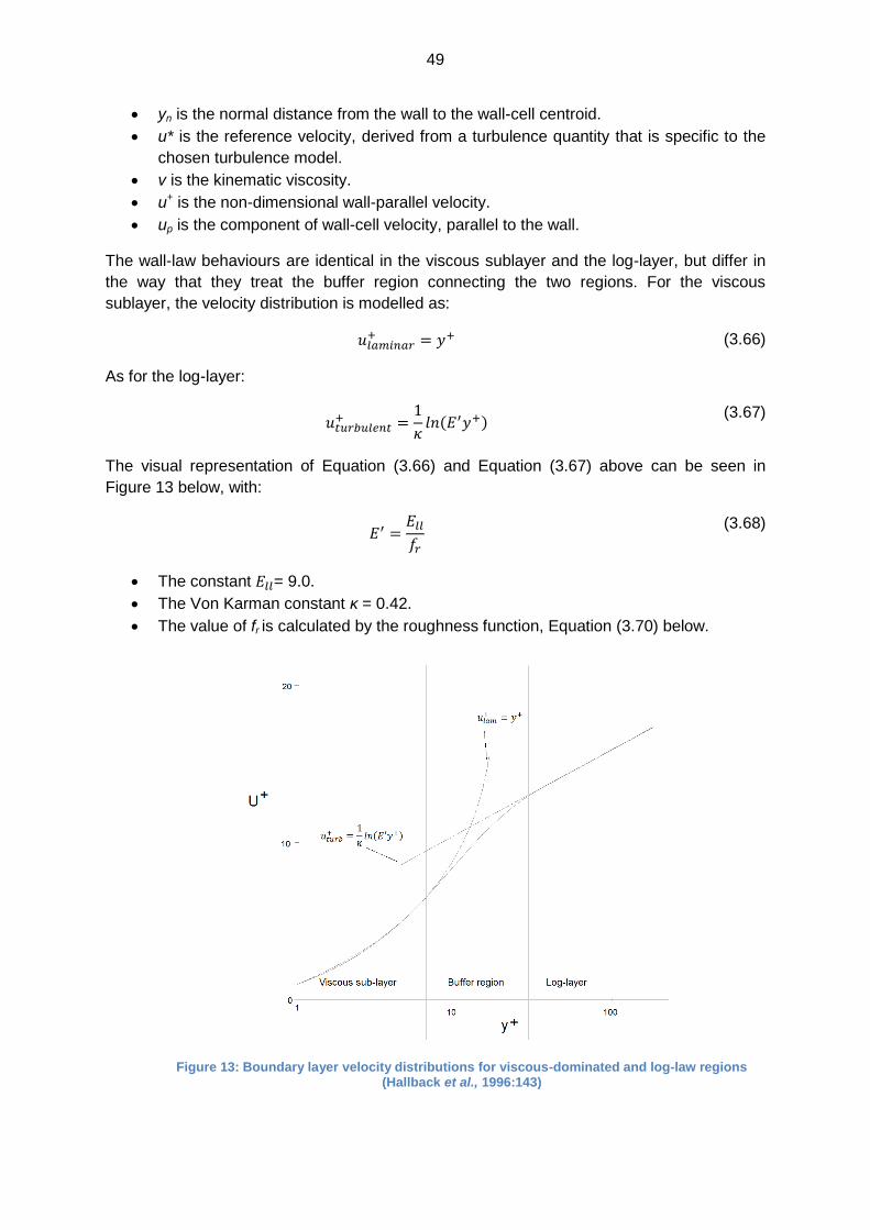
The wall-law behaviours are identical in the viscous sublayer and the log-layer, but differ in

the way that they treat the buffer region connecting the two regions. For the viscous

sublayer, the velocity distribution is modelled as:

(3.66)

As for the log-layer:

( )

(3.67)

The visual representation of Equation (3.66) and Equation (3.67) above can be seen in

Figure 13 below, with:

(3.68)

The constant = 9.0.

The Von Karman constant κ = 0.42.

The value of fr is calculated by the roughness function, Equation (3.70) below.

Figure 13: Boundary layer velocity distributions for viscous-dominated and log-law regions (Hallback et al., 1996:143)

50

Roughness function

The log-law coefficient E` in Equation (3.68) is a function of the roughness parameter:

(3.69)

The variable r in Equation (3.69) is the equivalent sand-grain roughness height. The

equation for roughness function is obtained from Cebeci and Bradshaw (cited by STAR-

CCM+ User Guide v.6.06, 2011:2778):

{

[ (

) ]

(3.70)

(

(

(

))

(3.71)

where:

is 0 by default;

is 0.253 by default;

is 2.25 by default; and

is 90 by default.

The transition between the formulae in Equation (3.70) is dependent on the value of . The

first, second and third formula is used if the value of falls below , in between or

above , respectively.

Standard wall-law

The standard wall-law has relations for the velocity distribution, having a discontinuous

slope:

{

(3.72)

The value of ym+, the layer-intersectional value for the non-dimensional wall distance, is

found by making use of the Newtonian iteration procedure.

Blended wall-law

This formulation smoothly blends the viscous and logarithmic layers. For momentum,

Reichards’s law (cited by STAR-CCM+ User Guide v.6.06, 2011:2777) is used:

( ) [ (

)

( )]

(3.73)

with:

51

(

)

(3.74)

(

)

(3.75)

3.5.4. Wall treatment selection A wall function approach describes the boundary conditions that are required by the

continuum equations in terms of a set of mathematical relations. These assumptions reduce

the amount of numerical problems, computational time and resources that are required to

resolve near-wall flow by reducing the mesh resolution requirement in the area of viscous

flow domination, as stated above.

The low Reynolds number approach is applied when the resolution of the viscous sublayer

velocity profile is possible through the use of a turbulence model and a sufficiently fine mesh.

Typically, the approach is used in separation regions and turbulent boundary layer flows at

lower Reynolds numbers (Hallback et al., 1996:145).

The following six different wall treatment options which are appropriate for the k-ε model

family are available in STAR-CCM+, although availability is subject to the chosen k-ε

turbulence model:

The high-y+ wall treatment, which has a wall function approach.

The low-y+ wall treatment, which is used for low Reynolds number turbulence models

with the viscous sublayer resolved.

The all-y+ wall treatment, which is a fusion between the high-y+ treatment in coarse

meshes and the low-y+ treatment for fine meshes, producing reasonably accurate

answers for a wide range of mesh sizes.

The two-layer all-y+ wall treatment, which is similar to the all-y+ treatment above, but

prescribes a boundary condition for turbulent dissipation.

The multiphase high-y+ wall treatment, which makes assumptions concerning the

wall stress distribution between phases. The assumptions that are made are that the

contact area of each phase is in proportion to its volume fraction in the wall-adjacent

cell and that a single-phase wall treatment is applied to each phase within its contact

area.

The multiphase two-layer all-y+ wall treatment, which is similar to both the multiphase

and two-layer treatment above in the way in which it describes the phase wall stress

and turbulent dissipation rate boundary condition.

3.5.5. Two-layer approach

As discussed in Chapter 2.5, the selected wall treatment option is the two-layer model. It

simplifies calculations for the turbulent dissipation rate in the near-wall region and solves the

turbulent kinetic energy equation throughout the computational domain. It is in effect a one-

equation model that algebraically prescribes the value for the turbulent dissipation rate as a

function of the wall distance.

The model is parameterized as a length scale function and a turbulent viscosity ratio function

respectively:

52

( ) (3.76)

( ) (3.77)

The turbulent Reynolds number is given by:

√

(3.78)

The dissipation rate equation is described by:

(3.79)

In the near-wall region, Jongen (cited by STAR-CCM+ User Guide v.6.06, 2011:2862)

suggested the following blending function to accomplish the combination of the two-layer

and full two-equation model:

[ (

)]

(3.80)

φ is the blending parameter that is used in Equation (3.82).

Rey* defines the limit of applicability of the two-layer formulation and the value is set

equal to 60 in STAR-CCM+.

Abl determines the width of the blending function. A relation for Abl is defined in such

a way that φ will be within 1% of its far-field value for a given variation of ΔRey. The

value for this is ΔRey = 10and relation between the two constants is:

| |

(3.81)

Determining the value for turbulent viscosity is done in the following way:

| ( ) (

)

(3.82)

Wolfstein model

Wolfstein (cited by STAR-CCM+ User Guide v.6.06, 2011:2862) presented the following

method of modelling turbulent viscosity and the length scale:

[ (

)]

(3.83)

(3.84)

(3.85)

Constant Cv = 0.09.

Turbulent viscosity is described by:

53

[ (

)]

(3.86)

Constant Aμ = 70.

3.6. Pressure drop

3.6.1. Gaddis and Gnielinski

A method for the determination of pressure drop within an STHE is presented, obtained from

the work of Gaddis and Gnielinski (1997:159). This method was developed in equation form,

similar to the calculations of the VDI-Wärmeatlas (cited by Gaddis and Gnielinski, 1997:159).

The full correlation will not be presented in this text, but will be thoroughly implemented. The

overall shell-side pressure drop equation is:

( ) (3.87)

with:

the interior cross-flow pressure drop;

the end cross-flow region pressure drop;

the window section pressure drop;

the inlet and outlet nozzle pressure drop; and

Nb the number of baffles.

Several assumptions are made in the calculation procedure. The pressure drop in

subsequent compartments are assumed to be constant along the heat exchanger length.

Mean values for the fluid properties are assigned, assuming that property changes as well

as the influence of different baffle compartment lengths are negligible.

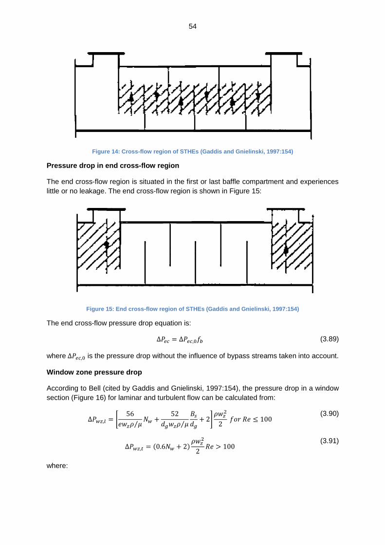
Cross-flow pressure drop

The cross-flow section is the tube section that experiences perpendicular flow and is situated

between planes that are tangent to the baffle top edges of adjacent baffles (Figure 14). The

equation for cross-flow pressure drop is:

(3.88)

where:

is the pressure drop over an ideal tube bank, without leakage streams;

is a correction factor for the influence of leakage streams; and

is a correction factor for the influence of bypass streams.

54

Figure 14: Cross-flow region of STHEs (Gaddis and Gnielinski, 1997:154)

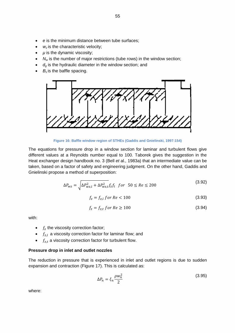
Pressure drop in end cross-flow region

The end cross-flow region is situated in the first or last baffle compartment and experiences

little or no leakage. The end cross-flow region is shown in Figure 15:

Figure 15: End cross-flow region of STHEs (Gaddis and Gnielinski, 1997:154)

The end cross-flow pressure drop equation is:

(3.89)

where is the pressure drop without the influence of bypass streams taken into account.

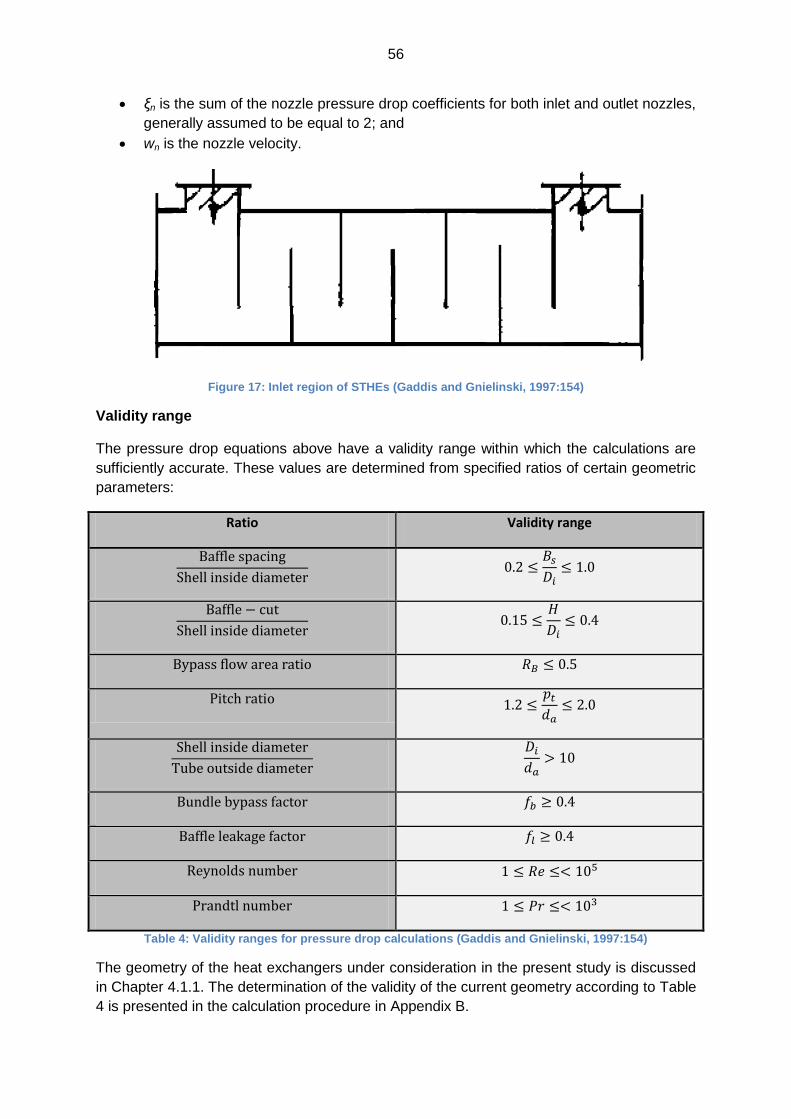
Window zone pressure drop

According to Bell (cited by Gaddis and Gnielinski, 1997:154), the pressure drop in a window

section (Figure 16) for laminar and turbulent flow can be calculated from:

[

⁄

⁄

]

(3.90)

( )

(3.91)

where:

55

e is the minimum distance between tube surfaces;

wz is the characteristic velocity;

μ is the dynamic viscosity;

Nw is the number of major restrictions (tube rows) in the window section;

dg is the hydraulic diameter in the window section; and

Bs is the baffle spacing.

Figure 16: Baffle window region of STHEs (Gaddis and Gnielinski, 1997:154)

The equations for pressure drop in a window section for laminar and turbulent flows give

different values at a Reynolds number equal to 100. Taborek gives the suggestion in the

Heat exchanger design handbook no. 3 (Bell et al., 1983a) that an intermediate value can be

taken, based on a factor of safety and engineering judgment. On the other hand, Gaddis and

Gnielinski propose a method of superposition:

√

(3.92)

(3.93)

(3.94)

with:

the viscosity correction factor;

a viscosity correction factor for laminar flow; and

a viscosity correction factor for turbulent flow.

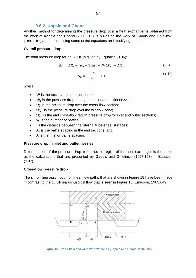
Pressure drop in inlet and outlet nozzles

The reduction in pressure that is experienced in inlet and outlet regions is due to sudden

expansion and contraction (Figure 17). This is calculated as:

(3.95)

where:

56

ξn is the sum of the nozzle pressure drop coefficients for both inlet and outlet nozzles,

generally assumed to be equal to 2; and

wn is the nozzle velocity.

Figure 17: Inlet region of STHEs (Gaddis and Gnielinski, 1997:154)

Validity range

The pressure drop equations above have a validity range within which the calculations are

sufficiently accurate. These values are determined from specified ratios of certain geometric

parameters:

Ratio Validity range

Bypass flow area ratio

Pitch ratio

Bundle bypass factor

Baffle leakage factor

Reynolds number

Prandtl number

Table 4: Validity ranges for pressure drop calculations (Gaddis and Gnielinski, 1997:154)

The geometry of the heat exchangers under consideration in the present study is discussed

in Chapter 4.1.1. The determination of the validity of the current geometry according to Table

4 is presented in the calculation procedure in Appendix B.

57

3.6.2. Kapale and Chand

Another method for determining the pressure drop over a heat exchanger is obtained from

the work of Kapale and Chand (2006:610). It builds on the work of Gaddis and Gnielinski

(1997:157) and others, using some of the equations and modifying others.

Overall pressure drop

The total pressure drop for an STHE is given by Equation (3.96):

( ) (3.96)

(3.97)

where:

is the total overall pressure drop;

is the pressure drop through the inlet and outlet nozzles;

is the pressure drop over the cross-flow section;

is the pressure drop over the window zone;

is the end cross-flow region pressure drop for inlet and outlet sections;

is the number of baffles;

l is the distance between the internal tube-sheet surfaces;

Bse is the baffle spacing in the end sections; and

Bs is the interior baffle spacing.

Pressure drop in inlet and outlet nozzles

Determination of the pressure drop in the nozzle region of the heat exchanger is the same

as the calculations that are presented by Gaddis and Gnielinski (1997:157) in Equation

(3.97).

Cross-flow pressure drop

The simplifying assumption of linear flow paths that are shown in Figure 18 have been made

in contrast to the curvilinear/sinusoidal flow that is seen in Figure 15 (Emerson, 1963:649).

Figure 18: Cross-flow and window-flow zones (Kapale and Chand, 2006:603)

58

Kapale and Chand (2006:603) implemented equations for cross-flow pressure drop,

developed by Bell (cited by Kapale and Chand, 2006:603). The equations were modified to

account for inclined flow, instead of pure cross-flow (GH vs. G1H in Figure 18), as well as

changes in viscosity due to heat transfer:

(

)

(3.98)

where:

f is the friction factor;

usc is the cross-flow velocity;

Nc is the number of cross-flow tube rows (Figure 19);

θ is the flow inclination angle (Figure 18);

μsw is the viscosity of the fluid at wall temperature; and

μs is the viscosity at bulk fluid temperature.

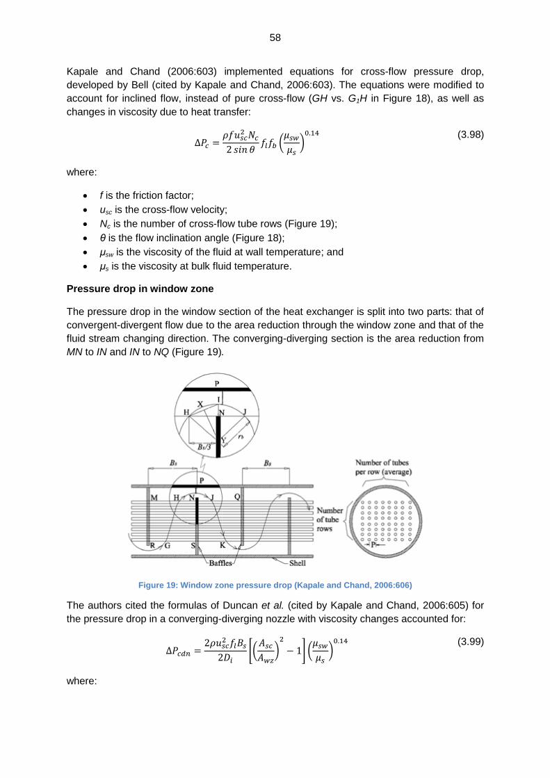
Pressure drop in window zone

The pressure drop in the window section of the heat exchanger is split into two parts: that of

convergent-divergent flow due to the area reduction through the window zone and that of the

fluid stream changing direction. The converging-diverging section is the area reduction from

MN to IN and IN to NQ (Figure 19).

Figure 19: Window zone pressure drop (Kapale and Chand, 2006:606)

The authors cited the formulas of Duncan et al. (cited by Kapale and Chand, 2006:605) for

the pressure drop in a converging-diverging nozzle with viscosity changes accounted for:

[(

)

] (

)

(3.99)

where:

59

is the converging-diverging nozzle pressure drop;

Di is the shell inside diameter;

Asc is the interior cross-flow section at or near the shell centreline; and

Awz is the window zone cross-flow area, excluding the tubes.

The formula for pressure drop due to the streamline curvature of flow in the window zone

was obtained from the work of Ionel (cited by Kapale and Chand, 2006:607):

(3.100)

with:

the pressure drop due to streamline curvature;

uwz the window zone cross-flow velocity; and

kp a pressure drop coefficient.

The total window zone pressure drop is the summation of two constituents: converging-

diverging nozzle and streamline curvature pressure drop:

(3.101)

Pressure drop in end cross-flow region

The authors once again applied the work of Bell (cited by Kapale and Chand, 2006:608), this

time for the calculation of pressure drop in the end cross-flow region. The flow is assumed to

be perpendicular to the tube bundle, with and without the influence of bypass and leakage

streams respectively:

(

) (

)

(3.102)

where:

Nw is the number of tube rows in the window section (Figure 19); and

fs is the end correction factor for unequal baffle spacing.

3.7. Conclusion

In this chapter, the detailed theory behind STHEs and CFD has been described; it is

necessary background information required for insight into the choices of the solution

methodology. The different components have been discussed, along with the advantages

and disadvantages of relevant configuration principles. Definitions and descriptions of the

flow structures that are integral to the designs have also been discussed, highlighting the

importance and influence on the overall effectiveness thereof.

An in-depth discussion on the principles and theory behind CFD has been presented by

deriving and discussing the relevant conservation as well as the realizable k-ε transport

equations. The CFD software’s method of multiphase modelling and treatment of wall-

60

bounded flow has been discussed, broadening the comprehension of the capabilities of

CFD.

Finally, two pressure drop correlations have been discussed concisely, enabling partial

verification of simulation results.

The theoretical breakdown that has been presented facilitates a secure foundation on which

to build a discussion on the setup of the simulation model.