Embed Size (px)
Citation preview

CHAPTER 3 LinearAlgebra
3.1 Matrices: Sums and Products
!!!! Do They Compute?
1. 22 0 64 2 42 0 2
A =−
−
L
NMMM
O
QPPP
2. A B+ =−
L
NMMM
O
QPPP
21 6 32 3 21 0 3
3. 2C D− , Matrices are not compatible
4. AB =− −
− −
L
NMMM
O
QPPP
1 3 32 7 21 3 1
5. BA =−
L
NMMM
O
QPPP
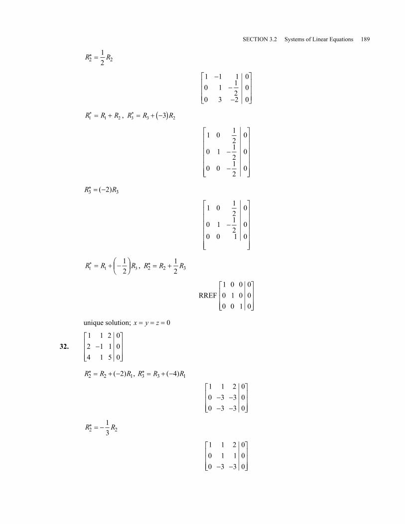
5 3 92 1 21 0 1
6. CD =−−L
NMMM
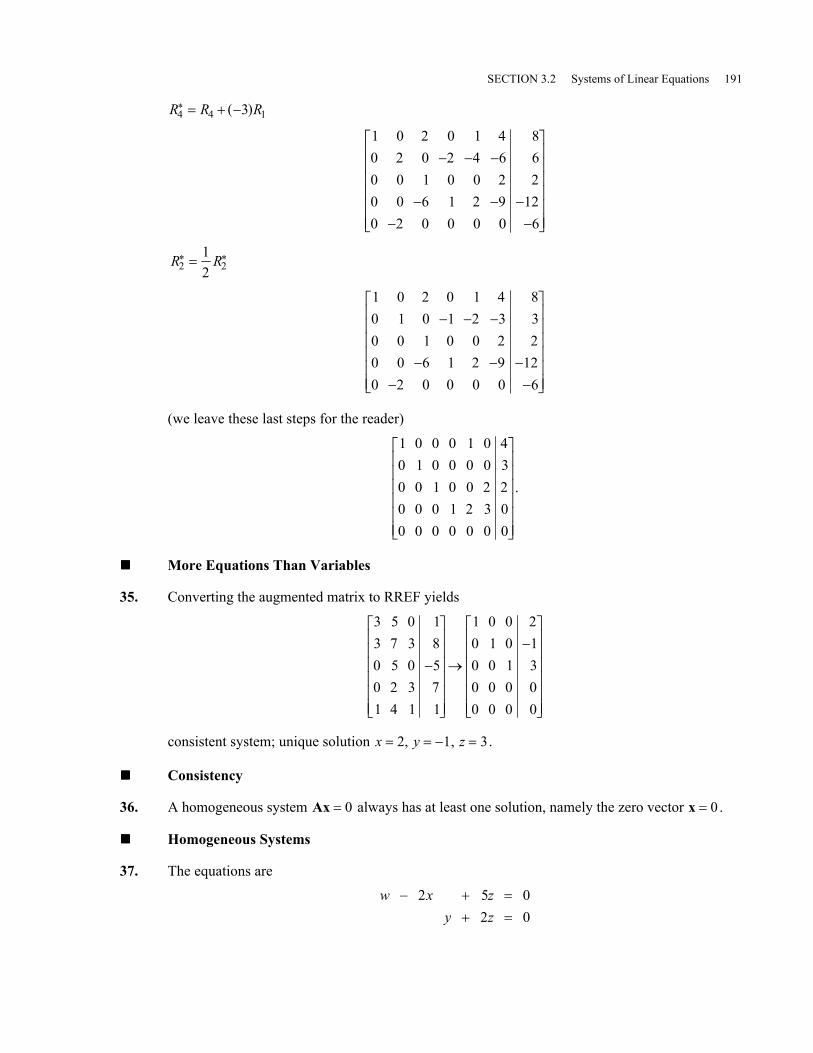
O
QPPP
3 1 08 1 29 2 6
7. DC =−LNMOQP
1 16 7
8. DC( ) =−LNMOQP
T 1 61 7
9. C DT , Matrices are not compatible
10. D CT , Matrices are not compatible
11. A22 0 02 1 100 0 2
=−−
−
L
NMMM
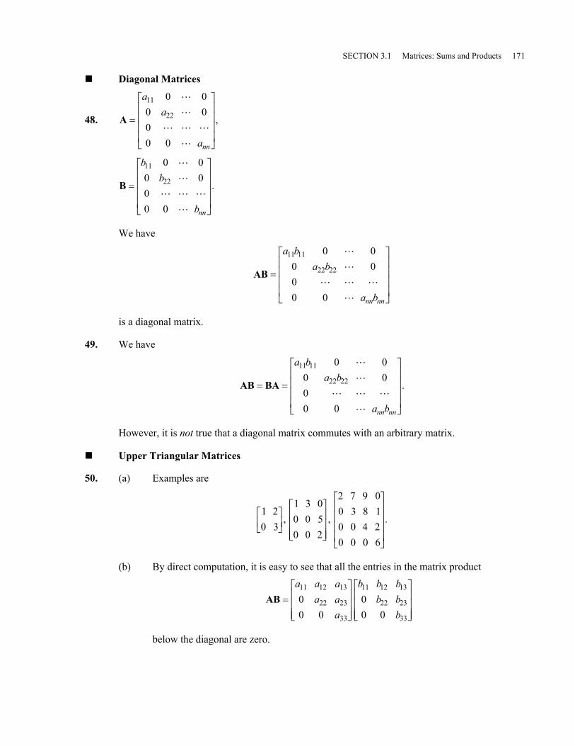
O
QPPP
12. AD, Matrices are not compatible
13. A I− =−
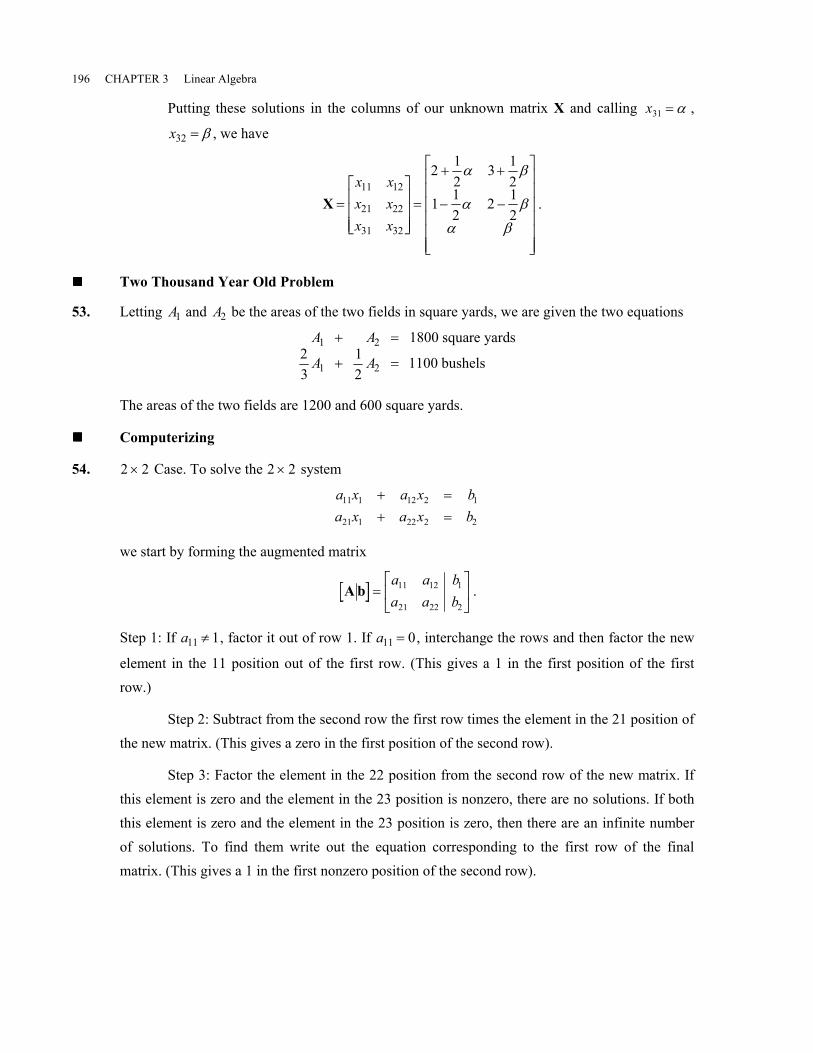
−
L
NMMM
O
QPPP
3
2 0 32 0 21 0 0
14. 4 31 12 00 1 00 0 1
3B I− =L
NMMM
O
QPPP
15. C I− 3, Matrices are not compatible
16. AC =L
NMMM
O
QPPP
2 96 70 3
165
166 CHAPTER 3 Linear Algebra
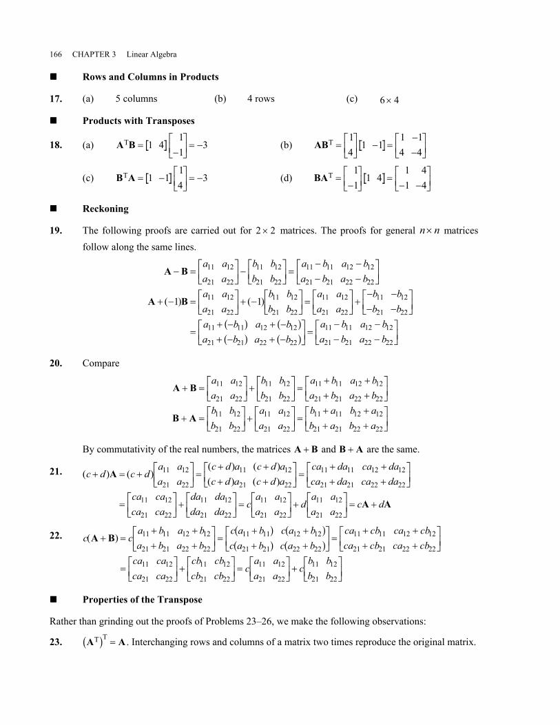
!!!! Rows and Columns in Products
17. (a) 5 columns (b) 4 rows (c) 6 4×
!!!! Products with Transposes
18. (a) A BT =−LNMOQP = −1 4
11
3 (b) ABT = LNMOQP − =
−−LNMOQP
14
1 11 14 4
(c) B AT = − LNMOQP = −1 1
14
3 (d) BAT =−LNMOQP =
− −LNMOQP
11
1 41 41 4
!!!! Reckoning
19. The following proofs are carried out for 2 2× matrices. The proofs for general n n× matricesfollow along the same lines.
A B
A B
− = LNMOQP −LNM
OQP =
− −− −
LNM
OQP
+ −( ) = LNMOQP + −( )LNM
OQP =LNM
OQP +
− −− −LNM
OQP
=+ − + −+ − + −
LNM
OQP =
−
a aa a
b bb b
a b a ba b a b
a aa a
b bb b
a aa a
b bb b
a b a ba b a b
a
11 12
21 22
11 12
21 22
11 11 12 12
21 21 22 22
11 12
21 22
11 12
21 22
11 12
21 22
11 12
21 22
11 11 12 12
21 21 22 22
11
1 1
a f a fa f a f
b a ba b a b
11 12 12
21 21 22 22
−− −
LNM
OQP
20. Compare
A B
B A
+ = LNMOQP +LNM
OQP =
+ ++ +
LNM
OQP
+ = LNMOQP +LNM
OQP =
+ ++ +
LNM
OQP
a aa a
b bb b
a b a ba b a b
b bb b
a aa a
b a b ab a b a
11 12
21 22
11 12
21 22
11 11 12 12
21 21 22 22
11 12
21 22
11 12
21 22
11 11 12 12
21 21 22 22
By commutativity of the real numbers, the matrices A B+ and B A+ are the same.
21. c d c da aa a
c d a c d ac d a c d a
ca da ca daca da ca da
ca caca ca
da dada da
ca aa a
da aa a
c d
+( ) = +( )LNMOQP =
+( ) +( )+( ) +( )LNM
OQP =
+ ++ +
LNM
OQP
= LNMOQP +LNM
OQP =LNM
OQP +LNM
OQP = +
A
A A
11 12
21 22
11 12
21 22
11 11 12 12
21 21 22 22
11 12
21 22
11 12
21 22
11 12
21 22
11 12
21 22
22. c ca b a ba b a b
c a b c a bc a b c a b
ca cb ca cbca cb ca cb
ca caca ca
cb cbcb cb
ca aa a
cb bb b
A B+( ) =+ ++ +
LNM
OQP =
+ ++ +
LNM
OQP =
+ ++ +
LNM
OQP
= LNMOQP +LNM
OQP =LNM
OQP +LNM
OQP
11 11 12 12
21 21 22 22
11 11 12 12
21 21 22 22
11 11 12 12
21 21 22 22
11 12
21 22
11 12
21 22
11 12
21 22
11 12
21 22
a f a fa f a f
!!!! Properties of the Transpose
Rather than grinding out the proofs of Problems 23–26, we make the following observations:
23. A AT Tb g = . Interchanging rows and columns of a matrix two times reproduce the original matrix.
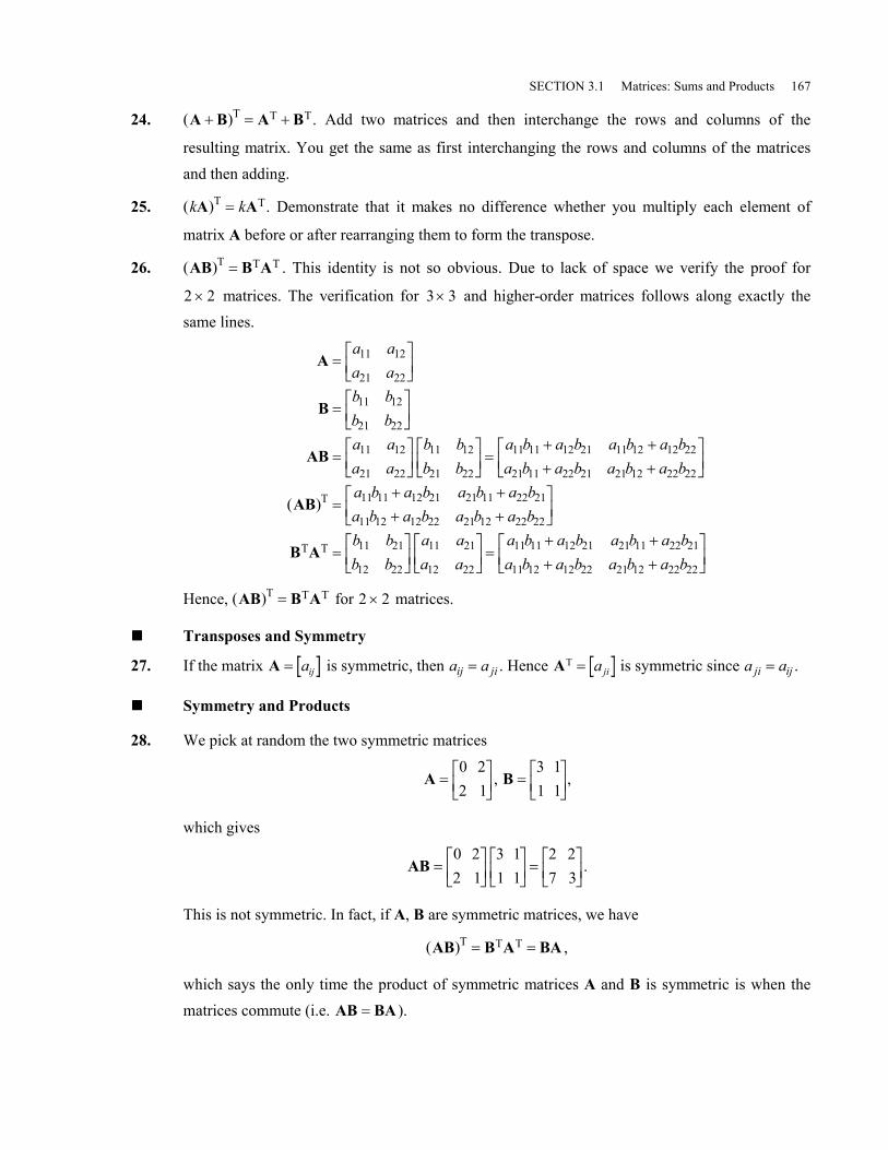
SECTION 3.1 Matrices: Sums and Products 167
24. A B A B+( ) = +T T T. Add two matrices and then interchange the rows and columns of the
resulting matrix. You get the same as first interchanging the rows and columns of the matricesand then adding.
25. k kA A( ) =T T. Demonstrate that it makes no difference whether you multiply each element of
matrix A before or after rearranging them to form the transpose.
26. AB B A( ) =T T T . This identity is not so obvious. Due to lack of space we verify the proof for
2 2× matrices. The verification for 3 3× and higher-order matrices follows along exactly thesame lines.
A
B
AB
AB
B A
= LNMOQP
= LNMOQP
= LNMOQPLNM
OQP =
+ ++ +
LNM
OQP
( ) =+ ++ +
LNM
OQP
= LNMOQP
a aa ab bb ba aa a
b bb b
a b a b a b a ba b a b a b a b
a b a b a b a ba b a b a b a bb bb b
a aa
11 12
21 22
11 12
21 22
11 12
21 22
11 12
21 22
11 11 12 21 11 12 12 22
21 11 22 21 21 12 22 22
11 11 12 21 21 11 22 21
11 12 12 22 21 12 22 22
11 21
12 22
11 21
T
T T
12 22
11 11 12 21 21 11 22 21
11 12 12 22 21 12 22 22aa b a b a b a ba b a b a b a b
LNM
OQP =
+ ++ +
LNM
OQP
Hence, AB B A( ) =T T T for 2 2× matrices.
!!!! Transposes and Symmetry
27. If the matrix A = aij is symmetric, then a aij ji= . Hence AT = aji is symmetric since a aji ij= .
!!!! Symmetry and Products
28. We pick at random the two symmetric matrices
A = LNMOQP
0 22 1
, B = LNMOQP
3 11 1
,
which gives
AB = LNMOQPLNMOQP =LNMOQP
0 22 1
3 11 1
2 27 3
.
This is not symmetric. In fact, if A, B are symmetric matrices, we have
AB B A BA( ) = =T T T ,
which says the only time the product of symmetric matrices A and B is symmetric is when thematrices commute (i.e. AB BA= ).

168 CHAPTER 3 Linear Algebra
!!!! Constructing Symmetry
29. We verify the statement that A A+ T is symmetric for any 2 2× matrix. The general prooffollows along the same lines.
A A+ =LNM
OQP +LNM
OQP =
++
LNM
OQP
T a aa a
a aa a
a a aa a a
11 12
21 22
11 21
12 22
11 12 21
21 12 22
22
,
which is clearly symmetric.
!!!! More Symmetry
30. Let
A =L
NMMM
O
QPPP
a aa aa a
11 12
21 22
31 32
.
Hence, we have
A AT = LNMOQPL
NMMM
O
QPPP= LNM
OQP
a a aa a a
a aa aa a
A AA A
11 21 31
12 22 32
11 12
21 22
31 32
11 12
21 22,
A a a aA a a a a a aA a a a a a a
A a a a
11 112
212
312
12 11 12 21 22 31 32
21 11 12 21 22 31 32
22 122
222
322
= + += + += + +
= + + .
Note A A12 21= , which means AAT is symmetric. We could verify the same result for 3 3×
matrices.
!!!! Trace of a Matrix
31. Tr Tr TrA B A B+ = +b g b g b gTr Tr( ) + Tr(A B+ = + + + + = + + + + + =b g b g b g b g b ga b a b a a b bnn nn nn nn11 11 11 11! ! ! A B) .
32. Tr Trc ca ca c a a cnn nnA A( ) = + + = + + = ( )11 11! !a f33. Tr TrTA Ab g = ( ). Taking the transpose of a (square) matrix does not alter the diagonal element, so
Tr Tr TA A( ) = b g.34. Tr
Tr
AB
BA
( ) = + + ⋅ + + + + + + ⋅ + += + + + + + += + + + + + += + + ⋅ + + + + + + ⋅ + + = ( )
a a b b a a b ba b a b a b a bb a b a b a b ab b a a b b a a
n n n nn n nn
n n n n nn nn
n n n n nn nn
n n n nn n nn
11 1 11 1 1 1
11 11 1 1 1 1
11 11 1 1 1 1
11 1 11 1 1 1
! ! ! ! !! ! !! ! !
! ! ! ! !
a f a fa f a f
!!!! Matrices Can Be Complex
35. A B+ =++ −LNM
OQP2
3 02 4 4
ii i
36. AB =− + − ++ −LNM
OQP
3 18 4 5 3
i ii i
37. BA =− −
−LNM
OQP
1 34 1
ii i
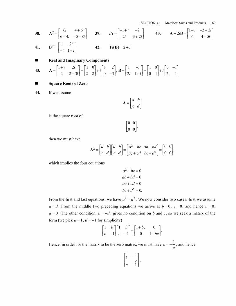
SECTION 3.1 Matrices: Sums and Products 169
38. A2 6 4 66 4 5 8
=+
− − −LNM
OQP
i ii i
39. ii
i iA =
− + −+
LNM
OQP
1 22 3 2
40. A B− =− − +
−LNM
OQP2
1 2 26 4 5
ii i
i
41. BT =− +LNM
OQP
1 21
ii i
42. Tr B( ) = +2 i
!!!! Real and Imaginary Components
43. A =+
−LNM
OQP =LNMOQP + −LNMOQP
1 22 2 3
1 02 2
1 20 3
i ii
i , B =−+
LNM
OQP =LNMOQP +
−LNMOQP
12 1
1 00 1
0 12 1
ii i
i
!!!! Square Roots of Zero
44. If we assume
A = LNMOQP
a bc d
is the square root of
0 00 0LNMOQP ,
then we must have
A22
2
0 00 0
= LNMOQPLNMOQP =
+ ++ +LNM
OQP =LNMOQP
a bc d
a bc d
a bc ab bdac cd bc d
,
which implies the four equations
a bcab bdac cdbc d
2
2
0000
+ =+ =+ =
+ = .
From the first and last equations, we have a d2 2= . We now consider two cases: first we assumea d= . From the middle two preceding equations we arrive at b = 0, c = 0, and hence a = 0,d = 0 . The other condition, a d= − , gives no condition on b and c, so we seek a matrix of theform (we pick a = 1, d = −1 for simplicity)
11
11
1 00 1
bc
bc
bcbc−
LNMOQP −LNMOQP =
++
LNM
OQP .
Hence, in order for the matrix to be the zero matrix, we must have bc
= −1 , and hence
1 1
1−
−
LNMMOQPPcc
,

170 CHAPTER 3 Linear Algebra
which gives
1 1
11 1
1
0 00 0
−
−
LNMMOQPP
−
−
LNMMOQPP =LNMOQPc
cc
c.
!!!! Zero Divisors
45. No, AB = 0 does not imply that A = 0 or B = 0 . For example, the product
1 00 0
0 00 1
LNMOQPLNMOQP
is the zero matrix, but neither factor is itself the zero matrix.
!!!! Does Cancellation Work?
46. No. A counter example is: 0 00 1
1 20 4
0 00 1
0 00 4
FHGIKJFHGIKJ =FHGIKJFHGIKJ since
1 20 4
0 00 4
FHGIKJ ≠FHGIKJ .
!!!! Taking Matrices Apart
47. (a) A A A A= = −L
NMMM
O
QPPP
1 2 3
1 5 21 0 32 4 7
, x =L
NMMM
O
QPPP
243
where A1, A2 , and A3 are the three columns of the matrix A and x1 2= , x2 4= , x3 3=
are the elements of x. We can write
A
A A A
x
x x x
= −L
NMMM
O
QPPP
L
NMMM
O
QPPP=
× + × + ×− × + × + ×× + × + ×
L
NMMM
O
QPPP= −L
NMMM
O
QPPP+L
NMMM
O
QPPP+L
NMMM
O
QPPP
= + +
1 5 21 0 32 4 7
243
1 2 5 4 2 31 2 0 4 3 32 2 4 4 7 3
2112
4504
3237
1 1 2 2 3 3 .
(b) We verify the fact for a 3 3× matrix. The general n n× case follows along the samelines.
Axa a aa a aa a a
xxx
a x a x a xa x a x a xa x a x a x
a xa xa x
a xa xa x
a xa xa x
xaaa
=L
NMMM
O
QPPP
L
NMMM
O
QPPP=
+ ++ ++ +
L
NMMM
O
QPPP=L
NMMM
O
QPPP+L
NMMM
O
QPPP+L
NMMM
O
QPPP
=L
11 12 13
21 22 23
31 32 33
1
2
3
11 1 12 2 13 3
21 1 22 2 23 3
31 1 32 2 33 3
11 1
21 1
31 1
12 2
22 2
32 2
13 3
23 3
33 3
1
11
21
31NMMM
O
QPPP+L
NMMM
O
QPPP+L
NMMM
O
QPPP= + +x
aaa
xaaa
x x x2
12
22
32
3
13
23
33
1 1 2 2 3 3A A A
SECTION 3.1 Matrices: Sums and Products 171
!!!! Diagonal Matrices
48. A =
L
N
MMMM
O
Q
PPPP
aa
ann
11
22
0 00 000 0
!!
! ! !!
,
B =
L
N
MMMM
O
Q
PPPP
bb
bnn
11
22
0 00 000 0
!!
! ! !!
.
We have
AB =
L
N
MMMM
O
Q
PPPP
a ba b
a bnn nn
11 11
22 22
0 00 000 0
!!
! ! !!
is a diagonal matrix.
49. We have
AB BA= =
L
N
MMMM
O
Q
PPPP
a ba b
a bnn nn
11 11
22 22
0 00 000 0
!!
! ! !!
.
However, it is not true that a diagonal matrix commutes with an arbitrary matrix.
!!!! Upper Triangular Matrices
50. (a) Examples are
1 20 3LNMOQP ,
1 3 00 0 50 0 2
L
NMMM
O
QPPP
,
2 7 9 00 3 8 10 0 4 20 0 0 6
L
N
MMMM
O
Q
PPPP.
(b) By direct computation, it is easy to see that all the entries in the matrix product
AB =L
NMMM
O
QPPP
L
NMMM
O
QPPP
a a aa a
a
b b bb b
b
11 12 13
22 23
33
11 12 13
22 23
33
00 0
00 0
below the diagonal are zero.

172 CHAPTER 3 Linear Algebra
(c) In the general case, if we multiply two upper-triangular matrices, it yields
AB =
L
N
MMMMMM
O
Q
PPPPPP
×
L
N
MMMMMM
O
Q
PPPPPP
=
L
N
MMMMMM
O
Q
PPPPPP
a a a aa a a
a a
a
b b b bb b b
b b
b
c c c cc c c
c c
c
n
n
n
nn
n
n
n
nn
n
n
n
nn
11 12 13 1
22 23 2
33 3
11 12 13 1
22 23 2
33 3
11 12 13 1
22 23 2
33 3
00 0
0 0 0 0
00 0
0 0 0 0
00 0
0 0 0 0
!!!
! ! ! ! !
!!!
! ! ! ! !
!!!
! ! ! ! !.
We won’t bother to write the general expression for the elements cij ; the important point
is that the entries in the product matrix that lie below the main diagonal are clearly zero.
!!!! Hard Puzzle
51. If
M = LNMOQP
a bc d
is a square root of
A = LNMOQP
0 10 0
,
then
M2 0 10 0
= LNMOQP ,
which leads to the condition a d2 2= . Each of the possible cases leads to a contradiction. How-ever for matrix B because
1 01
1 01
1 00 1α α−
LNMOQP −LNMOQP =LNMOQP
for any α, we conclude that
B =−
LNMOQP
1 01α
is a square root of the identity matrix for any number α.
!!!! Dot Products
52. 2, 1 1 2 0 • − =, , orthogonal
53. − • = −3 0 2, 1 6, , not orthogonal. Because the dot product is negative, this means the angle
between the vectors is greater than 90°.
54. 2, 1 2 3 1 0 5 , , ,• − = . Because the dot product is positive, this means the angle between the
vectors is less than 90°.
SECTION 3.1 Matrices: Sums and Products 173
55. 1 0 1 1 1 1 0, , , , − • = , orthogonal
56. 5 7, 1 2, 4, 3 3 0, , , 5 • − − − = , orthogonal
57. 7, 1 4, 3 2, 3 30 5 5 , , ,• − = , not orthogonal
!!!! Lengths
58. Introducing the two vectors u = a b, , v = c d, , we have the distance d between the heads of
the vectors
d a c b d= −( ) + −( )2 2 .
But we also have
u v u v u v− = −( ) ⋅ −( ) = −( ) + −( )2 2 2a c b d ,
so d = −u v . This proof can be extended easily to "u and "v in Rn .
!!!! Geometric Vector Operations
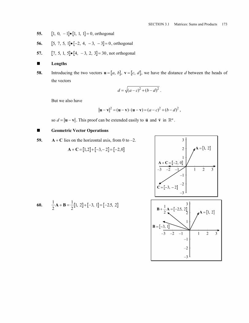
59. A C+ lies on the horizontal axis, from 0 to –2.
A C+ = + − − = −1 2 3 2 2,0, ,
1 3–1–1
–2
–3
1
3
2
–2
–3 2
A = 1 2,
C = − −3 2,
A C+ = −2, 0
60. 12
12
1 2 3 1 2 5 2A B+ = + − = −, , . ,
1 3–1–1
–2
–3
1
3
2
–2
–3 2
A = 1 2,B A+ = −
12
25 2. ,
B = −3 1,
174 CHAPTER 3 Linear Algebra
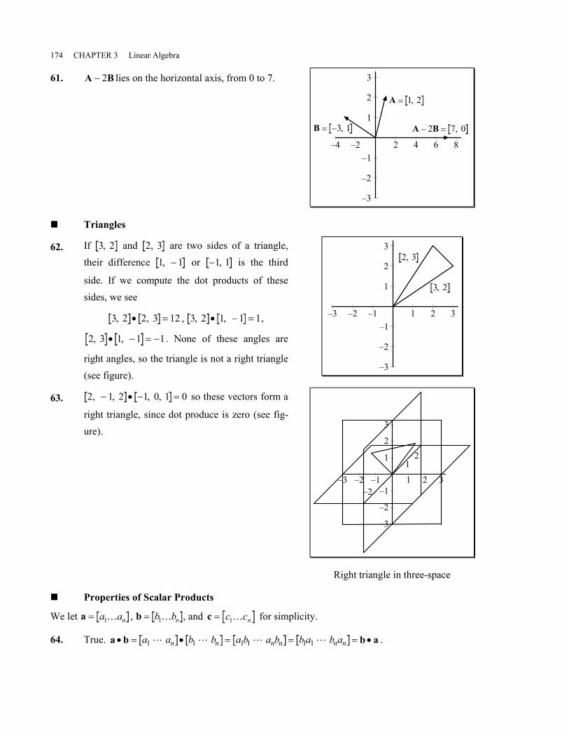
61. A B− 2 lies on the horizontal axis, from 0 to 7.
4 82–1
–2
–3
1
3
2
–2
–4 6
A = 1 2,
B = −3 1, A B− =2 7, 0
!!!! Triangles
62. If 3 2, and 2, 3 are two sides of a triangle,their difference 1 1, − or −1 1, is the third
side. If we compute the dot products of thesesides, we see
3 2 2, 3 12, • = , 3 2 1 1 1, , • − = ,
2 1 1 1, , 3 • − = − . None of these angles are
right angles, so the triangle is not a right triangle(see figure).
1 3–1–1
–2
–3
1
3
2
–2
–3 2
2, 3
3 2,
63. 2, 1 2 1 0 1 0 − • − =, , , so these vectors form a
right triangle, since dot produce is zero (see fig-ure).
1 3–1–1
–2
–3
1
3
2
–2
–3 2
12
–2
Right triangle in three-space
!!!! Properties of Scalar Products
We let a = a an1… , b = b bn1… , and c = c cn1… for simplicity.
64. True. a b b a• = • = = = •a a b b a b a b b a b an n n n n n1 1 1 1 1 1 ! ! ! ! .

SECTION 3.1 Matrices: Sums and Products 175
65. False. Neither a b c• •( ) nor a b c•( )• . Invalid operation, since we ask for the scalar product of a
vector and a scalar.
66. True.
k ka ka b b ka b ka b a kb a kb
a a kb kb kn n n n n n
n n
a b
a bb g
b g• = • = + + = + +
= • = •1 1 1 1 1 1
1 1
! ! ! !
! !
67. True.
a b c
a b a c
• + = • + + = + + + +
= + + + + + = • + •
b g b g b gb g b ga a b c b c a b c a b c
a b a b a c a cn n n n n n
n n n n
1 1 1 1 1 1
1 1 1 1
! ! !
! !
!!!! Markov Chains
68.1 00 1LNMOQP . Markov chain.
Yes; with square matrix with entries between 0 and 1 inclusive,column sums are 1. We draw the Markov tree for two stagesstarting in state 1. 2
11
1
2
2
1
1
0
1
0
0
1
69.05 0505 05. .. .LNMOQP . Markov chain.
Yes; with square matrix with entries between 0 and 1 inclusive,column sums are 1. We draw the Markov tree for two stagesstarting in state 1. 2
11
1
2
2
1
0.5
0.5
0.5
0.5
0.5
0.5
70.0 051 05
.
.LNMOQP . Markov chain.
Yes; with square matrix with entries between 0 and 1 inclusive,column sums are 1. We draw the Markov tree for two stagesstarting in state 1. 2
11
1
2
2
1
0
1
0
1
0.5
0.5
71.0 11 0LNMOQP . Markov chain.
Yes; with square matrix with entries between 0 and 1 inclusive,column sums are 1. We draw the Markov tree for two stagesstarting in state 1. Note that the states on this Markov chainalternate from state 1 to state 2.
2
1
1
1
2
0
1 1
0
176 CHAPTER 3 Linear Algebra
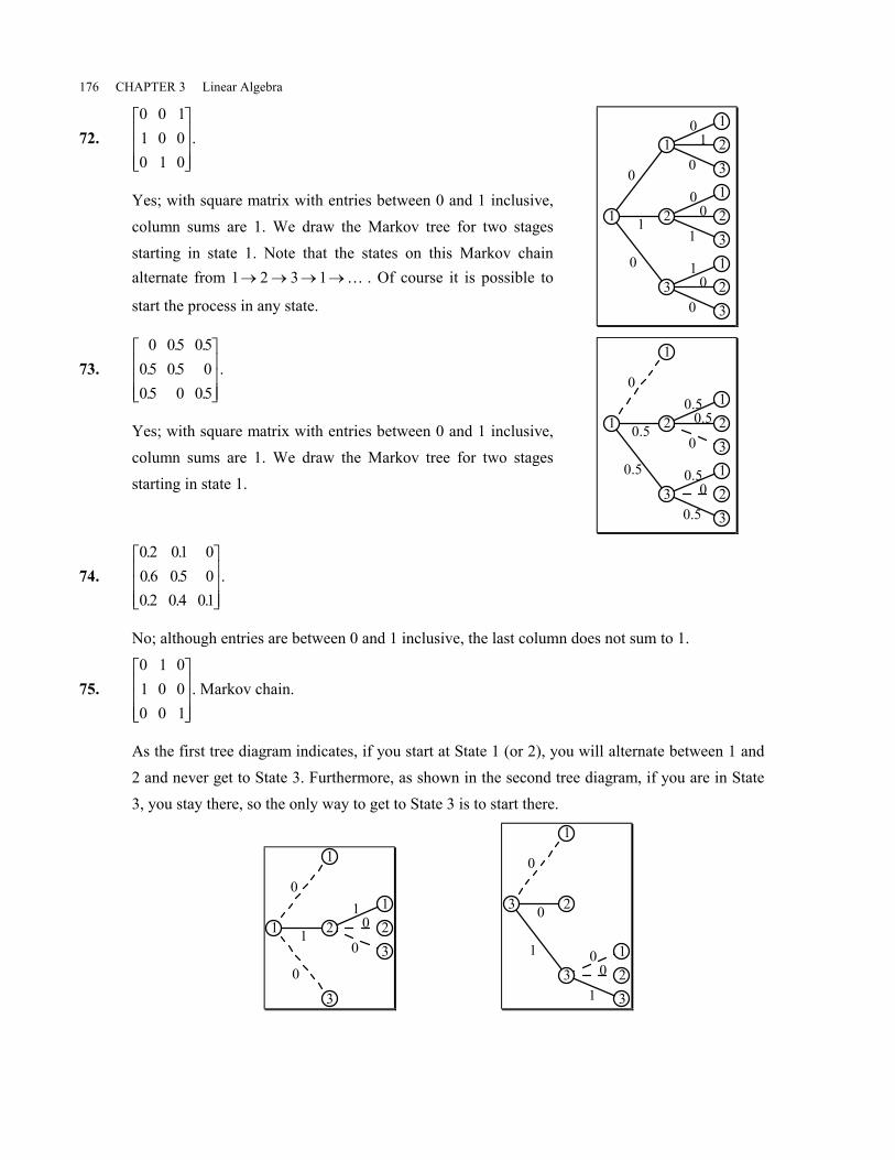
72.0 0 11 0 00 1 0
L
NMMM
O
QPPP.
Yes; with square matrix with entries between 0 and 1 inclusive,column sums are 1. We draw the Markov tree for two stagesstarting in state 1. Note that the states on this Markov chainalternate from 1 2 3 1→ → → →… . Of course it is possible to
start the process in any state.
1
13
10
021
23
10
120
33
11
020
0
0
1
73.0 05 05
05 05 005 0 05
. .. .. .
L
NMMM
O
QPPP
.
Yes; with square matrix with entries between 0 and 1 inclusive,column sums are 1. We draw the Markov tree for two stagesstarting in state 1.
1
1
23
10.5
020.5
33
10.5
0.520
0
0.5
0.5
74.0 2 01 00 6 05 00 2 0 4 01
. .
. .
. . .
L
NMMM
O
QPPP.
No; although entries are between 0 and 1 inclusive, the last column does not sum to 1.
75.0 1 01 0 00 0 1
L
NMMM
O
QPPP. Markov chain.
As the first tree diagram indicates, if you start at State 1 (or 2), you will alternate between 1 and2 and never get to State 3. Furthermore, as shown in the second tree diagram, if you are in State3, you stay there, so the only way to get to State 3 is to start there.
1
1
23
11
020
3
0
0
1
3
1
2
3
10
1203
0
1
0

SECTION 3.1 Matrices: Sums and Products 177
!!!! Best-of-Three-Game Series
76. (a) (from this state)2 0 2 1 1 0 1 1 0 0 0 1 1 2 0 2
1 0.61 0.6
0.60.4 0.6
0.40.4 1
0.4 1
2 02 11 01 10 00 11 20 2
- - - - - - - ---------
0 0 0 0 0 00 0 0 0 0 00 0 0 0 0 0 00 0 0 0 0 00 0 0 0 0 0 0 00 0 0 0 0 0 00 0 0 0 0 00 0 0 0 0 0
L
N
MMMMMMMMMM
O
Q
PPPPPPPPPP
(b) The Bulls will win the series in one of three ways: if they win the first two (WW); losethe first and win the next two (LWW); or win the first, lose the second and win the third(WLW). Because the probabilities of these disjoint events is
P WW
P LWW
P WLW
( ) = ( )
( ) = ( )( )
( ) = ( ) ( )
06
04 04
06 0 4
2
2
2
.
. .
. .
we haveP Bulls win the series P WW P LWW WLW( ) = ( ) + ( ) + ( )
= ( ) + ( )( ) + ( ) ( ) =06 0 4 06 06 04 06482 2 2. . . . . .
Hence, the probability the Knicks will win the three-game series is 0.352.
!!!! Flipping Coins
77. We designate the state of the system as the number of dollars that Jerry has in his pocket. This isan absorbing random walk problem. Once Jerry reaches state $0 or $5 the game is over.
For each player there are six states: $0, $1, $2, $3, $4, $5. From Jerry’s point of view,
x0
000100
=
L
N
MMMMMMMM
O
Q
PPPPPPPP
, P =
L
N
MMMMMMMM
O
Q
PPPPPPPP
1 0 5 0 0 0 00 0 0 5 0 0 00 0 5 0 0 5 0 00 0 0 5 0 0 5 00 0 0 0 5 0 00 0 0 0 0 5 1
..
. .. .
..
P x50 tells us that there is a 22% chance Jerry will be broke after 5 tosses and a 38% chance he
will win everything from Sheryl.

178 CHAPTER 3 Linear Algebra
!!!! Genetics Problem
78. If we square the transition matrix
Red Pink White NextRedPinkWhite
P =L
NMMM
O
QPPP
0 5 0 25 00 5 0 5 0 50 0 25 0 5
. .
. . .. .
we get
P2
0 375 0 25 01250 5 0 5 0 50125 0 25 0 375
=L
NMMM
O
QPPP
. . .
. . .
. . ..
This tells us two things: the Markov chain is regular and that if the initial mixture of roses is theproportion 0 5 0 5 0. : . : , then the next generation should expect to be
0 375 0 25 012505 05 050125 0 250 0 375
0 50 50
031250 5001875
. . .
. . .
. . .
.
....
L
NMMM
O
QPPP
L
NMMM
O
QPPP=L
NMMM
O
QPPP.
To find the limiting ratio of genotypes, instead of solving the usual system of equations, we cancompute powers of P until there is no change. We find
P P5 6025 025 0 25050 050 050025 025 0 25
= =L
NMMM
O
QPPP
. . .
. . .
. . ..
This tells us the powers of the transition matrix have stabilized to a matrix. When this happensthe steady state probability vector s is the common column of this matrix. In this case it iss = 025 050 025. , . , . . In other words, after a few generations, the ratios of the three genotypeswill be 0 25 0 50 0 25. : . : . .
!!!! Estimating a Transition Matrix
79. Among the 19 ones in the sequence there are 6 that are followed by ones and 13 followed by
twos so the probability of moving from one to one is 619
032≈ . , and the probability of moving to
State 2, given we are in State 1, is 1319
068≈ . . On the other hand, among the 20 twos (we don’t
count the very last 2), 12 are followed by a one and eight are followed by a two. Hence, we
would say that the probability of moving to State 1, given we are in State 2, is 1220
060= . , and the
SECTION 3.1 Matrices: Sums and Products 179
probability of moving to State 2, given we are in State 2, is 820
040= . . Hence, we have the
transition matrix1 2
12
P = LNMOQP
0 32 0 600 68 0 40. .. .
.
!!!! Directed Graphs
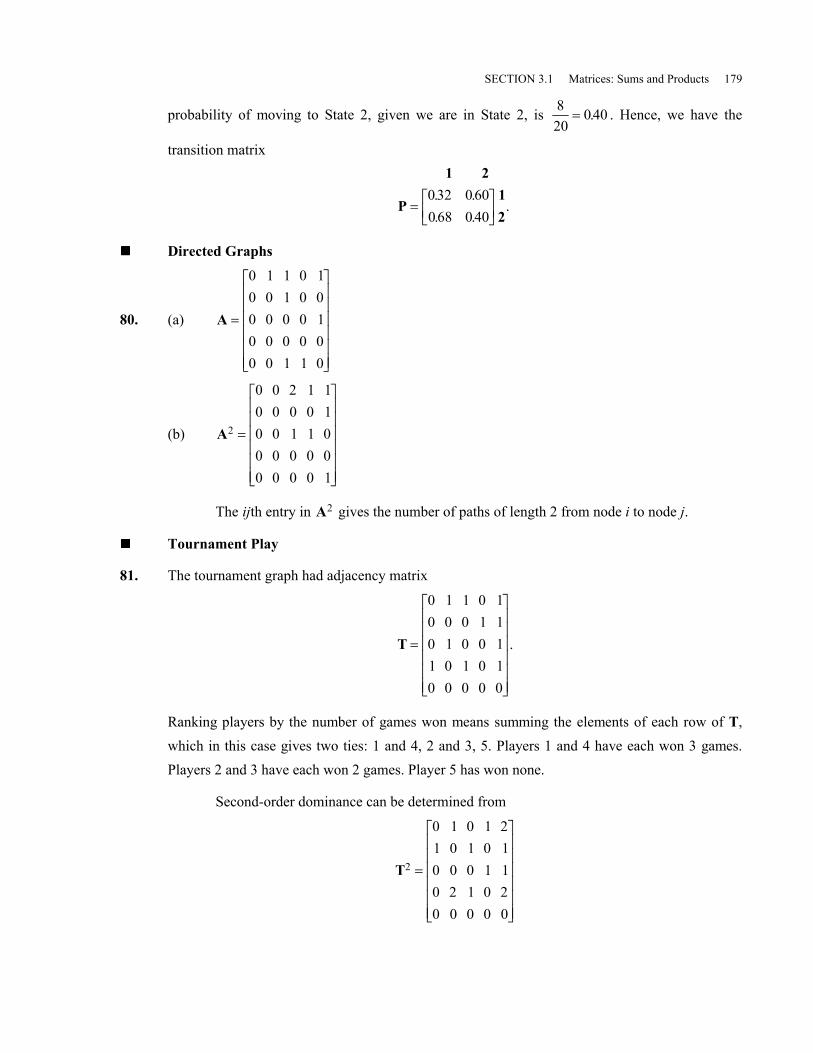
80. (a) A =
L
N
MMMMMM
O
Q
PPPPPP
0 1 1 0 10 0 1 0 00 0 0 0 10 0 0 0 00 0 1 1 0
(b) A2
0 0 2 1 10 0 0 0 10 0 1 1 00 0 0 0 00 0 0 0 1
=
L
N
MMMMMM
O
Q
PPPPPPThe ijth entry in A2 gives the number of paths of length 2 from node i to node j.
!!!! Tournament Play
81. The tournament graph had adjacency matrix
T =
L
N
MMMMMM
O
Q
PPPPPP
0 1 1 0 10 0 0 1 10 1 0 0 11 0 1 0 10 0 0 0 0
.
Ranking players by the number of games won means summing the elements of each row of T,which in this case gives two ties: 1 and 4, 2 and 3, 5. Players 1 and 4 have each won 3 games.Players 2 and 3 have each won 2 games. Player 5 has won none.
Second-order dominance can be determined from
T2
0 1 0 1 21 0 1 0 10 0 0 1 10 2 1 0 20 0 0 0 0
=
L
N
MMMMMM
O
Q
PPPPPP

180 CHAPTER 3 Linear Algebra
For example, T2 tells us that Player 1 can dominate Player 5 in two second-order ways (bybeating either Player 2 or Player 4, both of whom beat Player 5). The sum
T T+ =
L
N
MMMMMM
O
Q
PPPPPP
2
0 2 1 1 31 0 1 1 20 1 0 1 21 2 2 0 30 0 0 0 0
,
gives the number of ways one player has beaten another both directly and indirectly. Rerankingplayers by sums of row elements of T T+ 2 can sometimes break a tie: In this case it does so andranks the players in order 4, 1, 2, 3, 5.
!!!! Suggested Journal Entry
82. Student Project

SECTION 3.2 Systems of Linear Equations 181
3.2 Systems of Linear Equations
!!!! Matrix-Vector Form
1.1 22 13 2
101
−L
NMMM
O
QPPPLNMOQP =L
NMMM
O
QPPP
xy
2.1 2 1 31 3 3 0
21
1
2
3
4
−LNM
OQPL
N
MMMM
O
Q
PPPP= LNMOQP
iiii
Augmented matrix = −L
NMMM
O
QPPP
1 2 12 1 03 2 1
Augmented matrix =−LNM
OQP
1 2 1 3 21 3 3 0 1
3.1 2 11 3 30 4 5
113
−−
L
NMMM
O
QPPP
L
NMMM
O
QPPP=L
NMMM
O
QPPP
rst
4. 1 2 3 01
2
3
−L
NMMM
O
QPPP=
xxx
Augmented matrix = −−
L
NMMM
O
QPPP
1 2 1 11 3 3 10 4 5 3
Augmented matrix = −1 2 3 0|
!!!! Solutions in R2
5. (A) 6. (B) 7. (C) 8. (B) 9. (A)
!!!! A Special Solution Set in R3
10. The three equationsx y zx y zx y z
+ + =+ + =+ + =
12 2 2 23 3 3 3
are equivalent to the single plane x y z+ + = 1, which can be written in parametric form by lettingy s= , z t= . We then have the parametric form 1− −( )s t s t s t, , : , any real numbersk p .
!!!! Reduced Row Echelon Form
11. RREF 12. Not RREF (not all zeros above leading ones)
13. Not RREF (leading nonzero element in row 2 is not 1; not all zeros above the leading ones)
14. Not RREF (row 3 does not have a leading one, nor does it move to the right; plus pivot columnshave nonzero entries other than the leading ones)
15. RREF 16. Not RREF (not all zeros above leading ones)

182 CHAPTER 3 Linear Algebra
17. Not RREF (not all zeros above leading ones)
18. RREF 19. RREF
!!!! Gauss-Jordan Elimination
20. RREF. Starting with1 3 8 00 1 2 10 1 2 4
L
NMMM
O
QPPP
R R R3 3 21∗ = + −( )
1 3 8 00 1 2 10 0 0 3
L
NMMM
O
QPPP
R R3 313
∗ =
1 3 8 00 1 2 10 0 0 1
L
NMMM
O
QPPP.
This matrix is in row echelon form. To further reduce it to RREF we carry out the followingelementary row operations
R R R1 1 23∗ = + −( ) , R R R2 2 31∗ = + −( )
1 0 2 00 1 2 00 0 0 1
L
NMMM
O
QPPP← RREF.
Hence, we see the leading ones in this RREF form are in columns 1, 2, and 4, so the pivotcolumns of the original matrix are columns 1, 2, and 4 shown in bold and underlined as follows:
1 3 00 1 10 1 4
822
L
NMMM
O
QPPP.
21.0 0 2 2 22 2 6 14 4
−LNM
OQP
R R1 2↔
2 2 6 14 40 0 2 2 2−LNM
OQP
SECTION 3.2 Systems of Linear Equations 183
R R1 112
∗ =
1 1 3 7 20 0 2 2 2−LNM
OQP
R R2 212
∗ =
1 1 3 7 20 0 1 1 1−LNM
OQP .
The matrix is in row echelon form. To further reduce it to RREF we carry out the followingelementary row operation.
R R R1 1 23∗ = + −( )
1 1 0 4 50 0 1 1 1−LNM
OQP← RREF
pivot columns of the original matrix are first and third.
0 22 6
0 2 22 14 4
−LNM
OQP.
22.
1 0 02 4 65 8 120 8 12
L
N
MMMM
O
Q
PPPP
R R R2 2 12∗ = + −( ) , R R R3 3 15∗ = + −( )
1 0 00 4 60 8 120 8 12
L
N
MMMM
O
Q
PPPP
R R2 214
∗ =
1 0 00 1 3
20 8 120 8 12
L
N
MMMM
O
Q
PPPP

184 CHAPTER 3 Linear Algebra
R R R3 3 28∗ = + −( ) , R R R4 4 28∗ = + −( )
1 0 00 1 3
20 0 00 0 0
L
N
MMMM
O
Q
PPPP← RREF .
This matrix is in both row echelon form and RREF form.
1 02 45 80 8
06
1212
L
N
MMMM
O
Q
PPPP
pivot columns of the original matrix are first and second.
23.1 2 3 13 7 10 42 4 6 2
L
NMMM
O
QPPP
R R R2 2 13∗ = + −( ) , R R R3 3 12∗ = + −( )
1 2 3 10 1 1 10 0 0 0
L
NMMM
O
QPPP← row echelon form.
The matrix is in row echelon form. To further reduce it to RREF, we carry out the followingelementary row operation.
R R R1 1 22∗ = + −( )
1 0 1 10 1 1 10 0 0 0
−L
NMMM
O
QPPP← RREF
pivot columns of the original matrix are first and second.1 23 72 4
3 110 46 2
L
NMMM
O
QPPP
.

SECTION 3.2 Systems of Linear Equations 185
!!!! Solving Systems
24.1 1 41 1 0−LNM
OQP
R R R2 2 11∗ = + −( )
1 1 40 2 4− −LNM
OQP
R R2 212
* = −
1 1 40 1 2LNMOQP
R R R1 1 21∗ = + −b g1 0 20 1 2LNM
OQP
x = 2, y = 2 (unique solution)
25.2 1 01 1 3−− −LNM
OQP
R R1 2↔
1 1 32 1 0
− −−LNM
OQP
R R R2 2 12∗ = + −( )
1 1 30 1 6
− −LNM
OQP
R R R1 1 21∗ = + b g
RREF 1 0 30 1 6LNMOQP
unique solution; x = 3, y = 6
26.1 1 1 00 1 1 1LNM
OQP
R R R1 1 21∗ = + −( )
RREF 1 0 0 10 1 1 1
−LNM
OQP
arbitrary (infinitely many solutions); x = −1, y z= −1
186 CHAPTER 3 Linear Algebra
27.2 4 2 05 3 0 0
−LNM
OQP
R R1 112
∗ =
1 2 1 05 3 0 0
−LNM
OQP
R R R2 2 15∗ = + −( )
1 2 1 00 7 5 0
−−LNM
OQP
R R2 217
∗ = −
1 2 1 00 1 5
70
−−
LNMM
OQPP
R R R1 1 22∗ = + −( )
RREF 1 0 3
70
0 1 57
0−
L
NMMM
O
QPPP
nonunique solutions; x z= −37
, y z=57
, z is arbitrary
28.1 1 2 12 3 1 25 4 2 4
− −L
NMMM
O
QPPP
R R R2 2 12∗ = + −( ) , R R R3 3 15∗ = + −( )
1 1 2 10 5 5 00 9 12 1
− −
−
L
NMMM
O
QPPP
R R2 215
∗ =
1 1 2 10 1 1 00 9 12 1
− −
−
L
NMMM
O
QPPP
SECTION 3.2 Systems of Linear Equations 187
R R R1 1 2∗ = + , R R R3 3 29∗ = + −b g
1 0 1 10 1 1 00 0 3 1
−
−
L
NMMM
O
QPPP
R R3 313
∗ =
1 0 1 10 1 1 00 0 1 1
3
−
−
L
N
MMMM
O
Q
PPPPR R R1 1 3∗ = + , R R R2 2 31∗ = + −b g
RREF
1 0 0 23
0 1 0 13
0 0 1 13
−
L
N
MMMMMM
O
Q
PPPPPP
x = 23
, y = 13
, z = − 13
unique solution
29.1 4 5 02 1 8 9
−−LNM
OQP
R R R2 2 12∗ = + −( )
1 4 5 00 9 18 9
−−LNM
OQP
R R2 219
∗ = −
1 4 5 00 1 2 1
−− −
LNM
OQP
R R R1 1 24∗ = + −( )
RREF 1 0 3 40 1 2 1− −LNM
OQP
nonunique solutions; x x1 34 3= − , x x2 31 2= − + , x3 is arbitrary

188 CHAPTER 3 Linear Algebra
30.1 0 1 22 3 5 43 2 1 4−
−
L
NMMM
O
QPPP
R R R2 2 12∗ = + −( ) , R R R3 3 13∗ = + −( )
1 0 1 20 3 3 00 2 4 2−
− −
L
NMMM
O
QPPP
R R2 213
∗ = −
1 0 1 20 1 1 00 2 4 2
−− −
L
NMMM
O
QPPP
R R R3 3 22∗ = + −( )
1 0 1 20 1 1 00 0 2 2
−− −
L
NMMM
O
QPPP
R R3 312
∗ = −
1 0 1 20 1 1 00 0 1 1
−L
NMMM
O
QPPP
R R R1 1 31∗ = + −( ) , R R R2 2 3∗ = +
RREF 1 0 0 10 1 0 10 0 1 1
L
NMMM
O
QPPP
unique solution;x y z= = = 1
31.1 1 1 01 1 0 01 2 1 0
−
−
L
NMMM
O
QPPP
R R R2 2 11∗ = + −( ) , R R R3 3 11∗ = + −( )
1 1 1 00 2 1 00 3 2 0
−−−
L
NMMM
O
QPPP
SECTION 3.2 Systems of Linear Equations 189
R R2 212
∗ =
1 1 1 00 1 1
20
0 3 2 0
−−
−
L
NMMM
O
QPPP
R R R1 1 2∗ = + , R R R3 3 23∗ = + −b g
1 0 12
0
0 1 12
0
0 0 12
0
−
−
L
N
MMMMMM
O
Q
PPPPPPR R3 32∗ = −( )
1 0 12
0
0 1 12
0
0 0 1 0−
L
N
MMMMMM
O
Q
PPPPPP
R R R1 1 312
∗ = + −FHGIKJ , R R R2 2 3
12
∗ = +
RREF 1 0 0 00 1 0 00 0 1 0
L
NMMM
O
QPPP
unique solution; x y z= = = 0
32.1 1 2 02 1 1 04 1 5 0
−L
NMMM
O
QPPP
R R R2 2 12∗ = + −( ) , R R R3 3 14∗ = + −( )
1 1 2 00 3 3 00 3 3 0− −− −
L
NMMM
O
QPPP
R R2 213
∗ = −
1 1 2 00 1 1 00 3 3 0− −
L
NMMM
O
QPPP

190 CHAPTER 3 Linear Algebra
R R R1 1 21∗ = + −( ) , R R R3 3 23∗ = + ( )
RREF 1 0 1 00 1 1 00 0 0 0
L
NMMM
O
QPPP
x z y z= − = −, , z is arbitrary
33.1 1 2 12 1 1 24 1 5 4
−L
NMMM
O
QPPP
R R R2 2 12∗ = + −( ) , R R R3 3 14∗ = + −( )
1 1 2 10 3 3 00 3 3 0
− −− −
L
NMMM
O
QPPP
R R2 213
∗ = −
1 1 2 10 1 1 00 3 3 0− −
L
NMMM
O
QPPP
R R R1 1 21∗ = + −( ) , R R R3 3 23∗ = + ( )
RREF 1 0 1 10 1 1 00 0 0 0
L
NMMM
O
QPPP
nonunique solutions; x z= −1 , y z= − , z is arbitrary
!!!! The RREF Example
34. Starting with the augmented matrix, we carry out the following steps
1 0 2 0 1 4 80 2 0 2 4 6 60 0 1 0 0 2 23 0 0 1 5 3 120 2 0 0 0 0 6
− − −
− −
L
N
MMMMMM
O
Q
PPPPPP
SECTION 3.2 Systems of Linear Equations 191
R R R4 4 13∗ = + −( )
1 0 2 0 1 4 80 2 0 2 4 6 60 0 1 0 0 2 20 0 6 1 2 9 120 2 0 0 0 0 6
− − −
− − −− −
L
N
MMMMMM
O
Q
PPPPPP
R R2 212
∗ ∗=
1 0 2 0 1 4 80 1 0 1 2 3 30 0 1 0 0 2 20 0 6 1 2 9 120 2 0 0 0 0 6
− − −
− − −− −
L
N
MMMMMM
O
Q
PPPPPP(we leave these last steps for the reader)
1 0 0 0 1 0 40 1 0 0 0 0 30 0 1 0 0 2 20 0 0 1 2 3 00 0 0 0 0 0 0
L
N
MMMMMM
O
Q
PPPPPP
.
!!!! More Equations Than Variables
35. Converting the augmented matrix to RREF yields
3 5 0 13 7 3 80 5 0 50 2 3 71 4 1 1
1 0 0 20 1 0 10 0 1 30 0 0 00 0 0 0
−
L
N
MMMMMM
O
Q
PPPPPP
→−
L
N
MMMMMM
O
Q
PPPPPPconsistent system; unique solution x y= = −2, 1 , z = 3.
!!!! Consistency
36. A homogeneous system Ax = 0 always has at least one solution, namely the zero vector x = 0 .
!!!! Homogeneous Systems
37. The equations are
w x zy z
− + =+ =
2 5 02 0

192 CHAPTER 3 Linear Algebra
If we let x r z s= = and , we can solve y s= −2 , w r s= −2 5 . The solution is a plane in R4 given
by
wxyz
r sr
ss
r s
L
N
MMMM
O
Q
PPPP=
−
−
L
N
MMMM
O
Q
PPPP=
L
N
MMMM
O
Q
PPPP+
−
−
L
N
MMMM
O
Q
PPPP
2 5
2
2100
5021
,
r, s any real numbers.
38. The equations are
x zy
+ ==
2 00
If we let z s= , we have x s= −2 and hence the solution is a line in R3 given by
xyz
s
ss
L
NMMM
O
QPPP=
−L
NMMM
O
QPPP=
−L
NMMM
O
QPPP
20
201
.
39. The equation is
x x x x1 2 3 44 3 0 0− + + = .
If we let x r2 = , x s3 = , x t4 = , we can solve
x x x r s1 2 34 3 4 3= − = − .
Hence
xxxx
r srst
r s t
1
2
3
4
4 3 4100
3010
0001
L
N
MMMM
O
Q
PPPP=
−L
N
MMMM
O
Q
PPPP=
L
N
MMMM
O
Q
PPPP+
−L
N
MMMM
O
Q
PPPP+
L
N
MMMM
O
Q
PPPP
where r, s, t are any real numbers.
!!!! Seeking Consistency
40. k ≠ 4
41. Any k will produce a consistent system
42. k ≠ ±1
43. The system is inconsistent for all k because the last two equations are parallel and distinct.

SECTION 3.2 Systems of Linear Equations 193
!!!! Homogeneous versus Nonhomogeneous
44. For the nonhomogeneous equation of Problem 33, we can write the solution as
x =L
NMMM
O
QPPP=
−−L
NMMM
O
QPPP+L
NMMM
O
QPPP
xyz
c111
100
.
For the homogeneous equation of Problem 32, we can write the solution as
xh =−−L
NMMM
O
QPPP
c111
where c is an arbitrary constant. In other words, the general solution of the nonhomogeneousalgebraic system, Problem 33 is the sum of the solutions of the associated homogeneous equationplus a particular solution just as it was in Problem 32 for nonhomogeneous linear differentialequations.
!!!! Equivalence of Systems
45. Inverse of R Ri j↔ : The operation that puts the system back the way it was is R Rj i↔ . In other
words, the operation R R3 1↔ will undo the operation R R1 3↔ .
Inverse of R cRi i= : The operation that puts the system back the way it was is Rc
Ri i=1 .
In other words, the operation R R1 113
= will undo the operation R R1 13= .
Inverse of R R cRi i j= + : The operation that puts the system back is R R cRi i j= − . Inother words R R cRi i j= − will undo the operation R R cRi i j= + .This is clear because if we add
cRj to row i and then subtract cRj from row i, then row i will be unchanged. For example,
RR
1
2
1 2 32 1 1LNM
OQP , R R R1 1 22∗ = + ,
5 4 52 1 1LNMOQP , R R R1 1 22∗ = + −( ) ,
1 2 32 1 1LNM
OQP .
!!!! Electrical Circuits
46. (a) There are four junctions in this multicircuit, and Kirchhoff’s current law states that thesum of the currents flowing in and out of any junction is zero. The given equationssimply state this fact for the four junctions J1, J2 , J3, and J4 , respectively. Keep in
mind that if a current is negative in sign, then the actual current flows in the directionopposite the indicated arrow.

194 CHAPTER 3 Linear Algebra
(b) The augmented system is
1 1 1 0 0 0 00 1 0 1 1 0 00 0 1 1 0 1 01 0 0 0 1 1 0
− −−
− −−
L
N
MMMM
O
Q
PPPP.
Carrying out the three elementary row operations, we can transform this system to RREF
1 0 0 0 1 1 00 1 0 1 1 0 00 0 1 1 0 1 00 0 0 0 0 0 0
− −−
− −
L
N
MMMM
O
Q
PPPP.
Solving for the lead variables I1, I2 , I3 in terms of the free variables I4 , I5, I6, we have
I I I1 5 6= + , I I I2 4 5= − + , I I I3 4 6= + . In matrix form, this becomes
IIIIII
I I I
1
2
3
4
5
6
4 5 6
011100
110010
101001
L
N
MMMMMMM
O
Q
PPPPPPP
=
−L
N
MMMMMMM
O
Q
PPPPPPP
+
L
N
MMMMMMM
O
Q
PPPPPPP
+
L
N
MMMMMMM
O
Q
PPPPPPP
where I1, I2 , and I3 are arbitrary. In other words, we need three of the six currents to
uniquely specify the remaining ones.
!!!! More Circuit Analysis
47. I I II I I1 2 3
1 2 3
00
− − =− + + =
48. I I I II I I I1 2 3 4
1 2 3 4
00
− − − =− + + + =
49. I I I II I I
I I I
1 2 3 4
1 2 5
3 4 5
000
− − − =− + + =
+ − =
50. I I II I I
I I II I I
1 2 3
2 4 5
3 4 6
1 5 6
0000
− − =− − =+ − =
− + + =
!!!! Solutions in Tandem
51. There is nothing surprising here. By placing the two right-hand sides in the last two columns ofthe augmented matrix, the student is simply organizing the material effectively. Neither of thelast two columns affects the other column, so the last two columns will contain the respectivesolutions.

SECTION 3.2 Systems of Linear Equations 195
!!!! Tandem with a Twist
52. (a) We place the right-hand sides of the two systems in the last two columns of theaugmented matrix
1 1 0 3 50 2 1 2 4LNM
OQP .
Reducing this matrix to RREF, yields
1 0 12
2 3
0 1 12
1 2
−L
NMMM
O
QPPP
.
Hence, the first system has solutions x z= +2 12
, y z= −1 12
, z arbitrary, and the second
system has solutions x z= +3 12
, y z= −2 12
, z arbitrary.
(b) If you look carefully, you will see that the matrix equation
1 1 00 2 1
3 52 4
11 12
21 22
31 32
LNM
OQPL
NMMM
O
QPPP= LNMOQP
x xx xx x
is equivalent to the two systems of equations
1 1 00 2 1
32
1 1 00 2 1
54
11
21
31
12
22
32
LNM
OQPL
NMMM
O
QPPP= LNMOQP
LNM
OQPL
NMMM
O
QPPP= LNMOQP
xxxxxx
.
We saw in part (a) that the solution of the system on the left was
x x11 312 12
= + , x x21 311 12
= − , x31 arbitrary,
and the solution of the system on the right was
x x12 323 12
= + , x x22 322 12
= − , x32 arbitrary.
196 CHAPTER 3 Linear Algebra
Putting these solutions in the columns of our unknown matrix X and calling x31 = α ,
x32 = β , we have
X =L
NMMM
O
QPPP=
+ +
− −
L
N
MMMMMM
O
Q
PPPPPP
x xx xx x
11 12
21 22
31 32
2 12
3 12
1 12
2 12
α β
α β
α β
.
!!!! Two Thousand Year Old Problem
53. Letting A1 and A2 be the areas of the two fields in square yards, we are given the two equations
A A
A A1 2
1 2
1800 squar23
12
1100 bushe
+ =
+ =
e yards
ls
The areas of the two fields are 1200 and 600 square yards.
!!!! Computerizing
54. 2 2× Case. To solve the 2 2× system
a x a x ba x a x b
11 1 12 2 1
21 1 22 2 2
+ =+ =
we start by forming the augmented matrix
A b =LNM
OQP
a aa a
bb
11 12
21 22
1
2
.
Step 1: If a11 1≠ , factor it out of row 1. If a11 0= , interchange the rows and then factor the new
element in the 11 position out of the first row. (This gives a 1 in the first position of the firstrow.)
Step 2: Subtract from the second row the first row times the element in the 21 position ofthe new matrix. (This gives a zero in the first position of the second row).
Step 3: Factor the element in the 22 position from the second row of the new matrix. Ifthis element is zero and the element in the 23 position is nonzero, there are no solutions. If boththis element is zero and the element in the 23 position is zero, then there are an infinite numberof solutions. To find them write out the equation corresponding to the first row of the finalmatrix. (This gives a 1 in the first nonzero position of the second row).
SECTION 3.2 Systems of Linear Equations 197
Step 4: Subtract from the first row the second row times the element in the 12 position ofthe new matrix. This operation will yield a matrix of the form matrix
1 00 1
1
2
rr
LNM
OQP
where x r1 1= , x r2 2= . (This gives a zero in the second position of the first row.)
55. The basic idea is to formalize a strategy like that used in Example 3. The augmented matrix forAx b= is
a a a ba a a ba a a b
11 12 13 1
21 22 23 2
31 32 33 3
L
NMMM
O
QPPP
.
A pseudocode might begin:
1. To get a one in first place in row 1, multiply every element of row 1 by 1
11a.
2. To get a zero in first place in row 2, replace row 2 by
row row 12 21− ( )a .$
!!!! Suggested Journal Entry I
56. Student Project
!!!! Suggested Journal Entry II
57. Student Project
198 CHAPTER 3 Linear Algebra
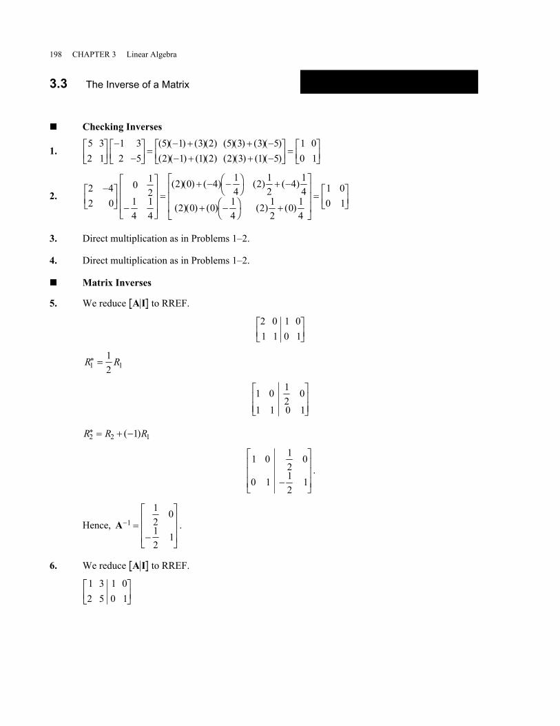
3.3 The Inverse of a Matrix
!!!! Checking Inverses
1.5 32 1
1 32 5
5 1 3 2 5 3 3 52 1 1 2 2 3 1 5
1 00 1
LNMOQP−
−LNMOQP =
( ) −( ) + ( )( ) ( )( ) + ( ) −( )( ) −( ) + ( )( ) ( )( ) + ( ) −( )LNM
OQP =LNMOQP
2.2 42 0
0 12
14
14
2 0 4 14
2 12
4 14
2 0 0 14
2 12
0 14
1 00 1
−LNMOQP −
L
NMMM
O
QPPP=( )( ) + −( ) −FH IK ( ) + −( )
( )( ) + ( ) −FHIK ( ) + ( )
L
N
MMM
O
Q
PPP= LNMOQP
3. Direct multiplication as in Problems 1–2.
4. Direct multiplication as in Problems 1–2.
!!!! Matrix Inverses
5. We reduce A I to RREF.
2 0 1 01 1 0 1LNM
OQP
R R1 112
∗ =
1 0 12
01 1 0 1
LNMM
OQPP
R R R2 2 11∗ = + −( )
1 0 12
0
0 1 12
1−
L
NMMM
O
QPPP
.
Hence, A− =−
L
NMMM
O
QPPP
1
12
0
12
1.
6. We reduce A I to RREF.
1 3 1 02 5 0 1LNM
OQP
SECTION 3.3 The Inverse of a Matrix 199
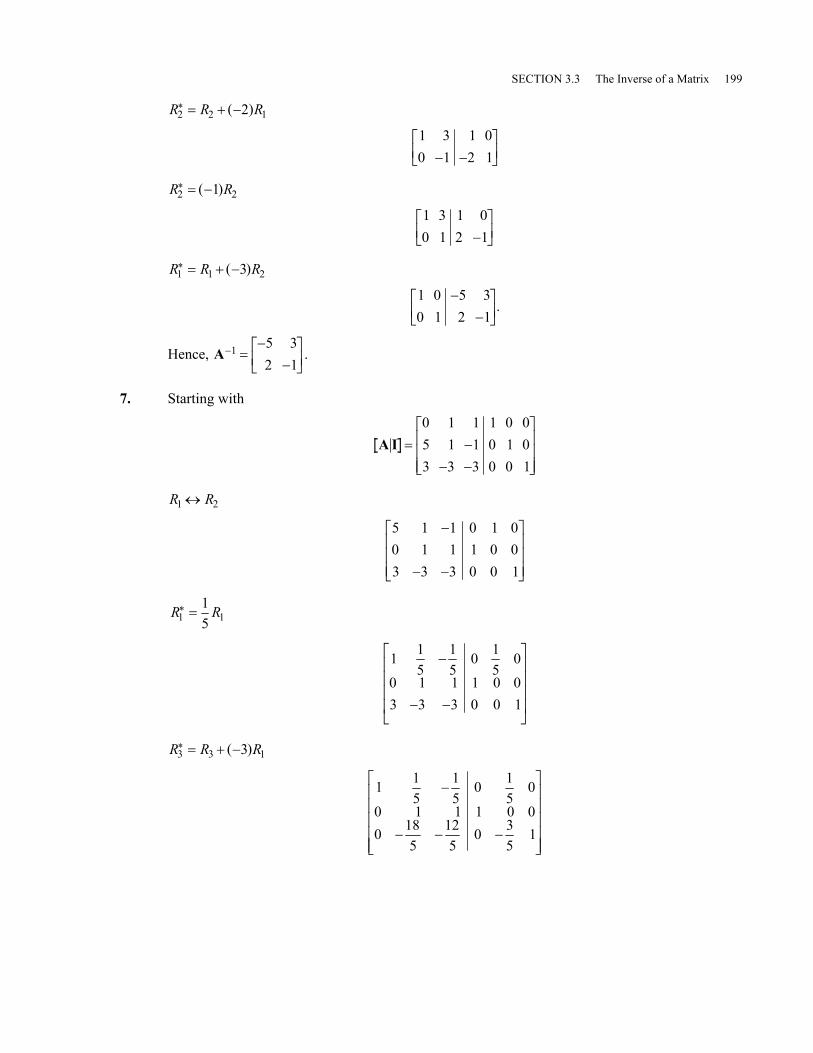
R R R2 2 12∗ = + −( )
1 3 1 00 1 2 1− −LNM
OQP
R R2 21∗ = −( )
1 3 1 00 1 2 1−LNM
OQP
R R R1 1 23∗ = + −( )
1 0 5 30 1 2 1
−−
LNM
OQP.
Hence, A− =−
−LNMOQP
1 5 32 1
.
7. Starting with
A I = −− −
L
NMMM
O
QPPP
0 1 1 1 0 05 1 1 0 1 03 3 3 0 0 1
R R1 2↔
5 1 1 0 1 00 1 1 1 0 03 3 3 0 0 1
−
− −
L
NMMM
O
QPPP
R R1 115
∗ =
1 15
15
0 15
00 1 1 1 0 03 3 3 0 0 1
−
− −
L
N
MMMM
O
Q
PPPP
R R R3 3 13∗ = + −( )
1 15
15
0 15
0
0 1 1 1 0 00 18
5125
0 35
1
−
− − −
L
N
MMMMM
O
Q
PPPPP
200 CHAPTER 3 Linear Algebra
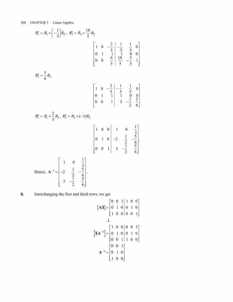
R R R1 1 215
∗ = + −FH IK , R R R3 3 2185
∗ = +
1 0 25
15
15
0
0 1 1 1 0 00 0 6
5185
35
1
− −
−
L
N
MMMMM
O
Q
PPPPP
R R3 356
∗ =
1 0 25
15
15
00 1 1 1 0 00 0 1 3 1
256
− −
−
L
N
MMMM
O
Q
PPPP
R R R1 1 325
∗ = + , R R R2 2 31∗ = + −( )
1 0 0 1 0 13
0 1 0 2 12
56
0 0 1 3 12
56
− −
−
L
N
MMMMMM
O
Q
PPPPPP
.
Hence, A− = − −
−
L
N
MMMMMM
O
Q
PPPPPP
1
1 0 13
2 12
56
3 12
56
.
8. Interchanging the first and third rows, we get
A I
I A
A
=L
NMMM
O
QPPP
B
=L
NMMM
O
QPPP
=L
NMMM
O
QPPP
−
−
0 0 1 1 0 00 1 0 0 1 01 0 0 0 0 1
1 0 0 0 0 10 1 0 0 1 00 0 1 1 0 00 0 10 1 01 0 0
1
1
SECTION 3.3 The Inverse of a Matrix 201
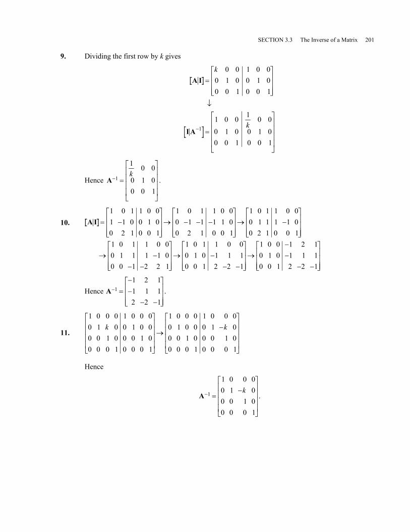
9. Dividing the first row by k gives
A I
I A
=L
NMMM
O
QPPP
B
=
L
N
MMMM
O
Q
PPPP−
k
k
0 0 1 0 00 1 0 0 1 00 0 1 0 0 1
1 0 0 1 0 00 1 0 0 1 00 0 1 0 0 1
1
Hence A− =
L
N
MMMM
O
Q
PPPP1
1 0 00 1 00 0 1
k.
10. A I = −L
NMMM
O
QPPP→ − − −L
NMMM
O
QPPP→ −L
NMMM
O
QPPP
→ −− −
L
NMMM
O
QPPP→ −
− −
L
NMMM
O
QPPP→
−−
− −
1 0 1 1 0 01 1 0 0 1 00 2 1 0 0 1
1 0 1 1 0 00 1 1 1 1 00 2 1 0 0 1
1 0 1 1 0 00 1 1 1 1 00 2 1 0 0 1
1 0 1 1 0 00 1 1 1 1 00 0 1 2 2 1
1 0 1 1 0 00 1 0 1 1 10 0 1 2 2 1
1 0 0 1 2 10 1 0 1 1 10 0 1 2 2 1
L
NMMM
O
QPPP
Hence A− =−−
− −
L
NMMM
O
QPPP
11 2 11 1 12 2 1
.
11.
1 0 0 0 1 0 0 00 1 0 0 1 0 00 0 1 0 0 0 1 00 0 0 1 0 0 0 1
1 0 0 0 1 0 0 00 1 0 0 0 1 00 0 1 0 0 0 1 00 0 0 1 0 0 0 1
k kL
N
MMMM
O
Q
PPPP→
−L
N
MMMM
O
Q
PPPP
Hence
A− =−
L
N
MMMM
O
Q
PPPP1
1 0 0 00 1 00 0 1 00 0 0 1
k.
202 CHAPTER 3 Linear Algebra
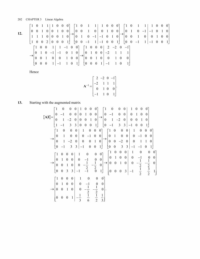
12.
1 0 1 1 1 0 0 00 0 1 0 0 1 0 01 1 1 0 0 0 1 01 0 0 2 0 0 0 1
1 0 1 1 1 0 0 00 0 1 0 0 1 0 00 1 0 1 1 0 1 00 0 1 1 1 0 0 1
1 0 1 1 1 0 0 00 1 0 1 1 0 1 00 0 1 0 0 1 0 00 0 1 1 1 0 0 1
1 0 0 1 1 1 0 00 1 0 1 1 0 1 00 0 1 0 0 1 0 00 0 0 1 1 1 0 1
L
N
MMMM
O
Q
PPPP→
− −− −
L
N
MMMM
O
Q
PPPP→
− −
− −
L
N
MMMM
O
Q
PPPP
→
−− −
−
L
N
MMMM
O
Q
PPPP→
− −−
−
L
N
MMMM
O
Q
PPPP
1 0 0 0 2 2 0 10 1 0 0 2 1 1 10 0 1 0 0 1 0 00 0 0 1 1 1 0 1
Hence
A− =
− −−
−
L
N
MMMM
O
Q
PPPP1
2 2 0 12 1 1 10 1 0 01 1 0 1
.
13. Starting with the augmented matrix
A I =−
−−
L
N
MMMM
O
Q
PPPP→
−−
− −
L
N
MMMM
O
Q
PPPP
→−
−− −
L
N
MMMM
O
Q
PPPP→
−−
−
1 0 0 0 1 0 0 00 1 0 0 0 1 0 00 1 2 0 0 0 1 01 1 3 3 0 0 0 1
1 0 0 0 1 0 0 00 1 0 0 0 1 0 00 1 2 0 0 0 1 00 1 3 3 1 0 0 1
1 0 0 0 1 0 0 00 1 0 0 0 1 0 00 1 2 0 0 0 1 00 1 3 3 1 0 0 1
1 0 0 0 1 0 0 00 1 0 0 0 1 0 00 0 2 0 0 1 1 00 0 3 3 1 −
L
N
MMMM
O
Q
PPPP
→−− −
− −
L
N
MMMM
O
Q
PPPP→
−− −
−
L
N
MMMMMM
O
Q
PPPPPP
→−− −
−
L
N
MMMMMM
O
Q
PPP
1 0 1
1 0 0 0 1 0 0 00 1 0 0 0 1 0 00 0 1 0 0 1
212
00 0 3 3 1 1 0 1
1 0 0 0 1 0 0 00 1 0 0 0 1 0 00 0 1 0 0 1
212
0
0 0 0 3 1 12
32
1
1 0 0 0 1 0 0 00 1 0 0 0 1 0 00 0 1 0 0 1
212
0
0 0 0 1 13
16
12
13
PPP
.

SECTION 3.3 The Inverse of a Matrix 203
Hence
A− =−− −
−
L
N
MMMMMM
O
Q
PPPPPP
1
1 0 0 00 1 0 00 1
212
013
16
12
13
.
!!!! Inverse of the 2 2× Matrix
14. Verify A A I AA− −= =1 1 . We have
A A I
AA I
−
−
=−
−−LNM
OQPLNMOQP = −
−−
LNM
OQP =
=LNMOQP −
−−LNM
OQP = −
−−
LNM
OQP =
1
1
1 1 00
1 1 00
ad bcd bc a
a bc d ad bc
ad bcad bc
a bc d ad bc
d bc a ad bc
ad bcad bc
Note that we must have A = − ≠ad bc 0.
!!!! Brute Force
15. To find the inverse of
1 31 2LNMOQP,
we seek the matrix
a bc dLNMOQP
that satisfies
a bc dLNMOQPLNMOQP =LNMOQP
1 31 2
1 00 1
.
Multiplying this out we get the equationsa b
a bc d
c d
+ =+ =+ =+ =
13 2 0
03 2 1.
The top two equations involve a and b, and the bottom two involve c and d, so we write the twosystems

204 CHAPTER 3 Linear Algebra
1 13 2
10
1 13 2
01
LNMOQPLNMOQP =LNMOQP
LNMOQPLNMOQP =LNMOQP
abcd
.
Solving each system, we get
ab
cd
LNMOQP =LNMOQPLNMOQP = −
−−LNMOQPLNMOQP =
−LNMOQP
LNMOQP =LNMOQPLNMOQP = −
−−LNMOQPLNMOQP = −LNMOQP
−
−
1 13 2
10
11
2 13 1
10
23
1 13 2
01
11
2 13 1
01
11
1
1
.
Because a and b are the elements in the first row of A−1, and c and d are the elements in thesecond row, we have
A−−
= LNMOQP =
−−
LNMOQP
111 3
1 22 31 1
.
!!!! Unique Inverse
16. We show that if B and C are both inverse of A, then B C= . Because B is an inverse of A, we canwrite BA I= . If we now multiply both sides on the right by C, we get
BA C IC C( ) = = .
But then we have
BA C B AC BI B( ) = ( ) = = , so B C= .
!!!! Invertible Matrix Method
17. Using the inverse found in Problem 6, yields
xx
1
2
1 5 32 1
410
5018
LNMOQP = =
−−
LNMOQP−LNMOQP = −LNMOQP
−A b .
!!!! Solution by Invertible Matrix
18. Using the inverse found in Problem 7, yields
xyz
L
NMMM
O
QPPP= = − −
−
L
N
MMMMMM
O
Q
PPPPPP
L
NMMM
O
QPPP= −L
NMMM
O
QPPP
−A b1
1 0 13
2 12
56
3 12
56
520
59
14.

SECTION 3.3 The Inverse of a Matrix 205
!!!! Noninvertible 2 2× Matrices
19. From Problem 14, the inverse of
A = LNMOQP
a bc d
can be written as
A− =−
−−LNMOQP
1 1ad bc
d bc a
,
which does not exist when ad bc− = 0 or ad bc= . Also, if we reduce A to RREF we get
1
0
ba
ad bca−
L
N
MMM
O
Q
PPP,
which says that the matrix is invertible when ad bca−
≠ 0 , or equivalently when ad bc≠ .
!!!! Cancellation Works
20. Given that AB AC= and A are invertible, we premultiply by A−1, getting
A AB A AC− −=1 1
or
IB IC= or B C= .
!!!! An Inverse
21. If A is an invertible matrix and AB I= , then we can premultiply each side of the equation byA−1 getting
A AB A I− −( ) =1 1
or
AA B A− −=1 1b g .
Hence, B A= −1.
!!!! Invertible Product
22. If AB is an invertible matrix, then there exists a matrix X that satisfies
AB X IA BX I( ) =( ) = .

206 CHAPTER 3 Linear Algebra
Hence, A has a right inverse BX. We also know
X AB IAB X
( ) =
= −1.
If we further assume that B is invertible then we can postmultiply this last equation by B−1,which yields
A X B BX= = ( )− − −1 1 1.
Now multiplying on the left by BX we have BX A I( ) = , which says that BX is also a left inverse
of A. Hence, the inverse of A exists and is BX.
!!!! Inconsistency
23. If Ax b= is inconsistent for some vector b, then A−1 does not exist because if A−1 did exist,then x A b= −1 exists for all b.
!!!! Elementary Matrices
24. (a) Eint =L
NMMM
O
QPPP
0 1 01 0 00 0 1
(b) Erepl =L
NMMM
O
QPPP
1 0 00 1 0
0 1k(c) Escale =
L
NMMM
O
QPPP
1 0 00 00 0 1
k
!!!! Invertibility of Elementary Matrices
25. Because the inverse of any elementary row operation is also an elementary row operation, andbecause elementary matrices are constructed from elementary row operations starting with theidentity matrix, we can convert any elementary row operation to the identity matrix byelementary row operations.
For example, the inverse of Eint can be found by performing the operation R R1 2↔ on
the augmented matrix
E Iint =L
NMMM
O
QPPP→L
NMMM
O
QPPP
0 1 0 1 0 01 0 0 0 1 00 0 1 0 0 1
1 0 0 0 1 00 1 0 1 0 00 0 1 0 0 1
.
Hence, Eint− =L
NMMM
O
QPPP
10 1 01 0 00 0 1
. In other words E Eint int= −1 . We leave finding Erepl−1 and Escale
−1 for the
reader.
SECTION 3.3 The Inverse of a Matrix 207
!!!! Leontief Model
26. T = LNMOQP
05 00 05.
., d = LNM
OQP
1010
The basic equation is
Total Output = External Demand + Internal Demand,
so we have
xx
xx
1
2
1
2
1010
05 00 05
LNMOQP =LNMOQP +LNMOQPLNMOQP
..
.
Solving these equations yields x x1 2 20= = . This should be obvious because for every 20 units of
product each industry produces, 10 goes back into the industry to produce the other 10.
27. T = LNMOQP
0 010 2 0
..
, d = LNMOQP
1010
The basic equation is
Total Output = External Demand + Internal Demand,
so we have
xx
xx
1
2
1
2
1010
0 0102 0
LNMOQP =LNMOQP +LNMOQPLNMOQP
..
.
Solving these equations yields x1 112= . , x2 12 2= . .
28. T = LNMOQP
02 0505 02. .. .
, d = LNMOQP
1010
The basic equation is
Total Output = External Demand + Internal Demand,
so we have
xx
xx
1
2
1
2
1010
02 0505 02
LNMOQP =LNMOQP +LNM
OQPLNMOQP
. .. .
.
Solving these equations yields x1 3313
= , x2 3313
= .
29. T = LNMOQP
05 0201 03. .. .
, d = LNMOQP
5050
The basic equation is
Total Output = External Demand + Internal Demand,

208 CHAPTER 3 Linear Algebra
so we have
xx
xx
1
2
1
2
5050
05 0201 03
LNMOQP =LNMOQP +LNM
OQPLNMOQP
. .
. ..
Solving these equations yields x1 1364= . , x2 909= . .
!!!! How Much Is Left Over?
30. The basic demand equation is
Total Output = External Demand + Internal Demand,
so we have
150250
03 0 405 03
150250
1
2
LNMOQP =LNMOQP +LNM
OQPLNMOQP
dd
. .
. ..
Solving for d1, d2 yields d1 5= , d2 100= .
!!!! Israeli Economy
31. (a) I T− = − −− −
L
NMMM
O
QPPP
0 70 000 0 00010 080 0 20005 001 0 98
. . .. . .. . .
(b) I T− =L
NMMM
O
QPPP
−b g 1143 0 00 0 000 20 125 0 260 07 0 01 102
. . .
. . .
. . .
(c) x I T d= −( ) =L
NMMM
O
QPPP
L
NMMM
O
QPPP=L
NMMM
O
QPPP
−1143 000 000020 125 026007 0 01 102
140 00020 0002,000
200520040
. . .
. . .
. . .
,,
$200,$53,$12,
!!!! Suggested Journal Entry
32. Student Project

SECTION 3.4 Determinants and Cramer’s Rule 209
3.4 Determinants and Cramer’s Rule
!!!! Calculating Determinants
1. Expanding by cofactors down the first column we get0 7 92 1 15 6 2
01 16 2
27 96 2
57 91 1
0− =−
− +−
= .
2. Expanding by cofactors across the middle row we get1 2 30 1 01 0 3
02 30 3
11 31 3
01 21 0
6−
=−
+−
− = − .
3. Expanding by cofactors down the third column we get
1 3 0 20 1 1 51 2 1 71 1 0 6
11 3 21 2 71 1 6
1 3 20 1 51 1 6
6 6 12
−−
− −−
=−
− −−
+−
−= + = .
4. Expanding by cofactors across the third row we get
1 4 2 24 7 3 53 0 8 05 1 6 9
34 2 27 3 51 6 9
81 4 24 7 55 1 9
3 14 8 250 2042
− −−
− −
=− −
−−
+− −
− −= ( ) + ( ) = .
!!!! Find the Properties
5. Subtract the first row from the second row in the matrix in the first determinant to get the matrixin the second determinant.
6. Factor out 3 from the second row of the matrix in the first determinant to get the matrix in thesecond determinant.
7. Interchange the two rows of the matrix.
!!!! Basketweave for 3 3×
8. Direct computation as in Problems 1–4.

210 CHAPTER 3 Linear Algebra
9.0 7 92 1 15 6 2
0 35 108 45 0 28 0− = − + − − − =
10.1 2 30 1 01 0 3
3 0 0 3 0 0 6−
= − + + − − − = −
11. By an extended basketweave hypothesis,
0 1 1 01 1 0 10 0 0 10 1 1 0
0 0 0 0 0 0 1 0 1= + + + − − − − = − .
However, the determinant is clearly 0 (because rows 1 equals row 4), so the basketweave methoddoes not generalize to dimensions higher than 3.
!!!! Triangular Determinants
12. We verify this for 4 4× matrices. Higher-order matrices follow along the same lines. Given theupper-triangular matrix
A =
a a a aa a a
a aa
11 12 13 14
22 23 24
33 34
44
00 00 0 0
,
we expand down the first column, getting
a a a aa a a
a aa
aa a a
a aa
a aa a
aa a a a
11 12 13 14
22 23 24
33 34
44
11
22 23 24
33 34
44
11 2233 34
4411 22 33 44
00 00 0 0
00 0
0= = = .
!!!! Think Diagonal
13. The matrix is upper triangular, hence the determinant is the product of the diagonal elements−
= −( )( )( ) = −3 4 00 7 60 0 5
3 7 5 105.

SECTION 3.4 Determinants and Cramer’s Rule 211
14. The matrix is a diagonal matrix, hence the determinant is the product of the diagonal elements.
4 0 00 3 00 0 1
2
4 3 12
6− = ( ) −( ) = − .
15. The matrix is lower triangular, hence the determinant is the product of the diagonal elements.
1 0 0 03 4 0 00 5 1 0
11 0 2 2
1 4 1 2 8−
−−
= ( )( ) −( )( ) = − .
16. The matrix is upper triangular, hence the determinant is the product of the diagonal elements.
6 22 0 30 1 0 40 0 13 00 0 0 4
6 1 13 4 312
−−
= ( ) −( )( )( ) = − .
!!!! Invertibility Test
17. The matrix does not have an inverse because its determinant is zero.
18. The matrix has an inverse because its determinant is nonzero.
19. The matrix has an inverse because its determinant is nonzero.
20. The matrix has an inverse because its determinant is nonzero.

212 CHAPTER 3 Linear Algebra
!!!! Product Verification
21. A
B
AB
A 2
B
AB
= LNMOQP
= LNMOQP
= LNMOQP
= LNMOQP = −
= LNMOQP =
= LNMOQP = −
1 23 41 01 13 27 41 23 41 01 1
1
3 27 4
2
Hence AB A B= .
22. A A
B B
AB AB
=L
NMMM
O
QPPP⇒ = −
= −−
L
NMMM
O
QPPP⇒ = −
=−
−
L
NMMM
O
QPPP⇒ =
0 1 01 0 01 2 2
2
1 2 31 2 00 1 1
7
1 2 01 2 31 8 1
14
Hence AB A B= .
!!!! Determinant of an Inverse
23. We have
1 1 1= = =− −I AA A A
and hence AA
− =1 1 .
!!!! Do Determinants Commute?
24. Because
AB A B B A BA= = = ,
then A B is a product of real or complex numbers.
!!!! Determinant of Similar Matrices
25. The key to the proof lies in the determinant of a product of matrices. If
A P BP= −1 ,
we use the general properties
AA
− =1 1 , AB A B=

SECTION 3.4 Determinants and Cramer’s Rule 213
shown in Problems 23 and 24, and write
A P BP P B PP
B P BP
P B= = = = =− −1 1 1 1 .
!!!! Determinant of An
26. (a) If An = 0 for some integer n, we have
A An n= = 0
or
A = 0.
Hence, A is noninvertible.
(b) If An ≠ 0 for some integer n, then
A An n= ≠ 0
for some integer n. This implies A ≠ 0 , so A is invertible. In other words, for everymatrix A either An = 0 for all positive integers n or it is never zero.
!!!! Determinants of Sums
27. An example is
A = LNMOQP
1 00 1
, B =−
−LNMOQP
1 00 1
,
so
A B+ = LNMOQP
0 00 0
,
which has the determinant
A B+ = 0,
whereas
A B= = 1,
so A B+ = 2 . Hence,
A B A B+ ≠ + .
214 CHAPTER 3 Linear Algebra
!!!! Determinants of Sums Again
28. Letting
A = LNMOQP
1 10 0
, B =− −LNMOQP
1 10 0
,
we get
A B+ = LNMOQP
0 00 0
.
Thus A B+ = 0. Also, we have A = 0, B = 0 , so
A B+ = 0.
Hence,
A B A B+ = + .
!!!! Scalar Multiplication
29. For a 2 2× matrix, we see
ka kaka ka
k a a k a a ka aa a
11 12
21 22
211 22
221 12
2 11 12
21 22= − = .
For an n n× matrix, A, we can factor a k out of each row getting k knA A= .
!!!! Inversion by Determinants
30. Given the matrix
A =L
NMMM
O
QPPP
1 0 22 2 31 1 1
the matrix of minors can easily be computed and is
M =− −− −− −
L
NMMM
O
QPPP
1 1 02 1 14 1 2
.
The matrix of cofactors ~A , which we get by multiplying the minors by −( ) +1 i j , is given by
~A M= −( ) =−
− −−
L
NMMM
O
QPPP
+11 1 02 1 14 1 2
i j .

SECTION 3.4 Determinants and Cramer’s Rule 215
Taking the transpose of this matrix gives
~AT =− −
−−
L
NMMM
O
QPPP
1 2 41 1 10 1 2
.
Computing the determinant of A, we get A = −1. Hence, we have the inverse
AA
A− = =−
− −−
L
NMMM
O
QPPP
1 11 2 41 1 10 1 2
~ T .
!!!! Determinants of Elementary Matrices
31. (a) If we interchange the rows of the 2 2× identity matrix, we change the sign of thedeterminant because
1 00 1
1= , 0 11 0
1= − .
For a 3 3× matrix if we interchange the first and second rows, we get0 1 01 0 00 0 1
1= − .
You can verify yourself that if any two rows of the 3 3× identity matrix areinterchanged, the determinant is –1.
For a 4 4× matrix suppose the ith and jth rows are interchanged and that wecompute the determinant by expanding by minors across one of the rows that was notinterchanged. (We can always do this.) The determinant is then
A M M M M= − + −a a a a11 11 12 12 13 13 14 14 .
But the minors M11, M12 , M13 , M14 are 3 3× matrices, and we know each of these
determinants is –1 because each of these matrices is a 3 3× elementary matrix with tworows changed from the identity matrix. Hence, we know 4 4× matrices with two rowsinterchanged from the identity matrix have determinant –1. The idea is to proceedinductively from 4 4× matrices to 5 5× matrices and so on.
(b) The matrix1 0 0
1 00 0 1kL
NMMM
O
QPPP
216 CHAPTER 3 Linear Algebra
shows what happens to the 3 3× identity matrix if we add k times the 1st row to the 2ndrow. If we expand this matrix by minors across any row we see that the determinant isthe product of the diagonal elements and hence 1. For the general n n× matrix adding ktimes the ith row to the jth row places a k in the jith position of the matrix with all otherentries looking like the identity matrix. This matrix is an upper-triangular matrix, and itsdeterminant is the product of elements on the diagonal or 1.
(c) Multiplying a row, say the first row, by k of a 3 3× matrixk 0 00 1 00 0 1
L
NMMM
O
QPPP
and expanding by minors across any row will give a determinant of k. Higher-ordermatrices give the same result.
!!!! Determinant of a Product
32. (a) If A is not invertible then A = 0. If A is not invertible then neither is AB, so AB = 0.Hence, it yields AB A B= because both sides of the equation are zero.
(b) We first show that EA E A= for elementary matrices E. An elementary matrix is one
that results in changing the identity matrix using one of the three elementary operations.There are three kinds of elementary matrices. In the case when E results in multiplying arow of the identity matrix I by a constant k, we have:
EA
A E A
=
L
N
MMMM
O
Q
PPPP⋅
L
N
MMMM
O
Q
PPPP=
L
N
MMMM
O
Q
PPPP= =
1 0 00 0
0 0 1
11 12 1
21 22 2
1 2
11 12 1
21 22 2
1 2
!!
! ! ! !!
!!
! ! ! !!
!!
! ! ! !!
ka a aa a a
a a a
a a aka ka ka
a a ak
n
n
n n nn
n
n
n n nn
In those cases when E is a result of interchanging two rows of the identity or by adding amultiple of one row to another row, the verification follows along the same lines.
Now if A is invertible it can be written as the product of elementary matrices
A E E E= −p p 1 1 … .
If we postmultiply this equation by B, we get
AB E E E B= −p p 1 1 … ,
so
AB E E E B E E E B A B= = =− −p p p p1 1 1 1 … … .

SECTION 3.4 Determinants and Cramer’s Rule 217
!!!! Cramer’s Rule
33. x yx y+ =+ =
2 22 5 0
To solve this system we write it in matrix form as
1 22 5
20
LNMOQPLNMOQP =LNMOQP
xy
.
Using Cramer’s rule, we compute the determinants
A
A
A
= =
= =
= = −
1 22 5
1
2 20 5
10
1 22 0
4
1
2 .
Hence, the solution is
x
y
= = =
= = − = −
AAAA
1
2
101
10
41
4.
34. x yx y+ =+ =
λ2 1
To solve this system we write it in matrix form as
1 11 2 1LNMOQPLNMOQP =LNMOQP
xy
λ.
Using Cramer’s rule, we compute the determinants
A
A
A
= =
= = −
= = −
1 11 2
1
11 2
2 1
11 1
1
1
2
λλ
λλ .
Hence, the solution is
x
y
= =−
= −
= =−
= −
AAAA
1
2
2 11
2 1
11
1
λ λ
λ λ .
218 CHAPTER 3 Linear Algebra
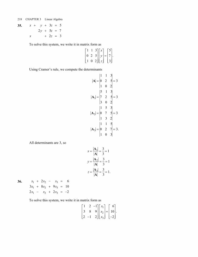
35. x y zy z
x z
+ + =+ =+ =
3 52 5 7
2 3
To solve this system, we write it in matrix form as1 1 30 2 51 0 2
573
L
NMMM
O
QPPP
L
NMMM
O
QPPP=L
NMMM
O
QPPP
xyz
.
Using Cramer’s rule, we compute the determinants
A
A
A
A
= =
= =
= =
= =
1 1 30 2 51 0 2
3
5 1 37 2 53 0 2
3
1 5 30 7 51 3 2
3
1 1 50 2 71 0 3
3
1
2
3 .
All determinants are 3, so
x
y
z
= = =
= = =
= = =
AAAAAA
1
2
3
33
1
33
1
33
1.
36. x x xx x xx x x
1 2 3
1 2 3
1 2 3
2 63 8 9 102 2 2
+ − =+ + =− + = −
To solve this system, we write it in matrix form as1 2 13 8 92 1 2
6102
1
2
3
−
−
L
NMMM
O
QPPP
L
NMMM
O
QPPP=−
L
NMMM
O
QPPP
xxx
.

SECTION 3.4 Determinants and Cramer’s Rule 219
Using Cramer’s rule, we compute the determinants
A
A
A
A
=−
−=
=−
− −=
=−
−=
=− −
= −
1 2 13 8 92 1 2
68
6 2 110 8 92 1 2
68
1 6 13 10 92 2 2
136
1 2 63 8 102 1 2
68
1
2
3 .
Hence, the solution is
x
x
x
11
22
33
6868
1
13668
2
6868
1
= = =
= = =
= = − = −
AAAAAA
.
!!!! The Wheatstone Bridge
37. (a) Each equation represents the fact that the sum of the currents into the respective nodes A,B, C, and D is zero. For example
node :node :node :node :
ABCD
I I I I I II I I I I II I I I I I
I I I I I I
g x g x
x x
g g
− − = ⇒ = +− − = ⇒ = +
− + + = ⇒ = ++ − = ⇒ = +
1 2 1 2
1 1
3 3
2 3 3 2
0000 .
(b) If a current I flows through a resistance R, then the voltage drop across the resistance isRI. Applying Kirchhoff’s voltage law, the sum of the voltage drops around each of thethree circuits is set to zero giving the desired three equations:
voltage drop around the large circuit E R I R Ix x0 1 1 0− − = ,
voltage drop around the upper-left circuit R I R I R Ig g1 1 2 2 0+ − = ,
voltage drop around the upper-right circuit R I R I R Ix x g g− − =3 3 0 .

220 CHAPTER 3 Linear Algebra
(c) Using the results from part (a) and writing the three currents I3, Ix , and I in terms of I1,I2 , Ig . gives
I I II I I
I I I
g
x g
3 2
1
1 2
= +
= −
= + .
We substitute these into the three given equations to obtain the 3 3× linear system forthe currents I1, I2 , Ig :
R R R R RR R R
R R R
III E
x x g
g
x x g
− − − −−
+ −
L
NMMM
O
QPPP
L
NMMM
O
QPPP=L
NMMM
O
QPPP
3 3
1 2
1
1
2
00
00 .
Solving for Ig (we only need to solve for one of the three unknowns) using Cramer’s
rule, we find
Ig =AA
1
where
A1
3
1 2
1 0
0 2 1 3
00
0=
−−
+
L
NMMM
O
QPPP= − +
R RR R
R R EE R R R R
x
x
xb g .
Hence, Ig = 0 if R R R Rx2 1 3= . Note: The proof of this result is much easier if we assumethe resistance Rg is negligible, and we take it as zero.
!!!! Least Squares Derivation
38. Starting with
F m k y k mxi ii
n, ( ) = − +
=∑ a f 2
1,
we compute the equations
∂∂
=Fk
0 , ∂∂
=Fm
0
yielding
∂∂
=∂∂
− + = − + −( ) =
∂∂
=∂∂
− + = − + − =
= =
= =
∑ ∑
∑ ∑
Fk k
y k mx y k mx
Fm m
y k mx y k mx x
i ii
n
i ii
n
i ii
n
i ii
n
i
a f a f
a f a f a f
2
1 1
2
1 1
2 1 0
2 0.

SECTION 3.4 Determinants and Cramer’s Rule 221
Carrying out a little algebra, we get
kn m x y
k x m x x y
ii
n
ii
n
ii
n
ii
n
i ii
n
+ =
+ =
= =
= = =
∑ ∑
∑ ∑ ∑
1 1
1
2
1 1
or in matrix form
n x
x x
km
y
x y
ii
n
ii
n
ii
n
ii
n
i ii
n=
= =
=
=
∑
∑ ∑
∑
∑
L
N
MMMM
O
Q
PPPPLNMOQP =L
N
MMMM
O
Q
PPPP1
1
2
1
1
1
.
!!!! Alternative Derivation of Least Squares Equations
39. (a) Equation (9) in the textk mk mk mk m
+ =+ =+ =+ =
17 112 3 3131 2 34 0 38
. .. .. .. .
can be written in matrix form
1 171 2 31 311 4 0
11312 338
....
.
...
L
N
MMMM
O
Q
PPPPLNMOQP =L
N
MMMM
O
Q
PPPPkm
which is the form of Ax b= .
(b) Given the matrix equation Ax b= , where
A =
L
N
MMMM
O
Q
PPPP
1111
1
2
3
4
xxxx
, x = LNMOQP
km
, b =
L
N
MMMM
O
Q
PPPP
yyyy
1
2
3
4
if we premultiply each side of the equation by AT, we get A Ax A bT T= , or
1 1 1 11111
1 1 1 1
1 2 3 4
1
2
3
4
1 2 3 4
1
2
3
4
x x x x
xxxx
km x x x x
yyyy
LNM
OQPL
N
MMMM
O
Q
PPPPLNMOQP =LNM
OQPL
N
MMMM
O
Q
PPPP
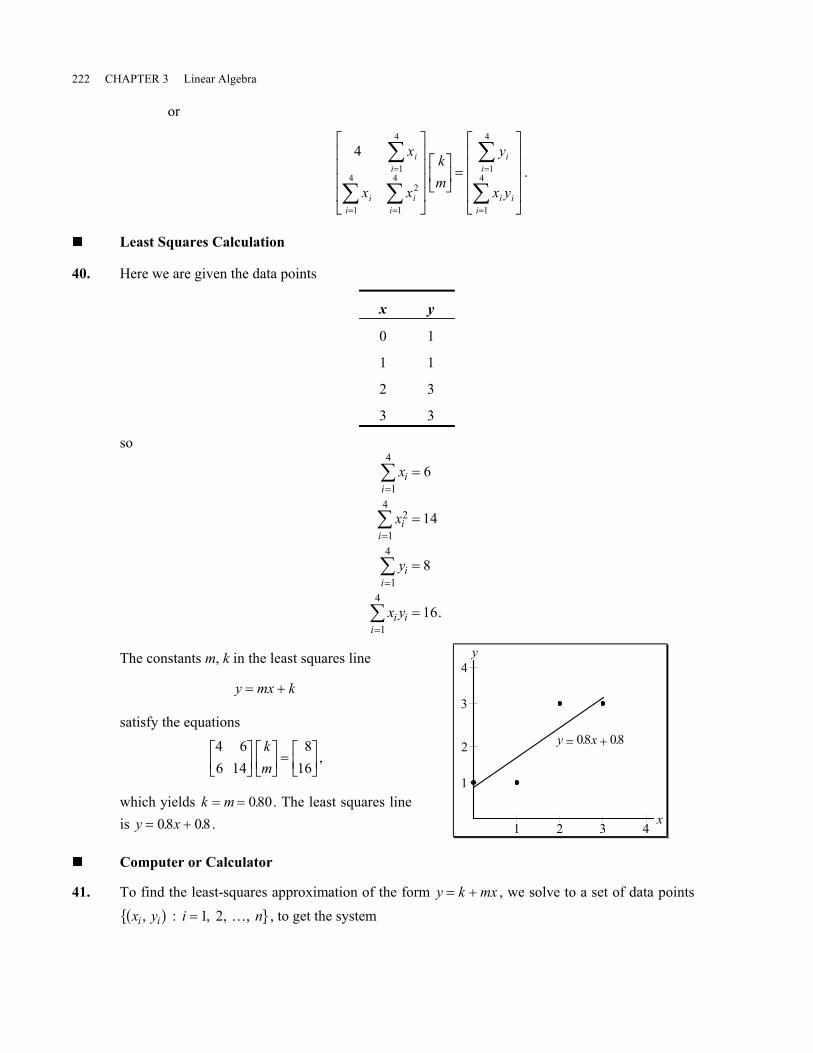
222 CHAPTER 3 Linear Algebra
or
41
4
1
42
1
41
4
1
4
x
x x
km
y
x y
ii
ii
ii
ii
i ii
=
= =
=
=
∑
∑ ∑
∑
∑
L
N
MMMM
O
Q
PPPPLNMOQP =L
N
MMMM
O
Q
PPPP.
!!!! Least Squares Calculation
40. Here we are given the data points
x y
0 1
1 1
2 3
3 3
so
x
x
y
x y
ii
ii
ii
i ii
=
=
=
=
∑
∑
∑
∑
=
=
=
=
1
4
2
1
4
1
4
1
4
6
14
8
16.
The constants m, k in the least squares line
y mx k= +
satisfy the equations
4 66 14
816
LNMOQPLNMOQP =LNMOQP
km
,
which yields k m= = 080. . The least squares lineis y x= +08 08. . . 42
2
1
3
4
1
3
y x= +08 08. .
x
y
!!!! Computer or Calculator
41. To find the least-squares approximation of the form y k mx= + , we solve to a set of data pointsx y i ni i, : , , a fk p= 1 2, … , to get the system
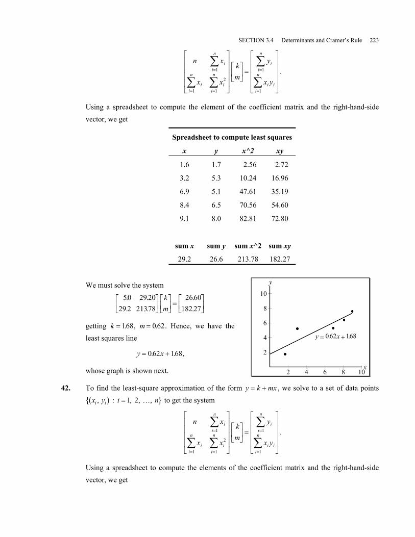
SECTION 3.4 Determinants and Cramer’s Rule 223
n x
x x
km
y
x y
ii
n
ii
n
ii
n
ii
n
i ii
n=
= =
=
=
∑
∑ ∑
∑
∑
L
N
MMMM
O
Q
PPPPLNMOQP =L
N
MMMM
O
Q
PPPP1
1
2
1
1
1
.
Using a spreadsheet to compute the element of the coefficient matrix and the right-hand-sidevector, we get
Spreadsheet to compute least squares
x y x^2 xy
1.6 1.7 2.56 2.72
3.2 5.3 10.24 16.96
6.9 5.1 47.61 35.19
8.4 6.5 70.56 54.60
9.1 8.0 82.81 72.80
sum x sum y sum x^2 sum xy
29.2 26.6 213.78 182.27
We must solve the system
50 29 2029 2 21378
26 60182 27
. .
. ...
LNM
OQPLNMOQP =LNMOQP
km
getting k = 168. , m = 0 62. . Hence, we have theleast squares line
y x= +0 62 168. . ,
whose graph is shown next. 84
4
2
6
8
2
6x
y
10
10
y x= +062 168. .
42. To find the least-square approximation of the form y k mx= + , we solve to a set of data pointsx y i ni i, : , , a fk p= 1 2, … to get the system
n x
x x
km
y
x y
ii
n
ii
n
ii
n
ii
n
i ii
n=
= =
=
=
∑
∑ ∑
∑
∑
L
N
MMMM
O
Q
PPPPLNMOQP =L
N
MMMM
O
Q
PPPP1
1
2
1
1
1
.
Using a spreadsheet to compute the elements of the coefficient matrix and the right-hand-sidevector, we get

224 CHAPTER 3 Linear Algebra
Spreadsheet to compute least squares
x y x^2 xy
0.91 1.35 0.8281 1.2285
1.07 1.96 1.1449 2.0972
2.56 3.13 6.5536 8.0128
4.11 5.72 16.8921 23.5092
5.34 7.08 28.5156 37.8072
6.25 8.14 39.0625 50.8750
sum x sum y sum x^2 sum xy
20.24 27.38 92.9968 123.5299
We must solve the system
600 20240020 24 92 9968
27 38001235299
. .
. ...
LNM
OQPLNMOQP =LNM
OQP
km
getting k = 0 309. , m = 126. . Hence, the least-squares line is y x= +0 309 126. . .
5
5
x
y
10
10
y x= +126 0309. .
!!!! Least Squares in Another Dimension
43. We seek the constants α, β1, and β2 that minimize
F y T Pi i ii
nα β β α β β, , 1 2 1 2
2
1a f a f= − + +
=∑ .
We write the equations
∂∂
= − + + −( ) =
∂∂
= − + + − =
∂∂
= − + + − =
=
=
=
∑
∑
∑
F y T P
F y T P T
F y T P P
i i ii
n
i i ii
n
i
i i ii
n
i
αα β β
βα β β
βα β β
2 1 0
2 0
2 0
1 21
11 2
1
21 2
1
a f
a f a f
a f a f .
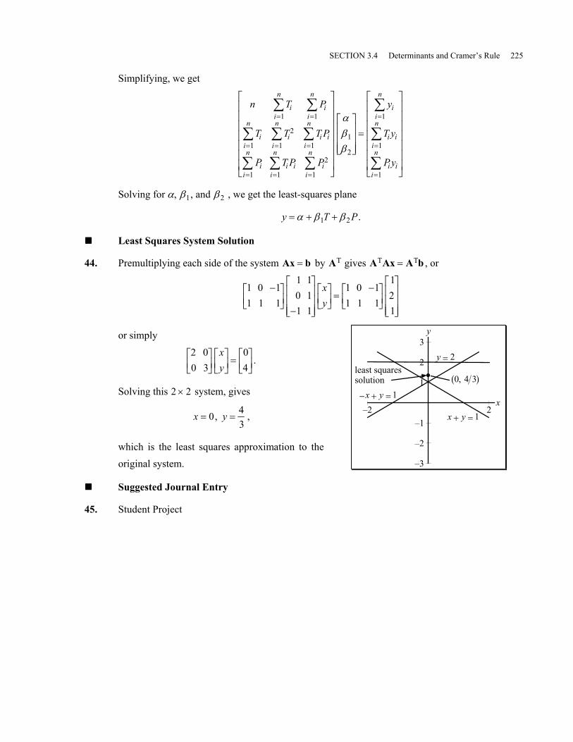
SECTION 3.4 Determinants and Cramer’s Rule 225
Simplifying, we get
n T P
T T T P
P T P P
y
T y
Py
ii
n
ii
n
ii
n
ii
n
i ii
n
ii
n
i ii
n
ii
n
ii
n
i ii
n
i ii
n
= =
= = =
= = =
=
=
=
∑ ∑
∑ ∑ ∑
∑ ∑ ∑
∑
∑
∑
L
N
MMMMMMM
O
Q
PPPPPPP
L
NMMM
O
QPPP=
L
N
MMMMMMM
O
Q
PPPPPPP
1 1
1
2
1 1
1 1
2
1
1
2
1
1
1
αββ
Solving for α, β1, and β2 , we get the least-squares plane
y T P= + +α β β1 2 .
!!!! Least Squares System Solution
44. Premultiplying each side of the system Ax b= by AT gives A Ax A bT T= , or
1 0 11 1 1
1 10 11 1
1 0 11 1 1
121
−LNM
OQP −
L
NMMM
O
QPPPLNMOQP =
−LNM
OQPL
NMMM
O
QPPP
xy
or simply
2 00 3
04
LNMOQPLNMOQP =LNMOQP
xy
.
Solving this 2 2× system, gives
x = 0, y = 43
,
which is the least squares approximation to theoriginal system.
2–1
–3
1
3
2
–2
–2
least squaressolution
y = 2
0 4 3,a f− + =x y 1
x y+ = 1
y
x
!!!! Suggested Journal Entry
45. Student Project

226 CHAPTER 3 Linear Algebra
3.5 Vector Spaces and Subspaces
!!!! They Don’t All Look Like Vectors
1. A typical vector is 1 2, ( ) , the zero vector is 0 0, ( ) and the negative of x y, ( ) is − −( )x y, .
2. A typical vector is 1 3 2, , ( ) , the zero vector is 0 0 0, , ( ) and the negative of x y z, , ( ) is− − −( )x y z, , .
3. A typical vector is 1 4, 3 0, , ( ) , the zero vector is 0 0 0 0, , , ( ) and the negative of a b c d, , , ( ) is− − − −( )a b c d, , , .
4. A typical vector is 1 3 9, , ( ) , the zero vector is 0 0 0, , ( ) and the negative of a b c, , ( ) is− − −( )a b c, , .
5. A typical vector is 1 9 02 3 0−LNM
OQP , the zero vector is
0 0 00 0 0LNMOQP and the negative of
a b cd e fLNM
OQP is
− − −− − −LNM
OQP
a b cd e f
.
6. A typical vector is 1 5 43 4 32 6 7
L
NMMM
O
QPPP, the zero vector is
0 0 00 0 00 0 0
L
NMMM
O
QPPP and the negative of
a b cd e fg h i
L
NMMM
O
QPPP
is
− − −− − −− − −
L
NMMM
O
QPPP
a b cd e fg h i
.
7. A typical vector is a linear function p t at b( ) = + , the zero vector is p ≡ 0 and the negative ofp t( ) is − ( )p t .
8. A typical vector is a linear function
p t at bt cb g = + +2 ,
the zero vector is p ≡ 0 and the negative of p t( )is − ( )p t .
4–4
–2
2
y
t
4
–4
–2 2
p t1( ) p t( )
p t3( )
p t2( )
Segments of typical vectors in P2

SECTION 3.5 Vector Spaces and Subspaces 227
9. A typical vector is a continuous and differenti-able function, such as f t t( ) = sin , the zero vectoris f t( ) ≡ 0 and the negative of f t( ) is − ( )f t .
4–4
–2
2
y
x
4
–4
–2 2
g t( )h t( )
f t( )
10. C 2 0 1, : Typical vectors are continuous and
twice differentiable functions such as
f t t( ) = sin , g t t t( ) = + −2 2 ,
and so on. The zero vector is the zero functionf t( ) ≡ 0, and the negative of a typical vector, sayf t e tt( ) = sin , is − ( ) = −f t e tt sin .
4
y
t
8
–4
–8
g t( )
f t( )
–4 4
f t( )
!!!! Are They Vector Spaces?
11. Not a vector space; there is no additive inverse.
12. First octant of space: No, the vectors have no negatives. For example, 1 3 3, , ( ) belongs to the setbut − − −( )1 3 3, , does not.
13. Not a vector space; e.g., the negative of (2, 1) does not lie in the set.
14. Not a vector space; e.g., x x2 + and −( )1 2x each belongs, but their sum x x x x2 21+ + −( ) = does
not.
15. Not a vector space, polynomial of degree 2.
16. Yes, a vector space, diagonal 2 × 2 matrices.
17. Not a vector space; the set is not closed under vector addition. 2 × 2 singular matrices: The set isnot closed under addition as indicated by
1 01 0
0 10 3
1 11 3
LNMOQP +LNMOQP =LNMOQP .
18. All invertible matrices: No, you can’t add matrices of different orders.
19. Yes, a vector space, 3 × 3 upper-triangular matrices.

228 CHAPTER 3 Linear Algebra
20. Not a vector space, does not contain the zero function. Continuous functions satisfying f 0 1( ) = .
21. Not a vector space; not closed under scalar multiplication; no additive inverse.
22. Yes, a vector space. All differentiable functions on −∞ ∞( ), .
23. Yes, a vector space. All integrable functions on 0 1, .
!!!! A Familiar Vector Space
24. Yes a vector space. Straightforward verification of the 10 commandments of a vector space; thatis, the sum of two vectors (real numbers in this case) is a vector (another real number), theproduct of a real number by a scalar (another real number) is a real number. The zero vector isthe number 0. Every number has a negative. The distributivity and associatively properties aresimply properties of the real numbers, and so on.
!!!! Not a Vector Space
25. Not a vector space; not closed under scalar multiplication.
!!!! DE Solution Space
26. Properties A3, A4, S1, S2, S3, and S4 are basic properties that hold for all functions; inparticular, solutions of a differential equation.
!!!! Another Solution Space
27. Yes, the solution space of the linear homogeneous DE
−( )′′ + ( ) − ′( ) + ( ) −( ) = − ′′ + ( ) ′ + ( ) =y p t y q t y y p t y q t y 0
is indeed a vector space; the linearity properties are sufficient to prove all the vector spaceproperties.
!!!! The Space C −∞ ∞( ),
28. This result follows from basic properties of continuous functions; the sum of continuous func-tions is continuous, scalar multiples of continuous functions are continuous, the zero function iscontinuous, the negative of a continuous function is continuous, the distributive properties holdfor all functions, and so on.
!!!! Vector Space Properties
29. Unique Zero: We prove that if a vector Z satisfies v Z v+ = for any vector v, then Z 0= . We canwrite
Z Z 0 Z v v Z v v v v 0= + = + + −( )( ) = +( ) + −( ) = + −( ) = .
SECTION 3.5 Vector Spaces and Subspaces 229
30. Unique Negative: We show that if v is an arbitrary vector in some vector space, then there is onlyone vector N (which we call –v) in that space that satisfies v N 0+ = . Suppose another vector ′Nalso satisfies v N 0+ ′ = . Then
N N 0 N v v N v v 0 v v N v v v N0 N N
= + = + + −( )( ) = +( ) + −( ) = + −( ) = + ′( ) + −( ) = + −( ) + ′= + ′ = ′ .
31. Zero as Multiplier: We can write
v v v v v v v+ = + = +( ) = =0 1 0 1 0 1 .
Hence, by the result of Problem 30, we can conclude that 0v 0= .
32. Negatives as Multiples: From Problem 30, we know that –v is the only vector that satisfiesv v 0+ −( ) = . Hence, if we write
v v v v v v 0+ −( ) = × + −( ) = + −( )( ) = × =1 1 1 1 1 0 .
Hence, we conclude that −( ) = −1 v v .
!!!! A Vector Space Equation
33. Let v be an arbitrary vector and c an arbitrary scalar. Set cv 0= . Then either c = 0 or v 0= . Forc ≠ 0,
v v v 0 0= = ( ) = ( ) =1 1 1c
cc
,
which proves the result.
!!!! Nonstandard Definitions
34. x y x y x x1 1 2 2 1 2 0, , , a f a f a f+ ≡ + , c x y cx y, , ( ) ≡ ( )
All vector space properties clearly hold for these operations. The set R2 with indicated vectoraddition and scalar multiplication is a vector space.
35. x y x y x1 1 2 2 20, , , a f a f a f+ ≡ , c x y cx cy, , ( ) ≡ ( )
Not a vector space because, for example, the new vector addition is not commutative:
2, 3 4, 0 4 5 ( ) + ( ) = ( ), , 4, 2, 3 0 2 5 ( ) + ( ) = ( ), .
36. x y x y x x y y1 1 2 2 1 2 1 2, , , a f a f a f+ ≡ + + , c x y cx cy, , ( ) ≡ d hNot a vector space, for example,
c d c d+( ) ≠ +x x x .
230 CHAPTER 3 Linear Algebra
For c = 4, d = 9 and vector x = x x1 2, a f, we have
c d x x x x
c d x x x x x x x x x x
+( ) = =
+ = + = + =
x
x x
13 13 13
4 9 2 2 3 3 5 51 2 1 2
1 2 1 2 1 2 1 2 1 2
, ,
, , , , , .
a f d ha f a f a f a f a f
!!!! Sifting Subsets for Subspaces
37. W = =x y y,a fk p0 is a subspace of R2.
38. W = + =x y x y,a fl q2 2 1 is not a subspace of R2 because it does not contain the zero vector
(0, 0). It is also not closed under vector addition and scalar multiplication.
39. W = =x x x x1 2 3 3 0, ,a fk p is a subspace of R3.
40. W = ( ) ( ) ={ }p t p tdegree 2 is not a subspace of P2 because it does not contain the zero vectorp t( ) ≡ 0 .
41. W = ( ) ( ) ={ }p t p 0 0 is a subspace of P3.
42. W = ( ) ( ) ={ }f t f 0 0 is a subspace of C 0 1, .
43. W = ( ) ( ) = ( ) ={ }f t f f0 1 0 is a subspace of C 0 1, .
44. W = ( ) ( ) =zf t f t dta
b0{ } is a subspace of C a b, .
45. W = ( ) ′′ + ={ }f t f f 0 is a subspace of C2 0 1, .
46. W = ′′ + =f t f f( ) 1m r is not a subspace of C2 0 1, . It does not contain the zero vector y t( ) ≡ 0 .
It is also not closed under vector addition and scalar multiplication because the sum of twosolutions is not necessarily a solution. For example, y t1 1= + sin and y t2 1= + cos are both
solutions, but the sum
y y t t1 2 2+ = + +sin cos
is not a solution. Likewise 2 2 21y t= + sin is not a solution.
!!!! Hyperplanes as Subspaces
47. We select two arbitrary vectors
u = x y z w1 1 1 1, , ,a f , v = x y z w2 2 2 2, , ,a ffrom the subset W. Hence, we have
ax by cz dwax by cz dw
1 1 1 1
2 2 2 2
00
+ + + =+ + + = .

SECTION 3.5 Vector Spaces and Subspaces 231
Adding, we get
a x x b y y c z z d w w ax by cz dw ax by cz dw1 2 1 2 1 2 1 2 1 1 1 1 2 2 2 2
0+ + + + + + + = + + + + + + +
=a f a f a f a f
which says that u v+ ∈W . To show ku ∈W , we must show that the scalar multiple
k kx ky kz kwu = 1 1 1 1, , ,a fsatisfies
akx bky ckz dkw1 1 1 1 0+ + + = .
But this follows from
akx bky ckz dkw k ax by cz dw1 1 1 1 1 1 1 1 0+ + + = + + + =a f .
!!!! Differentiable Subspaces
48. f t f( ) ′ ={ }0 . It is a subspace.
49. f t f( ) ′ ={ }1 . It is not a subspace, because it does not contain the zero vector and is not closedunder vector addition. Hence, f t t( ) = , g t t( ) = + 2 belongs to the subset but f g t+( )( ) does notbelong. It is also not closed under scalar multiplication. For example f t t( ) = belongs to thesubset, but 2 2f t t( ) = does not.
50. f t f f( ) ′ ={ } . It is a subspace.
51. f t f f( ) ′ = 2l q . It is not a subspace; e.g., not closed under scalar multiplication. ( f may satisfy
equation ′ =f f 2 , but 2f will not, since 2 4 2′ ≠f f .
!!!! Property Failures
52. The first quadrant (including the coordinate axes) is closed under vector addition, but not scalarmultiplications.
53. An example of a set in R2 that is closed under scalar multiplication but not under vector additionis that of two different lines passing through the origin.
54. The unit circle is not closed under either vector addition or scalar multiplication.
!!!! Nonlinear Differential Equations
55. ′ =y y2 . Writing the equation in differential form, we have y dy dt− =2 . We get the general
solution yc t
=−1 . Hence, from c = 0 and 1, we have two solutions
y tt11
( ) = − , y tt2
11
( ) =−
.

232 CHAPTER 3 Linear Algebra
But, if we compute
y t y tt t1 21 1
1( ) + ( ) = − +
−
it would not be a solution of the DE. So the solution set of this nonlinear DE is not a vectorspace.
56. ′′ + =y ysin 0 . Assume that y is a solution of the equation. Hence, we have the equation
′′ + =y ysin 0 .
But cy does not satisfy the equation because we have
cy cy c y y( )′′ + ( ) ≠ ′′ +( ) =sin sin 0 .
57. ′′ + =yy1 0 . From the DE we can see that the zero vector is not a solution, so the solution space
of this nonlinear DE is not a vector space.
!!!! Do They or Don’t They?
58. ′ + =y y et2 . Not a vector space, it doesn’t contain the zero vector.
59. ′ + =y y2 0 . The solutions are yt c
=−1 , and the sum of two solutions is not a solution, so the
general solution space of this nonlinear DE is not a vector space.
60. ′′ + =y ty 0 . If y1 , y2 satisfy the equation, then
′′+ =′′+ =
y tyy ty
1 1
2 2
00.
By adding, we obtain
′′+ + ′′ + =y ty y ty1 1 2 2 0a f a f ,
which from properties of the derivative is equivalent to
c y c y t c y c y1 1 2 2 1 1 2 2 0+ ′′ + + =a f a f .
This shows the set of solutions is a vector space.
61. ′′ + +( ) =y t y1 0sin . If y1 , y2 satisfy the equation then
′′+ +( ) =′′+ +( ) =
y t yy t y
1 1
2 2
1 01 0
sinsin .
By adding, we have
′′+ +( ) + ′′+ +( ) =y t y y t y1 1 1 11 1 0sin sin ,

SECTION 3.5 Vector Spaces and Subspaces 233
which from properties of the derivative is equivalent to
c y c y t c y c y1 1 2 2 1 1 2 21 0+ ′′ + +( ) + =a f a fsin ,
which shows the set of solutions is a vector space. This is true for the solution set of any linearhomogeneous DE.
!!!! Line of Solutions
62. (a) x p h= + = + = +t t t t0 1 2, 3 2 1 3, ,a f a f a fHence, calling x1 , x2 the coordinates of the vector x = x x1 2,a f , we have x t1 2= ,x t2 1 3= + .
(b) x = + −2, 1 3 2, 3 0, ,a f a ft
(c) Showing that solutions of ′ + =y y 0 are closed under vector addition is a result of the
fact that the sum of two solutions is a solution. The fact that solutions are closed underscalar multiplication is a result of the fact that scalar multiples of solutions are alsosolutions. The zero vector (zero function) is also a solution because the negative of asolution is a solution. Computing the solution of the equation gives y t ce t( ) = − , which is
scalar multiple of e t− . We will later discuss that this collection of solutions is a one-dimensional vector space.
(d) The solutions of ′ + =y y t are given by y t t ce t( ) = −( ) + −1 . The abstract point of view is
a line through the vector t −1 (remember functions are vectors here) in the direction ofthe vector e t− .
(e) The solution of any linear equation Ly f= can be interpreted as a line passing throughany particular solution yp in the direction of any homogeneous solution yh ; that is,y y cyp h= + .
!!!! Suggested Journal Entry
63. Student Project

234 CHAPTER 3 Linear Algebra
3.6 Bases and Dimension
!!!! The Spin on Spans
1. V R= 2 . Let
x y c cc c
c
, , ,,,
a f a f a fa fa f
= +==
1 2
2 2
2
0 0 1 1
1 1.
The given vectors do not span R2 , although they span the one-dimensional subspacek k1 1,a fk p ∈R .
2. V R= 3 . Letting
x y z c c c, , , , , , ,a f a f a f a f= + +1 2 31 0 0 0 1 0 2, 3 1
yields the system of equations
c c xc c y
c z
1 3
2 3
3
23
+ =+ =
=
or
c zc y c y zc x c x z
3
2 3
1 3
3 32 2
== − = −= − = − .
Hence, W spans R3.
3. V R= 3 . Letting
x y z c c c c, , , , , , , , ,a f a f a f a f a f= − + + − +1 2 3 41 0 1 2, 0 4 5 0 2 0 0 1
yieldsx c c cyz c c c c
= + −== − + + +
1 2 3
1 2 3 4
2 50
4 2 .
These vectors do not span R3 because they cannot give any vector with y ≠ 0 .
4. V P= 2 . Let
at bt c c c t c t t21 2 3
21 1 2 3+ + = ( ) + +( ) + − +b g .

SECTION 3.6 Bases and Dimension 235
Setting the coefficients of t2 , t, and 1 equal to each other gives
t c at c c b
c c c c
23
2 3
1 2 3
21 3
:::
=− =
+ + =
which has the solution c c b a1 5= − − , c b a2 2= + , c a3 = . Any vector in V can be written as a
linear combination of vectors in W. Hence, the vectors in W span V.
5. V P= 2 . Let
at bt c c t c t c t t21 2
23
21 1+ + = +( ) + + + −b g b g .Setting the coefficients of t2 , t, and 1 equal to each other gives
t c c at c c b
c c c
22 3
1 3
1 21
::: .
+ =− =
+ =
If we add the first and second equations, we get
c c a bc c c
1 2
1 2
+ = ++ =
This means we have a solution only if c a b= + . In other words, the given vectors do not spanP2 ; they only span a one-dimensional vector space of R3.
6. V M= 22 . Letting
a bc d
c c c cLNMOQP =LNMOQP +LNMOQP +LNMOQP +LNMOQP1 2 3 4
1 10 0
0 01 1
1 01 0
0 10 1
we have the equations
c c ac c bc c cc c d
1 3
1 4
2 3
2 4
+ =+ =+ =+ = .
If we add the first and last equation, and then the second and third equations, we obtain theequations
c c c c a dc c c c b c1 2 3 4
1 2 3 4
+ + + = ++ + + = + .
Hence, we have a solution if and only if a d b c+ = + . This means we can solve for c1 , c2 , c3 ,
c4 for only a subset of vectors in V. Hence, W does not span R4.

236 CHAPTER 3 Linear Algebra
!!!! Independence Day
7. V R= 2 . Setting
c c1 21 1 1 1 0 0, , ,− + − =a f a f a fwe get
c cc c1 2
1 2
00
− =− + =
which does not imply c c1 2 0= = . Hence, the vectors in W are linearly dependent.
8. V R= 2 . Setting
c c1 21 1 1 1 0 0, , ,a f a f a f+ − =
we get
c cc c1 2
1 2
00
+ =− =
which implies c c1 2 0= = . Hence, the vectors in W are linearly independent.
9. V R= 3 . Setting
c c c1 2 31 0 0 1 1 0 1 1 1 0 0 0, , , , , , , ,a f a f a f a f+ + =
we get
c c cc c
c
1 2 3
2 3
3
000
+ + =+ =
=
which implies c c c1 2 3 0= = = . Hence vectors in W are linearly independent.
10. V R= 3 . Setting
c c1 22, 1 4 4, 2, 8 0 0 0− + − =, , ,a f a f a fwe get
2 4 02 0
4 8 0
1 2
1 2
1 2
c cc cc c
+ =− − =
+ =
which (the equations are all the same) has a nonzero solution c1 2= − , c2 1= . Hence, the vectors
in W are linearly dependent.

SECTION 3.6 Bases and Dimension 237
11. V R= 3 . Setting
c c c1 2 31 1 8 3 4, 2 7, 1 3 0 0 0, , , , , ,a f a f a f a f+ − + − =
we get
c c cc c cc c c
1 2 3
1 2 3
1 2 3
3 7 04 0
8 2 3 0
− + =+ − =+ + =
which has only the solution c c c1 2 3 0= = = . Hence, the vectors in W are linearly independent.
12. V P= 1. Setting
c c t1 2 0+ = ,
we get c1 0= , c2 0= . Hence, the vectors in W are linearly independent.
13. V P= 1. Setting
c t c t1 21 1 0+( ) + −( ) =
we get
c cc c1 2
1 2
00
+ =− =
which has a unique solution c c1 2 0= = . Hence, the vectors in W are linearly independent.
14. V P= 2 . Setting
c t c t1 2 1 0+ −( ) = ,
we get
c cc
1 2
2
00
− ==
which implies c c1 2 0= = . Hence, the vectors in W are linearly independent.
15. V P= 2 . Setting
c t c t c t1 2 321 1 0+( ) + −( ) + =
we get
c cc c
c
1 2
1 2
3
000
+ =− =
=
which implies c c c1 2 3 0= = = . Hence, the vectors in W are linearly independent.
238 CHAPTER 3 Linear Algebra
16. V P= 2 . Setting
c t c t c t t1 22
323 1 2 5 0+( ) + − + − − =b g b g
we get
3 5 00
2 0
1 2 3
1 3
2 3
c c cc c
c c
− − =− =+ =
which has the nonzero solution c1 1= − , c2 2= , c3 1= − . Hence, the vectors in W are linearly
dependent.
17. V D= 22 . Setting
ab
c c0
01 00 0
0 00 11 2
LNMOQP =LNMOQP +LNMOQP
we get c a1 = , c b2 = . Hence, these vectors are linearly independent and span D22 .
18. V D= 22 . Setting
ab
c c0
01 00 1
1 00 11 2
LNMOQP =LNMOQP + −LNMOQP
we get c c a1 2+ = , c c b1 2− = . We can solve these equations for c1 , c2 , and hence these vectors
are linearly independent and span D22 .
!!!! Function Space Dependence
19. S = −e et t,l q . We set
c e c et t1 2 0+ =− .
Because we assume this holds for all t, it holds in particular for t = 0 , 1, so
c cec e c
1 2
11
2
00
+ =+ =−
which has only the zero solution c c1 2 0= = . Hence, the functions are linearly independent.
20. S = e te t et t t, , 2l q . We assume
c e c te c t et t t1 2 3
2 0+ + =
for all t. We let t = 0 , 1, 2, so
SECTION 3.6 Bases and Dimension 239
cec ec ec
e c e c e c
1
1 2 32
12
22
3
00
2 4 0
=+ + =+ + =
which has only the zero solution c c c1 2 3 0= = = . Hence, these vectors are linearly independent.
21. S = sin , sin , sint t t2 3k p . Letting
c t c t c t1 2 32 3 0sin sin sin+ + =
for all t. In particular if we choose three values of t, say π6
, π4
, π2
, we obtain three equations to
solve for c1 , c2 , c3 , namely,
c c c
c c c
c c
1 2 3
1 2 3
1 3
12
32
0
22
22
0
0
FHIK +FHGIKJ + =
FHGIKJ + +
FHGIKJ =
− = .
We used Maple to compute the determinant of this coefficient matrix and found it to be
− +32
12
6 . Hence, the system is nonsingular, and the only solution is c c c1 2 3 0= = = . Thus,
sin t , sin2t , and sin3t are linearly independent.
22. S = 1 2 2, sin , cost tl q . Because
1 02 2− − =sin cost t
the vectors are linearly dependent.
23. S = − −( )1 1 1 2, ,t tn s . Setting
c c t c t1 2 321 1 0+ −( ) + −( ) =
we get for the coefficients of 1, t, t2 the system of equations
c c cc c
c
1 2 3
2 3
3
02 0
0
− + =− =
=
which has the only zero solution c c c1 2 3 0= = = . Hence, these vectors are linearly independent.

240 CHAPTER 3 Linear Algebra
24. S = −e e tt t, , coshl q . Because
cosh t e et t= + −12b g
we have that 2 0cosh t e et t− − =− is a nontrivial linear combination that is identically zero forall t. Hence, the vectors are linearly dependent.
25. S = sin , cos2 4, 2t tl q . Recall the trigonometric identity
sin cos2 12
1 2t t= −( ) ,
which can be rewritten as
2 14
4 2 02sin cost t− ( ) + = .
Hence, we have found a nontrivial linear combination of the three vectors that is identically zero.Hence, the three vectors are linearly dependent.
!!!! Independence Testing
26. We will show the only values for which
cee
cee
t
t
t
t1 2
22 00
LNMOQP +LNMOQP =LNMOQP
for all t are c c1 2 0= = and, hence, conclude that the vectors are linearly independent. If it is true
for all t, then it must be true for t = 0 (which is the easiest place to test), which yields the twolinear equations
c cc c1 2
1 2
2 00
+ =+ =
whose only solution is c c1 2 0= = . Hence, the vectors are linearly independent.
Another approach is to say the vectors are linearly independent because clearly there isno constant k such that one vector is k times the other vector for all t.
27. We will show that
ctt
ctt1 2
00
sincos
cossin
LNMOQP + −LNMOQP =LNMOQP
for all t implies c c1 2 0= = , and hence, the vectors are linearly independent. If it is true for all t,then it must be true for t = 0 , which gives the two equations c2 0= , c1 0= . This proves the
vectors are linearly independent.

SECTION 3.6 Bases and Dimension 241
Another approach is to say that the vectors are linearly independent because clearly thereis no constant k such that one vector is k times the other vector for all t.
28. We write
ceee
ceee
ceee
t
t
t
t
t
t
t
t
t1 2 3
2
2
22 2 3
000
L
NMMM
O
QPPP+L
NMMM
O
QPPP+L
NMMM
O
QPPP=L
NMMM
O
QPPP
−
−
for all t and see if there are nonzero solutions for c1 , c2 , and c3 . Because the preceding equation
is assumed true for all t, it must be true for t = 1 (testing at t = 0 won’t work because there AREnonzero solutions there), or
c e c e c ec e c e c ec e c e c e
1 21
32
1 21
32
1 2 32
02 2 3 0
0
+ + =+ + =+ + =
−
−
.
Writing this in matrix form gives
e e ee e e
e e e
ccc
−
−
L
NMMM
O
QPPP
L
NMMM
O
QPPP=L
NMMM
O
QPPP
1 2
1 2
2
1
2
3
2 2 3000
.
Evaluating the determinant of this matrix with Maple (do it yourself if you like) we obtain anonzero value (the exact value is unimportant), so the vectors are linearly independent.
Another approach is to say that the vectors are linearly independent simply by looking atthem because clearly it is impossible to write any one vector as a linear combination of the othertwo due to the nature of the exponents.
29. We write
ceee
ce
ec
eee
t
t
t
t
t
t
t
t1 2 3
8
8
84 0
2
2
000
−
−
−
−
−
−L
NMMM
O
QPPP+
−
L
NMMM
O
QPPP+L
NMMM
O
QPPP=L
NMMM
O
QPPP
for all t and see if there are nonzero solutions for c1 , c2 , c3 . Because the above equation is
assumed true for all t, it must be true for t = 0 , or
c c cc cc c c
1 2 3
1 3
1 2 3
2 04 0
2 0
+ + =− + =
− + = .

242 CHAPTER 3 Linear Algebra
Writing this in matrix form gives
1 1 24 0 11 1 2
000
1
2
3
−−
L
NMMM
O
QPPP
L
NMMM
O
QPPP=L
NMMM
O
QPPP
ccc
.
The determinant of the coefficient matrix is 18, so the only solution of this linear system isc c c1 2 3 0= = = , and thus the vectors are linearly independent.
!!!! Twins?
30. We have
span
span
cos sin , cos sin cos sin cos sincos sin
cos sinsin , cos .
t t t t c t t c t tc c t c c t
C t C tt t
+ − = +( ) + −( )
= + + −= +=
k p k pa f a fk pk pk p
1 2
1 2 1 2
1 2
!!!! Wronskian
31. We assume that the Wronskian function
W f g t f t g t f t g t, ( ) = ( ) ′( ) − ′( ) ( ) ≠ 0
for every t ∈ 0 1, . To show f and g are linearly independent on [0, 1], we assume thatc f t c g t1 2 0( ) + ( ) = for all t in the interval [0, 1]. Differentiating, we have
c f t c g t1 2 0′( ) + ′( ) =
on [0, 1]. Hence, we have the two equations
f t g tf t g t
cc
( ) ( )
′( ) ′( )LNM
OQPLNMOQP =LNMOQP
1
2
00
.
The determinant of the coefficient matrix is the Wronskian of f and g, which is assumed to benonzero on [0, 1]. Since c c1 2 0= = , the vectors are linearly independent.
!!!! Linearly Independent Exponentials
32. We compute the Wronskian of f and g:
W f g tf t g tf t g t
e eae be
be ae e b aat bt
at bta b t a b t a b t, b g b g b gb g b g b gb g b g b g=
′ ′= = − = − ≠+ + + 0
for any t. Hence, f and g are linearly independent.

SECTION 3.6 Bases and Dimension 243
!!!! Looking Ahead
33. The Wronksian is
We tee e t
e t te et t
t tt t t=
+( )= +( ) − =
112 2 2 .
Hence, the vectors are linearly independent.
!!!! Revisiting Linear Independence
34. The Wronskian is
We e ee e ee e e
ee e
e ee
e ee e
ee ee e
e e
t t t
t t t
t t t
tt t
t tt
t t
t tt
t t
t t
t t
= − =−
− +−
= − − − − + + = −
−
−
−
−
−
−
−
−
−
55 3
5 9
5 35 9
55 9
55 3
45 15 45 5 15 5 80
3
3
3
3
3
3
3
3
3
3 3b g b g b gHence, the vectors are linearly independent.
!!!! Getting on Base in R2
35. Not a basis because 1 1,a fk p does not span R2.
36. Is a basis because 1 2 2, 1, ,a f a fk p are linearly independent and span R2.
37. − −1 1 1 1, , ,a f a fk p Not a basis because − −1 1 1 1, , ,a f a fk pand are linearly dependent.
38. 1 0 1 1, , ,a f a fk p Is a basis because the vectors are linearly independent and span R2.
39. 1 0 0 1 1 1, , , , ,a f a f a fk p Not a basis because the vectors are linearly dependent.
40. 0 0 1 1 2, 2, , , ,a f a f a fk p Not a basis because the vectors are linearly dependent.
!!!! The Base for the Space
41. V R= 3 : Not a basis because the two vectors are not enough to span R3.
42. V R= 3 : Yes, these vectors are linearly independent and span R3.
43. V R= 3 : Not a basis because four vectors must be linearly dependent in R3.
44. V P= 2 : Clearly the two vectors t t2 3 1+ + and t t2 2 4− + are linearly independent because theyare not constant multiples of one another. To verify they do not span P2 , however, we set
c t t c t t at bt c12
22 23 1 2 4+ + + − + = + +b g b g .
244 CHAPTER 3 Linear Algebra
Comparing coefficients we get
c c ac c bc c c
1 2
1 2
1 2
3 24
+ =− =+ =
which can easily be seen to have no solution for arbitrary a, b, c. The two vectors are not a basisfor P2 . (Two vectors can never form a basis for a three-dimensional space.)
45. V P= 3: We assume that
c t c t c t c t c t t12
2 33
4 523 4 1 5 1 0+ +( ) + + + −( ) + − + =b g b g
and compare coefficients of t3 , t2 , t, 1. Not a basis because the five vectors must be linearlydependent in t3 , t2 , t, 1.
46. V P= 4 : We assume that
c t c t c t c t c t t14
2 33
4 523 4 1 5 1 0+ +( ) + + + −( ) + − + =b g b g
and compare coefficients. We find a homogeneous system of equations which has only the zerosolution c c c c c1 2 3 4 5 0= = = = = . Hence, the vectors are linearly independent. To show the
vectors span P4 , we set the above linear combination equal to an arbitrary vector
at bt ct dt e4 3 2+ + + + , and comparing coefficients arrive at a system equations, which can besolved for c1 , c2 , c3 , c4 , and c5 in terms of a, b, c, d, e. Hence, the vectors span P4 and
combined with linear independence are a basis for P4 .
47. V M= 22 . We assume that
c c c c1 2 3 41 00 0
0 10 0
0 01 0
1 11 1
0 00 0
LNMOQP +LNMOQP +LNMOQP +LNMOQP =LNMOQP
yields the equations
c cc c
c cc
1 4
2 4
3 4
4
0000
+ =+ =+ =
=
which has the zero solution c c c c1 2 3 4 0= = = = . Hence, the vectors are linearly independent. If
we replace the zero vector on the right of the preceding equation by an arbitrary vector
a bc dLNMOQP ,

SECTION 3.6 Bases and Dimension 245
we get the four equations
c c ac c b
c c cc d
1 4
2 4
3 4
4
+ =+ =+ =
=
This yields the solutionc dc c dc b dc a d
4
3
2
1
== −= −= −
Hence, the four given vectors span M22 . Because they are linearly independent and span M22 ,
they are a basis.
48. V M= 23: If we set a linear combination of these vectors to an arbitrary vector, like
c c c c ca b cd e f1 2 3 4 5
1 0 10 0 0
1 1 00 0 0
0 0 01 0 1
0 0 01 1 0
0 0 01 1 1
LNMOQP +LNMOQP +LNMOQP +LNMOQP +LNMOQP =LNM
OQP
we arrive at the algebraic equations
c c ac b
c cc c c d
c c ec c f
1 2
2
1
3 4 5
4 5
3 5
+ ===
+ + =+ =+ = .
Looking at the first three equations gives c a b1 = − , c c1 = . If we pick an arbitrary matrix such
that a b c− ≠ , we have no solution. Hence, the vectors do not span M22 and do not form a basis.
(They are linearly independent however.)
!!!! Sizing Them Up
49. W = + + =x x x x x x1 2 3 1 2 3 0, ,b gl qLetting x2 = α , x3 = β , we can write x1 = − −α β . Any vector in W can be written as
xxx
1
2
3
110
101
L
NMMM
O
QPPP=
− −L
NMMM
O
QPPP=
−L
NMMM
O
QPPP+
−L
NMMM
O
QPPP
α βαβ
α β
where α and β are arbitrary real numbers. Hence, The dimension of W is 2; a basis is
{ −1 1 0, ,a f , −1 0 1, ,a f}.

246 CHAPTER 3 Linear Algebra
50. W = + = =x x x x x x x x1 2 3 4 1 3 2 40, , , ,b gl qLetting x3 = α , x4 = β , we have
xxxx
1
2
3
4
= −===
αβαβ .
Any vector in W can be written as
xxxx
1
2
3
4
1010
0101
L
N
MMMM
O
Q
PPPP=
−L
N
MMMM
O
Q
PPPP=
−L
N
MMMM
O
Q
PPPP+
L
N
MMMM
O
Q
PPPP
αβαβ
α β
where α and β are arbitrary real numbers. Hence, the two vectors −1 0 1 0, , , and 0 1 0 1, , ,
form a basis of W, which is only two-dimensional.
!!!! Polynomial Dimensions
51. t t, −1k p . We write
at b c t c t+ = + −( )1 2 1
yielding the equations
t c c ac b
:: .
1 2
21+ =− =
We can represent any vector at b+ as some linear combination of t and t −1 . Hence, we havethat t t, −1k p spans a two-dimensional vector space.
52. t t t, ,− +1 12l q . We write
at bt c c t c t c t21 2 3
21 1+ + = + −( ) + +b gyielding the equations
t c at c c b
c c c
23
1 2
2 31
::: .
=+ =− + =
Because we can solve this system for c1 , c2 , c3 in terms of a, b, c getting
c a c bc a cc a
1
2
3
= − + += −=
the subspace spans the entire three-dimensional vector space P2 .

SECTION 3.6 Bases and Dimension 247
53. t t t2 2 1 1, ,− +n s . We write
at bt c c t c t c t21
22
231 1+ + = + − + +( )b g
getting the equations
t c c at c b
c c c
21 2
3
2 31
::: .
+ ==
− + =
Because we can solve this system for c1 , c2 , c3 in terms of a, b, c getting
c a b c1 = − + , c b c2 = − , c b3 = ,
the subspace spans the entire three-dimensional vector space P2 .
!!!! Basis for P2
54. We first show the vectors span P2 by selecting an arbitrary vector from P2 and show it can be
written as a linear combination of the three given vectors. We set
at bt c c t t c t c21
22 31 1+ + = + + + +( ) +b g
and try to solve for c1 , c2 , c3 in terms of a, b, c. Setting the coefficients of t2 , t, and 1 equal to
each other yields
t c at c c b
c c c c
21
1 2
1 2 31
::: ,
=+ =+ + =
giving the solutionc ac a bc b c
1
2
3
== − += − + .
Hence, the set spans P2 . We also know that the vectors
t t t2 1 1 1+ + +, ,l qare independent because setting
c t t c t c12
2 31 1 0+ + + +( ) + =b gwe get
cc cc c c
1
1 2
1 2 3
000
=+ =+ + =
248 CHAPTER 3 Linear Algebra
which has only the solution c c c1 2 3 0= = = . Hence, the vectors are a basis for P2 , for example,
3 2 1 3 1 1 1 1 12 2t t t t t+ + = + + − +( ) − ( )b g .
!!!! Two-by-Two Basis
55. Setting
c c c1 2 31 00 0
0 11 0
0 01 1
0 00 0
LNMOQP +LNMOQP +LNMOQP =LNMOQP
gives c1 0= , c2 0= , and c3 0= . Hence, the given vectors are linearly independent. If we add the
vector
0 01 0LNMOQP ,
then the new vectors are still linearly independent (similar proof), and an arbitrary 2 2× matrixcan be written as
a bc d
c c c cLNMOQP =LNMOQP +LNMOQP +LNMOQP +LNMOQP1 2 3 4
1 00 1
0 11 0
0 01 1
0 01 0
because it reduces to
c ac b
c dc c c c
1
2
3
2 3 4
===
+ + = .
This yields
c ac b
c dc b d
1
2
3
4
==== − −
in terms of a, b, c, and d and form a basis for M22 , which is four-dimensional.
!!!! Basis for Trace Zero Matrices
56. Letting
c c ca bc d1 2 3
1 00 1
0 10 0
0 01 0−
LNMOQP +LNMOQP +LNMOQP =LNMOQP
we find a c= 1 , b c= 2 , c c= 3 , d c= − 1 . Given a b c d= = = = 0 implies c c c c1 2 3 4 0= = = = ,
which shows the vectors (matrices) are linearly independent. It also shows they span the set of
SECTION 3.6 Bases and Dimension 249
2 2× matrices with trace zero because if a d+ = 0 , we can solve for c a d1 = = − , c b2 = , c c3 = .
In other words we can write any zero trace 2 2× matrix as follows as a linear combination of thethree given vectors (matrices):
a bc a
a b c−
LNMOQP = −LNMOQP +LNMOQP +LNMOQP
1 00 1
0 10 0
0 01 0
.
Hence, the vectors (matrices) form a basis for the 2 2× zero trace matrices.
!!!! Hyperplane Basis
57. Solving the equation
x y z w+ − + =3 2 6 0
for x we get
x y z w= − + −3 2 6 .
Letting y = α , z = β and w = γ , we can write
x = − + −3 2 6α β γ .
Hence, an arbitrary vector x y z w, , ,a f in the hyperplane can be written
xyzw
L
N
MMMM
O
Q
PPPP=
− + −L
N
MMMM
O
Q
PPPP=
−L
N
MMMM
O
Q
PPPP+
L
N
MMMM
O
Q
PPPP+
−L
N
MMMM
O
Q
PPPP
3 2 6 3100
2010
6001
α β γαβγ
α β γ .
The set of four-dimensional vectors
−L
N
MMMM
O
Q
PPPP
L
N
MMMM
O
Q
PPPP
−L
N
MMMM
O
Q
PPPP
RS||
T||
UV||
W||
3100
2010
6001
, ,
is a basis for the hyperplane.
!!!! Solution Basis
58. Letting z = α we solve for x and y, obtaining x = −4α , y = 5α . An arbitrary solution of the
system can be expressed asxyz
L
NMMM
O
QPPP=
−L
NMMM
O
QPPP=
−L
NMMM
O
QPPP
45
451
ααα
α .
Hence, the vector [–4, 5, 1] is a basis for the solutions.

250 CHAPTER 3 Linear Algebra
!!!! Cosets in R3
59. W = + + =x x x x x x1 2 3 1 2 3 0, ,a fk p, v = 0 0 1, ,a fWe want to write W in parametric form, so we solve the equation
x x x1 2 3 0+ + =
by letting x2 = β , x3 = γ and solving for x1 = − −β γ . These solutions can be written as
β γ β γ− + − ∈1 1 0 1 0 1, , , , : ,b g b gm r R ,
so the coset of (0, 0, 1) in W is the collection of vectors
0 0 1 1 1 0 1 0 1, , , , , , ,a f a f a fk p+ − + − ∈β γ β γ R .
Geometrically, this describes a plane passing through (0, 0, 1) and parallel to x x x1 2 3 0+ + = .
60. W = =x x x x1 2 3 3 0, ,a fk p , v = 1 1 1, ,a fHere a coset through the point (1, 1, 1) is given by the points
1 1 1 1 0 0 0 1 0, , , , , ,a f a f a fk p+ +β γ
where β and γ are arbitrary real numbers. This describes the plane through (1, 1, 1) parallel to
the x1 – x2 plane (i.e., the subspace W).
!!!! More Cosets
61. The coset through the point (1, –2, 1) is given by the points
1 2, 1 1 3 2, , ,− +a f a fk pt ;
t is an arbitrary number. This describes a line through (1, –2, 1) parallel to the line t 1 3 2, ,a f .!!!! Antiderivative Space
62. Because the general solution of the nth order equation d ydt
n
n = 0 is
y t c t c t c t cnn
nn( ) = + + + +−
−−
−1
12
21 0…
where c0 , c1 , … cn−1 are arbitrary constants, we have that the basis for the vector space of
solutions is given by
1 2 1, , ,t t tn… −l q .

SECTION 3.6 Bases and Dimension 251
!!!! DE Solution Space
63. The solutions of
′ − =y y2 0
are
y t ce t( ) = 2 ;
that is, all solutions are multiples of the continuous and differentiably-continuous function e t2 .Hence, the function e t2k p forms a basis for the solution set, which is a vector subspace of
C CR R( ) ( ), 1 , and so on.
!!!! Another Solution Space
64. If we solve the separable equation
′ − =y yt2 0
by separating variables, we get
dyy
tdt= 2 .
Hence,
ln y t c
y e e
y t e e c e
c t
c t t
= +
=
( ) = ± =
2
1
2
2 2
where c1 is an arbitrary constant. Hence, a basis for the solution set is et2n s . This vector space is
a subspace of many larger vector spaces including C −∞ ∞,a f and C2 −∞ ∞,a f .!!!! Line in Function Space
65. The general solution of ′ + = −y y e t2 2 is
y t ce tet t( ) = +− −2 2 .
We could say the solution is a “line” in the vector space of solutions, passing through te t−2 in thedirection of e t−2 .
!!!! Suggested Journal Entry I
66. Student Project

252 CHAPTER 3 Linear Algebra
!!!! Suggested Journal Entry II
67. Student Project
!!!! Suggested Journal Entry III
68. Student Project