Chapter 4Class 4

How strong is the linear relationship between the variables?

Correlation does not necessarily imply causality! Coefficient of correlation, r, measures degree of

association Values range from -1 to +1

Correlation

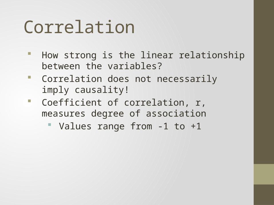
Correlation Coefficient

r = nSxy - SxSy

[nSx2 - (Sx)2][nSy2 - (Sy)2]

y

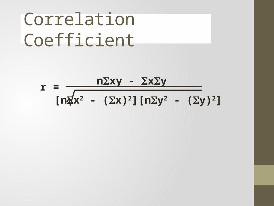
x(a) Perfect positive correlation: r = +1

y

x(b) Positive correlation: 0 < r < 1

y

x(c) No correlation: r = 0

y

x(d) Perfect negative correlation: r = -1

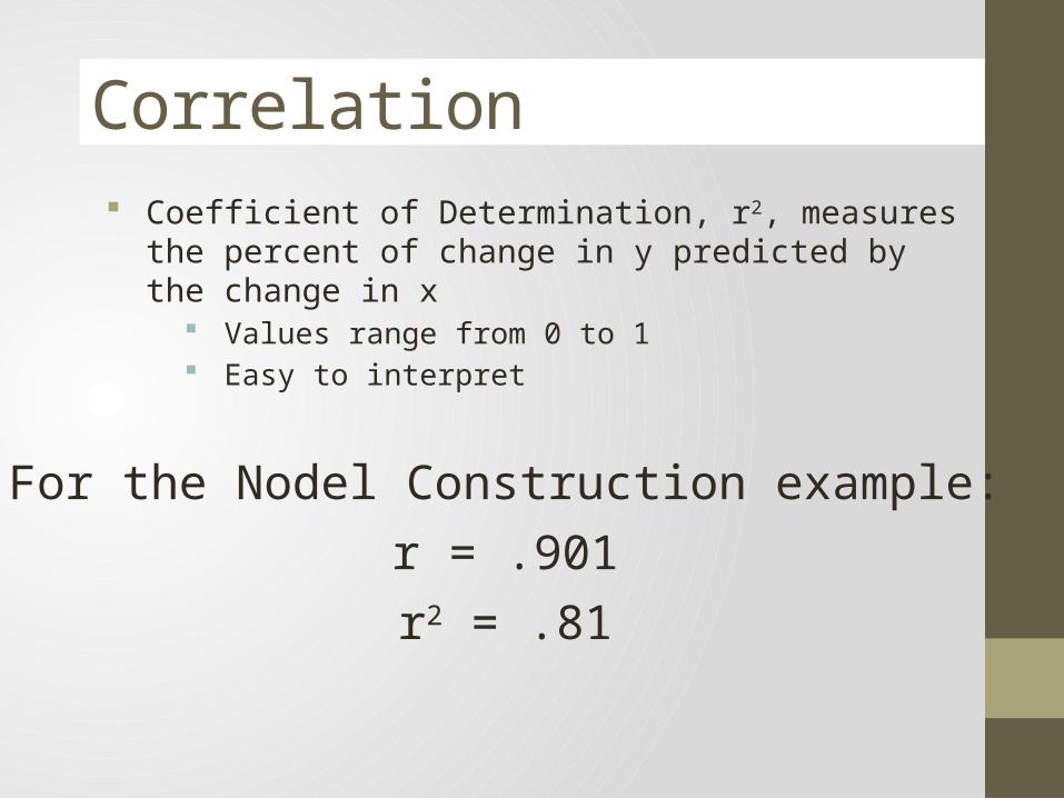
Coefficient of Determination, r2, measures the percent of change in y predicted by the change in x

Values range from 0 to 1 Easy to interpret

Correlation

For the Nodel Construction example:r = .901r2 = .81

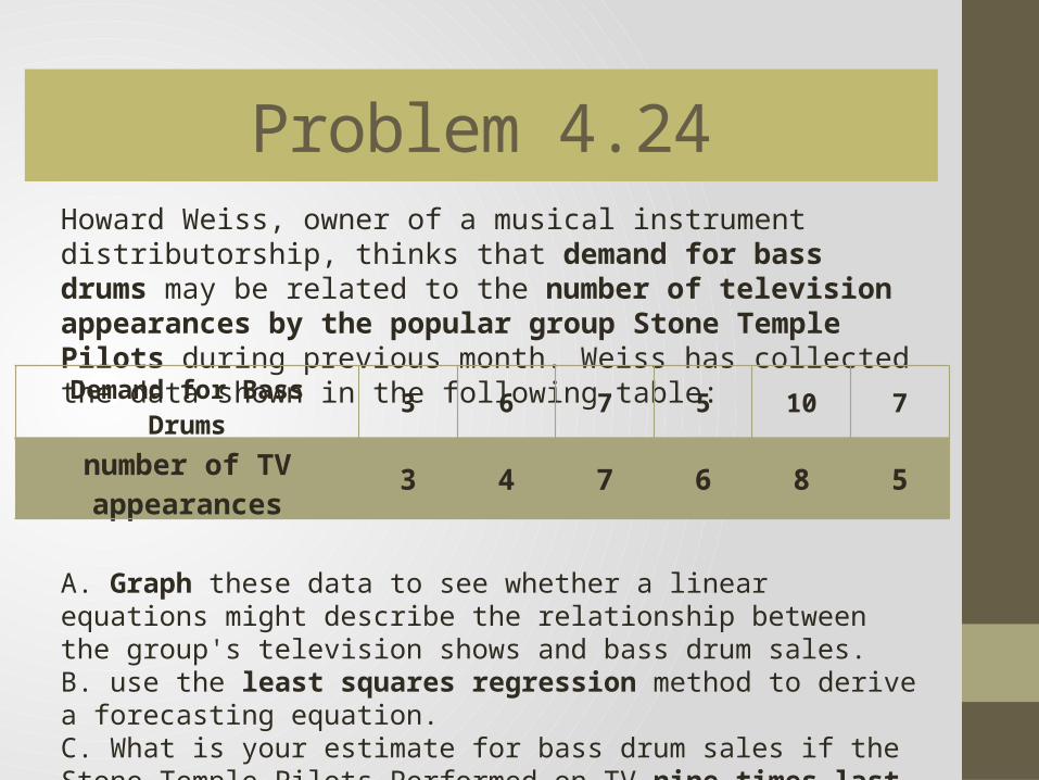
Problem 4.24Howard Weiss, owner of a musical instrument distributorship, thinks that demand for bass drums may be related to the number of television appearances by the popular group Stone Temple Pilots during previous month. Weiss has collected the data shown in the following table:

A. Graph these data to see whether a linear equations might describe the relationship between the group's television shows and bass drum sales.B. use the least squares regression method to derive a forecasting equation.C. What is your estimate for bass drum sales if the Stone Temple Pilots Performed on TV nine times last month?D. What are the correlation coefficient (r) and the coefficient of determination (r2) for this model, and what do they mean?

Demand for Bass Drums 3 6 7 5 10 7

number of TV appearances 3 4 7 6 8 5

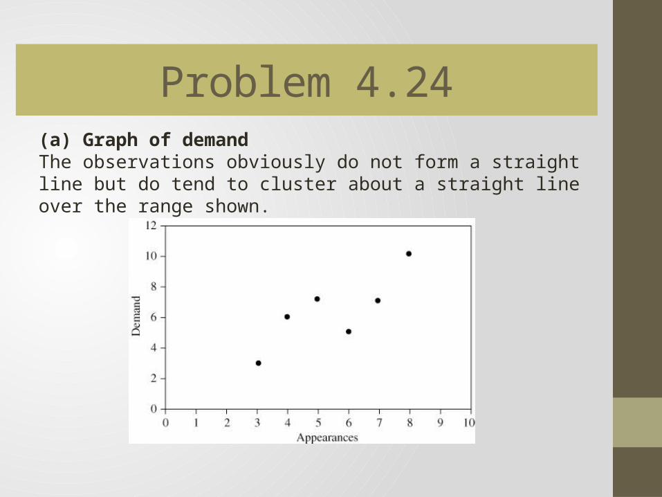
Problem 4.24(a) Graph of demandThe observations obviously do not form a straight line but do tend to cluster about a straight line over the range shown.

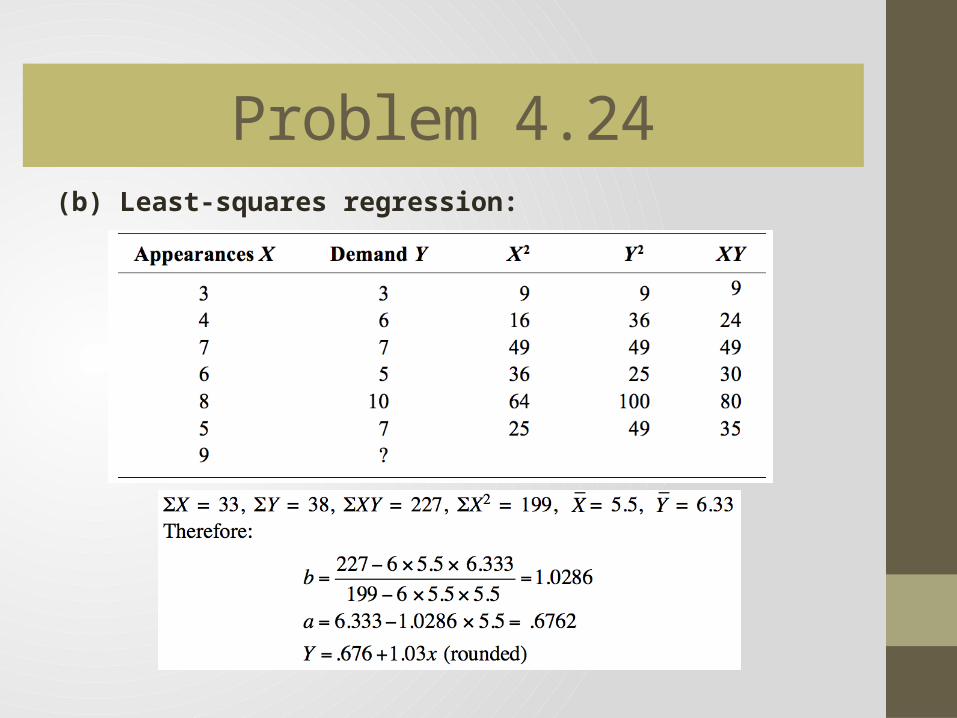
Problem 4.24(b) Least-squares regression:

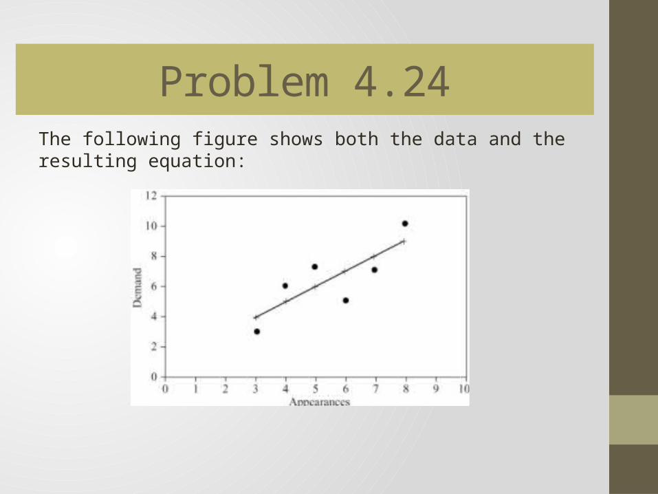
Problem 4.24The following figure shows both the data and the resulting equation:

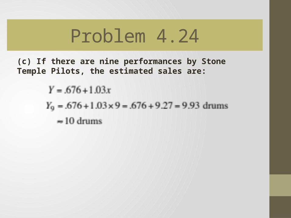
Problem 4.24(c) If there are nine performances by Stone Temple Pilots, the estimated sales are:

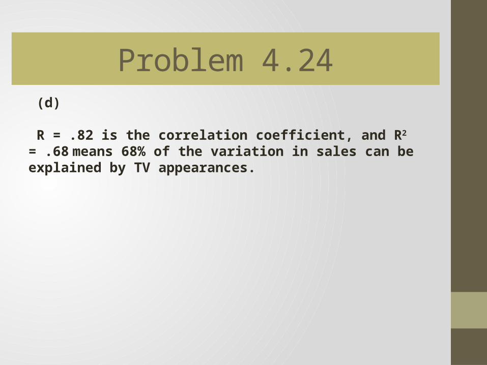
Problem 4.24 (d)

R = .82 is the correlation coefficient, and R2 = .68 means 68% of the variation in sales can be explained by TV appearances.

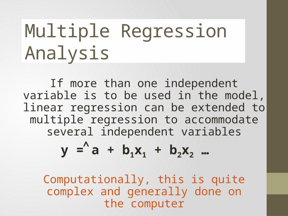
Multiple Regression Analysis

If more than one independent variable is to be used in the model, linear regression can be extended to

multiple regression to accommodate several independent variables

y = a + b1x1 + b2x2 …^

Computationally, this is quite complex and generally done on the computer

Multiple Regression Analysis

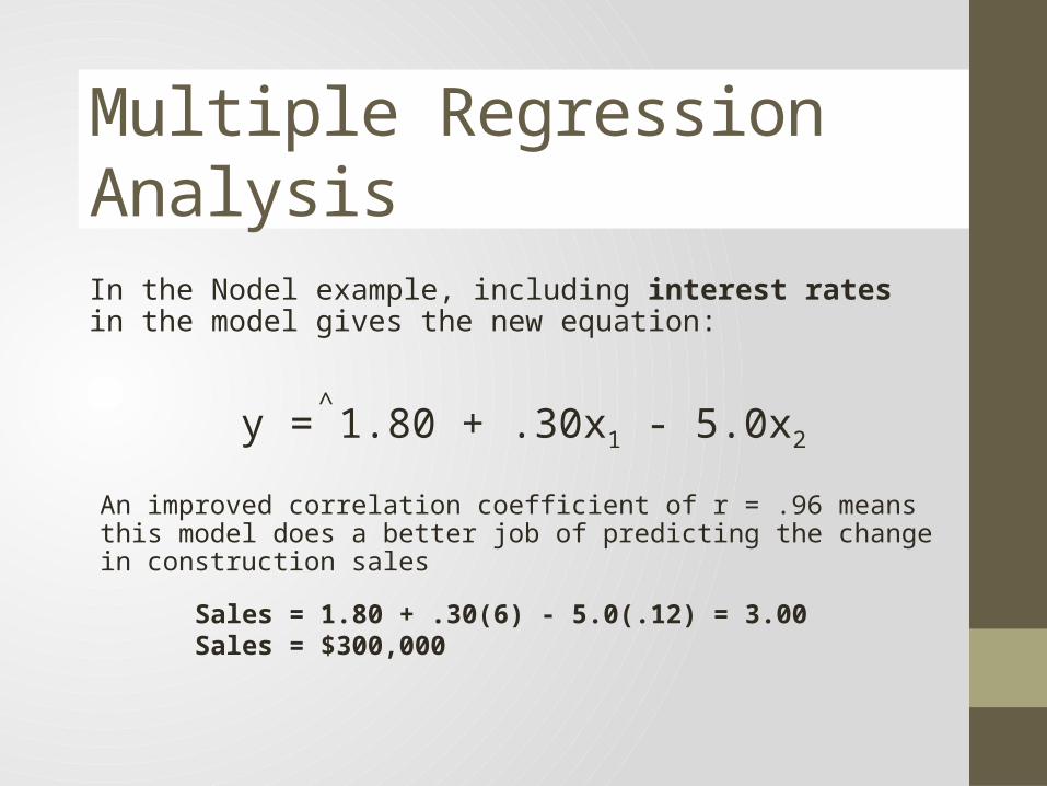
y = 1.80 + .30x1 - 5.0x2

^

In the Nodel example, including interest rates in the model gives the new equation:

An improved correlation coefficient of r = .96 means this model does a better job of predicting the change in construction sales

Sales = 1.80 + .30(6) - 5.0(.12) = 3.00Sales = $300,000

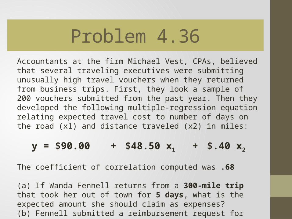
Problem 4.36Accountants at the firm Michael Vest, CPAs, believed that several traveling executives were submitting unusually high travel vouchers when they returned from business trips. First, they look a sample of 200 vouchers submitted from the past year. Then they developed the following multiple-regression equation relating expected travel cost to number of days on the road (x1) and distance traveled (x2) in miles:

y = $90.00 + $48.50 x1 + $.40 x2

The coefficient of correlation computed was .68

(a) If Wanda Fennell returns from a 300-mile trip that took her out of town for 5 days, what is the expected amount she should claim as expenses?(b) Fennell submitted a reimbursement request for $685. What should the accountant do?(c) Should any other variables be included? Which ones? Why?

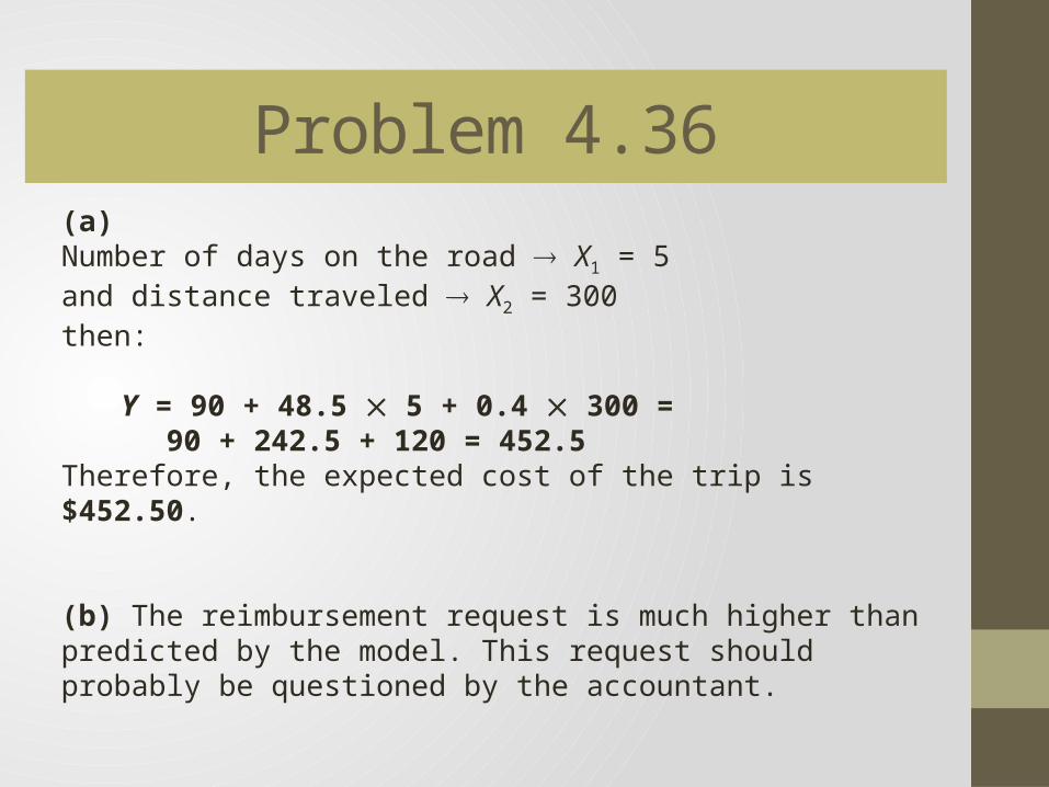
Problem 4.36(a)Number of days on the road X1 = 5 and distance traveled X2 = 300then:

Y = 90 + 48.5 5 + 0.4 300 = 90 + 242.5 + 120 = 452.5

Therefore, the expected cost of the trip is $452.50.

(b) The reimbursement request is much higher than predicted by the model. This request should probably be questioned by the accountant.

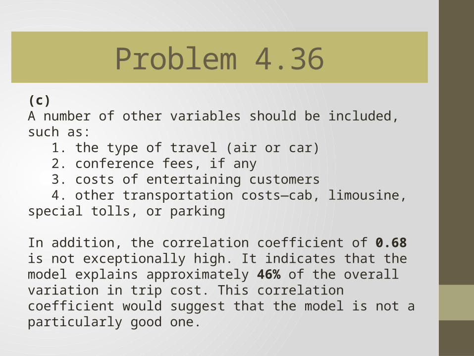
Problem 4.36(c) A number of other variables should be included, such as:

1. the type of travel (air or car)2. conference fees, if any3. costs of entertaining customers4. other transportation costs—cab, limousine, special tolls, or

parking

In addition, the correlation coefficient of 0.68 is not exceptionally high. It indicates that the model explains approximately 46% of the overall variation in trip cost. This correlation coefficient would suggest that the model is not a particularly good one.

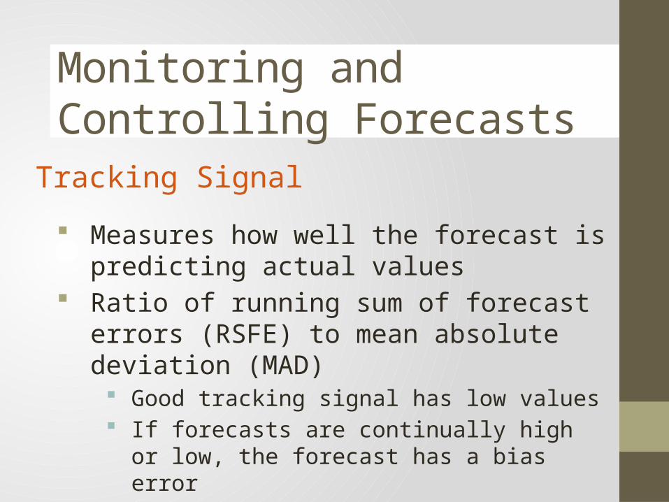
Measures how well the forecast is predicting actual values

Ratio of running sum of forecast errors (RSFE) to mean absolute deviation (MAD) Good tracking signal has low values If forecasts are continually high or low, the forecast

has a bias error

Monitoring and Controlling Forecasts

Tracking Signal

Monitoring and Controlling Forecasts

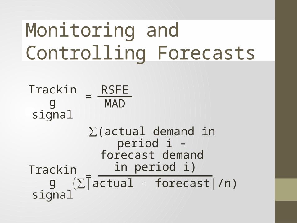
Tracking signal

RSFEMAD=

Tracking signal =

∑(actual demand in period i -

forecast demand in period i)

(∑|actual - forecast|/n)

Tracking Signal

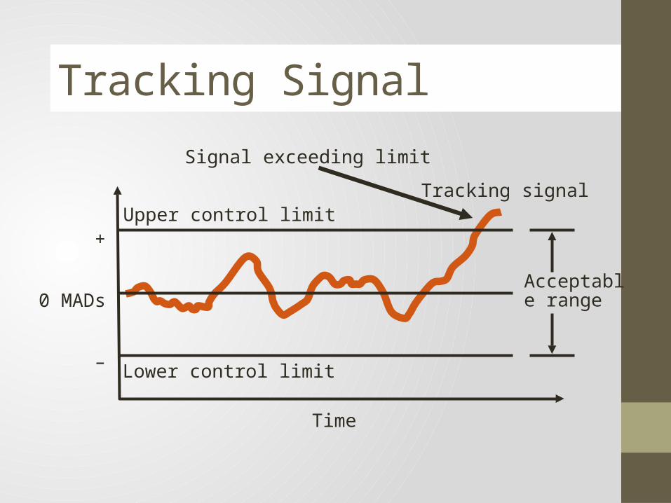
Tracking signal

+

0 MADs

–

Upper control limit

Lower control limit

Time

Signal exceeding limit

Acceptable range

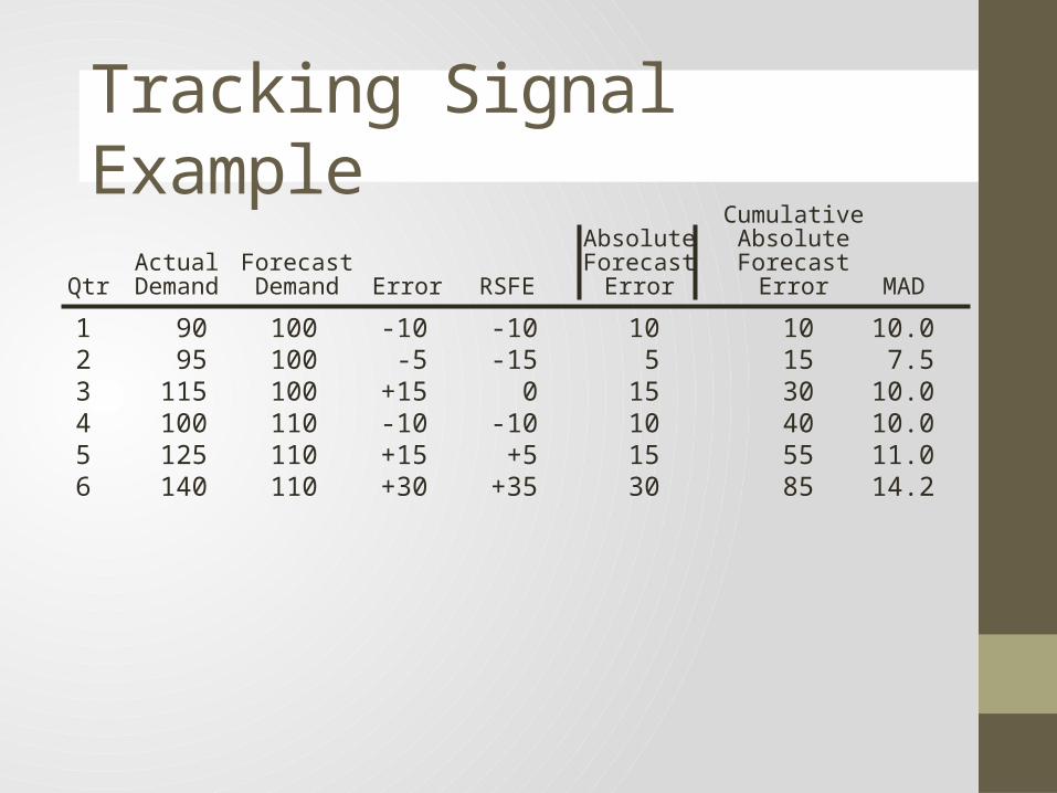
Tracking Signal ExampleCumulative

Absolute AbsoluteActual Forecast Forecast Forecast

Qtr Demand Demand Error RSFE Error Error MAD

1 90 100 -10 -10 10 10 10.02 95 100 -5 -15 5 15 7.53 115 100 +15 0 15 30 10.04 100 110 -10 -10 10 40 10.05 125 110 +15 +5 15 55 11.06 140 110 +30 +35 30 85 14.2

CumulativeAbsolute Absolute

Actual Forecast Forecast ForecastQtr Demand Demand Error RSFE Error Error MAD

1 90 100 -10 -10 10 10 10.02 95 100 -5 -15 5 15 7.53 115 100 +15 0 15 30 10.04 100 110 -10 -10 10 40 10.05 125 110 +15 +5 15 55 11.06 140 110 +30 +35 30 85 14.2

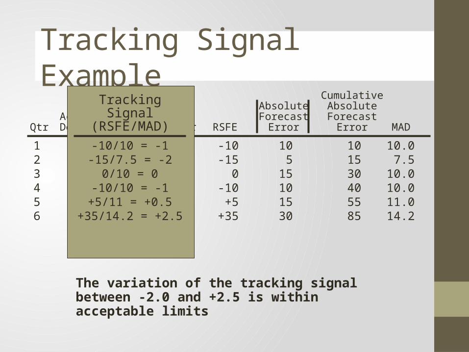
Tracking Signal ExampleTracking

Signal(RSFE/MAD)

-10/10 = -1-15/7.5 = -2

0/10 = 0-10/10 = -1

+5/11 = +0.5+35/14.2 = +2.5

The variation of the tracking signal between -2.0 and +2.5 is within acceptable limits

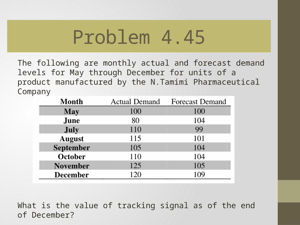
Problem 4.45The following are monthly actual and forecast demand levels for May through December for units of a product manufactured by the N.Tamimi Pharmaceutical Company

What is the value of tracking signal as of the end of December?

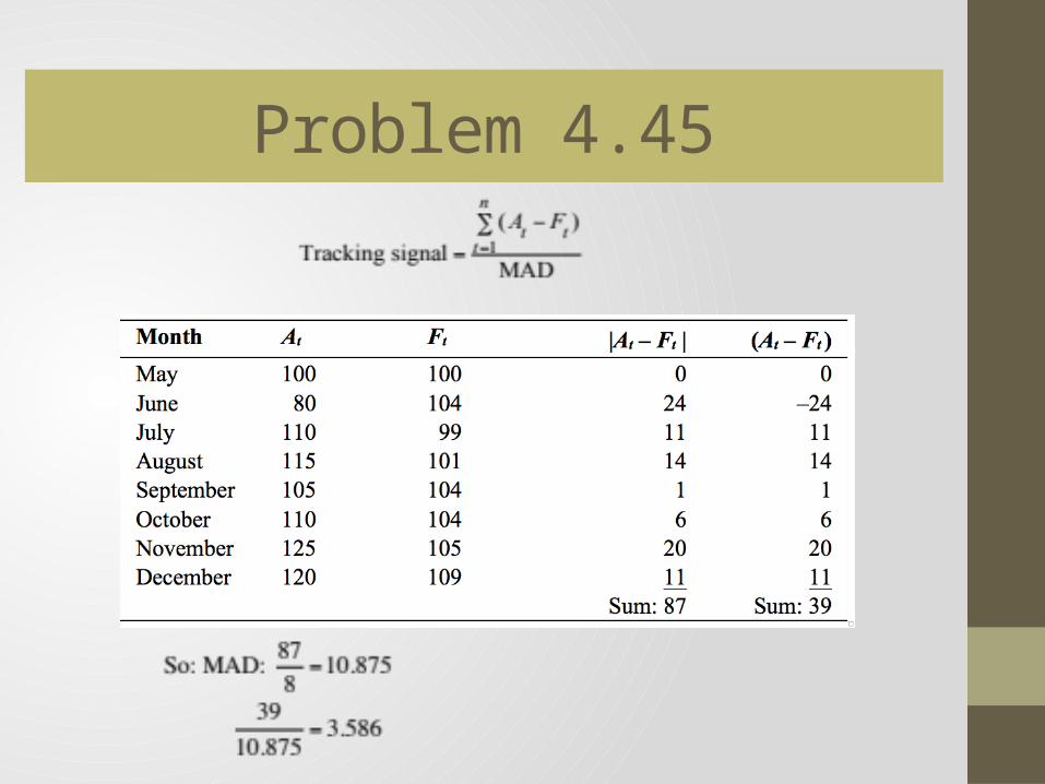
Problem 4.45