Embed Size (px)
Citation preview
113
CHAPTER 4
EXPERIMENTAL STUDIES
4.1 INTRODUCTION
Based on the results of the theoretical studies on the air-cooled GAX
based vapour absorption refrigeration system that were carried out, the design
and fabrication of the system have been done. The results of the pinch point
analysis helps to identify the streams responsible for heat recovery and
thereby heat load capacity for exchange between the streams. This helps to
design the internal heat recovery components such as high pressure GAX, low
pressure GAX, solution cooler, solution heat exchanger 2, condensate pre-
cooler. The heat load obtained for these components are used in the
experimental test-rig design. An experimental investigation of the
performance of the air-cooled GAX based vapour absorption refrigeration
system designed for 10.5 kW cooling capacity is presented. The experimental
plan and procedure, measurement of parameters and data reduction are
discussed in detail in this chapter.
4.2 COMPONENTS OF THE SYSTEM
The components of the air-cooled GAX based vapour absorption
refrigeration system, are the absorber, condenser, evaporator, generator, high
pressure GAX, low pressure GAX, solution heat exchanger 1, solution heat
exchanger 2, solution cooler and condensate pre-cooler. The components of
the air-cooled GAX based vapour absorption refrigeration system are
designed for the heat loads obtained from the thermodynamic analysis,

114
corresponding to a cooling capacity of 10.5 kW. At the designed conditions of
the generator, sink and evaporator temperatures of 150°C, 45°C and -10°C,
respectively and at a split factor of 0.8, based on the pinch point analysis, the
amount of heat recovered in the various internal heat exchanging components
are given in Table 4.1.
Table 4.1 Heat load of the internal heat exchanging components
ComponentHeat Load
(kW)
High Pressure GAX 3.6
Low Pressure GAX 4.6
Solution Heat Exchanger 1 12.2
Solution Heat Exchanger 2 3.6
Solution Cooler 5.3
Condensate Pre-Cooler 1.3
The components are designed using standard procedure with relevant heat and
mass transfer equations / coefficients. The specifications of the designed
components are given in Table 4.1. The component drawings are shown from
Figures 4.1 to 4.11.
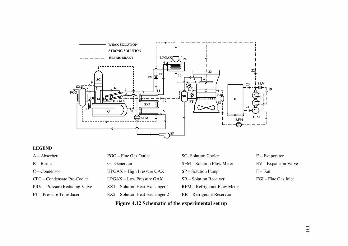
4.3 EXPERIMENTAL SET UP
All the components are fabricated as per design specifications, and
then assembled after testing for leaks. The schematic of the experimental
setup of the air-cooled GAX based vapour absorption refrigeration system is
shown in Figure 4.12.

115
Table 4.2 Specifications of the major components of the system
Component Design Conditions Specifications
Absorber
(Figure 4.1)
Weak solution temperature: 45°C
Strong solution temperature: 67 °C
Inlet air temperature: 28°C
Outlet air temperature: 38°C
Mass flow rate of weak solution: 0.058 kg/s
Mass flow rate of strong solution: 0.050 kg/s
Mass flow rate of refrigerant: 0.008 kg/s
Type: Finned
Material: Mild steel
Tube Diameter (ID): 15 mm
Thickness: 4 mm
Tube Length: 750 mm
Number of Tubes: 20
Heat Transfer Duty: 21.85
kW
Heat Transfer Area: 0.89 m2
Component Design Conditions Specifications
Condensor
(Figure 4.1)
Refrigerant vapour temperature: 48°C
Refrigerant liquid temperature: 46°C
Inlet air temperature: 28°C
Outlet air temperature: 38°C
Mass flow rate of refrigerant: 0.01 kg/s
Type: Finned
Material: Mild steel
Tube Diameter (ID): 15 mm
Thickness: 4 mm
Tube Length: 750mm
Number of Tubes: 16
Heat Transfer Duty: 11.96
kW
Heat Transfer Area: :0.72 m2

116
Table 4.2 (Contd….)
Component Design Conditions Specifications
Evaporator
(Figure 4.2)
Refrigerant liquid temperature: -12°C
Refrigerant vapour temperature: -10°C
Mass flow rate of refrigerant: 0.01 kg/s
Type: Shell and Coil
Material: Mild steel
Shell Diameter (OD): 600 mm
Shell Length: 1150 mm
Coil Diameter (OD): 25.4 mm
Thickness: 7.4 mm
Length: 1360 mm
Number of Coils: 28
Heat Transfer Duty: 10.5 kW
Heat Transfer Area: 5.77 m2
Component Design Conditions Specifications
Generator
(Figure 4.3)
Weak solution temperature: 119°C
Strong solution temperature: 150°C
Mass flow rate of weak solution: 0.058 kg/s
Mass flow rate of strong solution: 0.048 kg/s
Type: Direct Fired
Material: Mild steel
Diameter (ID): 488.6 mm
Diameter (OD): 514 mm
Length: 1552 mm
Heat Transfer Duty: 23.27 kW
Heat Transfer Area: 1 m2

117
Table 4.2 (Contd….)
Component Design Conditions Specifications
High Pressure
GAX
(Figure 4.4)
Weak solution inlet temperature: 45°C
Weak solution outlet temperature: 59°C
Refrigerant inlet temperature: 112°C
Refrigerant outlet temperature: 48°C
Mass flow rate of weak solution: 0.058 kg/s
Mass flow rate of refrigerant: 0.01 kg/s
Type: Shell and Tube
Material: Mild steel
Shell Diameter (ID): 103.5 mm
Thickness: 10.8 mm
Shell Length: 1194 mm
Tube Diameter (ID): 3.6 mm
Thickness: 2.4 mm
Tube Length: 1200 mm
Number of Tubes: 132
Heat Transfer Duty: 3.65 kW
Heat Transfer Area: 2.98 m2
Component Design Conditions Specifications
Low Pressure
GAX
(Figure 4.5)
Weak solution inlet temperature: 59°C
Weak solution outlet temperature: 68°C
Strong solution inlet temperature: 76°C
Strong solution outlet temperature: 67 °C
Refrigerant temperature: 38°C
Mass flow rate of weak solution: 0.058 kg/s
Mass flow rate of strong solution: 0.048 kg/s
Mass flow rate of refrigerant: 0.002 kg/s
Type: Shell and Tube
Material: Mild steel
Shell Diameter (ID): 303.2 mm
Thickness: 20.6 mm
Shell Length: 331 mm
Tube Diameter (ID): 3.6 mm
Thickness: 2.4 mm
Tube Length: 375 mm
Number of Tubes: 76
Heat Transfer Duty: 4.57 kW
Heat Transfer Area: 0.54 m2

118
Table 4.2 (Contd….)
Component Design Conditions Specifications
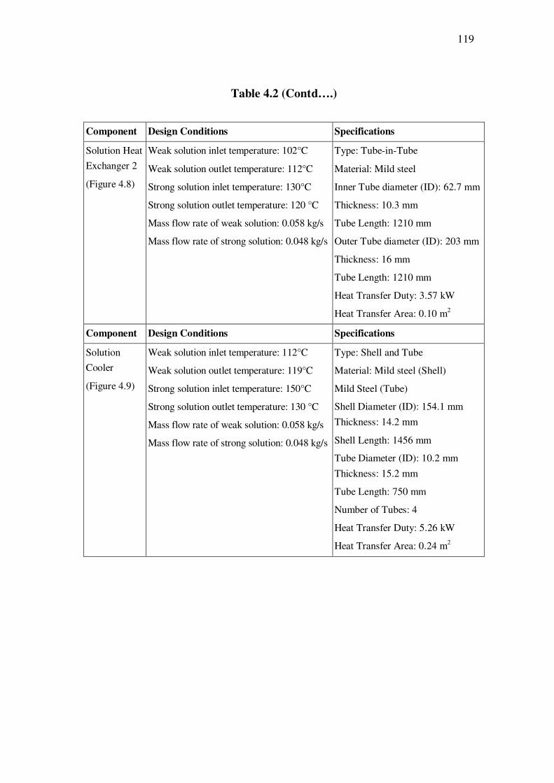
Condensate
Pre-Cooler
(Figure 4.6)
Refrigerant liquid inlet temperature: 46°C
Refrigerant liquid outlet temperature: 20°C
Refrigerant vapour inlet temperature: -10°C
Refrigerant vapour outlet temperature: 38°C
Mass flow rate of refrigerant: 0.01 kg/s
Type: Shell and Tube
Material: Mild steel
Shell Diameter (ID): 154.1 mm
Thickness: 14.2 mm
Shell Length: 1456 mm
Tube Diameter (ID): 9.4 mm
Thickness: 3.3 mm
Tube Length: 1500 mm
Number of Tubes: 76
Heat Transfer Duty: 1.33 kW
Heat Transfer Area: 4.55 m2
Component Design Conditions Specifications
Solution
Heat
Exchanger 1
(Figure 4.7)
Weak solution inlet temperature: 68°C
Weak solution outlet temperature: 102°C
Strong solution inlet temperature: 120°C
Strong solution outlet temperature: 76 °C
Mass flow rate of weak solution: 0.058 kg/s
Mass flow rate of strong solution: 0.048 kg/s
Type: Tube-in-Tube
Material: Mild steel
Outer Tube Diameter (OD): 40.9 mm
Thickness: 7.4 mm
Length: 1456 mm
Inner Tube Diameter (ID): 3.6 mm
Thickness: 2.4 mm
Length: 1456 mm
Number of Tubes: 24
Heat Transfer Duty: 12.23 kW
Heat Transfer Area: 0.68 m2
119
Table 4.2 (Contd….)
Component Design Conditions Specifications
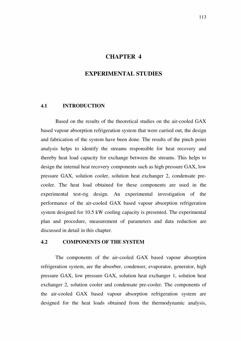
Solution Heat
Exchanger 2
(Figure 4.8)
Weak solution inlet temperature: 102°C
Weak solution outlet temperature: 112°C
Strong solution inlet temperature: 130°C
Strong solution outlet temperature: 120 °C
Mass flow rate of weak solution: 0.058 kg/s
Mass flow rate of strong solution: 0.048 kg/s
Type: Tube-in-Tube
Material: Mild steel
Inner Tube diameter (ID): 62.7 mm
Thickness: 10.3 mm
Tube Length: 1210 mm
Outer Tube diameter (ID): 203 mm
Thickness: 16 mm
Tube Length: 1210 mm
Heat Transfer Duty: 3.57 kW
Heat Transfer Area: 0.10 m2
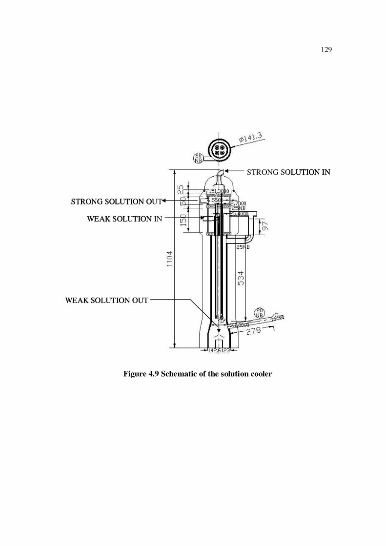
Component Design Conditions Specifications
Solution
Cooler
(Figure 4.9)
Weak solution inlet temperature: 112°C
Weak solution outlet temperature: 119°C
Strong solution inlet temperature: 150°C
Strong solution outlet temperature: 130 °C
Mass flow rate of weak solution: 0.058 kg/s
Mass flow rate of strong solution: 0.048 kg/s
Type: Shell and Tube
Material: Mild steel (Shell)
Mild Steel (Tube)
Shell Diameter (ID): 154.1 mm
Thickness: 14.2 mm
Shell Length: 1456 mm
Tube Diameter (ID): 10.2 mm
Thickness: 15.2 mm
Tube Length: 750 mm
Number of Tubes: 4
Heat Transfer Duty: 5.26 kW
Heat Transfer Area: 0.24 m2

120
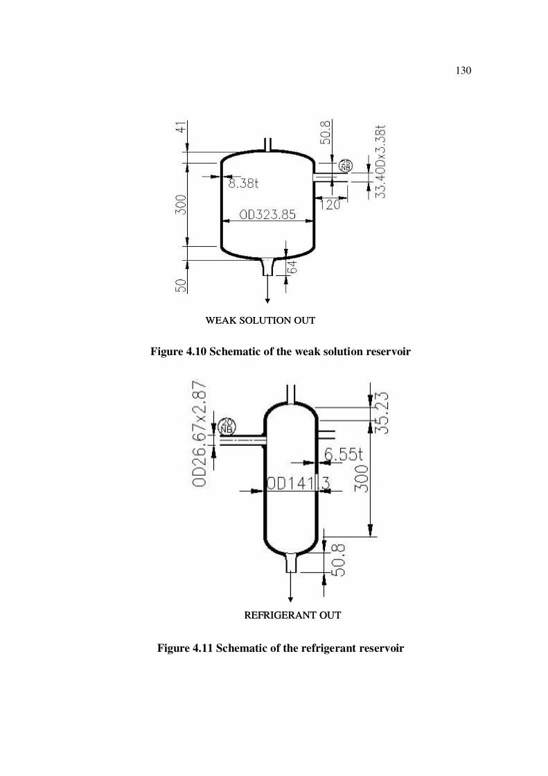
Table 4.2 (Concluded)
Component Specifications
Weak Solution
Reservoir
(Figure 4.10)
Type: Vertical Cylinder
Material: Mild steel
Diameter (ID): 307.1 mm; Thickness: 16.8 mm
Length: 385 mm
Component Specifications
Refrigerant Reservoir
(Figure 4.11)
Type: Vertical Cylinder
Material: Mild steel
Diameter (ID): 128.2 mm; Thickness: 13.1 mm
Length: 385 mm

121
LOW PRESSURE
REFRIGERANT
VAPOUR IN
HIGH PRESSURE
REFRIGERANT
VAPOUR IN
HIGH PRESSURE
REFRIGERANT
LIQUID OUT
WEAK
SOLUTION OUT
STRONG
SOLUTION IN
AIR IN
AIR OUT
LOW PRESSURE
REFRIGERANT
VAPOUR IN
HIGH PRESSURE
REFRIGERANT
VAPOUR IN
HIGH PRESSURE
REFRIGERANT
LIQUID OUT
WEAK
SOLUTION OUT
STRONG
SOLUTION IN
AIR IN
AIR OUT
Figure 4.1 Schematic of the absorber and the condensor

122
CHILLED
WATER OUT
REFRIGERANT IN
CHILLED WATER IN
REFRIGERANT OUT
CHILLED
WATER OUT
REFRIGERANT IN
CHILLED WATER IN
REFRIGERANT OUT
Figure 4.2 Schematic of the evaporator

123
STRONG
SOLUTION OUT
WEAK
SOLUTION IN
REFRIGERANT
VAPOUR OUT
STRONG
SOLUTION OUT
WEAK
SOLUTION IN
REFRIGERANT
VAPOUR OUT
Figure 4.3 Schematic of the generator

124
WEAK
SOLUTION IN
WEAK
SOLUTION OUT
REFRIGERANT VAPOUR IN
REFRIGERANT
VAPOUR OUT
WEAK
SOLUTION IN
WEAK
SOLUTION OUT
REFRIGERANT VAPOUR IN
REFRIGERANT
VAPOUR OUT
Figure 4.4 Schematic of the high pressure GAX

125
REFRIGERANT
VAPOUR IN
STRONG SOLUTION IN
STRONG
SOLUTION OUT
WEAK SOLUTION OUT
WEAK
SOLUTION IN
REFRIGERANT
VAPOUR IN
STRONG SOLUTION IN
STRONG
SOLUTION OUT
WEAK SOLUTION OUT
WEAK
SOLUTION IN
Figure 4.5 Schematic of the low pressure GAX
126
REFRIGERANT
LIQUID OUT
REFRIGERANT VAPOUR OUT
REFRIGERANT
LIQUID IN
REFRIGERANT VAPOUR IN
REFRIGERANT
LIQUID OUT
REFRIGERANT VAPOUR OUT
REFRIGERANT
LIQUID IN
REFRIGERANT VAPOUR IN
Figure 4.6 Schematic of the condensate pre-cooler

127
STRONG SOLUTION IN
WEAK
SOLUTION IN
WEAK
SOLUTION OUT
STRONG SOLUTION OUT
STRONG SOLUTION IN
WEAK
SOLUTION IN
WEAK
SOLUTION OUT
STRONG SOLUTION OUT
Figure 4.7 Schematic of the solution heat exchanger 1

128
WEAK
SOLUTION IN
WEAK
SOLUTION OUT
STRONG SOLUTION OUT
STRONG SOLUTION IN
FLUE GAS IN
FLUE GAS OUT
WEAK
SOLUTION IN
WEAK
SOLUTION OUT
STRONG SOLUTION OUT
STRONG SOLUTION IN
FLUE GAS IN
FLUE GAS OUT
Figure 4.8 Schematic of the solution heat exchanger 2
129
WEAK SOLUTION IN
WEAK SOLUTION OUT
STRONG SOLUTION OUT
STRONG SOLUTION IN
WEAK SOLUTION IN
WEAK SOLUTION OUT
STRONG SOLUTION OUT
STRONG SOLUTION IN
Figure 4.9 Schematic of the solution cooler
130
WEAK SOLUTION OUTWEAK SOLUTION OUT
Figure 4.10 Schematic of the weak solution reservoir
REFRIGERANT OUTREFRIGERANT OUT
Figure 4.11 Schematic of the refrigerant reservoir
131
SP
SC
SX1
G
SX2
LPGAX
HPGAXE
RRSR
CPC
FGO
FGI
A
C
B
PRV
EV
F
RFMSFM
PT
PT
2
1
3
4
5
6 7
8
9
10
11
12 13
14 15
16
1718
19
20
21
2223
24
WEAK SOLUTION
STRONG SOLUTION
REFRIGERANT
SP
SC
SX1
G
SX2
LPGAX
HPGAXE
RRSR
CPC
FGO
FGI
A
C
B
PRV
EV
F
RFMSFM
PT
PT
2
1
3
4
5
6 7
8
9
10
11
12 13
14 15
16
1718
19
20
21
2223
24
WEAK SOLUTION
STRONG SOLUTION
REFRIGERANT
LEGEND
A – Absorber FGO – Flue Gas Outlet SC- Solution Cooler E – Evaporator
B – Burner G - Generator SFM – Solution Flow Meter EV – Expansion Valve
C – Condensor HPGAX – High Pressure GAX SP – Solution Pump F – Fan
CPC – Condensate Pre-Cooler LPGAX – Low Pressure GAX SR – Solution Receiver FGI – Flue Gas Inlet
PRV – Pressure Reducing Valve SX1 – Solution Heat Exchanger 1 RFM – Refrigerant Flow Meter
PT – Pressure Transducer SX2 – Solution Heat Exchanger 2 RR – Refrigerant Reservoir
Figure 4.12 Schematic of the experimental set up

132
Figure 4.13 Pictorial view of the components of the experimental set up before insulation

133
Figure 4.14 Pictorial view of the experimental set up before insulation

134
Figure 4.15 Pictorial view of the components of the experimental set up after insulation

135
1 Absorber
2 Burner
3 Condenser
4 Condensate Pre-Cooler
5 Evaporator
6 Generator
7 High Pressure GAX
8 Low pressure GAX
9 Pressure Transducer
10 Refrigerant Flow Meter
11 Solution Cooler
12 Solution Heat Exchanger 1
13 Solution Heat Exchanger 2
14 Solution Pump
15 Weak Solution Reservoir
13
54
10
13
2
4
7
6
5
89
10
11
12
13
14
15
16
13
54
10
13
2
4
7
6
5
89
10
11
12
13
14
15
16
Figure 4.16 Pictorial front view of the experimental set up after insulation
136
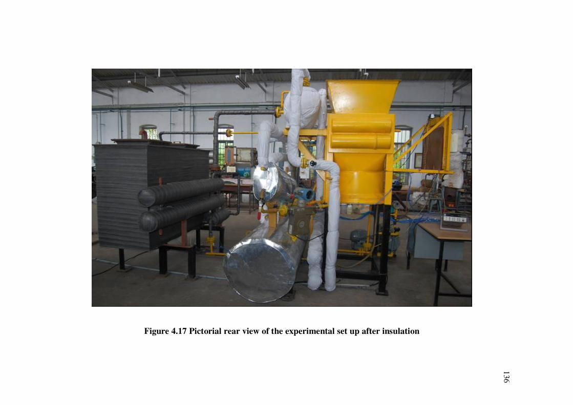
Figure 4.17 Pictorial rear view of the experimental set up after insulation
137
Power
Analyzer Data LoggerPower
Analyzer Data Logger
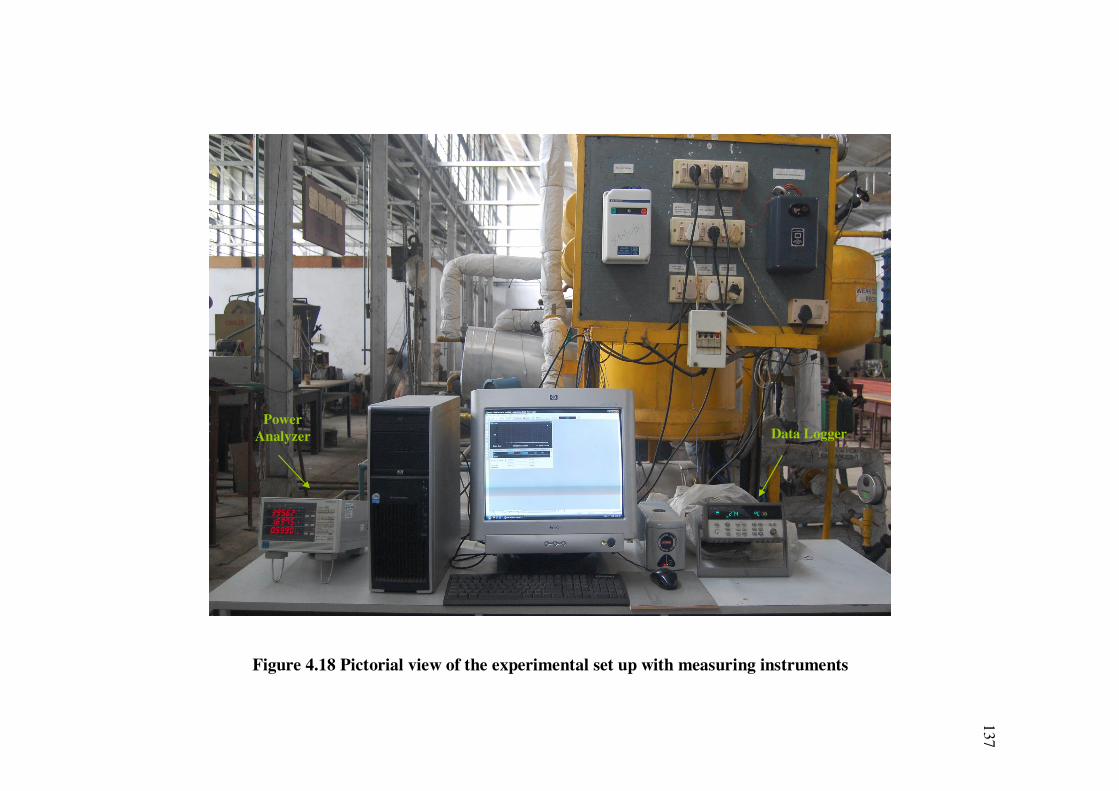
Figure 4.18 Pictorial view of the experimental set up with measuring instruments

138
The pictorial views of the components, and the experimental set up
before and after insulation are shown in Figures 4.13 to 4.18. The system has
two pressure levels. The absorber is at evaporator pressure and the generator
at condenser pressure. Weak solution (ws) is pumped by a 1.5 kW solution
pump (SP) of diaphragm type, from the absorber (A) to the high pressure
GAX (HPGAX). The HPGAX is an indirect counter current gas liquid heat
exchanger, which cools the refrigerant vapor (state point 16) coming from the
generator through the solution cooler (SC), by the incoming weak solution
entering the HPGAX at state point 2. The heat of rectification is thus
transferred to preheat the incoming weak solution. The weak solution enters
the low pressure GAX (LPGAX). The LPGAX absorbs a partial amount of
the refrigerant vapor (state point 24) from the condensate pre-cooler (CPC).
The simultaneous absorption of the refrigerant vapour takes place in both the
LPGAX and the absorber, due to the splitting of the refrigerant vapour at a
split factor of 0.8 to the absorber and the LPGAX. The pipe diameter from the
outlet of the condensate pre-cooler to the low pressure GAX, is reduced in
such a way that the refrigerant flow rate is at a split factor of 0.8 for a
diameter ratio of 1:2. Thus the split factor is maintained constant during
experiments and it is not measured. The heat of absorption, and the cooling of
strong solution from state point 12 to 13 are utilized to heat the weak solution
from state point 3 to 4, thus reducing the heat input. Then, the weak solution
enters the solution heat exchanger 1 (SX1). SX1 is the heat exchanger similar
to the one used in the conventional single effect system, where it exchanges
heat with the strong solution returning from the generator through the solution
heat exchanger 2 (SX2). It does not differ from SHX. The weak solution then
enters the solution heat exchanger 2 (SX2). In the SX2, the weak solution
(state point 5) is heated by both the strong solution (state point 9) and the
waste flue gases from the burner leaving the SX2. After extracting the energy
from the flue gas and the strong solution in the SX2, the weak solution finally
enters the generator through the Solution Cooler (SC), where it is further

139
heated by the strong solution leaving the generator. In the generator, the
external heat input from a diesel fired burner is supplied to generate the
refrigerant vapour. The purified vapor leaves the HPGAX and enters the
condenser at state point 17. Both the absorber and the condenser are air-
cooled. The air circulation is accomplished by a 0.75 kW fan.
The liquid refrigerant from the condenser enters the condensate pre-
cooler (CPC). The CPC is the economizer that is used in the system, which
heats the refrigerant vapour from the evaporator by sub-cooling the liquid
refrigerant from the condenser, before being throttled. The refrigerant vapour
from the CPC enters the absorber and the LPGAX. . Table 4.2 shows the type,
heat transfer area and the designed heat duty of the various components of the
air-cooled vapour absorption refrigeration system.
Table 4.3 Component details
S.No Component Type
Heat
Transfer
Area
(m2)
Heat Duty
(kW)
1 Absorber Finned 0.89 21.85
2 Condenser Finned 0.72 11.96
3 Evaporator Shell and Coil 5.77 10.5
4 Generator Direct Fired 1 23.27
5 High Pressure GAX Shell and Tube 2.98 3.65
6 Low Pressure GAX Shell and Tube 0.54 4.57
7 Condensate Pre-Cooler Shell and Tube 4.55 1.33
8 Solution Heat Exchanger 1 Tube-in-Tube 0.68 12.23
9 Solution Heat Exchanger 2 Tube-in-Tube 0.10 3.57
10 Solution Cooler Shell and Tube 0.24 5.26

140
4.4 CHARGING PROCEDURE
The individual components of the system are fabricated as per the
design specifications and subjected to hydraulic pressure testing upto 20 bar
to check for any leakage. Due to limited facility in the laboratory, the pressure
testing of the individual components was restricted upto 20 bar only The
pressure is maintained for a period of 2 to 3 days. The components are then
assembled and instrumented with pressure, temperature, and flow rate
measurements at the required location, as shown in Figure 4.12. The entire
system was again tested for leakage following the above procedure. The
system is then evacuated to an extent of 30 mm of Hg and the vacuum is
maintained for 3 days. To remove the non-condensable gases that may be
present, the system after evacuation is first charged with the refrigerant
vapour. The system is charged with calculated quantities of the refrigerant and
absorbent. The calculation procedure to determine the required quantity of
refrigerant and absorbent are given in Appendix 2 and the specifications of
the equipments such as the solution pump, absorber and condenser fan, burner
and power analyzer are given in Appendix 3.
4.5 MEASUREMENT OF PARAMETERS
The details of the instrumentation are presented in this section. The
parameters that are to be measured are the pressure, temperature, density and
mass flow rate of the solution, the air velocity, density and mass flow rate of
the refrigerant, and mass flow rate of the fuel. The uncertainty analysis of the
measured / calculated parameters is presented in Appendix 4.
4.5.1 Pressure
Pressure measurements are made by calibrated Pressure
Transducers. The low and high pressures in the system are measured with the
instrument ranging from 0 to 10 bar and 0 to 25 bar respectively, with an
uncertainty of ± 0.20%.

141
4.5.2 Temperature
Temperatures are measured with T type copper-constantan
thermocouples. The ends of all the thermocouples are connected to a data
acquisition system (Make: Agilent 34970A). The thermocouples were
calibrated at ice point of water and ambient temperature. Good agreement is
observed between the thermometer readings and measured readings of the
temperature using T-type thermocouples. The thermocouples are fixed at
various locations on the experimental set up. The measurements are made
with an uncertainty of ± 0.5oC. These data are stored in a data acquisition
system.
4.5.3 Flow Rate
The mass flow rate of the weak solution and the refrigerant are
measured by coriolis mass flow meters with an uncertainty of ± 0.2% and ±
0.15% respectively.
4.5.4 Concentration
The density and the temperature of both the weak solution and the
refrigerant are measured by coriolis mass flow meters. Using the correlation
which gives the relation between the specific volume, the temperature and the
concentration of the saturated ammonia-water solution, the concentration of
the weak solution and the refrigerant are determined as given below
3 3
0 0
( , ) j i
ij
i j
v T X a X T (4.1)
The coefficient of Equation (4.1) is taken from the ASHRAE
Handbook Fundamental (1993).

142
4.5.5 Fuel Consumption
The fuel flow rate to the generator is measured by a digital
weighing machine with an uncertainty of ± 0.05%.
4.5.6 Heat Loss
The heat loss from the surface of the generator to the surrounding is
calculated, based on the measurement of the temperatures at the generator
surface, insulation surface and the thermal conductivity of the insulation
material. The amount of heat loss from the generator to the surroundings is
estimated to be 0.175 kW, which is about 1.5% of the actual generator heat
input. The calculation procedure is mentioned in Appendix 5.
4.6 EXPERIMENTAL PLAN AND PROCEDURE
The following ranges of operating conditions are fixed for testing
the performance of the fabricated experimental setup.
(a) The mass flow rate of the weak solution is varied between
0.0248 kg/s and 0.0807 kg/s.
(b) The fuel flow rate to the generator is varied between 1kg/h
and 1.5 kg/h, by using different nozzles in the burner.
First, the absorber condenser fan is switched on, followed by the diesel
fired burner to supply heat input to the generator. The weak solution is then
circulated between the absorber and the generator, by switching on the
solution pump for the generation of the refrigerant vapour in the generator.
The condensing and evaporating temperatures varies with the cooling medium
and water temperatures respectively. The evaporating and condensing
temperatures were maintained by regulating the flow of strong solution and

143
the refrigerant using the pressure reducing valve and refrigerant expansion
valve.
The flow rates of the refrigerant, the pressure and temperature of
the components, air velocity, and fuel flow rate are noted periodically. After
the refrigerant reservoir is filled about 50%, the pressure reducing valve
between the condensate pre-cooler and the evaporator is adjusted in such a
way that a constant flow of liquid refrigerant is established. The level of the
weak solution in the weak solution reservoir in maintained constant for the
steady state operation, regulating the flow of the strong solution from the
generator to the absorber through the expansion valve. The refrigerant is also
maintained at a constant level in the refrigerant reservoir. When two to three
successive readings are almost the same, it can be concluded that the system
has attained the steady state.
As a safety precaution, since water has good affinity towards ammonia,
sufficient quantity of water has been kept as it can easily dilute the
concentration of the refrigerant. Safety face masks and gloves were also used
while operating the system. Any traces of ammonia leaked into the
atmosphere, can be easily detected before it reaches the toxic level due to its
pungent odour.
4.7 DATA PROCESSING
The circulation ratio (CR) is determined by the measured flow rate
of the weak solution and the refrigerant.
. .
ws rCR m / m (4.2)
144
The heat recovered by the internal heat recovery components is
estimated from the mass flow rate of the weak solution and the fluid
enthalpies.
The heat recovered by the high pressure GAX is
.
HPGAX ws 3 2Q m (h h ) (4.3)
The heat recovered by the low pressure GAX is
.
LPGAX ws 4 3Q m (h h ) (4.4)
The heat recovered by the solution heat exchanger 1 is
.
SX1 ws 5 4Q m (h h ) (4.5)
The heat recovered by the solution heat exchanger 2 is
.
SX2 ws 6 5Q m (h h ) (4.6)
The heat recovered by the solution cooler is
.
SC 7 7 6Q m (h h ) (4.7)
The heat recovered by the condensate pre cooler is
.
CPC 23 23 22Q m (h h ) (4.8)
In Equations (4.3) – (4.8), the temperatures were measured, using
calibrated copper-constantan thermocouples (T-type). To calculate the
enthalpy, the measured temperature and the solution concentration were used
in the correlation proposed by Sun (1997).
The heat rejected by the absorber and condensor is
.
AC a a ao aiQ m Cp (t t ) (4.9)
The measured temperatures were recorded in a data acquisition
system. The air velocity was measured by an anemometer at the inlet to the

145
absorber and condenser. The air flow rate is then calculated using the
following relation
.m a = (density of air) x (area) x (air velocity) (4.10)
The heat supplied to the generator is
.
fuel fuel fuelQ m (CV) (4.11)
CVfuel = 44,000 kJ/kg
Air-Fuel ratio = 14:1 (Ganesan 2002)
The cooling capacity is estimated by calculating the rate of heat
removal from a constant quantity of water.
Q m Cp dt / dw wE (4.12)
The volume of the evaporator shell is calculated and the required
quantity of water is filled in. The water temperature in the evaporator shell
was measured at three different locations (top, middle and bottom) using
copper-constantan thermocouples. The measurements were recorded and
stored periodically every 15 minutes. A graph between time and temperature
is plotted and the slope is taken for the calculation. The variation of ambient
air temperature during the course of experiment varies in the range of ± 3°C
only. This variation does not contribute significantly on the performance of
the system. The fuel COP is then determined using the relation
fu el E fu e lC O P Q Q (4.13)
The total COP is calculated considering the auxiliary power
required to operate the solution pump, fan and the burner.
total E fuel SP f bC O P Q (Q W W W ) (4.14)

146
The auxiliary powers were measured by using a calibrated digital
power analyzer.
4.8 RESULTS AND DISCUSSION
The performance of the system was evaluated by varying the mass
flow rate of the weak solution and the fuel flow rate to the generator.
4.8.1 Variation of the system pressures
Figure 4.19 shows the variation of the system pressures with time
for a constant weak solution and fuel flow rate and split factor. The split
factor is defined as the ratio of the mass flow rate of the refrigerant to the
absorber, to the total mass flow rate of the refrigerant in the cycle. The low
0
5
10
15
20
25
7.00 8.00 9.00 10.00 11.00 12.00 13.00 14.00 15.00 16.00 17.00
Condensor
Evaporator
Time (h)
Pres
sure
(ba
r)
Z = 0.8.
0.0578 /wsm kg s.
1.05 /fuelm kg h
0
5
10
15
20
25
7.00 8.00 9.00 10.00 11.00 12.00 13.00 14.00 15.00 16.00 17.00
Condensor
Evaporator
Time (h)
Pres
sure
(ba
r)
Z = 0.8.
0.0578 /wsm kg s.
1.05 /fuelm kg h
Figure 4.19 Variation of the system pressures with time
147
and high pressures stabilize at about 4 bar and 18 bar respectively, and the
system reaches the steady state in about 120 minutes of operation.
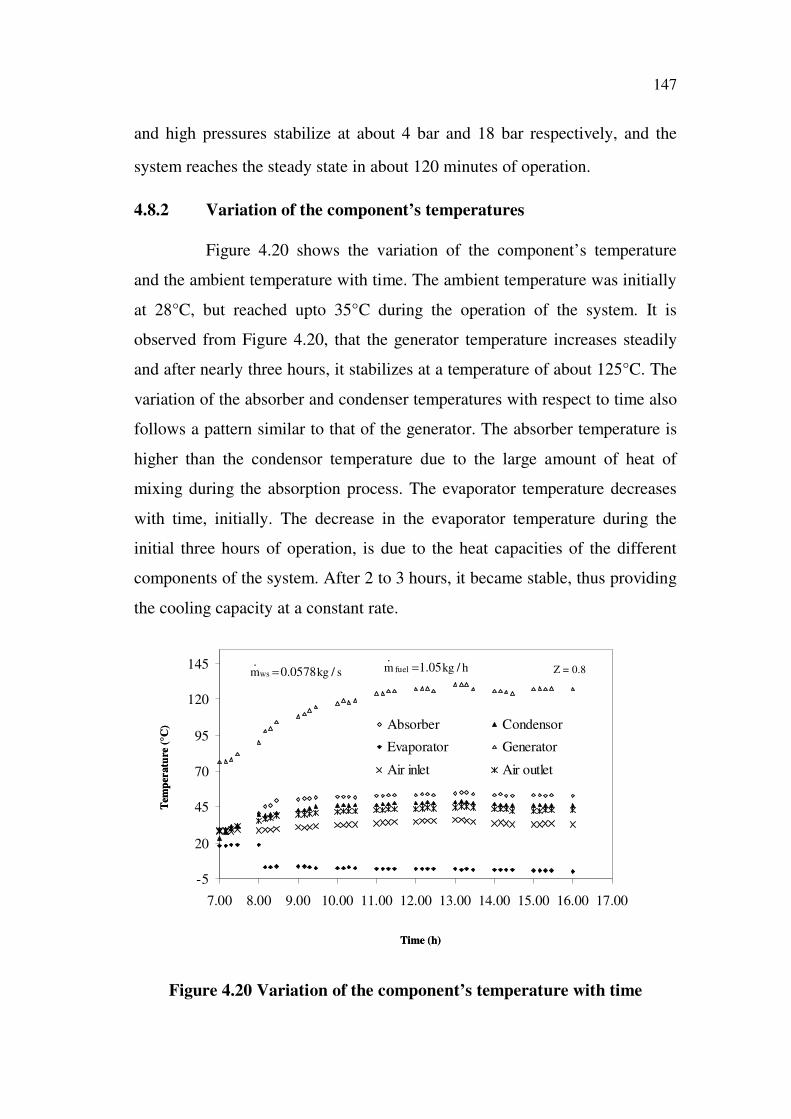
4.8.2 Variation of the component’s temperatures
Figure 4.20 shows the variation of the component’s temperature
and the ambient temperature with time. The ambient temperature was initially
at 28°C, but reached upto 35°C during the operation of the system. It is
observed from Figure 4.20, that the generator temperature increases steadily
and after nearly three hours, it stabilizes at a temperature of about 125°C. The
variation of the absorber and condenser temperatures with respect to time also
follows a pattern similar to that of the generator. The absorber temperature is
higher than the condensor temperature due to the large amount of heat of
mixing during the absorption process. The evaporator temperature decreases
with time, initially. The decrease in the evaporator temperature during the
initial three hours of operation, is due to the heat capacities of the different
components of the system. After 2 to 3 hours, it became stable, thus providing
the cooling capacity at a constant rate.
Figure 4.20 Variation of the component’s temperature with time
-5
20
45
70
95
120
145
7.00 8.00 9.00 10.00 11.00 12.00 13.00 14.00 15.00 16.00 17.00
Absorber Condensor
Evaporator Generator
Air inlet Air outlet
Time (h)
Tem
per
atu
re (
°C)
Z = 0.8.
0.0578 /wsm kg s
.1.05 /fuelm kg h
-5
20
45
70
95
120
145
7.00 8.00 9.00 10.00 11.00 12.00 13.00 14.00 15.00 16.00 17.00
Absorber Condensor
Evaporator Generator
Air inlet Air outlet
Time (h)
Tem
per
atu
re (
°C)
Z = 0.8.
0.0578 /wsm kg s
.1.05 /fuelm kg h
148
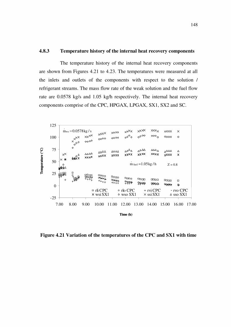
4.8.3 Temperature history of the internal heat recovery components
The temperature history of the internal heat recovery components
are shown from Figures 4.21 to 4.23. The temperatures were measured at all
the inlets and outlets of the components with respect to the solution /
refrigerant streams. The mass flow rate of the weak solution and the fuel flow
rate are 0.0578 kg/s and 1.05 kg/h respectively. The internal heat recovery
components comprise of the CPC, HPGAX, LPGAX, SX1, SX2 and SC.
Figure 4.21 Variation of the temperatures of the CPC and SX1 with time
-25
0
25
50
75
100
125
7.00 8.00 9.00 10.00 11.00 12.00 13.00 14.00 15.00 16.00 17.00
rli CPC rlo CPC rvi CPC rvo CPCwsi SX1 wso SX1 ssi SX1 sso SX1
Time (h)
Tem
per
atu
re (
°C)
Z = 0.8
.0.0578 /wsm kg s
.1.05 /fuelm kg h
-25
0
25
50
75
100
125
7.00 8.00 9.00 10.00 11.00 12.00 13.00 14.00 15.00 16.00 17.00
rli CPC rlo CPC rvi CPC rvo CPCwsi SX1 wso SX1 ssi SX1 sso SX1
Time (h)
Tem
per
atu
re (
°C)
Z = 0.8
.0.0578 /wsm kg s
.1.05 /fuelm kg h

149
Figure 4.22 Variation of the temperatures of the LPGAX and SX2 with
time
0
25
50
75
100
125
7.00 8.00 9.00 10.00 11.00 12.00 13.00 14.00 15.00 16.00 17.00
wsi HPGAX wso HPGAX rvi HPGAXrvo HPGAX wsi SC wso SCssi SC sso SC
Time (h)
Tem
pera
ture
(°C
) Z = 0.8
.0.0578 /wsm kg s
.1.05 /fuelm kg h
0
25
50
75
100
125
7.00 8.00 9.00 10.00 11.00 12.00 13.00 14.00 15.00 16.00 17.00
wsi HPGAX wso HPGAX rvi HPGAXrvo HPGAX wsi SC wso SCssi SC sso SC
Time (h)
Tem
pera
ture
(°C
) Z = 0.8
.0.0578 /wsm kg s
.1.05 /fuelm kg h
Figure 4.23 Variation of the temperatures of the HPGAX and SC with
time
Tem
pera
ture
(°C
)
-25
0
25
50
75
100
125
7.00 8.00 9.00 10.00 11.00 12.00 13.00 14.00 15.00 16.00 17.00
wsi LPGAX wso LPGAX ssi LPGAX sso LPGAX rvi LPGAX
wsi SX2 wso SX2 ssi SX2 sso SX2
Time (h)
Tem
pera
ture
(°C
)
-25
0
25
50
75
100
125
7.00 8.00 9.00 10.00 11.00 12.00 13.00 14.00 15.00 16.00 17.00
wsi LPGAX wso LPGAX ssi LPGAX sso LPGAX rvi LPGAX
wsi SX2 wso SX2 ssi SX2 sso SX2
Time (h)

150
The rise in the temperature of the weak solution is about 5 to 10 °C
in the GAX component, namely, the HPGAX and LPGAX, and also in the
SC, whereas it is about 5°C in the SX2. The SX1 accounts for nearly 25 to 30
°C rise in the amount of heat gained by the weak solution. The effectiveness
of the SX1 is determined to be 80 to 85%.
4.8.4 Circulation ratio and weight fraction
The variation of the circulation ratio and the weight fraction, with
respect to time for a typical operating condition is shown in Figure 4.24. The
circulation ratio has a greater impact on the system performance. The
circulation ratio was initially high, because of the less amount of refrigerant
circulation, and it became steady after 2 hours from the starting time of the
system operation. The weight fraction of the weak solution is high initially,
mainly due to the refrigerant that was ‘emptied’ out of the refrigerant circuit
and ‘stored’ in the solution after the previous run. The weight fraction of the
pure refrigerant remains almost constant from the starting time of the
refrigerant circulation. The refrigerant vapour leaving the HPGAX is
condensed in the condensor and is stored in the refrigerant reservoir.
Time (h)
CR
Wei
gh
t F
racti
on
(%
)
0
3
6
9
12
15
7.00 8.00 9.00 10.00 11.00 12.00 13.00 14.00 15.00 16.00 17.00
0
20
40
60
80
100
Xr
Xws Xss
Z = 0.8
CR
.0.0578 /wsm kg s
.1.05 /fuelm kg h
Time (h)
CR
Wei
gh
t F
racti
on
(%
)
0
3
6
9
12
15
7.00 8.00 9.00 10.00 11.00 12.00 13.00 14.00 15.00 16.00 17.00
0
20
40
60
80
100
Xr
Xws Xss
Z = 0.8
CR
.0.0578 /wsm kg s
.1.05 /fuelm kg h
Figure 4.24 Variation of the circulation ratio and weight fraction with
time

151
The concentration of the liquid refrigerant before it enters the evaporator
through the condensate pre-cooler, is estimated by using the correlation which
gives the relation between the specific volume, the temperature and the
concentration. The density and the temperature of the refrigerant is measured
by a coriolis mass flow meter. The HPGAX is very effective as the estimated
concentration of the refrigerant, was found to be 0.99, as inferred from Figure
4.24. The weight fraction of the strong solution also follows a trend similar to
that of the weak solution.
4.8.5 Pinch point diagram for a typical operating condition
The pinch point diagram for a typical operating condition is shown
in Figure 4.25. The heating process is represented by state points 2 to G. It
represents the amount of heat recovered by the weak solution in the various
internal heat recovery components. Processes 8 to A represent the cooling
process. The difference in the heat load between state points 2 and A, is the
absorber heat load. The difference in the heat load between state points 2 and
8 represents the total amount of heat recovered by the heat recovery
components. The amount of the external heat input that is supplied to the
generator is represented by the region between the state points 8 and G. The
pinch point is the closest approach temperature between the heating and cooling
curves. It can be inferred from the above figure that the pinch point occurs
between state points 4 and 11 on the heating and cooling curves respectively. A
pinch point of 7°C is obtained and a maximum cooling capacity of 9.5 kW is
attained. About 16 kW of internal heat has been recovered.The experimental
pinch point diagram which shows a pinch point of 7°C, has been plotted for a
particular operating condition of generator, absorber, condenser and
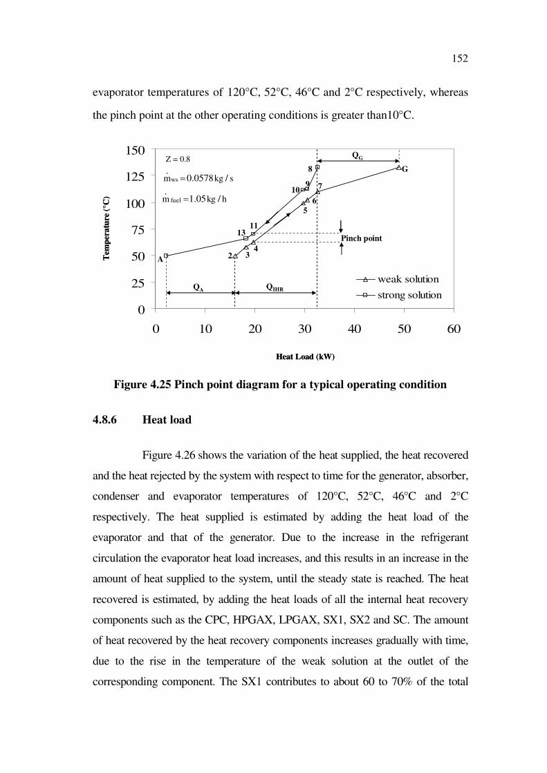
152
evaporator temperatures of 120°C, 52°C, 46°C and 2°C respectively, whereas
the pinch point at the other operating conditions is greater than10°C.
0
25
50
75
100
125
150
0 10 20 30 40 50 60
weak solution
strong solution
2 34
5
6
7
8
910
1113
G
A
QA
QG
QIHR
Pinch point
Z = 0.8
Heat Load (kW)
Tem
per
atu
re (
°C)
.0.0578 /wsm kg s
.1.05 /fuelm kg h
0
25
50
75
100
125
150
0 10 20 30 40 50 60
weak solution
strong solution
2 34
5
6
7
8
910
1113
G
A
QA
QG
QIHR
Pinch point
Z = 0.8
Heat Load (kW)
Tem
per
atu
re (
°C)
.0.0578 /wsm kg s
.1.05 /fuelm kg h
Figure 4.25 Pinch point diagram for a typical operating condition
4.8.6 Heat load
Figure 4.26 shows the variation of the heat supplied, the heat recovered
and the heat rejected by the system with respect to time for the generator, absorber,
condenser and evaporator temperatures of 120°C, 52°C, 46°C and 2°C
respectively. The heat supplied is estimated by adding the heat load of the
evaporator and that of the generator. Due to the increase in the refrigerant
circulation the evaporator heat load increases, and this results in an increase in the
amount of heat supplied to the system, until the steady state is reached. The heat
recovered is estimated, by adding the heat loads of all the internal heat recovery
components such as the CPC, HPGAX, LPGAX, SX1, SX2 and SC. The amount
of heat recovered by the heat recovery components increases gradually with time,
due to the rise in the temperature of the weak solution at the outlet of the
corresponding component. The SX1 contributes to about 60 to 70% of the total

153
amount of heat recovered internally. The internal heat recovered in the GAX
component and the SC is approximately 1.5 kW each.
Time (h)
Hea
t L
oad
(k
W)
10
15
20
25
7.00 8.00 9.00 10.00 11.00 12.00 13.00 14.00 15.00 16.00 17.00
Heat Supplied Heat Recovered Heat Rejected
tG = 120°C, tA = 52°C, tC = 46°C, tE = 2°C, Z = 0.8.
0.0578 /wsm kg s
.1.05 /fuelm kg h
Time (h)
Hea
t L
oad
(k
W)
10
15
20
25
7.00 8.00 9.00 10.00 11.00 12.00 13.00 14.00 15.00 16.00 17.00
Heat Supplied Heat Recovered Heat Rejected
tG = 120°C, tA = 52°C, tC = 46°C, tE = 2°C, Z = 0.8.
0.0578 /wsm kg s
.1.05 /fuelm kg h
Figure 4.26 Variation of the heat load with time
Overall, the heat recovery components provide nearly 16 kW of
heat recovered to the generator. The amount of heat rejected by the system is
the total amount of the heat rejected by both the absorber and the condenser.
The variation in the heat rejection load is not uniform, due to the variation in
the absorber and condenser load in different ambient conditions.
4.8.7 Cooling capacity and COP
The performance of the system in terms of the cooling capacity,
fuel and total COP, with respect to time is shown in Figure 4.27. The fuel
COP, calculated based on the fuel consumption rate and the rate of heat
removal from a fixed quantity of water, reached a maximum of 0.61 for the
generator, absorber, condenser and evaporator temperatures of 120°C, 52°C,
46°C and 2°C respectively.

154
CO
P
Cooli
ng C
ap
aci
ty (
kW
)
Time (h)
0.00
0.20
0.40
0.60
0.80
1.00
7.00 8.00 9.00 10.00 11.00 12.00 13.00 14.00 15.00 16.00 17.00
5
7
9
11
13
15
tE = 2°C tE = -2°C
COPfuel COPtotal Cooling Capacity
tG = 120°C, tA = 52°C, tC = 46°C.
0.0578 /wsm kg s.
1.05 /fuelm kg h
Z = 0.8
CO
P
Cooli
ng C
ap
aci
ty (
kW
)
Time (h)
0.00
0.20
0.40
0.60
0.80
1.00
7.00 8.00 9.00 10.00 11.00 12.00 13.00 14.00 15.00 16.00 17.00
5
7
9
11
13
15
tE = 2°C tE = -2°C
COPfuel COPtotal Cooling Capacity
tG = 120°C, tA = 52°C, tC = 46°C.
0.0578 /wsm kg s.
1.05 /fuelm kg h
Z = 0.8
Figure 4.27 Variation of the cooling capacity and the COP with time
The total COP, calculated by considering the parasitic power
consumption, reached a maximum of 0.58 for the same operating conditions,
which is about 8 % less than the fuel COP. The cooling capacity of the system
is about 7.4 kW and it remains almost constant. When the evaporator
temperature decreases from 2°C to -2°C while the other operating parameters
remain constant, the cooling capacity and the performance of the system are
reduced. This is because, when the evaporator temperature decreases, the
amount of the refrigerant mass flow rate decreases, and hence, the cooling
capacity and the COP of the system also decrease. The decrease in the actual
performance of the system, when the evaporator temperature varies from 2°C
to -2°C, is nearly 10 to 15%.

155
4.8.8 Experimental runs
Figure 4.28 depicts the performance of the system with respect to
the experimental runs. The mass flow rate of the weak solution is kept
constant at 0.0578 kg/s, and the fuel flow rate to the generator at 1.05 kg/h.
The system reached the maximum COP after 3 hours of operation during each
Figure 4.28 Variation of the COP with experimental runs
experimental run. The fuel and the total COP of the system vary between 0.60
and 0.63 and 0.56 and 0.59 respectively, for different experimental runs, for
the same operating conditions. The deviation between the thermodynamic and
fuel COP is estimated to be 20 to 25% due to heat losses and the internal
irreversibility in the system. For a particular set of experimental observations,
the performance parameters are given in Appendix 5. The efficiency of the
diesel fired burner is 95 to 98%. For calculation purposes, the efficiency is
taken as 100%.
CO
P
Experiment Runs
0.00
0.25
0.50
0.75
1.00
1 2 3 4 5 6 7 8 9 10 11 12 13 14 15 16 17 18 19 20 21 22 23 24 25
Fuel
Total
Thermodynamic
tG = 120°C, tA = 52°C, tC = 46°C, tE = 2°C, Z = 0.8
.0.0578 /ws sm kg
.1.05 /fuelm kg h
CO
P
Experiment Runs
0.00
0.25
0.50
0.75
1.00
1 2 3 4 5 6 7 8 9 10 11 12 13 14 15 16 17 18 19 20 21 22 23 24 25
Fuel
Total
Thermodynamic
tG = 120°C, tA = 52°C, tC = 46°C, tE = 2°C, Z = 0.8
.0.0578 /ws sm kg
.1.05 /fuelm kg h

156
4.8.9 Effect of fuel consumption
Figure 4.29 depicts the effect of the fuel flow rate in kg/h on the
cooling capacity and the fuel COP of the system, for an evaporator
temperature of 2°C. The mass flow rate of the weak solution is kept constant
at 0.0578 kg/s and the split factor at 0.8. It is inferred from the Figure that the
cooling capacity increases with an increase in the fuel flow rate. The increase
CO
P
Coo
lin
g C
ap
aci
ty (
kW
)
Fuel Consumption (kg/h)
0.40
0.60
0.80
1.00
1.00 1.10 1.20 1.30 1.40 1.50
5
6
7
8
9
10
Fuel COP
Cooling Capacity
tE = 2°C
Z = 0.8
.0.0578 /wsm kg s
CO
P
Coo
lin
g C
ap
aci
ty (
kW
)
Fuel Consumption (kg/h)
0.40
0.60
0.80
1.00
1.00 1.10 1.20 1.30 1.40 1.50
5
6
7
8
9
10
Fuel COP
Cooling Capacity
tE = 2°C
Z = 0.8
.0.0578 /wsm kg s
Figure 4.29 Variation of the cooling capacity and COP with the fuel
consumption
in the fuel flow rate increases the heat input to the generator, which leads to
the generation of more amount of refrigerant vapour, for a constant weak
solution flow rate. As a result of the increased refrigerant vapour generation,
the cooling capacity increases. However, the fuel COP of the system does not
increase because, firstly, the heat of generation increases as the generator
temperature increases. Secondly, the generator efficiency decreases with an
increasing fuel consumption rate. It is found that the fuel COP of 0.61 is
attained under the conditions analyzed for the fabricated system.

157
4.8.10 Influence of the sink temperatures on the circulation ratio
Figure 4.30 shows the variation of the circulation ratio with respect
to the sink temperature for the generator and evaporator temperatures of
120°C and 2°C respectively. For a constant weak solution flow rate, as the
Sink Temperature (°C)
CR
tG = 120°C, tE = 2°C
3.0
6.0
9.0
12.0
15.0
25 28 31 34 37 40
tG = 120°C, tE = 2°C.
0.0578 /wsm kg s
.1.05 /fuelm kg h
Z = 0.8
.1.40 /fuelm kg h
.1.25 /fuelm kg h
Sink Temperature (°C)
CR
tG = 120°C, tE = 2°C
3.0
6.0
9.0
12.0
15.0
25 28 31 34 37 40
tG = 120°C, tE = 2°C.
0.0578 /wsm kg s
.1.05 /fuelm kg h
Z = 0.8
.1.40 /fuelm kg h
.1.25 /fuelm kg h
Figure 4.30 Variation of the circulation ratio with the sink temperatures
sink temperature increases, the circulation ratio increases. This is because, as
the sink temperature increases the weak solution concentration decreases,
which results in a lower degassing width. The lower degassing width
increases the circulation ratio. For a constant sink temperature, the increase in
the fuel flow rate lowers the circulation ratio. This is due to the increase in the
refrigerant flow rate, for a constant weak solution rate.
4.8.11 Influence of the sink temperatures on the heat load
The variation of the heat supplied, heat recovered and heat rejected
with the sink temperatures is shown in Figure 4.31. The heat supplied is the
summation of the evaporator and generator load and the heat rejected is the

158
summation of the absorber and condenser heat load. The heat recovered by
the system is the total heat load of all the internal heat recovery components,
such as the high pressure GAX, the low pressure GAX, solution heat
exchangers 1 and 2, solution cooler and the condensate pre-cooler. As the sink
temperature increases, the total heat supplied reduces, due to the decrease in
the evaporator load at higher sink temperatures. The heat rejected from the
system also decreases with the sink temperature. However, the heat recovered
by the system increases due to the increase in the temperature difference
across the internal heat recovery components. The reason for large difference
between the heat supplied to the system and the heat rejected by the system as
inferred from the Figures 4.26 and 4.31 is because, the heat loss from the
other components and the connecting pipelines were not measured.
Sink Temperature (°C)
Hea
t L
oa
d (
kW
)
5
10
15
20
25
25 28 31 34 37 40
Heat Supplied
Heat Recovered
Heat Rejected
tG = 120°C, tE = 2°C.
0.0578 /wsm kg s.
1.05 /fuelm kg h
Sink Temperature (°C)
Hea
t L
oa
d (
kW
)
5
10
15
20
25
25 28 31 34 37 40
Heat Supplied
Heat Recovered
Heat Rejected
tG = 120°C, tE = 2°C.
0.0578 /wsm kg s.
1.05 /fuelm kg h
Figure 4.31 Variation of the heat load with the sink temperatures
159
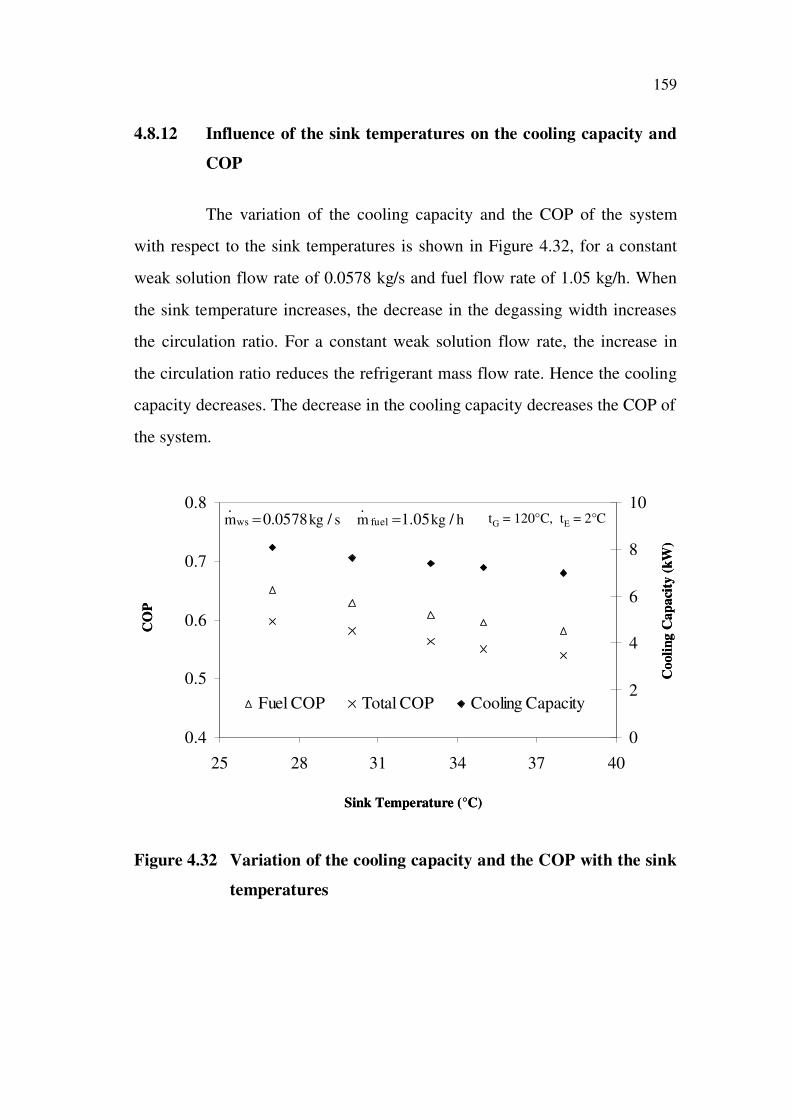
4.8.12 Influence of the sink temperatures on the cooling capacity and
COP
The variation of the cooling capacity and the COP of the system
with respect to the sink temperatures is shown in Figure 4.32, for a constant
weak solution flow rate of 0.0578 kg/s and fuel flow rate of 1.05 kg/h. When
the sink temperature increases, the decrease in the degassing width increases
the circulation ratio. For a constant weak solution flow rate, the increase in
the circulation ratio reduces the refrigerant mass flow rate. Hence the cooling
capacity decreases. The decrease in the cooling capacity decreases the COP of
the system.
Sink Temperature (°C)
CO
P
Co
oli
ng
Ca
pa
city
(k
W)
0.4
0.5
0.6
0.7
0.8
25 28 31 34 37 40
0
2
4
6
8
10
Fuel COP Total COP Cooling Capacity
.0.0578 /wsm kg s
.1.05 /fuelm kg h tG = 120°C, tE = 2°C
Sink Temperature (°C)
CO
P
Co
oli
ng
Ca
pa
city
(k
W)
0.4
0.5
0.6
0.7
0.8
25 28 31 34 37 40
0
2
4
6
8
10
Fuel COP Total COP Cooling Capacity
.0.0578 /wsm kg s
.1.05 /fuelm kg h tG = 120°C, tE = 2°C
Figure 4.32 Variation of the cooling capacity and the COP with the sink
temperatures

160
4.8.13 Second law efficiency
Figure 4.33 shows the variation of the second law efficiency with
respect to the sink temperatures, for a constant weak solution flow rate and
constant generator and evaporator temperatures. With increase in the sink
temperature, the fuel and the carnot COP decreases. Since the rate at which
the carnot COP decreases is higher that that of fuel COP, the second law
efficiency increases.
0.20
0.25
0.30
0.35
0.40
0.45
25 28 31 34 37 40
Sink Temperature (°C)
Sec
on
d l
aw
eff
icie
ncy
tG = 120°C, tE = 2°C.
0.0578 /wsm kg s.
1.05 /fuelm kg h
0.20
0.25
0.30
0.35
0.40
0.45
25 28 31 34 37 40
Sink Temperature (°C)
Sec
on
d l
aw
eff
icie
ncy
tG = 120°C, tE = 2°C.
0.0578 /wsm kg s.
1.05 /fuelm kg h
Figure 4.33 Variation of the second law efficiency with the sink
temperatures
4.9 ECONOMIC ANALYSIS
The incorporation of high pressure GAX, low pressure GAX,
solution cooler and the solution heat exchanger 2 increases the first cost of the
proposed system. Hence, it may not be economically viable when compared
to that of a simple system with only a solution heat exchanger and condensate
pre-cooler. However, for small and medium capacities up to 35 kW, air-

161
cooled systems are more economically viable compared to water-cooled
systems, due to large size of the cooling tower, installation problems etc.
Since the water cooled systems need a cooling tower, cooling
water pump etc, the installation cost will be higher than that of an air-cooled
one, by 20 to 25%, for the same capacity. For a conventional ammonia-water
system, the COP is about 0.5 and in the GAX system it is about 0.61, at a
generator, absorber, condenser, evaporator temperatures of 120°C, 52°C,
46°C, 2°C respectively. The amount of internal heat recovery is about 30 to
40 % more than in the conventional one, which would reduce the operating
costs by about 20%.
4.10 CONCLUSION
In this chapter, the design of the components of the air-cooled GAX
based vapour absorption refrigeration system, the working fluid charging
procedure, the measurement of parameters, and the experimental plan and
procedure have been presented. The results of the experimental investigations
on the air-cooled GAX based vapour absorption refrigeration system are
discussed. The influence of the various parameters such as the sink
temperature and the fuel flow rate on the performance of the system is also
discussed. The performance parameters studied are the circulation ratio,
internal heat recovered and the coefficient of performance. The conclusions
drawn from the experimental investigations are presented in the next chapter.


![cohort sep 2011.ppt [Kompatibilitetstilstand]publicifsv.sund.ku.dk/~pka/epiE11/coh-SF.pdf · Non-experimental studies No studies Non-experimental studies Sampling according exposure](https://img.pdfslide.net/doc/110x75/604672f5474efe54d3574c94/cohort-sep-2011ppt-kompatibilitetstilstand-pkaepie11coh-sfpdf-non-experimental.jpg)