Chapter 4: Exponential and Logarithmic Functions · 2015-02-02 · Chapter 4: Exponential and Logarithmic Functions Section 4.1 Exponential Functions ... 216 Chapter 4 Notice that

This chapter is part of Precalculus: An Investigation of Functions © Lippman & Rasmussen 2011. This material is licensed under a Creative Commons CC-BY-SA license.

Chapter 4: Exponential and Logarithmic Functions Section 4.1 Exponential Functions ............................................................................. 215 Section 4.2 Graphs of Exponential Functions............................................................. 232 Section 4.3 Logarithmic Functions ............................................................................. 242 Section 4.4 Logarithmic Properties............................................................................. 253 Section 4.5 Graphs of Logarithmic Functions ............................................................ 262 Section 4.6 Exponential and Logarithmic Models ...................................................... 270 Section 4.7 Fitting Exponentials to Data .................................................................... 289

Section 4.1 Exponential Functions India is the second most populous country in the world, with a population in 2008 of about 1.14 billion people. The population is growing by about 1.34% each year1. We might ask if we can find a formula to model the population, P, as a function of time, t, in years after 2008, if the population continues to grow at this rate. In linear growth, we had a constant rate of change – a constant number that the output increased for each increase in input. For example, in the equation 43)( += xxf , the slope tells us the output increases by three each time the input increases by one. This population scenario is different – we have a percent rate of change rather than a constant number of people as our rate of change. To see the significance of this difference consider these two companies: Company A has 100 stores, and expands by opening 50 new stores a year Company B has 100 stores, and expands by increasing the number of stores by 50% of their total each year. Looking at a few years of growth for these companies:

Year Stores, company A Stores, company B 0 100 Starting with 100 each

100

1 100 + 50 = 150 They both grow by 50 stores in the first year.

100 + 50% of 100 100 + 0.50(100) = 150

2 150 + 50 = 200 Store A grows by 50, Store B grows by 75

150 + 50% of 150 150 + 0.50(150) = 225

3 200 + 50 = 250 Store A grows by 50, Store B grows by 112.5

225 + 50% of 225 225 + 0.50(225) = 337.5

1 World Bank, World Development Indicators, as reported on http://www.google.com/publicdata, retrieved August 20, 2010

http://www.google.com/publicdata

Chapter 4 216

Notice that with the percent growth, each year the company is grows by 50% of the current year’s total, so as the company grows larger, the number of stores added in a year grows as well. To try to simplify the calculations, notice that after 1 year the number of stores for company B was:

)100(50.0100 + or equivalently by factoring 150)50.01(100 =+

We can think of this as “the new number of stores is the original 100% plus another 50%”. After 2 years, the number of stores was:

)150(50.0150 + or equivalently by factoring )50.01(150 + now recall the 150 came from 100(1+0.50). Substituting that,

225)50.01(100)50.01)(50.01(100 2 =+=++ After 3 years, the number of stores was:

)225(50.0225 + or equivalently by factoring )50.01(225 + now recall the 225 came from 2)50.01(100 + . Substituting that,

5.337)50.01(100)50.01()50.01(100 32 =+=++ From this, we can generalize, noticing that to show a 50% increase, each year we multiply by a factor of (1+0.50), so after n years, our equation would be

nnB )50.01(100)( += In this equation, the 100 represented the initial quantity, and the 0.50 was the percent growth rate. Generalizing further, we arrive at the general form of exponential functions. Exponential Function

An exponential growth or decay function is a function that grows or shrinks at a constant percent growth rate. The equation can be written in the form

xraxf )1()( += or xabxf =)( where b = 1+r Where a is the initial or starting value of the function r is the percent growth or decay rate, written as a decimal b is the growth factor or growth multiplier. Since powers of negative numbers behave strangely, we limit b to positive values.

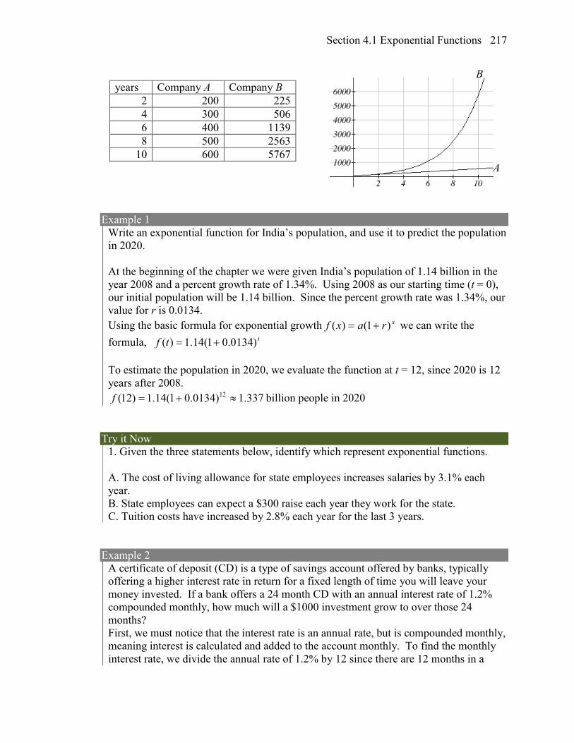
To see more clearly the difference between exponential and linear growth, compare the two tables and graphs below, which illustrate the growth of company A and B described above over a longer time frame if the growth patterns were to continue

Section 4.1 Exponential Functions 217

B years Company A Company B

2 200 225 4 300 506 6 400 1139 8 500 2563

10 600 5767 A Example 1

Write an exponential function for India’s population, and use it to predict the population in 2020. At the beginning of the chapter we were given India’s population of 1.14 billion in the year 2008 and a percent growth rate of 1.34%. Using 2008 as our starting time (t = 0), our initial population will be 1.14 billion. Since the percent growth rate was 1.34%, our value for r is 0.0134. Using the basic formula for exponential growth xraxf )1()( += we can write the formula, ttf )0134.01(14.1)( += To estimate the population in 2020, we evaluate the function at t = 12, since 2020 is 12 years after 2008.

337.1)0134.01(14.1)12( 12 ≈+=f billion people in 2020 Try it Now

1. Given the three statements below, identify which represent exponential functions. A. The cost of living allowance for state employees increases salaries by 3.1% each year. B. State employees can expect a $300 raise each year they work for the state. C. Tuition costs have increased by 2.8% each year for the last 3 years.

Example 2

A certificate of deposit (CD) is a type of savings account offered by banks, typically offering a higher interest rate in return for a fixed length of time you will leave your money invested. If a bank offers a 24 month CD with an annual interest rate of 1.2% compounded monthly, how much will a $1000 investment grow to over those 24 months? First, we must notice that the interest rate is an annual rate, but is compounded monthly, meaning interest is calculated and added to the account monthly. To find the monthly interest rate, we divide the annual rate of 1.2% by 12 since there are 12 months in a

Chapter 4 218

year: 1.2%/12 = 0.1%. Each month we will earn 0.1% interest. From this, we can set up an exponential function, with our initial amount of $1000 and a growth rate of r = 0.001, and our input m measured in months.

m

mf

+=

12012.11000)(

mmf )001.01(1000)( += After 24 months, the account will have grown to 24(24) 1000(1 0.001) $1024.28f = + =

Try it Now

2. Looking at these two equations that represent the balance in two different savings accounts, which account is growing faster, and which account will have a higher balance after 3 years?

( )ttA 05.11000)( = ( )ttB 075.1900)( = In all the preceding examples, we saw exponential growth. Exponential functions can also be used to model quantities that are decreasing at a constant percent rate. An example of this is radioactive decay, a process in which radioactive isotopes of certain atoms transform to an atom of a different type, causing a percentage decrease of the original material over time. Example 3

Bismuth-210 is an isotope that radioactively decays by about 13% each day, meaning 13% of the remaining Bismuth-210 transforms into another atom (polonium-210 in this case) each day. If you begin with 100 mg of Bismuth-210, how much remains after one week? With radioactive decay, instead of the quantity increasing at a percent rate, the quantity is decreasing at a percent rate. Our initial quantity is a = 100 mg, and our growth rate will be negative 13%, since we are decreasing: r = -0.13. This gives the equation:

dddQ )87.0(100)13.01(100)( =−= This can also be explained by recognizing that if 13% decays, then 87 % remains. After one week, 7 days, the quantity remaining would be

73.37)87.0(100)7( 7 ==Q mg of Bismuth-210 remains. Try it Now

3. A population of 1000 is decreasing 3% each year. Find the population in 30 years.


Example 4 T(q) represents the total number of Android smart phone contracts, in thousands, held by a certain Verizon store region measured quarterly since January 1, 2010, Interpret all of the parts of the equation 3056.231)64.1(86)2( 2 ==T . Interpreting this from the basic exponential form, we know that 86 is our initial value. This means that on Jan. 1, 2010 this region had 86,000 Android smart phone contracts. Since b = 1 + r = 1.64, we know that every quarter the number of smart phone contracts grows by 64%. T(2) = 231.3056 means that in the 2nd quarter (or at the end of the second quarter) there were approximately 231,305 Android smart phone contracts.

Finding Equations of Exponential Functions In the previous examples, we were able to write equations for exponential functions since we knew the initial quantity and the growth rate. If we do not know the growth rate, but instead know only some input and output pairs of values, we can still construct an exponential function. Example 5

In 2002, 80 deer were reintroduced into a wildlife refuge area from which the population had previously been hunted to elimination. By 2008, the population had grown to 180 deer. If this population grows exponentially, find a formula for the function. By defining our input variable to be t, years after 2002, the information listed can be written as two input-output pairs: (0,80) and (6,180). Notice that by choosing our input variable to be measured as years after the first year value provided, we have effectively “given” ourselves the initial value for the function: a = 80. This gives us an equation of the form

tbtf 80)( = . Substituting in our second input-output pair allows us to solve for b:

6180 80b= Divide by 80 6 180 9

80 4b = = Take the 6th root of both sides.

69 1.14474

b = =

This gives us our equation for the population: ttf )1447.1(80)( =

Recall that since b = 1+r, we can interpret this to mean that the population growth rate is r = 0.1447, and so the population is growing by about 14.47% each year.

In this example, you could also have used (9/4)^(1/6) to evaluate the 6th root if your calculator doesn’t have an nth root button.

Chapter 4 220

In the previous example, we chose to use the xabxf =)( form of the exponential function rather than the xraxf )1()( += form. This choice was entirely arbitrary – either form would be fine to use. When finding equations, the value for b or r will usually have to be rounded to be written easily. To preserve accuracy, it is important to not over-round these values. Typically, you want to be sure to preserve at least 3 significant digits in the growth rate. For example, if your value for b was 1.00317643, you would want to round this no further than to 1.00318. In the previous example, we were able to “give” ourselves the initial value by clever definition of our input variable. Next we consider a situation where we can’t do this. Example 6

Find a formula for an exponential function passing through the points (-2,6) and (2,1). Since we don’t have the initial value, we will take a general approach that will work for any function form with unknown parameters: we will substitute in both given input-output pairs in the function form xabxf =)( and solve for the unknown values, a and b. Substituting in (-2, 6) gives 26 −= ab Substituting in (2, 1) gives 21 ab= We now solve these as a system of equations. To do so, we could try a substitution approach, solving one equation for a variable, then substituting that expression into the second equation. Solving 26 −= ab for a:

22

6 6a bb−= =

In the second equation, 21 ab= , we substitute the expression above for a:

6389.061

61

61)6(1

4

4

4

22

≈=

=

=

=

b

b

bbb

Going back to the equation 26ba = lets us find a:

4492.2)6389.0(66 22 === ba Putting this together gives the equation xxf )6389.0(4492.2)( =


Try it Now 4. Given the two points (1, 3) and (2, 4.5) find the equation of an exponential function that passes through these two points.

Example 7

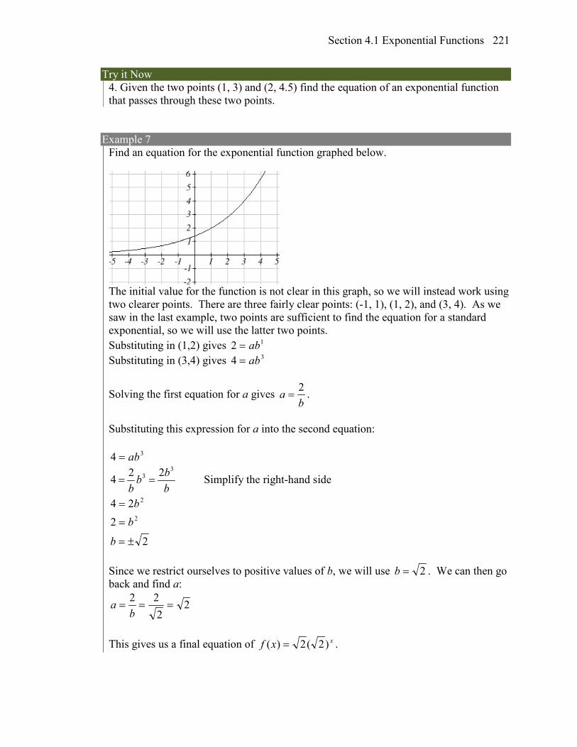
Find an equation for the exponential function graphed below.

The initial value for the function is not clear in this graph, so we will instead work using two clearer points. There are three fairly clear points: (-1, 1), (1, 2), and (3, 4). As we saw in the last example, two points are sufficient to find the equation for a standard exponential, so we will use the latter two points. Substituting in (1,2) gives 12 ab= Substituting in (3,4) gives 34 ab=

Solving the first equation for a gives b

a 2= .

Substituting this expression for a into the second equation:

34 ab=

bbb

b

33 224 == Simplify the right-hand side

2

224

2

2

±=

=

=

b

bb

Since we restrict ourselves to positive values of b, we will use 2=b . We can then go back and find a:

22

22===

ba

This gives us a final equation of xxf )2(2)( = .

Chapter 4 222

Compound Interest In the bank certificate of deposit (CD) example earlier in the section, we encountered compound interest. Typically bank accounts and other savings instruments in which earnings are reinvested, such as mutual funds and retirement accounts, utilize compound interest. The term compounding comes from the behavior that interest is earned not on the original value, but on the accumulated value of the account. In the example from earlier, the interest was compounded monthly, so we took the annual interest rate, usually called the nominal rate or annual percentage rate (APR) and divided by 12, the number of compounds in a year, to find the monthly interest. The exponent was then measured in months. Generalizing this, we can form a general formula for compound interest. If the APR is written in decimal form as r, and there are k compounding periods per year, then the interest per compounding period will be r/k. Likewise, if we are interested in the value after t years, then there will be kt compounding periods in that time. Compound Interest Formula

Compound Interest can be calculated using the formula kt

kratA

+= 1)(

Where A(t) is the account value t is measured in years a is the starting amount of the account, often called the principal r is the annual percentage rate (APR), also called the nominal rate k is the number of compounding periods in one year

Example 8

If you invest $3,000 in an investment account paying 3% interest compounded quarterly, how much will the account be worth in 10 years? Since we are starting with $3000, a = 3000 Our interest rate is 3%, so r = 0.03 Since we are compounding quarterly, we are compounding 4 times per year, so k = 4 We want to know the value of the account in 10 years, so we are looking for A(10), the value when t = 10.

05.4045$403.013000)10(

)10(4

=

+=A

The account will be worth $4045.05 in 10 years.


Example 9 A 529 plan is a college savings plan in which a relative can invest money to pay for a child’s later college tuition, and the account grows tax free. If Lily wants to set up a 529 account for her new granddaughter, wants the account to grow to $40,000 over 18 years, and she believes the account will earn 6% compounded semi-annually (twice a year), how much will Lily need to invest in the account now? Since the account is earning 6%, r = 0.06 Since interest is compounded twice a year, k = 2 In this problem, we don’t know how much we are starting with, so we will be solving for a, the initial amount needed. We do know we want the end amount to be $40,000, so we will be looking for the value of a so that A(18) = 40,000.

801,13$8983.2000,40

)8983.2(000,40206.01)18(000,40

)18(2

≈=

=

+==

a

a

aA

Lily will need to invest $13,801 to have $40,000 in 18 years.

Try it now

5. Recalculate example 2 from above with quarterly compounding. Because of compounding throughout the year, with compound interest the actual increase in a year is more than the annual percentage rate. If $1,000 were invested at 10%, the table below shows the value after 1 year at different compounding frequencies:

Frequency Value after 1 year Annually $1100 Semiannually $1102.50 Quarterly $1103.81 Monthly $1104.71 Daily $1105.16

If we were to compute the actual percentage increase for the daily compounding, there was an increase of $105.16 from an original amount of $1,000, for a percentage increase

of 10516.01000

16.105= = 10.516% increase. This quantity is called the annual percentage

yield (APY).

Chapter 4 224

Notice that given any starting amount, the amount after 1 year would be k

kraA

+= 1)1( . To find the total change, we would subtract the original amount, then

to find the percentage change we would divide that by the original amount:

111

−

+=

−

+ k

k

kr

a

akra

Annual Percentage Yield

The annual percentage yield is the actual percent a quantity increases in one year. It can be calculated as

11 −

+=

k

krAPY

Notice this is equivalent to finding the value of $1 after 1 year, and subtracting the original dollar. Example 10

Bank A offers an account paying 1.2% compounded quarterly. Bank B offers an account paying 1.1% compounded monthly. Which is offering a better rate? We can compare these rates using the annual percentage yield – the actual percent increase in a year.

Bank A: 012054.014012.01

4

=−

+=APY = 1.2054%

Bank B: 011056.0112011.01

12

=−

+=APY = 1.1056%

Bank B’s monthly compounding is not enough to catch up with Bank A’s better APR. Bank A offers a better rate.

A Limit to Compounding As we saw earlier, the amount we earn increases as we increase the compounding frequency. The table, though, shows that the increase from annual to semi-annual compounding is larger than the increase from monthly to daily compounding. This might lead us to believe that although increasing the frequency of compounding will increase our result, there is an upper limit to this process.


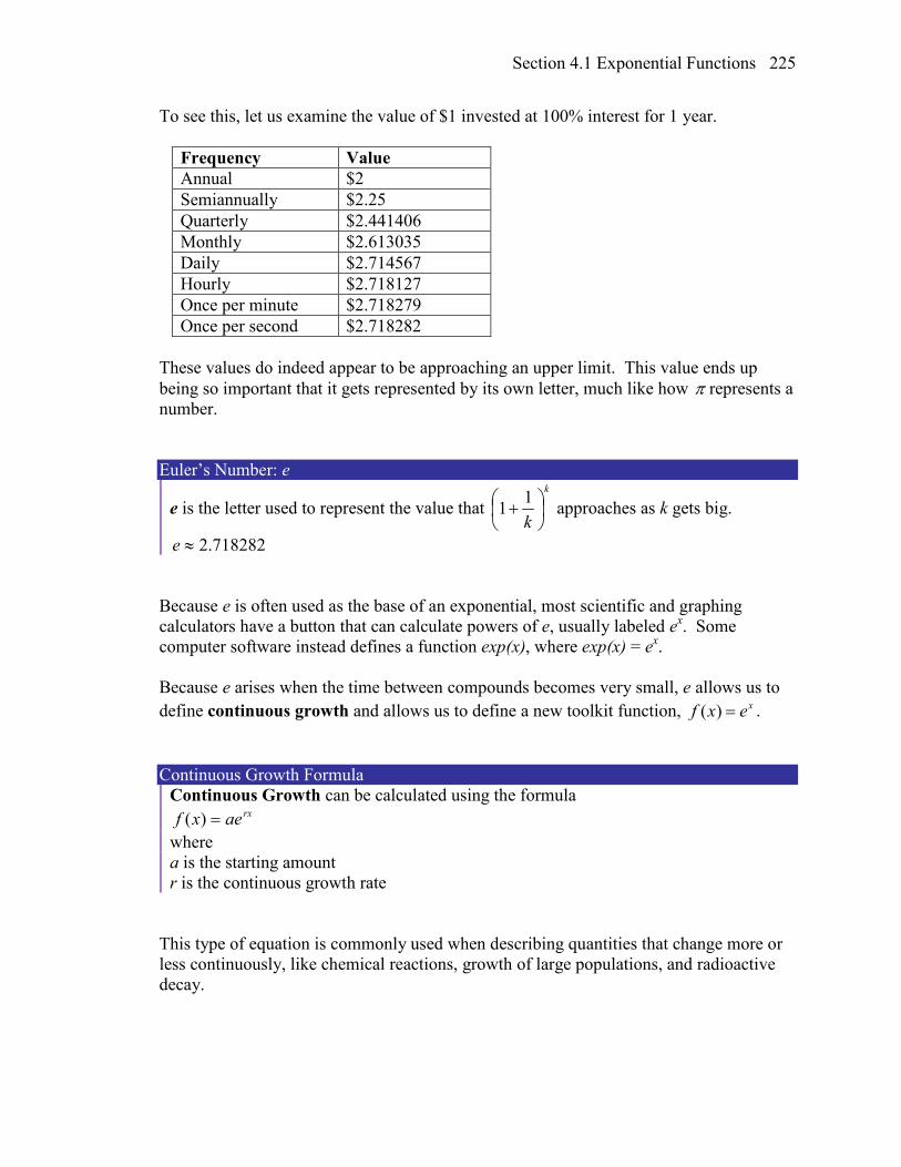
To see this, let us examine the value of $1 invested at 100% interest for 1 year.

Frequency Value Annual $2 Semiannually $2.25 Quarterly $2.441406 Monthly $2.613035 Daily $2.714567 Hourly $2.718127 Once per minute $2.718279 Once per second $2.718282

These values do indeed appear to be approaching an upper limit. This value ends up being so important that it gets represented by its own letter, much like how π represents a number. Euler’s Number: e

e is the letter used to represent the value that k

k

+

11 approaches as k gets big.

718282.2≈e Because e is often used as the base of an exponential, most scientific and graphing calculators have a button that can calculate powers of e, usually labeled ex. Some computer software instead defines a function exp(x), where exp(x) = ex. Because e arises when the time between compounds becomes very small, e allows us to define continuous growth and allows us to define a new toolkit function, ( ) xf x e= . Continuous Growth Formula

Continuous Growth can be calculated using the formula rxaexf =)(

where a is the starting amount r is the continuous growth rate

This type of equation is commonly used when describing quantities that change more or less continuously, like chemical reactions, growth of large populations, and radioactive decay.

Chapter 4 226

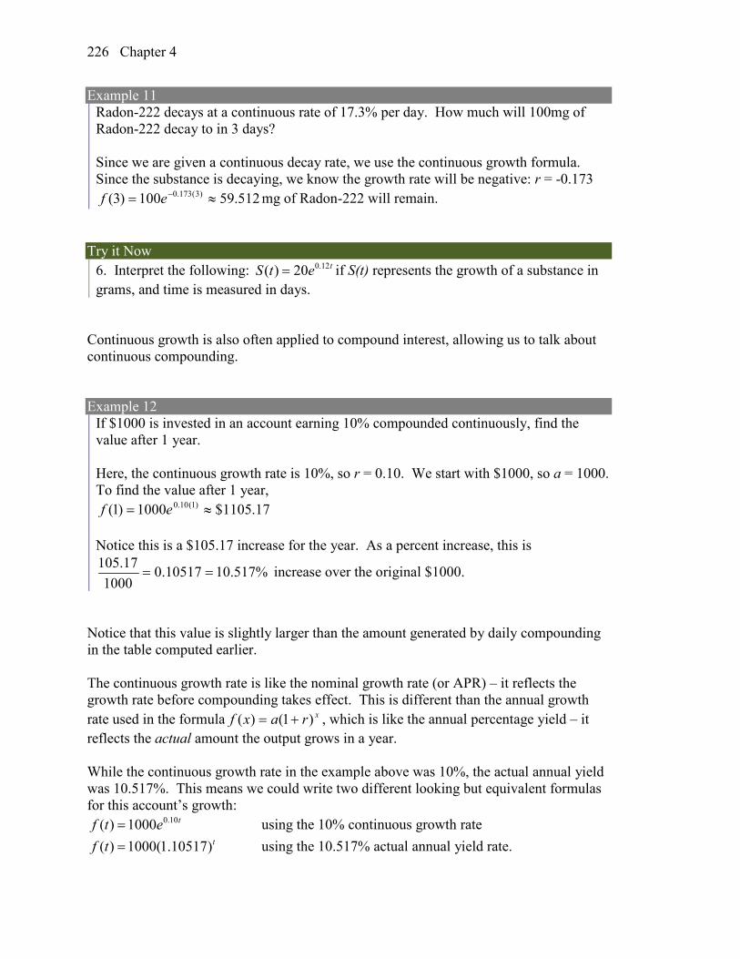
Example 11 Radon-222 decays at a continuous rate of 17.3% per day. How much will 100mg of Radon-222 decay to in 3 days? Since we are given a continuous decay rate, we use the continuous growth formula. Since the substance is decaying, we know the growth rate will be negative: r = -0.173

512.59100)3( )3(173.0 ≈= −ef mg of Radon-222 will remain. Try it Now

6. Interpret the following: 0.12( ) 20 tS t e= if S(t) represents the growth of a substance in grams, and time is measured in days.

Continuous growth is also often applied to compound interest, allowing us to talk about continuous compounding. Example 12

If $1000 is invested in an account earning 10% compounded continuously, find the value after 1 year. Here, the continuous growth rate is 10%, so r = 0.10. We start with $1000, so a = 1000. To find the value after 1 year,

17.1105$1000)1( )1(10.0 ≈= ef Notice this is a $105.17 increase for the year. As a percent increase, this is

%517.1010517.01000

17.105== increase over the original $1000.

Notice that this value is slightly larger than the amount generated by daily compounding in the table computed earlier. The continuous growth rate is like the nominal growth rate (or APR) – it reflects the growth rate before compounding takes effect. This is different than the annual growth rate used in the formula xraxf )1()( += , which is like the annual percentage yield – it reflects the actual amount the output grows in a year. While the continuous growth rate in the example above was 10%, the actual annual yield was 10.517%. This means we could write two different looking but equivalent formulas for this account’s growth:

0.10( ) 1000 tf t e= using the 10% continuous growth rate ( ) 1000(1.10517)tf t = using the 10.517% actual annual yield rate.


Important Topics of this Section Percent growth Exponential functions Finding formulas Interpreting equations Graphs Exponential Growth & Decay Compound interest Annual Percent Yield Continuous Growth

Try it Now Answers

1. A & C are exponential functions, they grow by a % not a constant number. 2. B(t) is growing faster, but after 3 years A(t) still has a higher account balance 3. 0071.401)97.0(1000 30 = 4. ( )xxf 5.12)( = 5. $1024.25 6. An initial substance weighing 20g is growing at a continuous rate of 12% per day.

Chapter 4 228

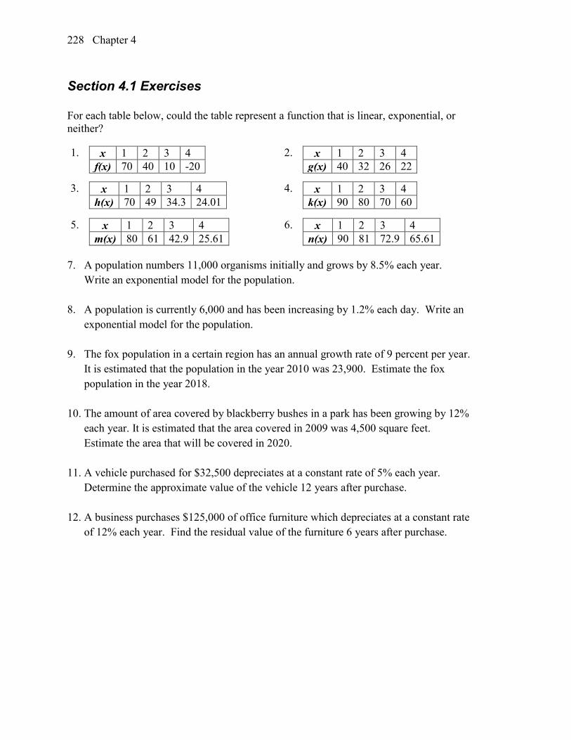
Section 4.1 Exercises For each table below, could the table represent a function that is linear, exponential, or neither?

1. x 1 2 3 4 f(x) 70 40 10 -20

2. x 1 2 3 4 g(x) 40 32 26 22

3. x 1 2 3 4 h(x) 70 49 34.3 24.01

4. x 1 2 3 4 k(x) 90 80 70 60

5. x 1 2 3 4 m(x) 80 61 42.9 25.61

6. x 1 2 3 4 n(x) 90 81 72.9 65.61

7. A population numbers 11,000 organisms initially and grows by 8.5% each year.

Write an exponential model for the population.

8. A population is currently 6,000 and has been increasing by 1.2% each day. Write an exponential model for the population.

9. The fox population in a certain region has an annual growth rate of 9 percent per year. It is estimated that the population in the year 2010 was 23,900. Estimate the fox population in the year 2018.

10. The amount of area covered by blackberry bushes in a park has been growing by 12% each year. It is estimated that the area covered in 2009 was 4,500 square feet. Estimate the area that will be covered in 2020.

11. A vehicle purchased for $32,500 depreciates at a constant rate of 5% each year. Determine the approximate value of the vehicle 12 years after purchase.

12. A business purchases $125,000 of office furniture which depreciates at a constant rate of 12% each year. Find the residual value of the furniture 6 years after purchase.


Find a formula for an exponential function passing through the two points. 13. ( )0, 6 , (3, 750) 14. ( )0, 3 , (2, 75)

15. ( )0, 2000 , (2, 20) 16. ( )0, 9000 , (3, 72)

17. ( )31, , 3, 242

−

18. ( )21, , 1,105

−

19. ( ) ( )2,6 , 3,1− 20. ( )3,4 , (3, 2)−

21. ( )3,1 , (5, 4) 22. ( )2,5 , (6, 9)

23. A radioactive substance decays exponentially. A scientist begins with 100 milligrams of a radioactive substance. After 35 hours, 50 mg of the substance remains. How many milligrams will remain after 54 hours?

24. A radioactive substance decays exponentially. A scientist begins with 110 milligrams of a radioactive substance. After 31 hours, 55 mg of the substance remains. How many milligrams will remain after 42 hours?

25. A house was valued at $110,000 in the year 1985. The value appreciated to $145,000 by the year 2005. What was the annual growth rate between 1985 and 2005? Assume that the house value continues to grow by the same percentage. What did the value equal in the year 2010?

26. An investment was valued at $11,000 in the year 1995. The value appreciated to $14,000 by the year 2008. What was the annual growth rate between 1995 and 2008? Assume that the value continues to grow by the same percentage. What did the value equal in the year 2012?

27. A car was valued at $38,000 in the year 2003. The value depreciated to $11,000 by the year 2009. Assume that the car value continues to drop by the same percentage. What will the value be in the year 2013?

28. A car was valued at $24,000 in the year 2006. The value depreciated to $20,000 by the year 2009. Assume that the car value continues to drop by the same percentage. What will the value be in the year 2014?

29. If $4,000 is invested in a bank account at an interest rate of 7 per cent per year, find the amount in the bank after 9 years if interest is compounded annually, quarterly, monthly, and continuously.

Chapter 4 230

30. If $6,000 is invested in a bank account at an interest rate of 9 per cent per year, find the amount in the bank after 5 years if interest is compounded annually, quarterly, monthly, and continuously.

31. Find the annual percentage yield (APY) for a savings account with annual percentage rate of 3% compounded quarterly.

32. Find the annual percentage yield (APY) for a savings account with annual percentage rate of 5% compounded monthly.

33. A population of bacteria is growing according to the equation 0.21 ( ) 1 600 tP t e= , with t measured in years. Estimate when the population will exceed 7569.

34. A population of bacteria is growing according to the equation 0.17 ( ) 1 200 tP t e= , with t measured in years. Estimate when the population will exceed 3443.

35. In 1968, the U.S. minimum wage was $1.60 per hour. In 1976, the minimum wage was $2.30 per hour. Assume the minimum wage grows according to an exponential model ( )w t , where t represents the time in years after 1960. [UW]

a. Find a formula for ( )w t . b. What does the model predict for the minimum wage in 1960? c. If the minimum wage was $5.15 in 1996, is this above, below or equal to what

the model predicts?

36. In 1989, research scientists published a model for predicting the cumulative number

of AIDS cases (in thousands) reported in the United States: ( )31980155

10ta t − =

,

where t is the year. This paper was considered a “relief”, since there was a fear the correct model would be of exponential type. Pick two data points predicted by the research model ( )a t to construct a new exponential model ( )b t for the number of cumulative AIDS cases. Discuss how the two models differ and explain the use of the word “relief.” [UW]


37. You have a chess board as pictured, with squares numbered 1 through 64. You also have a huge change jar with an unlimited number of dimes. On the first square you place one dime. On the second square you stack 2 dimes. Then you continue, always doubling the number from the previous square. [UW]

a. How many dimes will you have stacked on the 10th square?

b. How many dimes will you have stacked on the nth square?

c. How many dimes will you have stacked on the 64th square?

d. Assuming a dime is 1 mm thick, how high will this last pile be?

e. The distance from the earth to the sun is approximately 150 million km. Relate the height of the last pile of dimes to this distance.

Chapter 4 232

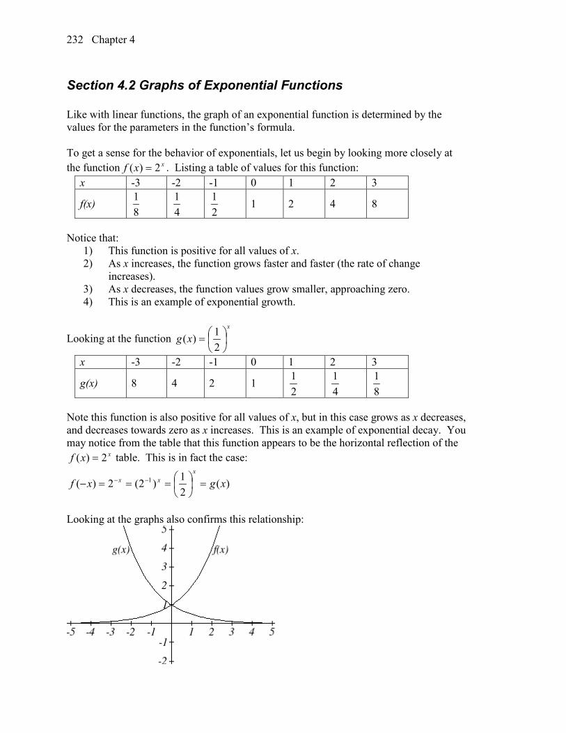
Section 4.2 Graphs of Exponential Functions Like with linear functions, the graph of an exponential function is determined by the values for the parameters in the function’s formula. To get a sense for the behavior of exponentials, let us begin by looking more closely at the function xxf 2)( = . Listing a table of values for this function:

x -3 -2 -1 0 1 2 3

f(x) 81

41

21 1 2 4 8

Notice that:

1) This function is positive for all values of x. 2) As x increases, the function grows faster and faster (the rate of change

increases). 3) As x decreases, the function values grow smaller, approaching zero. 4) This is an example of exponential growth.

Looking at the function x

xg

=

21)(

x -3 -2 -1 0 1 2 3

g(x) 8 4 2 1 21

41

81

Note this function is also positive for all values of x, but in this case grows as x decreases, and decreases towards zero as x increases. This is an example of exponential decay. You may notice from the table that this function appears to be the horizontal reflection of the

xxf 2)( = table. This is in fact the case:

)(21)2(2)( 1 xgxf

xxx =

===− −−

Looking at the graphs also confirms this relationship:

Section 4.2 Graphs of Exponential Functions 233

Consider a function for the form xabxf =)( . Since a, which we called the initial value in the last section, is the function value at an input of zero, a will give us the vertical intercept of the graph. From the graphs above, we can see that an exponential graph will have a horizontal asymptote on one side of the graph, and can either increase or decrease, depending upon the growth factor. This horizontal asymptote will also help us determine the long run behavior and is easy to determine from the graph. The graph will grow when the growth rate is positive, which will make the growth factor b larger than one. When it’s negative, the growth factor will be less than one. Graphical Features of Exponential Functions

Graphically, in the function xabxf =)( a is the vertical intercept of the graph b determines the rate at which the graph grows the function will increase if b > 1 the function will decrease if 0 < b < 1 The graph will have a horizontal asymptote at y = 0 The graph will be concave up if a > 0; concave down if a < 0. The domain of the function is all real numbers The range of the function is (0, )∞

When sketching the graph of an exponential function, it can be helpful to remember that the graph will pass through the points (0, a) and (1, ab). The value b will determine the function’s long run behavior: If b > 1, as ∞→x , ∞→)(xf and as −∞→x , 0)( →xf . If 0 < b < 1, as ∞→x , 0)( →xf and as −∞→x , ∞→)(xf . Example 1

Sketch a graph of x

xf

=

314)(

This graph will have a vertical intercept at (0,4), and

pass through the point

34,1 . Since b < 1, the graph

will be decreasing towards zero. Since a > 0, the graph will be concave up. We can also see from the graph the long run behavior: as ∞→x , 0)( →xf and as −∞→x , ∞→)(xf .

Chapter 4 234

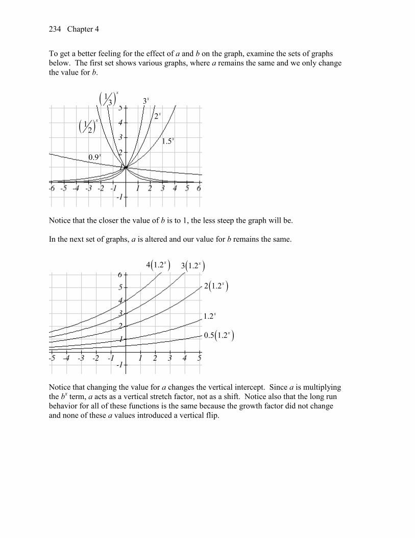
To get a better feeling for the effect of a and b on the graph, examine the sets of graphs below. The first set shows various graphs, where a remains the same and we only change the value for b.

Notice that the closer the value of b is to 1, the less steep the graph will be. In the next set of graphs, a is altered and our value for b remains the same.

Notice that changing the value for a changes the vertical intercept. Since a is multiplying the bx term, a acts as a vertical stretch factor, not as a shift. Notice also that the long run behavior for all of these functions is the same because the growth factor did not change and none of these a values introduced a vertical flip.

2x

1.5x

3x

0.9x

( )12

x

( )13

x

( )0.5 1.2x

1.2x

( )2 1.2x

( )3 1.2x ( )4 1.2x


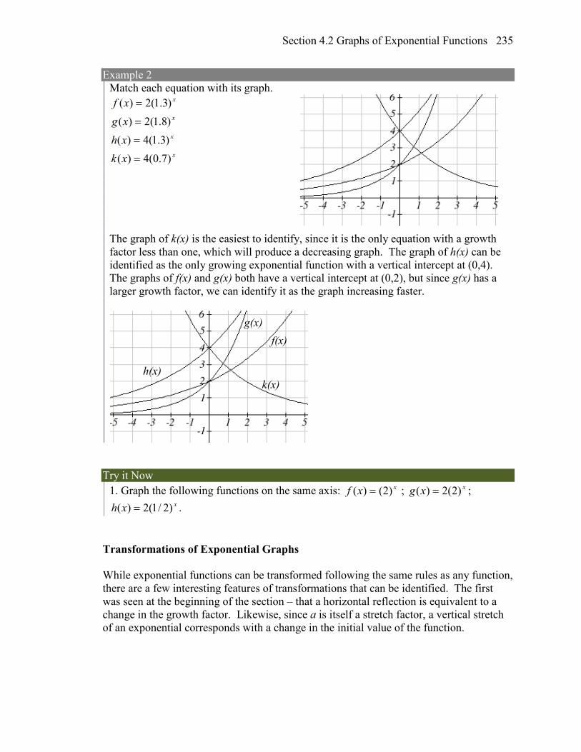
Example 2 Match each equation with its graph.

x

x

x

x

xkxhxgxf

)7.0(4)()3.1(4)()8.1(2)()3.1(2)(

=

=

=

=

The graph of k(x) is the easiest to identify, since it is the only equation with a growth factor less than one, which will produce a decreasing graph. The graph of h(x) can be identified as the only growing exponential function with a vertical intercept at (0,4). The graphs of f(x) and g(x) both have a vertical intercept at (0,2), but since g(x) has a larger growth factor, we can identify it as the graph increasing faster.

Try it Now

1. Graph the following functions on the same axis: xxf )2()( = ; xxg )2(2)( = ; xxh )2/1(2)( = .

Transformations of Exponential Graphs While exponential functions can be transformed following the same rules as any function, there are a few interesting features of transformations that can be identified. The first was seen at the beginning of the section – that a horizontal reflection is equivalent to a change in the growth factor. Likewise, since a is itself a stretch factor, a vertical stretch of an exponential corresponds with a change in the initial value of the function.

f(x) g(x)

h(x) k(x)

Chapter 4 236

Next consider the effect of a horizontal shift on an exponential function. Shifting the function xxf )2(3)( = four units to the left would give 4)2(3)4( +=+ xxf . Employing exponent rules, we could rewrite this:

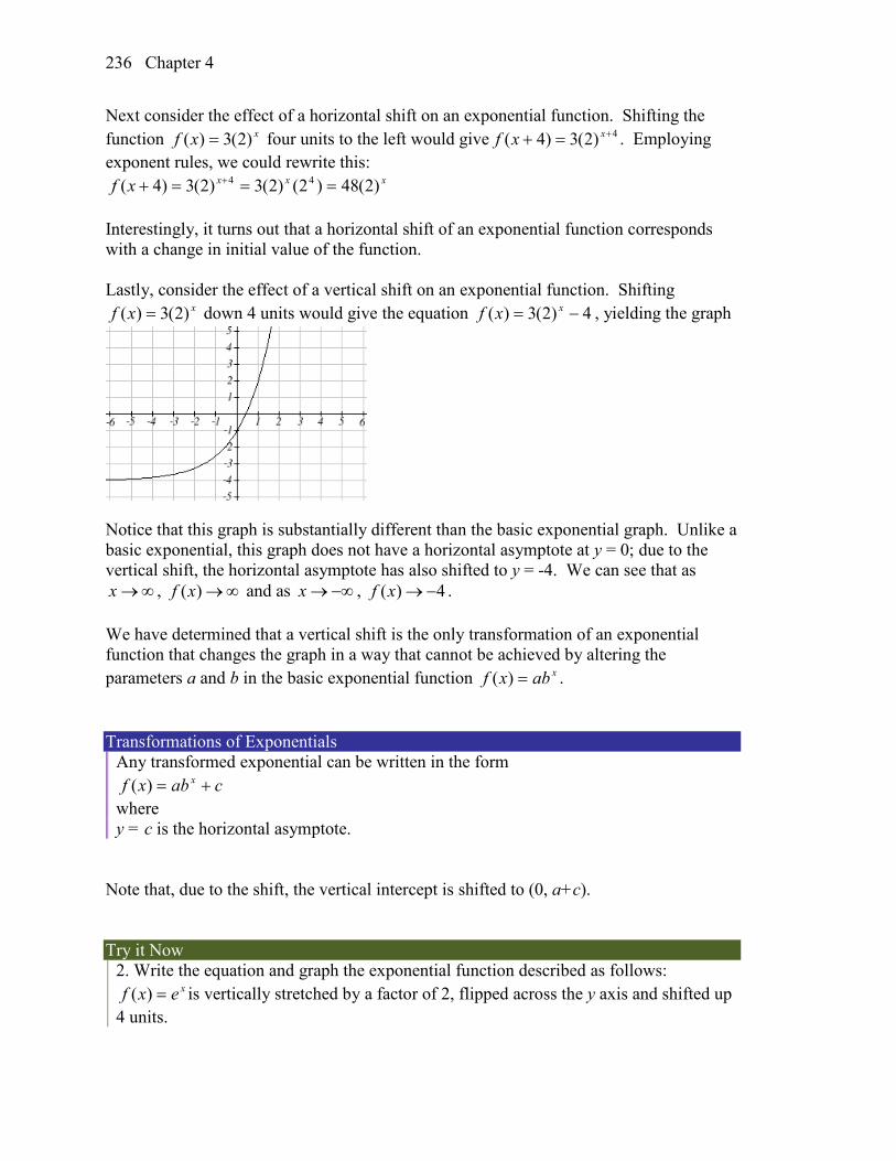
xxxxf )2(48)2()2(3)2(3)4( 44 ===+ + Interestingly, it turns out that a horizontal shift of an exponential function corresponds with a change in initial value of the function. Lastly, consider the effect of a vertical shift on an exponential function. Shifting

xxf )2(3)( = down 4 units would give the equation 4)2(3)( −= xxf , yielding the graph

Notice that this graph is substantially different than the basic exponential graph. Unlike a basic exponential, this graph does not have a horizontal asymptote at y = 0; due to the vertical shift, the horizontal asymptote has also shifted to y = -4. We can see that as x →∞ , ( )f x →∞ and as x →−∞ , ( ) 4f x →− . We have determined that a vertical shift is the only transformation of an exponential function that changes the graph in a way that cannot be achieved by altering the parameters a and b in the basic exponential function xabxf =)( . Transformations of Exponentials

Any transformed exponential can be written in the form cabxf x +=)(

where y = c is the horizontal asymptote.

Note that, due to the shift, the vertical intercept is shifted to (0, a+c). Try it Now

2. Write the equation and graph the exponential function described as follows: xexf =)( is vertically stretched by a factor of 2, flipped across the y axis and shifted up

4 units.


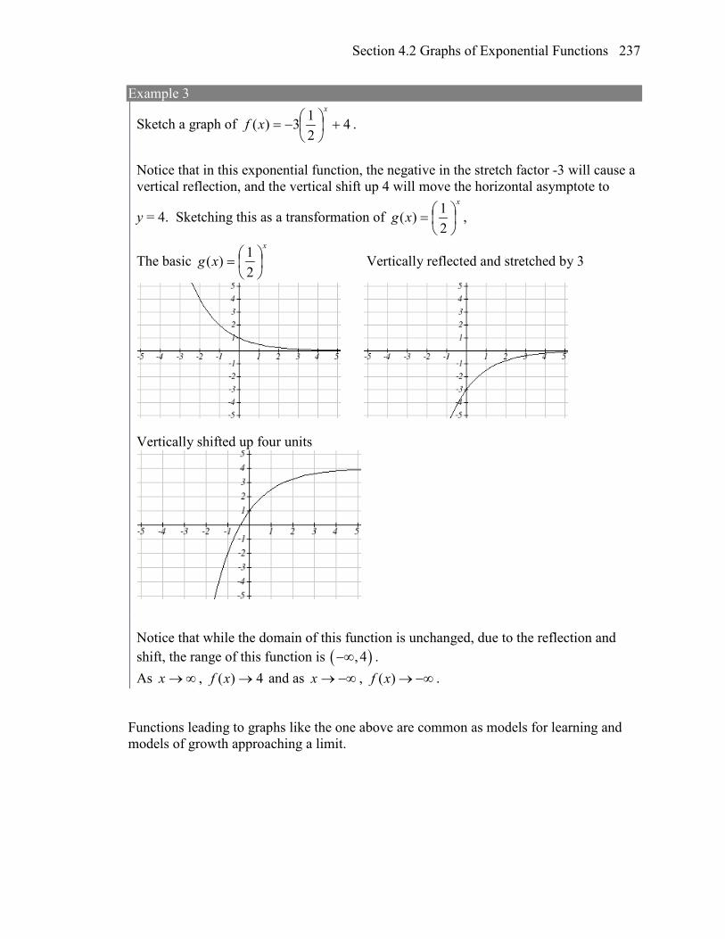
Example 3

Sketch a graph of 4213)( +

−=

x

xf .

Notice that in this exponential function, the negative in the stretch factor -3 will cause a vertical reflection, and the vertical shift up 4 will move the horizontal asymptote to

y = 4. Sketching this as a transformation of x

xg

=

21)( ,

The basic x

xg

=

21)( Vertically reflected and stretched by 3

Vertically shifted up four units

Notice that while the domain of this function is unchanged, due to the reflection and shift, the range of this function is ( ), 4−∞ . As ∞→x , 4)( →xf and as −∞→x , ( )f x →−∞ .

Functions leading to graphs like the one above are common as models for learning and models of growth approaching a limit.

Chapter 4 238

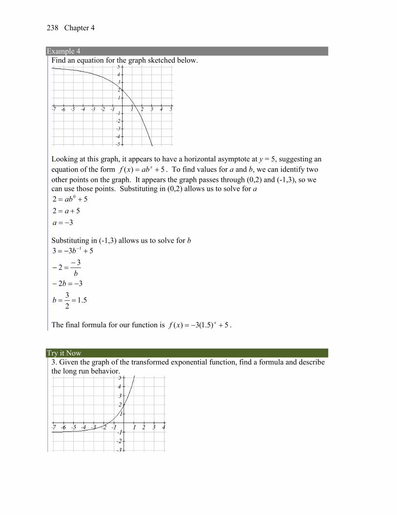
Example 4 Find an equation for the graph sketched below.

Looking at this graph, it appears to have a horizontal asymptote at y = 5, suggesting an equation of the form 5)( += xabxf . To find values for a and b, we can identify two other points on the graph. It appears the graph passes through (0,2) and (-1,3), so we can use those points. Substituting in (0,2) allows us to solve for a

352

52 0

−=+=+=

aaab

Substituting in (-1,3) allows us to solve for b

5.123

32

32

533 1

==

−=−

−=−

+−= −

b

bb

b

The final formula for our function is 5)5.1(3)( +−= xxf .

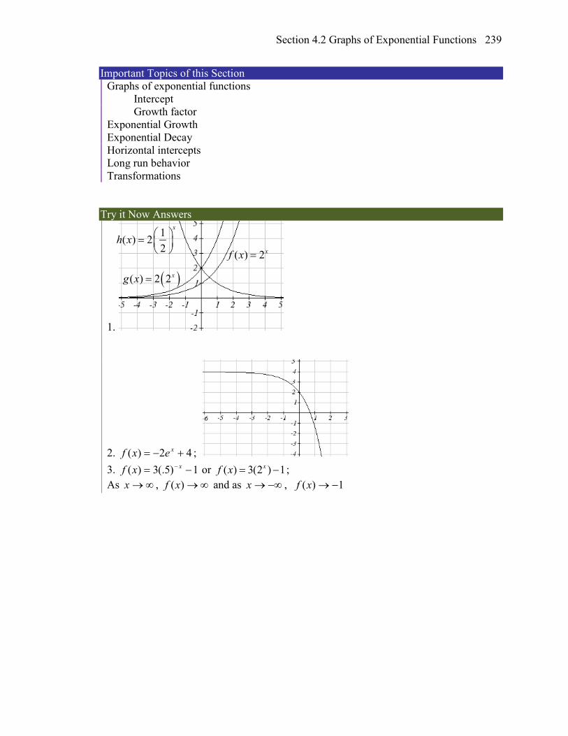
Try it Now

3. Given the graph of the transformed exponential function, find a formula and describe the long run behavior.


Important Topics of this Section Graphs of exponential functions Intercept Growth factor Exponential Growth Exponential Decay Horizontal intercepts Long run behavior Transformations

Try it Now Answers

1.

2. 42)( +−= xexf ; 3. 1)5(.3)( −= −xxf or ( ) 3(2 ) 1xf x = − ; As ∞→x , ∞→)(xf and as −∞→x , 1)( −→xf

( ) 2xf x =

( )( ) 2 2xg x =

1( ) 22

x

h x =

Chapter 4 240

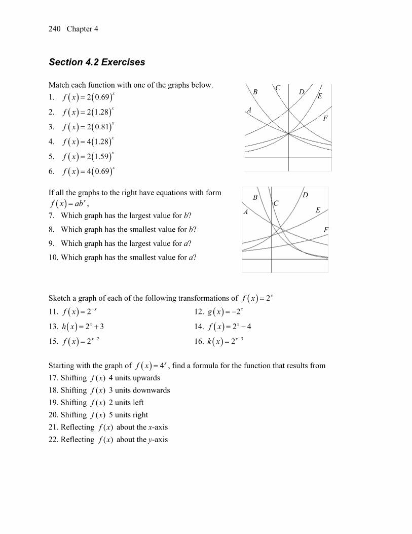
Section 4.2 Exercises Match each function with one of the graphs below. 1. ( ) ( )2 0.69 xf x =

2. ( ) ( )2 1.28 xf x =

3. ( ) ( )2 0.81 xf x =

4. ( ) ( )4 1.28 xf x =

5. ( ) ( )2 1.59 xf x =

6. ( ) ( )4 0.69 xf x = If all the graphs to the right have equations with form ( ) xf x ab= ,

7. Which graph has the largest value for b?

8. Which graph has the smallest value for b?

9. Which graph has the largest value for a?

10. Which graph has the smallest value for a?

Sketch a graph of each of the following transformations of ( ) 2xf x =

11. ( ) 2 xf x −= 12. ( ) 2xg x = −

13. ( ) 2 3xh x = + 14. ( ) 2 4xf x = −

15. ( ) 22xf x −= 16. ( ) 32xk x −=

Starting with the graph of ( ) 4xf x = , find a formula for the function that results from 17. Shifting ( )f x 4 units upwards 18. Shifting ( )f x 3 units downwards 19. Shifting ( )f x 2 units left 20. Shifting ( )f x 5 units right 21. Reflecting ( )f x about the x-axis 22. Reflecting ( )f x about the y-axis

A

B C D E

F

A

B C

D

E

F


Describe the long run behavior, as x →∞ and x →−∞ of each function 23. ( ) ( )5 4 1xf x = − − 24. ( ) ( )2 3 2xf x = − +

25. ( ) 13 22

x

f x = −

26. ( ) 14 14

x

f x = +

27. ( ) ( )3 4 2xf x −= + 28. ( ) ( )2 3 1xf x −= − − Find a formula for each function graphed as a transformation of ( ) 2xf x = .

29. 30.

31. 32. Find an equation for the exponential function graphed.

33. 34.

35. 36.

Chapter 4 242

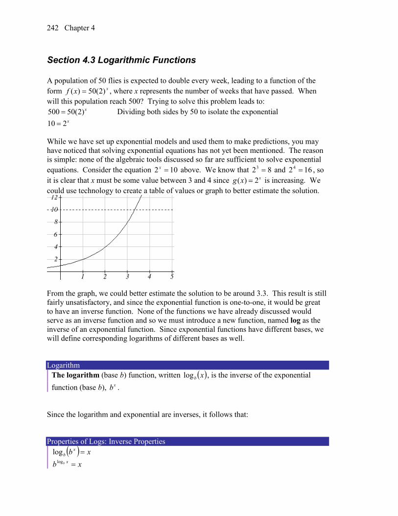
Section 4.3 Logarithmic Functions A population of 50 flies is expected to double every week, leading to a function of the form xxf )2(50)( = , where x represents the number of weeks that have passed. When will this population reach 500? Trying to solve this problem leads to: 500 50(2)x= Dividing both sides by 50 to isolate the exponential 10 2x= While we have set up exponential models and used them to make predictions, you may have noticed that solving exponential equations has not yet been mentioned. The reason is simple: none of the algebraic tools discussed so far are sufficient to solve exponential equations. Consider the equation 102 =x above. We know that 823 = and 1624 = , so it is clear that x must be some value between 3 and 4 since ( ) 2xg x = is increasing. We could use technology to create a table of values or graph to better estimate the solution.

From the graph, we could better estimate the solution to be around 3.3. This result is still fairly unsatisfactory, and since the exponential function is one-to-one, it would be great to have an inverse function. None of the functions we have already discussed would serve as an inverse function and so we must introduce a new function, named log as the inverse of an exponential function. Since exponential functions have different bases, we will define corresponding logarithms of different bases as well. Logarithm

The logarithm (base b) function, written ( )xblog , is the inverse of the exponential function (base b), xb .

Since the logarithm and exponential are inverses, it follows that: Properties of Logs: Inverse Properties

( ) xb xb =log

xb xb =log

Section 4.3 Logarithmic Functions 243

Recall also from the definition of an inverse function that if caf =)( , then acf =− )(1 . Applying this to the exponential and logarithmic functions: Logarithm Equivalent to an Exponential

The statement cba = is equivalent to the statement acb =)(log . Alternatively, we could show this by starting with the exponential function ac b= , then taking the log base b of both sides, giving log ( ) log a

b bc b= . Using the inverse property of logs we see that log ( )b c a= . Since log is a function, it is most correctly written as )(log cb , using parentheses to denote function evaluation, just as we would with f(c). However, when the input is a single variable or number, it is common to see the parentheses dropped and the expression written as cblog . Example 1

Write these exponential equations as logarithmic equations:

823 = 2552 = 10000

110 4 =−

823 = is equivalent to 3)8(log2 =

2552 = is equivalent to 2)25(log5 =

4 11010000

− = is equivalent to 101log 4

10000 = −

Example 2

Write these logarithmic equations as exponential equations:

( )216log6 = ( ) 29log3 =

( )216log6 = is equivalent to 66 2/1 =

( ) 29log3 = is equivalent to 932 = Try it Now

Write the exponential equation 1642 = as a logarithmic equation.

Chapter 4 244

By establishing the relationship between exponential and logarithmic functions, we can now solve basic logarithmic and exponential equations by rewriting. Example 3

Solve ( ) 2log4 =x for x. By rewriting this expression as an exponential, x=24 , so x = 16

Example 4

Solve 102 =x for x. By rewriting this expression as a logarithm, we get )10(log2=x

While this does define a solution, and an exact solution at that, you may find it somewhat unsatisfying since it is difficult to compare this expression to the decimal estimate we made earlier. Also, giving an exact expression for a solution is not always useful – often we really need a decimal approximation to the solution. Luckily, this is a task calculators and computers are quite adept at. Unluckily for us, most calculators and computers will only evaluate logarithms of two bases. Happily, this ends up not being a problem, as we’ll see briefly. Common and Natural Logarithms

The common log is the logarithm with base 10, and is typically written )log(x . The natural log is the logarithm with base e, and is typically written )ln(x .

Example 5

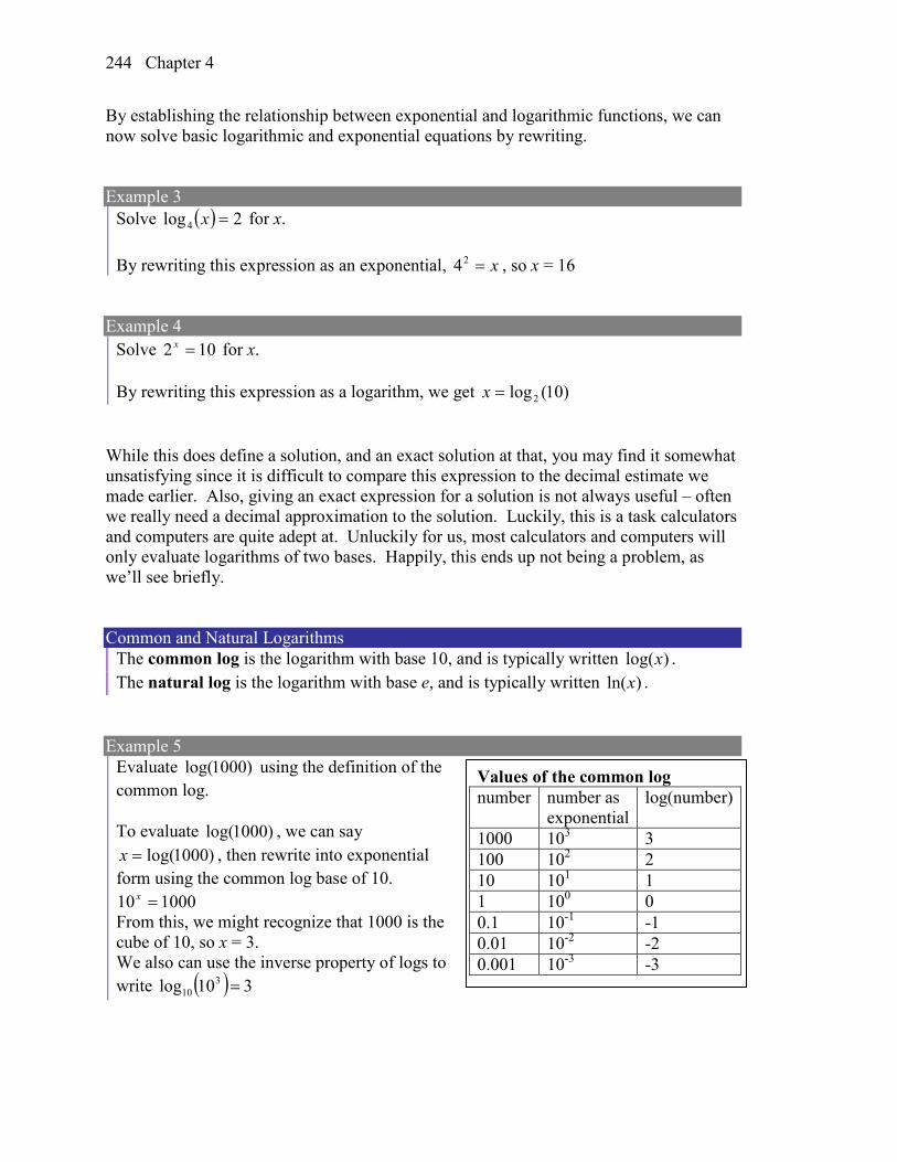
Evaluate )1000log( using the definition of the common log. To evaluate )1000log( , we can say

)1000log(=x , then rewrite into exponential form using the common log base of 10.

100010 =x From this, we might recognize that 1000 is the cube of 10, so x = 3. We also can use the inverse property of logs to write ( ) 310log 3

10 =

Values of the common log number number as

exponential log(number)

1000 103 3 100 102 2 10 101 1 1 100 0 0.1 10-1 -1 0.01 10-2 -2 0.001 10-3 -3


Try it Now 2. Evaluate )1000000log( .

Example 6

Evaluate ( )eln . We can rewrite ( )eln as ( )2/1ln e . Since ln is a log base e, we can use the inverse

property for logs: ( ) ( )21logln 2/12/1 == ee e .

Example 7

Evaluate log(500) using your calculator or computer. Using a computer, we can evaluate 69897.2)500log( ≈

To utilize the common or natural logarithm functions to evaluate expressions like

)10(log2 , we need to establish some additional properties. Properties of Logs: Exponent Property

( ) ( )ArA br

b loglog = To show why this is true, we offer a proof. Since the logarithmic and exponential functions are inverses, Ab Ab =log . So ( )rAr bbA log=

Utilizing the exponential rule that states ( )qp pqx x= ,

( ) ArrAr bb bbA loglog == So then ( ) ( )Ar

br

bbbA logloglog =

Again utilizing the inverse property on the right side yields the result ( ) ArA b

rb loglog =

Example 8

Rewrite ( )25log3 using the exponent property for logs. Since 25 = 52,

( ) ( ) 5log25log25log 32

33 ==

Chapter 4 246

Example 9 Rewrite )ln(4 x using the exponent property for logs. Using the property in reverse, ( )4ln)ln(4 xx =

Try it Now

3. Rewrite using the exponent property for logs:

2

1lnx

.

The exponent property allows us to find a method for changing the base of a logarithmic expression. Properties of Logs: Change of Base

( ))(log)(log

logbA

Ac

cb =

Proof: Let ( ) xAb =log . Rewriting as an exponential gives Ab x = . Taking the log base c of both sides of this equation gives

Ab cx

c loglog = Now utilizing the exponent property for logs on the left side,

Abx cc loglog = Dividing, we obtain

bA

xc

c

loglog

= or replacing our expression for x, bA

Ac

cb log

loglog =

With this change of base formula, we can finally find a good decimal approximation to our question from the beginning of the section. Example 10

Evaluate )10(log2 using the change of base formula. According to the change of base formula, we can rewrite the log base 2 as a logarithm of any other base. Since our calculators can evaluate the natural log, we might choose to use the natural logarithm, which is the log base e:

2ln10ln

2log10log

10log2 ==e

e

Using our calculators to evaluate this,


3219.369315.030259.2

2ln10ln

≈≈

This finally allows us to answer our original question – the population of flies we discussed at the beginning of the section will take 3.32 weeks to grow to 500.

Example 11

Evaluate )100(log5 using the change of base formula. We can rewrite this expression using any other base. If our calculators are able to evaluate the common logarithm, we could rewrite using the common log, base 10.

861.269897.0

25log

100log)100(log

10

105 =≈=

While we were able to solve the basic exponential equation 102 =x by rewriting in logarithmic form and then using the change of base formula to evaluate the logarithm, the proof of the change of base formula illuminates an alternative approach to solving exponential equations. Solving exponential equations:

1. Isolate the exponential expressions when possible 2. Take the logarithm of both sides 3. Utilize the exponent property for logarithms to pull the variable out of the exponent 4. Use algebra to solve for the variable.

Example 12

Solve 102 =x for x. Using this alternative approach, rather than rewrite this exponential into logarithmic form, we will take the logarithm of both sides of the equation. Since we often wish to evaluate the result to a decimal answer, we will usually utilize either the common log or natural log. For this example, we’ll use the natural log: ( ) )10ln(2ln =x Utilizing the exponent property for logs, ( ) )10ln(2ln =x Now dividing by ln(2),

( )ln(10) 2.861ln 2

x = ≈

Notice that this result matches the result we found using the change of base formula.

Chapter 4 248

Example 13 In the first section, we predicted the population (in billions) of India t years after 2008 by using the function ttf )0134.01(14.1)( += . If the population continues following this trend, when will the population reach 2 billion? We need to solve for the t so that f(t) = 2

t)0134.1(14.12 = Divide by 1.14 to isolate the exponential expression t0134.1

14.12

= Take the logarithm of both sides of the equation

( )t0134.1ln14.12ln =

Apply the exponent property on the right side

( )0134.1ln14.12ln t=

Divide both sides by ln(1.0134)

( ) 23.420134.1ln14.12ln

≈

=t years

If this growth rate continues, the model predicts the population of India will reach 2 billion about 42 years after 2008, or approximately in the year 2050.

Try it Now

4. Solve 10)93.0(5 =x . In addition to solving exponential equations, logarithmic expressions are common in many physical situations. Example 14

In chemistry, pH is a measure of the acidity or basicity of a liquid. The pH is related to the concentration of hydrogen ions, [H+], measured in moles per liter, by the equation

( )logpH H + = − .

If a liquid has concentration of 0.0001 moles per liber, determine the pH. Determine the hydrogen ion concentration of a liquid with pH of 7. To answer the first question, we evaluate the expression ( )0001.0log− . While we could use our calculators for this, we do not really need them here, since we can use the inverse property of logs:

( ) ( ) 4)4(10log0001.0log 4 =−−=−=− −


To answer the second question, we need to solve the equation ( )7 log H + = − . Begin

by isolating the logarithm on one side of the equation by multiplying both sides by -1:

( )7 log H + − =

Rewriting into exponential form yields the answer

710 0.0000001H + − = = moles per liter. Logarithms also provide us a mechanism for finding continuous growth models for exponential growth given two data points. Example 15

A population grows from 100 to 130 in 2 weeks. Find the continuous growth rate. Measuring t in weeks, we are looking for an equation rtaetP =)( so that P(0) = 100 and P(2) = 130. Using the first pair of values,

0100 rae ⋅= , so a = 100. Using the second pair of values,

2130 100 re ⋅= Divide by 100 2

100130 re= Take the natural log of both sides

( )2ln)3.1ln( re= Use the inverse property of logs

1312.02

)3.1ln(2)3.1ln(

≈=

=

r

r

This population is growing at a continuous rate of 13.12% per week. In general, we can relate the standard form of an exponential with the continuous growth form by noting (using k to represent the continuous growth rate to avoid the confusion of using r in two different ways in the same formula):

kxx aera =+ )1( kxx er =+ )1(

ker =+1 Using this, we see that it is always possible to convert from the continuous growth form of an exponential to the standard form and vice versa. Remember that the continuous growth rate k represents the nominal growth rate before accounting for the effects of continuous compounding, while r represents the actual percent increase in one time unit (one week, one year, etc.).

Chapter 4 250

Example 16 A company’s sales can be modeled by the function tetS 12.05000)( = , with t measured in years. Find the annual growth rate. Noting that ker =+1 , then 1275.0112.0 =−= er , so the annual growth rate is 12.75%. The sales function could also be written in the form ttS )1275.01(5000)( += .

Important Topics of this Section

The Logarithmic function as the inverse of the exponential function Writing logarithmic & exponential expressions Properties of logs Inverse properties Exponential properties Change of base Common log Natural log Solving exponential equations

Try it Now Answers

1. ( ) 4log24log216log 42

44 === 2. 6 3. )ln(2 x−

4. 5513.9)93.0ln(

)2ln(−≈


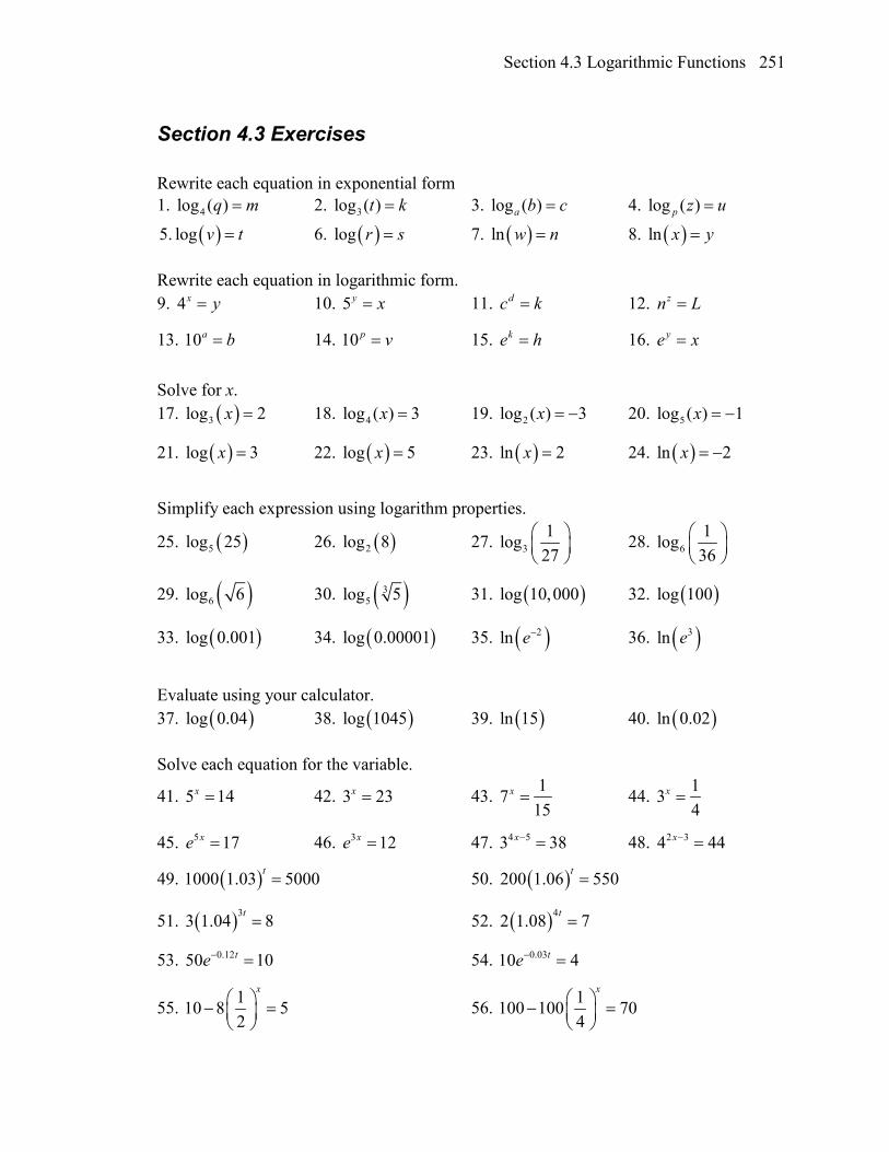
Section 4.3 Exercises Rewrite each equation in exponential form 1. 4log ( )q m= 2. 3log ( )t k= 3. log ( )a b c= 4. log ( )p z u=

( )5. log v t= 6. ( )log r s= 7. ( )ln w n= 8. ( )ln x y= Rewrite each equation in logarithmic form. 9. 4x y= 10. 5y x= 11. dc k= 12. zn L=

13. 10a b= 14. 10 p v= 15. ke h= 16. ye x=

Solve for x. 17. ( )3log 2x = 18. 4log ( ) 3x = 19. 2log ( ) 3x = − 20. 5log ( ) 1x = −

21. ( )log 3x = 22. ( )log 5x = 23. ( )ln 2x = 24. ( )ln 2x = −

Simplify each expression using logarithm properties.

25. ( )5log 25 26. ( )2log 8 27. 31log27

28. 61log36

29. ( )6log 6 30. ( )35log 5 31. ( )log 10,000 32. ( )log 100

33. ( )log 0.001 34. ( )log 0.00001 35. ( )2ln e− 36. ( )3ln e

Evaluate using your calculator. 37. ( )log 0.04 38. ( )log 1045 39. ( )ln 15 40. ( )ln 0.02 Solve each equation for the variable.

41. 5 14x = 42. 3 23x = 43. 1715

x = 44. 134

x =

45. 5 17xe = 46. 3 12xe = 47. 4 53 38x− = 48. 2 34 44x− =

49. ( )1000 1.03 5000t = 50. ( )200 1.06 550t =

51. ( )33 1.04 8t = 52. ( )42 1.08 7t =

53. 0.1250 10te− = 54. 0.0310 4te− =

55. 110 8 52

x − =

56. 1100 100 704

x − =

Chapter 4 252

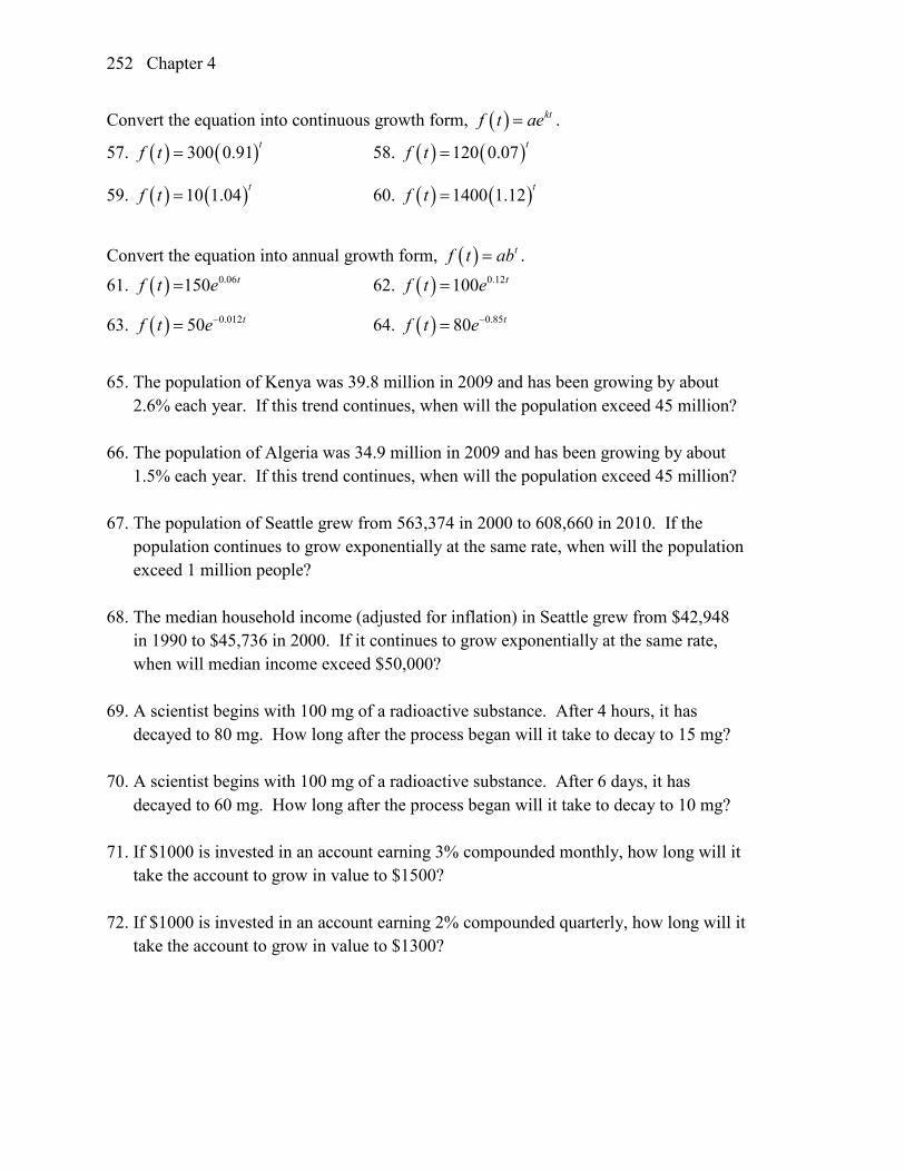
Convert the equation into continuous growth form, ( ) ktf t ae= .

57. ( ) ( )300 0.91 tf t = 58. ( ) ( )120 0.07 tf t =

59. ( ) ( )10 1.04 tf t = 60. ( ) ( )1400 1.12 tf t =

Convert the equation into annual growth form, ( ) tf t ab= .

61. ( ) 0.061 50 tf t e= 62. ( ) 0.12100 tf t e=

63. ( ) 0.01250 tf t e−= 64. ( ) 0.8580 tf t e−=

65. The population of Kenya was 39.8 million in 2009 and has been growing by about

2.6% each year. If this trend continues, when will the population exceed 45 million?

66. The population of Algeria was 34.9 million in 2009 and has been growing by about 1.5% each year. If this trend continues, when will the population exceed 45 million?

67. The population of Seattle grew from 563,374 in 2000 to 608,660 in 2010. If the population continues to grow exponentially at the same rate, when will the population exceed 1 million people?

68. The median household income (adjusted for inflation) in Seattle grew from $42,948 in 1990 to $45,736 in 2000. If it continues to grow exponentially at the same rate, when will median income exceed $50,000?

69. A scientist begins with 100 mg of a radioactive substance. After 4 hours, it has decayed to 80 mg. How long after the process began will it take to decay to 15 mg?

70. A scientist begins with 100 mg of a radioactive substance. After 6 days, it has decayed to 60 mg. How long after the process began will it take to decay to 10 mg?

71. If $1000 is invested in an account earning 3% compounded monthly, how long will it take the account to grow in value to $1500?

72. If $1000 is invested in an account earning 2% compounded quarterly, how long will it take the account to grow in value to $1300?

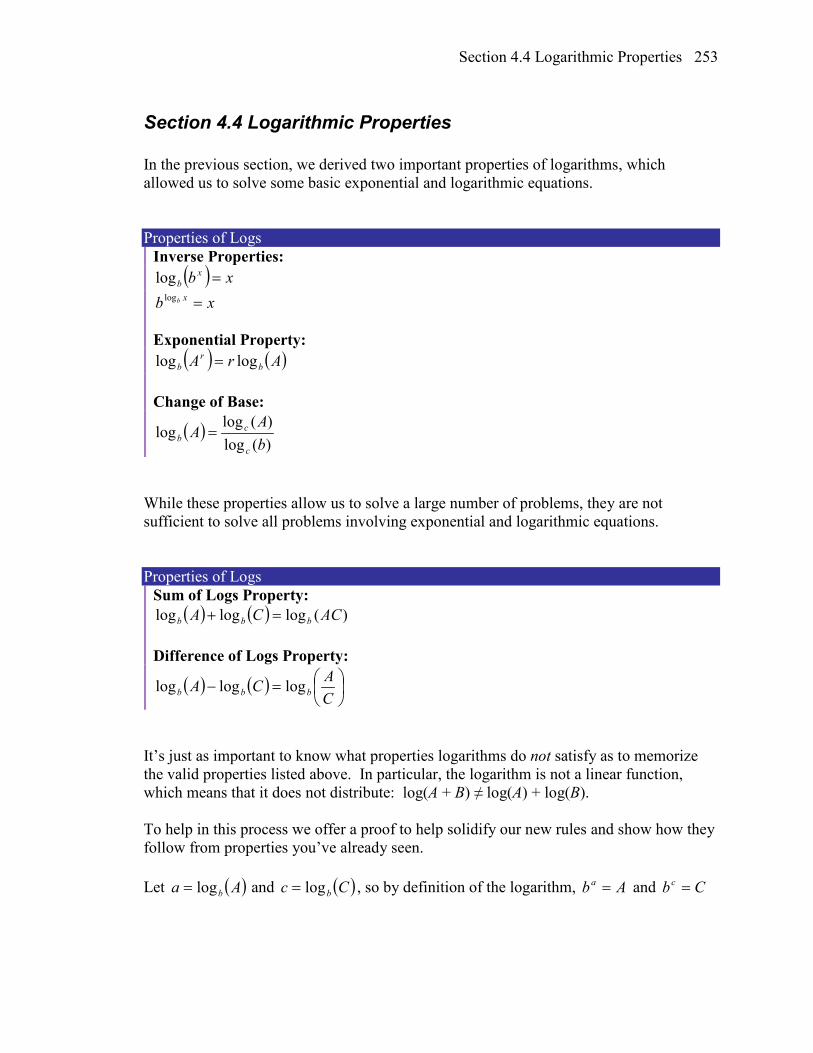
Section 4.4 Logarithmic Properties 253

Section 4.4 Logarithmic Properties In the previous section, we derived two important properties of logarithms, which allowed us to solve some basic exponential and logarithmic equations. Properties of Logs

Inverse Properties: ( ) xb x

b =log xb xb =log

Exponential Property:

( ) ( )ArA br

b loglog = Change of Base:

( ))(log)(log

logbA

Ac

cb =

While these properties allow us to solve a large number of problems, they are not sufficient to solve all problems involving exponential and logarithmic equations. Properties of Logs

Sum of Logs Property: ( ) ( ) )(logloglog ACCA bbb =+

Difference of Logs Property:

( ) ( )

=−

CACA bbb logloglog

It’s just as important to know what properties logarithms do not satisfy as to memorize the valid properties listed above. In particular, the logarithm is not a linear function, which means that it does not distribute: log(A + B) ≠ log(A) + log(B). To help in this process we offer a proof to help solidify our new rules and show how they follow from properties you’ve already seen. Let ( )Aa blog= and ( )Cc blog= , so by definition of the logarithm, Aba = and Cbc =

Chapter 4 254

Using these expressions, cabbAC = Using exponent rules on the right, cabAC += Taking the log of both sides, and utilizing the inverse property of logs,

( ) ( ) cabAC cabb +== +loglog

Replacing a and c with their definition establishes the result ( ) CAAC bbb logloglog +=

The proof for the difference property is very similar. With these properties, we can rewrite expressions involving multiple logs as a single log, or break an expression involving a single log into expressions involving multiple logs. Example 1

Write ( ) ( ) ( )2log8log5log 333 −+ as a single logarithm. Using the sum of logs property on the first two terms,

( ) ( ) ( ) ( )40log85log8log5log 3333 =⋅=+ This reduces our original expression to ( ) ( )2log40log 33 − Then using the difference of logs property,

( ) ( ) ( )20log240log2log40log 3333 =

=−

Example 2

Evaluate ( ) ( )4log5log2 + without a calculator by first rewriting as a single logarithm. On the first term, we can use the exponent property of logs to write

( ) ( ) ( )25log5log5log2 2 == With the expression reduced to a sum of two logs, ( ) ( )4log25log + , we can utilize the sum of logs property

( ) ( ) )100log()254log(4log25log =⋅=+ Since 100 = 102, we can evaluate this log without a calculator:

( ) 210log)100log( 2 == Try it Now

1. Without a calculator evaluate by first rewriting as a single logarithm: ( ) ( )4log8log 22 +


Example 3

Rewrite

7

ln4 yx as a sum or difference of logs

First, noticing we have a quotient of two expressions, we can utilize the difference property of logs to write

( ) )7ln(ln7

ln 44

−=

yxyx

Then seeing the product in the first term, we use the sum property ( ) ( ) )7ln()ln(ln)7ln(ln 44 −+=− yxyx

Finally, we could use the exponent property on the first term ( ) )7ln()ln()ln(4)7ln()ln(ln 4 −+=−+ yxyx

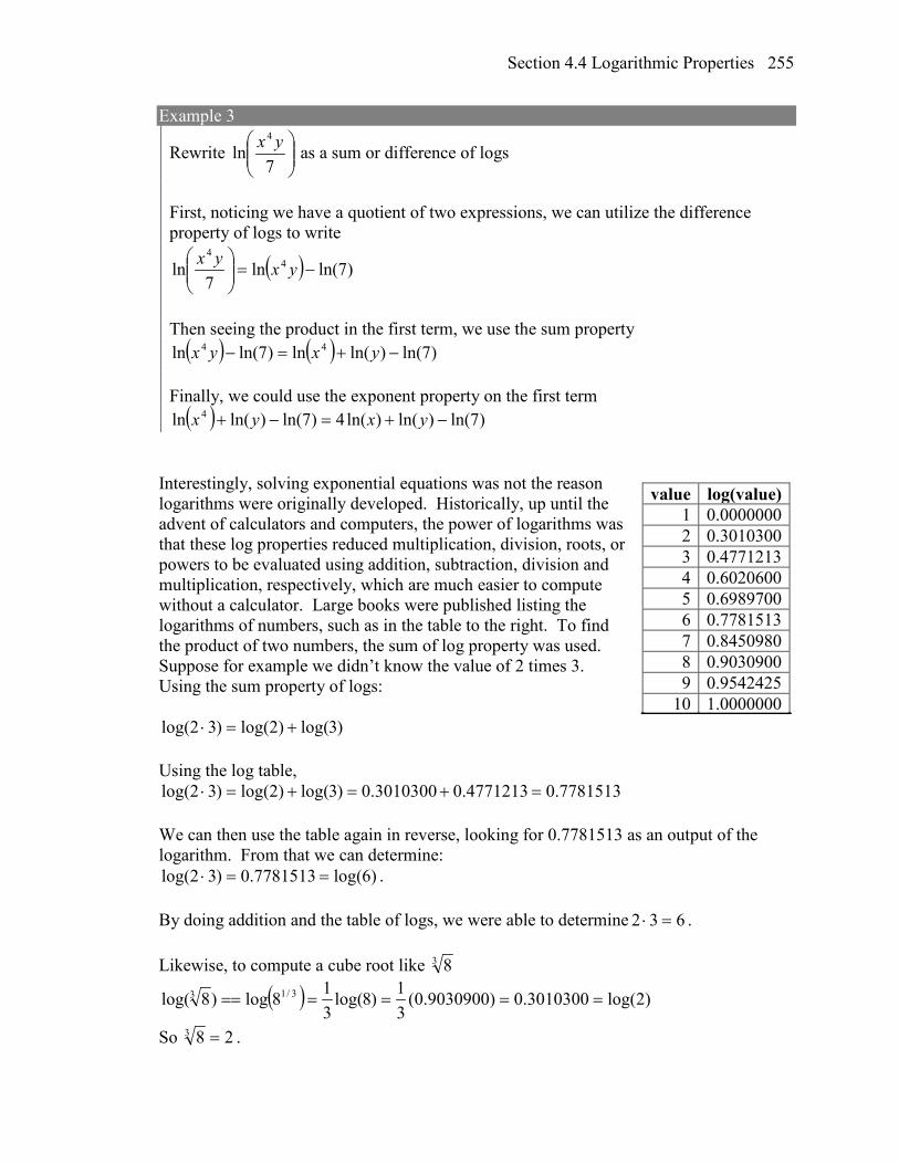
Interestingly, solving exponential equations was not the reason logarithms were originally developed. Historically, up until the advent of calculators and computers, the power of logarithms was that these log properties reduced multiplication, division, roots, or powers to be evaluated using addition, subtraction, division and multiplication, respectively, which are much easier to compute without a calculator. Large books were published listing the logarithms of numbers, such as in the table to the right. To find the product of two numbers, the sum of log property was used. Suppose for example we didn’t know the value of 2 times 3. Using the sum property of logs:

)3log()2log()32log( +=⋅ Using the log table,

7781513.04771213.03010300.0)3log()2log()32log( =+=+=⋅ We can then use the table again in reverse, looking for 0.7781513 as an output of the logarithm. From that we can determine:

)6log(7781513.0)32log( ==⋅ . By doing addition and the table of logs, we were able to determine 632 =⋅ . Likewise, to compute a cube root like 3 8

( ) )2log(3010300.0)9030900.0(31)8log(

318log)8log( 3/13 ======

So 283 = .

value log(value) 1 0.0000000 2 0.3010300 3 0.4771213 4 0.6020600 5 0.6989700 6 0.7781513 7 0.8450980 8 0.9030900 9 0.9542425

10 1.0000000

Chapter 4 256

Although these calculations are simple and insignificant they illustrate the same idea that was used for hundreds of years as an efficient way to calculate the product, quotient, roots, and powers of large and complicated numbers, either using tables of logarithms or mechanical tools called slide rules. These properties still have other practical applications for interpreting changes in exponential and logarithmic relationships. Example 4

Recall that in chemistry, ( )logpH H + = − . If the concentration of hydrogen ions in a

liquid is doubled, what is the affect on pH? Suppose C is the original concentration of hydrogen ions, and P is the original pH of the liquid, so ( )CP log−= . If the concentration is doubled, the new concentration is 2C. Then the pH of the new liquid is

( )CpH 2log−= Using the sum property of logs,

( ) ( ) )log()2log()log()2log(2log CCCpH −−=+−=−= Since ( )CP log−= , the new pH is

301.0)2log( −=−= PPpH When the concentration of hydrogen ions is doubled, the pH decreases by 0.301.

Log properties in solving equations The logarithm properties often arise when solving problems involving logarithms. Example 5

Solve 2)log()2550log( =−+ xx . In order to rewrite in exponential form, we need a single logarithmic expression on the left side of the equation. Using the difference property of logs, we can rewrite the left side:

22550log =

+

xx

Rewriting in exponential form reduces this to an algebraic equation:

100102550 2 ==+x

x


Solving,

21

50255025

1002550

==

==+

x

xxx

Checking this answer in the original equation, we can verify there are no domain issues, and this answer is correct.

Try it Now

2. Solve )2log(1)4log( 2 ++=− xx . More complex exponential equations can often be solved in more than one way. In the following example, we will solve the same problem in two ways – one using logarithm properties, and the other using exponential properties. Example 6a

In 2008, the population of Kenya was approximately 38.8 million, and was growing by 2.64% each year, while the population of Sudan was approximately 41.3 million and growing by 2.24% each year2. If these trends continue, when will the population of Kenya match that of Sudan? We start by writing an equation for each population in terms of t, the number of years after 2008.

( ) 38.8(1 0.0264)( ) 41.3(1 0.0224)

t

t

Kenya tSudan t

= +

= +

To find when the populations will be equal, we can set the equations equal 38.8(1.0264) 41.3(1.0224)t t= For our first approach, we take the log of both sides of the equation

( ) ( )log 38.8(1.0264) log 41.3(1.0224)t t= Utilizing the sum property of logs, we can rewrite each side,

( ) ( )log(38.8) log 1.0264 log(41.3) log 1.0224t t+ = + Then utilizing the exponent property, we can pull the variables out of the exponent

2 World Bank, World Development Indicators, as reported on http://www.google.com/publicdata, retrieved August 24, 2010

http://www.google.com/publicdata

Chapter 4 258

( ) ( )log(38.8) log 1.0264 log(41.3) log 1.0224t t+ = + Moving all the terms involving t to one side of the equation and the rest of the terms to the other side,

( ) ( )log 1.0264 log 1.0224 log(41.3) log(38.8)t t− = − Factoring out the t on the left,

( ) ( )( )log 1.0264 log 1.0224 log(41.3) log(38.8)t − = − Dividing to solve for t

( ) ( )log(41.3) log(38.8) 15.991

log 1.0264 log 1.0224t −= ≈

−years until the populations will be equal.

Example 6b

Solve the problem above by rewriting before taking the log. Starting at the equation 38.8(1.0264) 41.3(1.0224)t t= Divide to move the exponential terms to one side of the equation and the constants to the other side 1.0264 41.31.0224 38.8

t

t =

Using exponent rules to group on the left,

1.0264 41.31.0224 38.8

t =

Taking the log of both sides

1.0264 41.3log log1.0224 38.8

t =

Utilizing the exponent property on the left,

1.0264 41.3log log1.0224 38.8

t =

Dividing gives

41.3log38.8 15.991

1.0264log1.0224

t

= ≈

years


While the answer does not immediately appear identical to that produced using the previous method, note that by using the difference property of logs, the answer could be rewritten:

41.3loglog(41.3) log(38.8)38.8

1.0264 log(1.0264) log(1.0224)log1.0224

t

− = =

−

While both methods work equally well, it often requires fewer steps to utilize algebra before taking logs, rather than relying solely on log properties. Try it Now

3. Tank A contains 10 liters of water, and 35% of the water evaporates each week. Tank B contains 30 liters of water, and 50% of the water evaporates each week. In how many weeks will the tanks contain the same amount of water?

Important Topics of this Section

Inverse Exponential Change of base Sum of logs property Difference of logs property Solving equations using log rules

Try it Now Answers

1. 5 2. 12 3. 4.1874 weeks

Chapter 4 260

Section 4.4 Exercises Simplify to a single logarithm, using logarithm properties. 1. ( ) ( )3 3log 28 log 7− 2. ( ) ( )3 3log 32 log 4−

3. 31log7

−

4. 41log5

−

5. ( )3 31log log 50

10 +

6. ( )4 4log 3 log (7)+

7. ( )71 log 83

8. ( )51 log 362

9. ( ) ( )4 5log 2 log 3x x+ 10. ( ) ( )2 3ln 4 ln 3x x+

11. ( ) ( )9 2ln 6 ln 3x x− 12. ( ) ( )4log 12 log 4x x−

13. ( ) ( )2log 3log 1x x+ + 14. ( ) ( )23log 2logx x+

15. ( ) ( ) ( )1log log 3log2

x y z− + 16. ( ) ( ) ( )12log log log3

x y z+ −

Use logarithm properties to expand each expression.

17. 15 13

19log x yz

18. 2 3

5log a bc

19. 2

4 5ln ab c

−

−

20. 2 3

5ln a bc

−

−

21. ( )3 4log x y− 22. ( )3 2log x y−

23. ln1

yyy

−

24. 2

ln1

xx

−

25. ( )2 3 2 53log x y x y 26. ( )3 4 3 97log x y x y


Solve each equation for the variable. 27. 4 7 9 64 3x x− −= 28. 2 5 3 72 7x x− −=

29. ( ) ( )17 1.14 19 1.16x x= 30. ( ) ( )20 1.07 8 1.13x x=

31. 0.12 0.085 10t te e= 32. 0.09 0.143 t te e=

33. ( )2log 7 6 3x + = 34. 3log (2 4) 2x + =

35. ( )2ln 3x 3 1+ = 36. ( )4ln 5 5 2x + =

37. ( )3log 2x = 38. ( )5log 3x =

39. ( ) ( )log log 3 3x x+ + = 40. ( ) ( )log 4 log 9x x+ + =

41. ( ) ( )log 4 log 3 1x x+ − + = 42. ( ) ( )log 5 log 2 2x x+ − + =

43. ( )26 6log log ( 1) 1x x− + = 44. 2

3 3log ( ) log ( 2) 5x x− + =

45. ( ) ( ) ( )log 12 log log 12x x+ = + 46. ( ) ( ) ( )log 15 log log 15x x+ = +

47. ( ) ( ) ( )ln ln 3 ln 7x x x+ − = 48. ( ) ( ) ( )ln ln 6 ln 6x x x+ − =

Documents

Chapter 4: Exponential and Logarithmic Functions · 2015-02-02 · Chapter 4: Exponential and Logarithmic Functions Section 4.1 Exponential Functions ... 216 Chapter 4 Notice that