Embed Size (px)
Citation preview
74
Chapter 4: Generating Functions
This chapter looks at Probability Generating Functions (PGFs) for discrete
random variables. PGFs are useful tools for dealing with sums and limits of
random variables. For some stochastic processes, they also have a special rolein telling us whether a process will ever reach a particular state.
By the end of this chapter, you should be able to:
• find the sum of Geometric, Binomial, and Exponential series;
• know the definition of the PGF, and use it to calculate the mean, variance,
and probabilities;
• calculate the PGF for Geometric, Binomial, and Poisson distributions;
• calculate the PGF for a randomly stopped sum;
• calculate the PGF for first reaching times in the random walk;
• use the PGF to determine whether a process will ever reach a given state.
4.1 Common sums
1. Geometric Series
1 + r + r2 + r3 + . . . =
∞∑
x=0
rx =1
1− r, when|r| < 1.
This formula proves that∑∞
x=0 P(X = x) = 1 when X ∼ Geometric(p):
P(X = x) = p(1− p)x ⇒∞∑
x=0
P(X = x) =∞∑
x=0
p(1− p)x
= p∞∑
x=0
(1− p)x
=p
1− (1− p)(because|1− p| < 1)
= 1.
75
2. Binomial Theorem For anyp, q ∈ R, and integern,
(p+ q)n =
n∑
x=0
(
n
x
)
pxqn−x.
Note that(
n
x
)
=n!
(n− x)! x!(nCr button on calculator.)
The Binomial Theorem proves that∑n
x=0 P(X = x) = 1 whenX ∼ Binomial(n, p):
P(X = x) =
(
n
x
)
px(1− p)n−x for x = 0, 1, . . . , n, so
n∑
x=0
P(X = x) =
n∑
x=0
(
n
x
)
px(1− p)n−x
=(
p+ (1− p))n
= 1n
= 1.
3. Exponential Power Series
For anyλ ∈ R,∞∑
x=0
λx
x!= eλ.
This proves that∑∞
x=0 P(X = x) = 1 when X ∼ Poisson(λ):
P(X = x) =λx
x!e−λ for x = 0, 1, 2, . . ., so
∞∑
x=0
P(X = x) =∞∑
x=0
λx
x!e−λ = e−λ
∞∑
x=0
λx
x!
= e−λ eλ
= 1.
Note: Another useful identity is: eλ = limn→∞
(
1 +λ
n
)n
for λ ∈ R.
76
4.2 Probability Generating Functions
The probability generating function (PGF) is a useful tool for dealing
with discrete random variables taking values 0, 1, 2, . . .. Its particular strengthis that it gives us an easy way of characterizing the distribution of X +Y when
X and Y are independent. In general it is difficult to find the distribution ofa sum using the traditional probability function. The PGF transforms a sum
into a product and enables it to be handled much more easily.
Sums of random variables are particularly important in the study of stochastic
processes, because many stochastic processes are formed from the sum of asequence of repeating steps: for example, the Gambler’s Ruin from Section 2.7.
The name probability generating function also gives us another clue to the role
of the PGF. The PGF can be used to generate all the probabilities of thedistribution. This is generally tedious and is not often an efficient way of
calculating probabilities. However, the fact that it can be done demonstratesthat the PGF tells us everything there is to know about the distribution.
Definition: Let X be a discrete random variable taking values in the non-negative
integers {0, 1, 2, . . .}. The probability generating function (PGF) of X is
GX(s) = E(sX), for all s ∈ R for which the sum converges.
Calculating the probability generating function
GX(s) = E(
sX)
=
∞∑
x=0
sxP(X = x).
Properties of the PGF:
1. GX(0) = P(X = 0):
GX(0) = 00 × P(X = 0) + 01 × P(X = 1) + 02 × P(X = 2) + . . .
∴ GX(0) = P(X = 0).
77
2. GX(1) = 1 : GX(1) =∞∑
x=0
1xP(X = x) =∞∑
x=0
P(X = x) = 1.
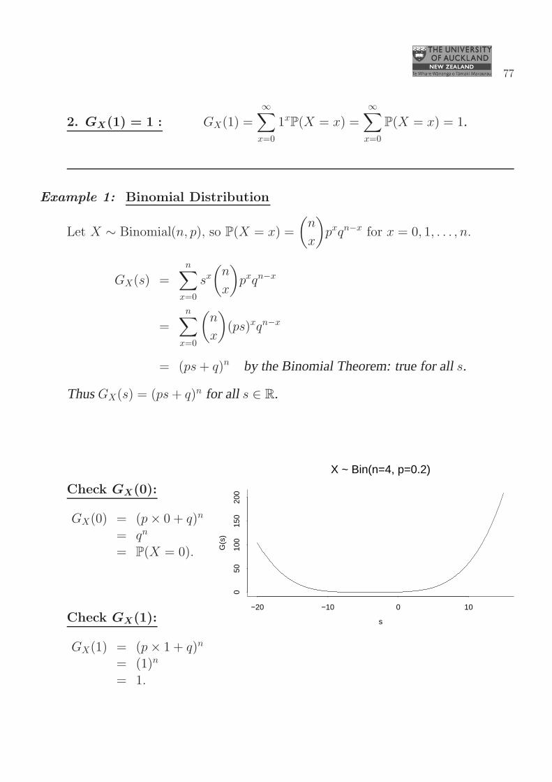
Example 1: Binomial Distribution
Let X ∼ Binomial(n, p), so P(X = x) =
(
n
x
)
pxqn−x for x = 0, 1, . . . , n.
GX(s) =n∑
x=0
sx(
n
x
)
pxqn−x
=
n∑
x=0
(
n
x
)
(ps)xqn−x
= (ps+ q)n by the Binomial Theorem: true for alls.
ThusGX(s) = (ps+ q)n for all s ∈ R.
s
G(s
)
−20 −10 0 10
050
100
150
200
X ~ Bin(n=4, p=0.2)
Check GX(0):
GX(0) = (p× 0 + q)n
= qn
= P(X = 0).
Check GX(1):
GX(1) = (p× 1 + q)n
= (1)n
= 1.
78
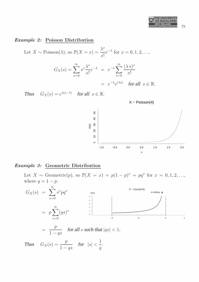
Example 2: Poisson Distribution
Let X ∼ Poisson(λ), so P(X = x) =λx
x!e−λ for x = 0, 1, 2, . . ..
GX(s) =∞∑
x=0
sxλx
x!e−λ = e−λ
∞∑
x=0
(λ s)x
x!
= e−λe(λs) for all s ∈ R.
Thus GX(s) = eλ(s−1) for all s ∈ R.
s
G(s
)
−1.0 −0.5 0.0 0.5 1.0 1.5 2.0
010
2030
4050
X ~ Poisson(4)
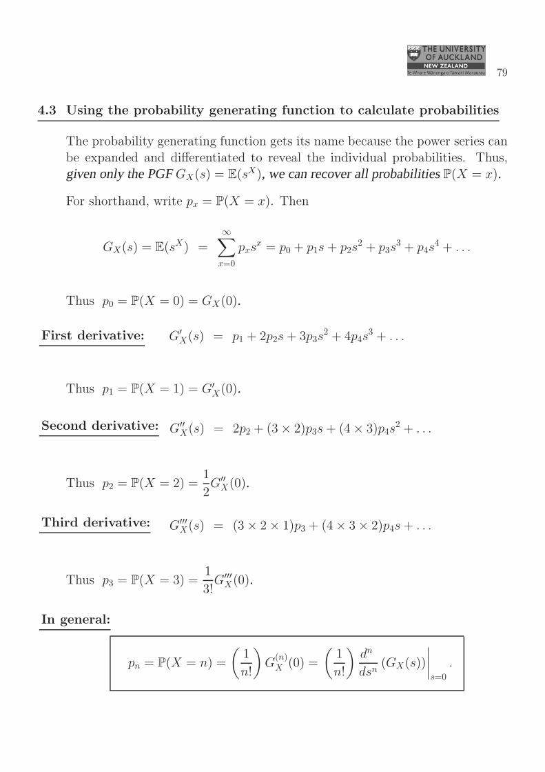
Example 3: Geometric Distribution
Let X ∼ Geometric(p), so P(X = x) = p(1 − p)x = pqx for x = 0, 1, 2, . . .,where q = 1− p.
−5 0 5
01
23
45
G(s)
s
to infinityX ~ Geom(0.8)
GX(s) =
∞∑
x=0
sxpqx
= p∞∑
x=0
(qs)x
=p
1− qsfor all s such that|qs| < 1.
Thus GX(s) =p
1− qsfor |s| < 1
q.
79
4.3 Using the probability generating function to calculate probabilities
The probability generating function gets its name because the power series canbe expanded and differentiated to reveal the individual probabilities. Thus,
given only the PGFGX(s) = E(sX), we can recover all probabilitiesP(X = x).
For shorthand, write px = P(X = x). Then
GX(s) = E(sX) =∞∑
x=0
pxsx = p0 + p1s+ p2s
2 + p3s3 + p4s
4 + . . .
Thus p0 = P(X = 0) = GX(0).
First derivative: G′X(s) = p1 + 2p2s+ 3p3s
2 + 4p4s3 + . . .
Thus p1 = P(X = 1) = G′X(0).
Second derivative: G′′X(s) = 2p2 + (3× 2)p3s+ (4× 3)p4s
2 + . . .
Thus p2 = P(X = 2) =1
2G′′
X(0).
Third derivative: G′′′X(s) = (3× 2× 1)p3 + (4× 3× 2)p4s+ . . .
Thus p3 = P(X = 3) =1
3!G′′′
X(0).
In general:
pn = P(X = n) =
(
1
n!
)
G(n)X (0) =
(
1
n!
)
dn
dsn(GX(s))
∣
∣
∣
∣
s=0
.
80
Example: Let X be a discrete random variable with PGF GX(s) =s
5(2 + 3s2).
Find the distribution of X.
GX(s) =2
5s+
3
5s3 : GX(0) = P(X = 0) = 0.
G′X(s) =
2
5+
9
5s2 : G′
X(0) = P(X = 1) =2
5.
G′′X(s) =
18
5s :
1
2G′′
X(0) = P(X = 2) = 0.
G′′′X(s) =
18
5:
1
3!G′′′
X(0) = P(X = 3) =3
5.
G(r)X (s) = 0 ∀r ≥ 4 :
1
r!G
(r)X (s) = P(X = r) = 0 ∀r ≥ 4.
Thus
X =
{
1 with probability2/5,3 with probability3/5.
Uniqueness of the PGF
The formula pn = P(X = n) =
(
1
n!
)
G(n)X (0) shows that the whole sequence of
probabilities p0, p1, p2, . . . is determined by the values of the PGF and its deriv-atives at s = 0. It follows that the PGF specifies a unique set of probabilities.
Fact: If two power series agree on any interval containing 0, however small, thenall terms of the two series are equal.
Formally: letA(s) andB(s) be PGFs withA(s) =∑∞
n=0 ansn, B(s) =
∑∞n=0 bns
n.
If there exists some R′ > 0 such that A(s) = B(s) for all −R′ < s < R′, thenan = bn for all n.
Practical use: If we can show that two random variables have the same PGF insome interval containing 0, then we have shown that the two random variableshave the same distribution.
Another way of expressing this is to say that the PGF ofX tells us everythingthere is to know about the distribution ofX.
81
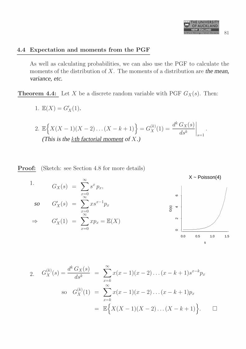
4.4 Expectation and moments from the PGF
As well as calculating probabilities, we can also use the PGF to calculate themoments of the distribution of X. The moments of a distribution are the mean,variance, etc.
Theorem 4.4: Let X be a discrete random variable with PGF GX(s). Then:
1. E(X) = G′X(1).
2. E{
X(X − 1)(X − 2) . . . (X − k + 1)}
= G(k)X (1) =
dk GX(s)
dsk
∣
∣
∣
∣
s=1
.
(This is thekth factorial momentof X.)
Proof: (Sketch: see Section 4.8 for more details)
1.GX(s) =
∞∑
x=0
sx px,
so G′X(s) =
∞∑
x=0
xsx−1px
⇒ G′X(1) =
∞∑
x=0
xpx = E(X)
s
G(s
)
0.0 0.5 1.0 1.5
02
46
X ~ Poisson(4)
2. G(k)X (s) =
dk GX(s)
dsk=
∞∑
x=k
x(x− 1)(x− 2) . . . (x− k + 1)sx−kpx
so G(k)X (1) =
∞∑
x=k
x(x− 1)(x− 2) . . . (x− k + 1)px
= E
{
X(X − 1)(X − 2) . . . (X − k + 1)}
. �
82
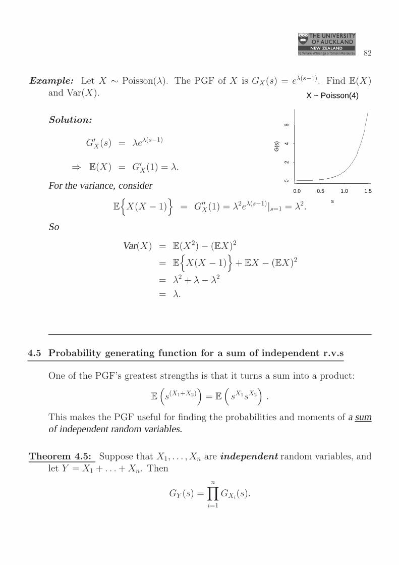
Example: Let X ∼ Poisson(λ). The PGF of X is GX(s) = eλ(s−1). Find E(X)and Var(X).
Solution:
s
G(s
)
0.0 0.5 1.0 1.5
02
46
X ~ Poisson(4)
G′X(s) = λeλ(s−1)
⇒ E(X) = G′X(1) = λ.
For the variance, consider
E
{
X(X − 1)}
= G′′X(1) = λ2eλ(s−1)|s=1 = λ2.
So
Var(X) = E(X2)− (EX)2
= E
{
X(X − 1)}
+ EX − (EX)2
= λ2 + λ− λ2
= λ.
4.5 Probability generating function for a sum of independent r.v.s
One of the PGF’s greatest strengths is that it turns a sum into a product:
E
(
s(X1+X2))
= E
(
sX1sX2
)
.
This makes the PGF useful for finding the probabilities and moments of a sumof independent random variables.
Theorem 4.5: Suppose that X1, . . . , Xn are independent random variables, andlet Y = X1 + . . .+Xn. Then
GY (s) =
n∏
i=1
GXi(s).
83
Proof: GY (s) = E(s(X1+...+Xn))
= E(sX1sX2 . . . sXn)
= E(sX1)E(sX2) . . .E(sXn)
(becauseX1, . . . , Xn are independent)
=
n∏
i=1
GXi(s). as required. �
Example: Suppose that X and Y are independent with X ∼ Poisson(λ) andY ∼ Poisson(µ). Find the distribution of X + Y .
Solution: GX+Y (s) = GX(s) ·GY (s)
= eλ(s−1)eµ(s−1)
= e(λ+µ)(s−1).
But this is the PGF of the Poisson(λ + µ) distribution. So, by the uniqueness ofPGFs,X + Y ∼ Poisson(λ+ µ).
4.6 Randomly stopped sum
Remember the randomly stopped sum model from
Section 3.4. A random number N of events occur,and each event i has associated with it a cost or
reward Xi. The question is to find the distributionof the total cost or reward: TN = X1 +X2 + . . .+XN .
TN is called a randomly stopped sum because it has a random number of terms.
Example: Cash machine model. N customers arrive during the day. Customer iwithdraws amount Xi. The total amount withdrawn during the day is TN =
X1 + . . .+XN .
84
In Chapter 3, we used the Laws of Total Expectation and Variance to showthat E(TN) = µE(N) and Var(TN) = σ2
E(N) + µ2Var(N), where µ = E(Xi)
and σ2 = Var(Xi).
In this chapter we will now use probability generating functions to investigatethe whole distribution ofTN .
Theorem 4.6: Let X1, X2, . . . be a sequence of independent and identically dis-tributed random variables with common PGF GX . LetN be a random variable,
independent of the Xi’s, with PGF GN , and let TN = X1+ . . .+XN =∑N
i=1Xi.Then the PGF of TN is:
GTN(s) = GN
(
GX(s))
.
Proof:
GTN(s) = E(sTN) = E
(
sX1+...+XN)
= EN
{
E
(
sX1+...+XN
∣
∣
∣N)}
(conditional expectation)
= EN
{
E(
sX1 . . . sXN |N)
}
= EN
{
E(
sX1 . . . sXN)
}
(Xi’s are indept ofN)
= EN
{
E(
sX1
)
. . .E(
sXN)
}
(Xi’s are indept of each other)
= EN
{
(GX(s))N}
= GN
(
GX(s))
(by definition ofGN ). �
85
Example: Let X1, X2, . . . and N be as above. Find the mean of TN .
E(TN) = G′TN(1) =
d
dsGN(GX(s))
∣
∣
∣
s=1
= G′N (GX(s)) ·G′
X(s)∣
∣
∣
s=1
= G′N (1) ·G′
X(1) Note:GX(1) = 1 for any r.v.X
= E(N) · E(X1), — same answer as in Chapter 3.
Example: Heron goes fishing
My aunt was asked by her neighbours to feed the prize
goldfish in their garden pond while they were on holiday.Although my aunt dutifully went and fed them every day,she never saw a single fish for the whole three weeks. It
turned out that all the fish had been eaten by a heronwhen she wasn’t looking!
Let N be the number of times the heron visits the pond
during the neighbours’ absence. Suppose that N ∼ Geometric(1− θ),so P(N = n) = (1 − θ)θn, for n = 0, 1, 2, . . .. When the heron visits the pond
it has probability p of catching a prize goldfish, independently of what happenson any other visit. (This assumes that there are infinitely many goldfish to becaught!) Find the distribution of
T = total number of goldfish caught.
Solution:
Let Xi =
{
1 if heron catches a fish on visiti,0 otherwise.
ThenT = X1 +X2 + . . .+XN (randomly stopped sum), so
GT (s) = GN(GX(s)).
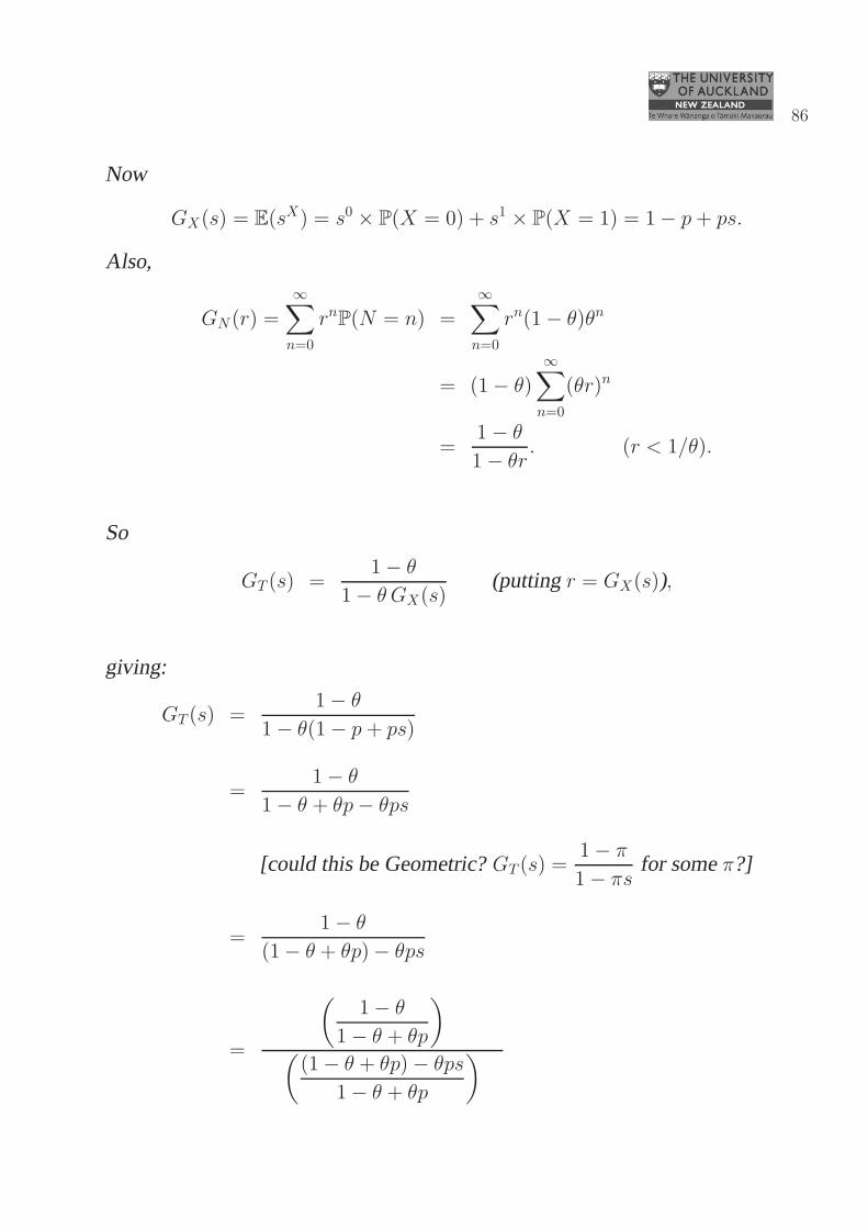
86
Now
GX(s) = E(sX) = s0 × P(X = 0) + s1 × P(X = 1) = 1− p+ ps.
Also,
GN (r) =∞∑
n=0
rnP(N = n) =∞∑
n=0
rn(1− θ)θn
= (1− θ)
∞∑
n=0
(θr)n
=1− θ
1− θr. (r < 1/θ).
So
GT (s) =1− θ
1− θ GX(s)(puttingr = GX(s)),
giving:
GT (s) =1− θ
1− θ(1− p + ps)
=1− θ
1− θ + θp− θps
[could this be Geometric?GT (s) =1− π
1− πsfor someπ?]
=1− θ
(1− θ + θp)− θps
=
(
1− θ
1− θ + θp
)
(
(1− θ + θp)− θps
1− θ + θp
)
87
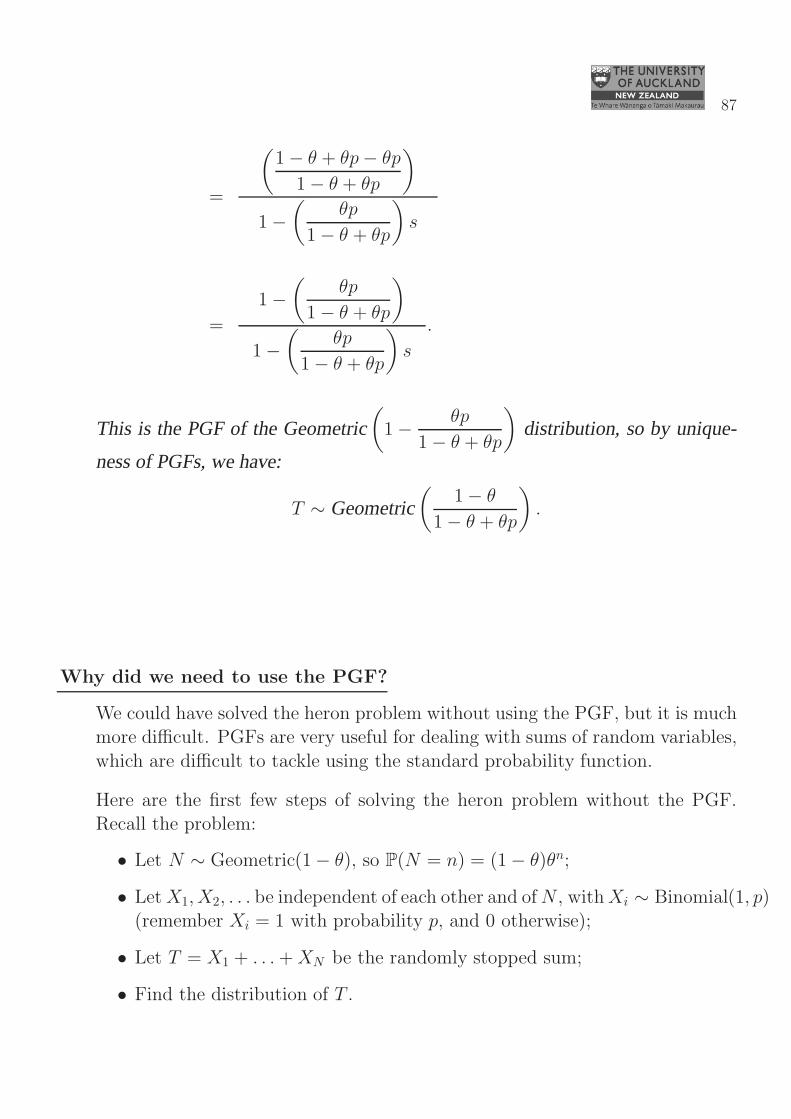
=
(
1− θ + θp− θp
1− θ + θp
)
1−(
θp
1− θ + θp
)
s
=
1−(
θp
1− θ + θp
)
1−(
θp
1− θ + θp
)
s
.
This is the PGF of the Geometric(
1− θp
1− θ + θp
)
distribution, so by unique-
ness of PGFs, we have:
T ∼ Geometric(
1− θ
1− θ + θp
)
.
Why did we need to use the PGF?
We could have solved the heron problem without using the PGF, but it is muchmore difficult. PGFs are very useful for dealing with sums of random variables,
which are difficult to tackle using the standard probability function.
Here are the first few steps of solving the heron problem without the PGF.Recall the problem:
• Let N ∼ Geometric(1− θ), so P(N = n) = (1− θ)θn;
• LetX1, X2, . . . be independent of each other and ofN , withXi ∼ Binomial(1, p)(remember Xi = 1 with probability p, and 0 otherwise);
• Let T = X1 + . . .+XN be the randomly stopped sum;
• Find the distribution of T .
88
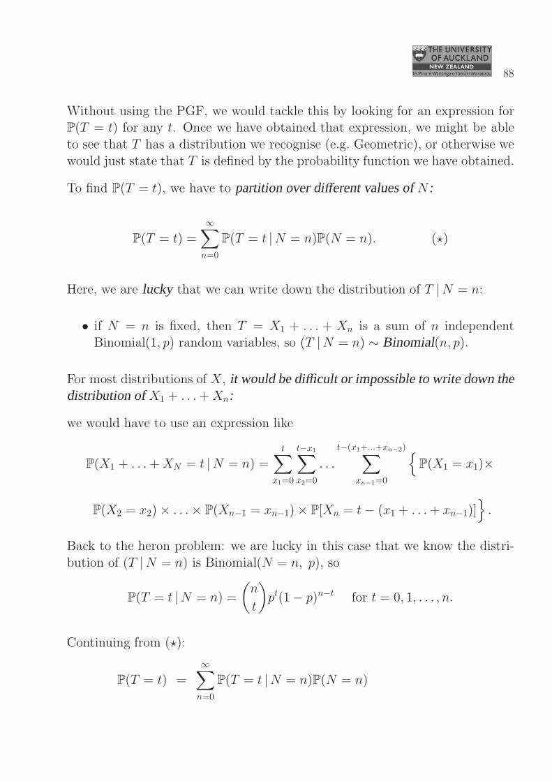
Without using the PGF, we would tackle this by looking for an expression forP(T = t) for any t. Once we have obtained that expression, we might be able
to see that T has a distribution we recognise (e.g. Geometric), or otherwise wewould just state that T is defined by the probability function we have obtained.
To find P(T = t), we have to partition over different values ofN :
P(T = t) =
∞∑
n=0
P(T = t |N = n)P(N = n). (⋆)
Here, we are lucky that we can write down the distribution of T |N = n:
• if N = n is fixed, then T = X1 + . . . + Xn is a sum of n independentBinomial(1, p) random variables, so (T |N = n) ∼ Binomial(n, p).
For most distributions of X, it would be difficult or impossible to write down thedistribution ofX1 + . . .+Xn:
we would have to use an expression like
P(X1 + . . .+XN = t |N = n) =t∑
x1=0
t−x1∑
x2=0
. . .
t−(x1+...+xn−2)∑
xn−1=0
{
P(X1 = x1)×
P(X2 = x2)× . . .× P(Xn−1 = xn−1)× P[Xn = t− (x1 + . . .+ xn−1)]}
.
Back to the heron problem: we are lucky in this case that we know the distri-
bution of (T |N = n) is Binomial(N = n, p), so
P(T = t |N = n) =
(
n
t
)
pt(1− p)n−t for t = 0, 1, . . . , n.
Continuing from (⋆):
P(T = t) =∞∑
n=0
P(T = t |N = n)P(N = n)
89
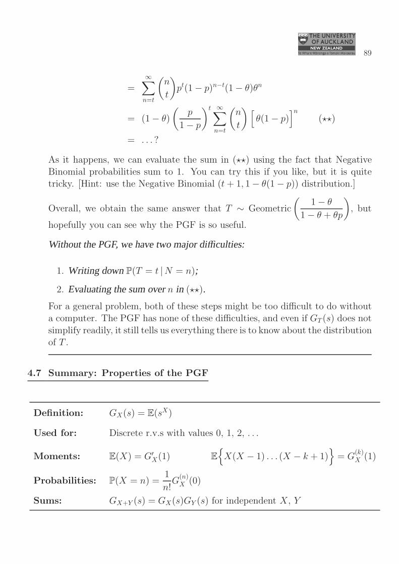
=∞∑
n=t
(
n
t
)
pt(1− p)n−t(1− θ)θn
= (1− θ)
(
p
1− p
)t ∞∑
n=t
(
n
t
)
[
θ(1− p)]n
(⋆⋆)
= . . . ?
As it happens, we can evaluate the sum in (⋆⋆) using the fact that Negative
Binomial probabilities sum to 1. You can try this if you like, but it is quitetricky. [Hint: use the Negative Binomial (t+ 1, 1− θ(1− p)) distribution.]
Overall, we obtain the same answer that T ∼ Geometric
(
1− θ
1− θ + θp
)
, but
hopefully you can see why the PGF is so useful.
Without the PGF, we have two major difficulties:
1. Writing downP(T = t |N = n);
2. Evaluating the sum overn in (⋆⋆).
For a general problem, both of these steps might be too difficult to do withouta computer. The PGF has none of these difficulties, and even if GT (s) does not
simplify readily, it still tells us everything there is to know about the distributionof T .
4.7 Summary: Properties of the PGF
Definition: GX(s) = E(sX)
Used for: Discrete r.v.s with values 0, 1, 2, . . .
Moments: E(X) = G′X(1) E
{
X(X − 1) . . . (X − k + 1)}
= G(k)X (1)
Probabilities: P(X = n) =1
n!G
(n)X (0)
Sums: GX+Y (s) = GX(s)GY (s) for independent X, Y
90
4.8 Convergence of PGFs
We have been using PGFs throughout this chapter without paying much at-tention to their mathematical properties. For example, are we sure that the
power series GX(s) =∑∞
x=0 sxP(X = x) converges? Can we differentiate and
integrate the infinite power series term by term as we did in Section 4.4? Whenwe said in Section 4.4 that E(X) = G′
X(1), can we be sure that GX(1) and its
derivative G′X(1) even exist?
This technical section introduces the radius of convergence of the PGF.Although it isn’t obvious, it is always safe to assume convergence of GX(s) at
least for |s| < 1. Also, there are results that assure us that E(X) = G′X(1) will
work for all non-defective random variables X.
Definition: The radius of convergence of a probability generating function is anumberR > 0, such that the sumGX(s) =
∑∞x=0 s
xP(X = x) converges if
|s| < R and diverges (→ ∞) if |s| > R.
(No general statement is made about what happens when |s| = R.)
Fact: For any PGF, the radius of convergence exists.
It is always ≥ 1: every PGF converges for at least s ∈ (−1, 1).
The radius of convergence could be anything from R = 1 to R = ∞.
Note: This gives us the surprising result that the set of s for which the PGF GX(s)
converges is symmetric about 0: the PGF converges for all s ∈ (−R,R), andfor no s < −R or s > R.
This is surprising because the PGF itself is not usually symmetric about 0: i.e.GX(−s) 6= GX(s) in general.
Example 1: Geometric distribution
Let X ∼ Geometric(p = 0.8). What is the radius of convergence of GX(s)?
91
As in Section 4.2,
GX(s) =∞∑
x=0
sx(0.8)(0.2)x = 0.8∞∑
x=0
(0.2s)x
=0.8
1− 0.2sfor all s such that|0.2s| < 1.
This is valid for alls with |0.2s| < 1, so it is valid for alls with |s| < 10.2 = 5.
(i.e.−5 < s < 5.)The radius of convergence isR = 5.
The figure shows the PGF of the Geometric(p = 0.8) distribution, with itsradius of convergence R = 5. Note that although the convergence set (−5, 5) is
symmetric about 0, the function GX(s) = p/(1− qs) = 4/(5− s) is not.
−5 0 5
01
23
45
G(s)
s
to infinity
Radius of Convergence
Geometric(0.8) probability generating function
but it is no longer equal to E(s ).In this region, p/(1−qs) remains finite and well−behaved,
X
At the limits of convergence, strange things happen:
• At the positive end, as s ↑ 5, both GX(s) and p/(1− qs) approach infinity.So the PGF is (left)-continuous at +R:
lims↑5
GX(s) = GX(5) = ∞.
However, the PGF does not converge at s = +R.
92
• At the negative end, as s ↓ −5, the function p/(1 − qs) = 4/(5 − s) iscontinuous and passes through 0.4 when s = −5. However, when s ≤−5, this function no longer represents GX(s) = 0.8
∑∞x=0(0.2s)
x, because|0.2s| ≥ 1.
Additionally, when s = −5, GX(−5) = 0.8∑∞
x=0(−1)x does not exist.Unlike the positive end, this means that GX(s) is not (right)-continuous
at −R:lims↓−5
GX(s) = 0.4 6= GX(−5).
Like the positive end, this PGF does not converge at s = −R.
Example 2: Binomial distribution
Let X ∼ Binomial(n, p). What is the radius of convergence of GX(s)?
As in Section 4.2,
GX(s) =n∑
x=0
sx(
n
x
)
pxqn−x
=n∑
x=0
(
n
x
)
(ps)xqn−x
= (ps+ q)n by the Binomial Theorem: true for alls.
This is true for all−∞ < s < ∞, so the radius of convergence isR = ∞.
Abel’s Theorem for continuity of power series at s = 1
Recall from above that if X ∼ Geometric(0.8), then GX(s) is not continuousat the negative end of its convergence (−R):
lims↓−5
GX(s) 6= GX(−5).
Abel’s theorem states that this sort of effect can never happen at s = 1 (or at
+R). In particular, GX(s) is always left-continuous at s = 1:
lims↑1
GX(s) = GX(1) always, even if GX(1) = ∞.
93
Theorem 4.8: Abel’s Theorem.
Let G(s) =
∞∑
i=0
pisi for any p0, p1, p2, . . . with pi ≥ 0 for all i.
Then G(s) is left-continuous at s = 1:
lims↑1
G(s) =∞∑
i=0
pi = G(1) ,
whether or not this sum is finite.
Note: Remember that the radius of convergence R ≥ 1 for any PGF, so Abel’sTheorem means that even in the worst-case scenario when R = 1, we can still
trust that the PGF will be continuous at s = 1. (By contrast, we can not besure that the PGF will be continuous at the the lower limit −R).
Abel’s Theorem means that for any PGF, we can write GX(1) as shorthand forlims↑1GX(s).
It also clarifies our proof that E(X) = G′X(1) from Section 4.4. If we assume
that term-by-term differentiation is allowed for GX(s) (see below), then theproof on page 81 gives:
GX(s) =∞∑
x=0
sx px,
so G′X(s) =
∞∑
x=1
xsx−1px (term-by-term differentiation: see below).
Abel’s Theorem establishes that E(X) is equal to lims↑1G′X(s):
E(X) =∞∑
x=1
xpx
= G′X(1)
= lims↑1
G′X(s),
because Abel’s Theorem applies to G′X(s) =
∑∞x=1 xs
x−1px, establishing thatG′
X(s) is left-continuous at s = 1. Without Abel’s Theorem, we could not be
sure that the limit of G′X(s) as s ↑ 1 would give us the correct answer for E(X).
94
Absolute and uniform convergence for term-by-term differentiation
We have stated that the PGF converges for all |s| < R for some R. In fact,
the probability generating function converges absolutely if |s| < R. Absoluteconvergence is stronger than convergence alone: it means that the sum of abso-
lute values,∑∞
x=0 |sxP(X = x)|, also converges. When two series both convergeabsolutely, the product series also converges absolutely. This guarantees that
GX(s)×GY (s) is absolutely convergent for any two random variables X and Y .This is useful because GX(s)×GY (s) = GX+Y (s) if X and Y are independent.
The PGF also converges uniformly on any set {s : |s| ≤ R′} where R′ < R.Intuitively, this means that the speed of convergence does not depend upon the
value of s. Thus a value n0 can be found such that for all values of n ≥ n0,the finite sum
∑nx=0 s
xP(X = x) is simultaneously close to the converged value
GX(s), for all s with |s| ≤ R′. In mathematical notation: ∀ǫ > 0, ∃n0 ∈Z such that ∀s with |s| ≤ R′, and ∀n ≥ n0,
∣
∣
∣
∣
∣
n∑
x=0
sxP(X = x)−GX(s)
∣
∣
∣
∣
∣
< ǫ.
Uniform convergence allows us to differentiate or integrate the PGF term by
term.
Fact: Let GX(s) = E(sX) =∑∞
x=0 sxP(X = x), and let s < R.
1. G′X(s)=
d
ds
( ∞∑
x=0
sxP(X = x)
)
=
∞∑
x=0
d
ds(sxP(X = x))=
∞∑
x=0
xsx−1P(X = x).
(term by term differentiation).
2.
∫ b
a
GX(s) ds =
∫ b
a
( ∞∑
x=0
sxP(X = x)
)
ds =
∞∑
x=0
(∫ b
a
sxP(X = x) ds
)
=∞∑
x=0
sx+1
x+ 1P(X = x) for −R < a < b < R.
(term by term integration).
95
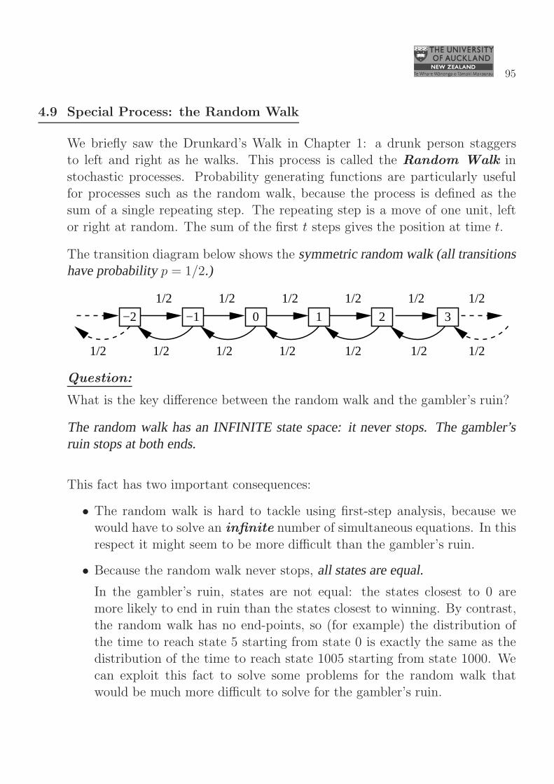
4.9 Special Process: the Random Walk
We briefly saw the Drunkard’s Walk in Chapter 1: a drunk person staggersto left and right as he walks. This process is called the Random Walk in
stochastic processes. Probability generating functions are particularly usefulfor processes such as the random walk, because the process is defined as thesum of a single repeating step. The repeating step is a move of one unit, left
or right at random. The sum of the first t steps gives the position at time t.
The transition diagram below shows the symmetric random walk (all transitionshave probabilityp = 1/2.)
1/2
1/2
2 3
1/2
1/2 1/2
−2
1/2
1/2
0
1/2
1/2
−1
1/2
1/2
1
1/2
1/2
Question:
What is the key difference between the random walk and the gambler’s ruin?
The random walk has an INFINITE state space: it never stops. The gambler’sruin stops at both ends.
This fact has two important consequences:
• The random walk is hard to tackle using first-step analysis, because wewould have to solve an infinite number of simultaneous equations. In this
respect it might seem to be more difficult than the gambler’s ruin.
• Because the random walk never stops, all states are equal.
In the gambler’s ruin, states are not equal: the states closest to 0 are
more likely to end in ruin than the states closest to winning. By contrast,the random walk has no end-points, so (for example) the distribution of
the time to reach state 5 starting from state 0 is exactly the same as thedistribution of the time to reach state 1005 starting from state 1000. We
can exploit this fact to solve some problems for the random walk thatwould be much more difficult to solve for the gambler’s ruin.
96
PGFs for finding the distribution of reaching times
For random walks, we are particularly interested in reaching times:
• How long will it take us to reach state j, starting from state i?
• Is there a chance that we will never reach state j, starting from state i?
In Chapter 3 we saw how to find expected reaching times: the expectednumber of steps taken to reach a particular state. We used the law of totalexpectation and first-step analysis (Section 3.5).
However, the expected or average reaching time doesn’t tell the whole story.Think back to the model for gene spread in Section 3.7. If there is just oneanimal out of 100 with the harmful allele, the expected number of generations to
fixation is quite large at 10.5: even though the allele will usually die out after oneor two generations. The high average is caused by a small chance that the allele
will take hold and grow, requiring a very large number of generations before iteither dies out or saturates the population. In most stochastic processes, the
average is of limited use by itself, without having some idea about the varianceand skew of the distribution.
With our tool of PGFs, we can characterise the whole distribution of the timeT taken to reach a particular state, by finding its PGF. This will give us the
mean, variance, and skew by differentiation. In principle the PGF could evengive us the full set of probabilities, P(T = t) for all possible t = 0, 1, 2, . . .,
though in practice it may be computationally infeasible to find more than thefirst few probabilities by repeated differentiation.
However, there is a new and very useful piece of information that the PGF can
tell us quickly and easily:
what is the probability that we NEVER reach statej, starting from statei?
For example, imagine that the random walk represents the share value for an
investment. The current share price is i dollars, and we might decide to sellwhen it reaches j dollars. Knowing how long this might take, and whether there
is a chance we will never succeed, is fundamental to managing our investment.
97
To tackle this problem, we define the random variable T to be the time taken(number of steps) to reach state j, starting from state i. We find the PGF of
T , and then use the PGF to discover P(T = ∞). If P(T = ∞) > 0, there is apositive chance that we will NEVER reach state j, starting from state i.
We will see how to determine the probability of never reaching our goal in
Section 4.11. First we will see how to calculate the PGF of a reaching time Tin the random walk.
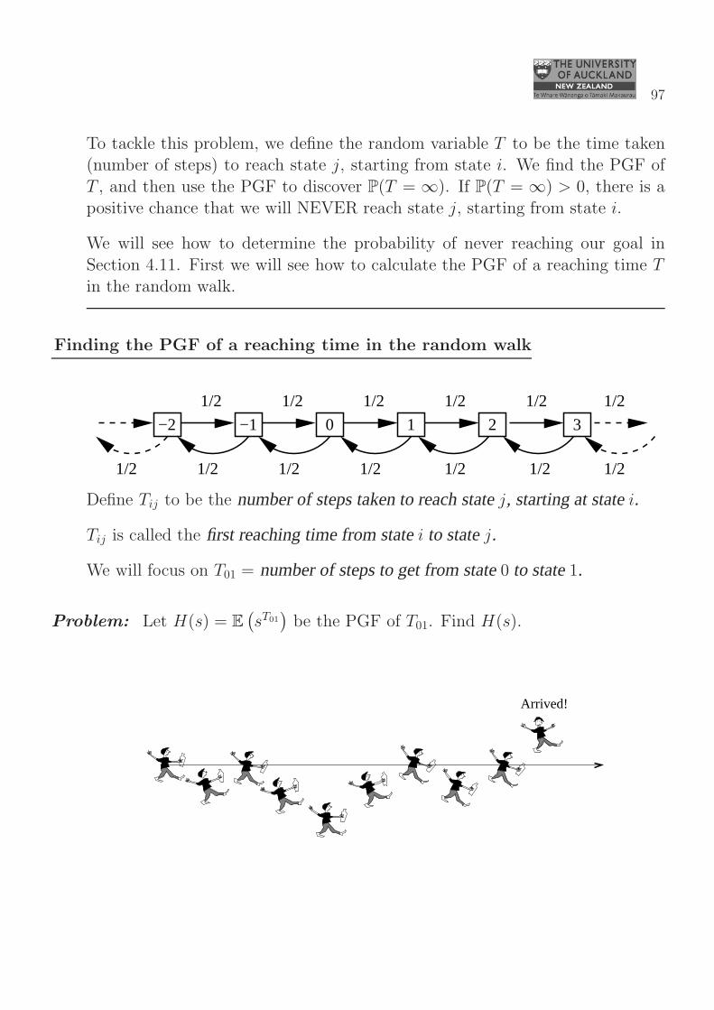
Finding the PGF of a reaching time in the random walk
1/2
1/2
2 3
1/2
1/2 1/2
−2
1/2
1/2
0
1/2
1/2
−1
1/2
1/2
1
1/2
1/2
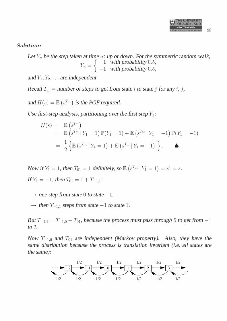
Define Tij to be the number of steps taken to reach statej, starting at statei.
Tij is called the first reaching time from statei to statej.
We will focus on T01 = number of steps to get from state0 to state1.
Problem: Let H(s) = E(
sT01
)
be the PGF of T01. Find H(s).
Arrived!
98
Solution:
Let Yn be the step taken at timen: up or down. For the symmetric random walk,
Yn =
{
1 with probability0.5,−1 with probability0.5,
andY1, Y2, . . . are independent.
RecallTij = number of steps to get from statei to statej for anyi, j,
andH(s) = E(
sT01
)
is the PGF required.
Use first-step analysis, partitioning over the first stepY1:
H(s) = E(
sT01
)
= E(
sT01 |Y1 = 1)
P(Y1 = 1) + E(
sT01 |Y1 = −1)
P(Y1 = −1)
=1
2
{
E(
sT01 |Y1 = 1)
+ E(
sT01 |Y1 = −1)
}
. ♠
Now if Y1 = 1, thenT01 = 1 definitely, soE(
sT01 |Y1 = 1)
= s1 = s.
If Y1 = −1, thenT01 = 1 + T−1,1:
→ one step from state0 to state−1,
→ thenT−1,1 steps from state−1 to state1.
But T−1,1 = T−1,0 + T01, because the process must pass through 0 to get from−1
to 1.
Now T−1,0 and T01 are independent (Markov property). Also, they have thesame distribution because the process is translation invariant (i.e. all states arethe same):
1/2
1/2
2 3
1/2
1/2 1/2
−2
1/2
1/2
0
1/2
1/2
−1
1/2
1/2
1
1/2
1/2
99
Thus
E(
sT01 |Y1 = −1)
= E(
s1+T−1,1)
= E(
s1+T−1,0+T0,1)
= sE(
sT−1,0)
E(
sT01
)
by independence= s(H(s))2 because identically distributed.
ThusH(s) =
1
2
{
s+ s(H(s))2}
by ♠.
This is a quadratic inH(s):1
2s(H(s))2 −H(s) +
1
2s = 0
⇒ H(s) =1±
√
1− 412s
12s
s=
1±√1− s2
s.
Which root? We know thatP(T01 = 0) = 0, because it must take at least one step
to go from 0 to 1. With the positive root,lims→0H(0) = lims→0
(
2
s
)
= ∞; so
we take the negative root instead.
Thus H(s) =1−
√1− s2
s.
Check this haslims→0H(s) = 0 by L’Hospital’s Rule:
lims→0
(
f(s)
g(s)
)
= lims→0
(
f ′(s)
g′(s)
)
= lims→0
{
12(1− s2)−1/2 × 2s
1
}
= 0.
100
Notation for quick solutions of first-step analysis for finding PGFs
As with first-step analysis for finding hitting probabilities and expected reachingtimes, setting up a good notation is extremely important. Here is a goodnotation for finding H(s) = E
(
sT01
)
.
Let T = T01. SeekH(s) = E(sT ).
Now
T =
{
1 with probability1/2,
1 + T ′ + T ′′ with probability1/2,
whereT ′ ∼ T ′′ ∼ T andT ′, T ′′ are independent.
Taking expectations:
H(s) = E(sT ) =
{
E(
s1)
w. p. 1/2
E(
s1+T ′+T ′′)
w. p. 1/2
⇒ H(s) =
{
s w. p. 1/2
sE(
sT′)
E(
sT′′)
w. p. 1/2 (by independence ofT ′ andT ′′)
⇒ H(s) =
{
s w. p. 1/2
sH(s)H(s) w. p. 1/2 (becauseT ′ ∼ T ′′ ∼ T )
⇒ H(s) = 12s+ 1
2sH(s)2.
101
Thus:sH(s)2 − 2H(s) + s = 0.
Solve the quadratic and select the correct root as before, toget
H(s) =1−
√1− s2
sfor |s| < 1.
4.10 Defective random variables
A random variable is said to be defective if it can take the value∞.
In stochastic processes, a reaching timeTij is defective if there is a chance thatwe NEVER reach statej, starting from statei.
The probability that we never reach state j, starting from state i, is the same
as the probability that the time taken is infinite: Tij = ∞:
P(Tij = ∞) = P(we NEVER reach statej, starting from statei).
In other cases, we will alwaysreach statej eventually, starting from statei.
In that case, Tij can nottake the value∞:
P(Tij = ∞) = 0 if we are CERTAIN to reach statej, starting from statei.
Definition: A random variable T is defective, or improper, if it can take the value∞. That is,
T is defective if P(T = ∞) > 0.
102
Thinking of∑
∞
t=0P(T = t) as 1 − P(T = ∞)
Although it seems strange, when we write∑∞
t=0 P(T = t), we are notincludingthe valuet = ∞.
The sum∑∞
t=0 continues without ever stopping: at no point can we say we have
‘finished’ all the finite values of t so we will now add on t = ∞. We simplynever get tot = ∞ when we take
∑∞t=0.
For a defective random variable T , this means that
∞∑
t=0
P(T = t) < 1,
because we are missing the positive value of P(T = ∞).
All probabilities of T must still sum to 1, so we have
1 =
∞∑
t=0
P(T = t) + P(T = ∞),
in other words ∞∑
t=0
P(T = t) = 1− P(T = ∞).
PGFs for defective random variables
When T is defective, the PGF of T is defined as the power series
H(s) =∞∑
t=0
P(T = t)st for |s| < 1.
The term for P(T = ∞)s∞ is missed out. The PGF is defined as the generatingfunction of the probabilities for finite values only.
103
Because H(s) is a power series satisfying the conditions of Abel’s Theorem, weknow that:
• H(s) is left-continuous at s = 1, i.e. lims↑1H(s) = H(1).
This is different from the behaviour of E(sT ), if T is defective:
• E(sT ) = H(s) for |s| < 1 because the missing term is zero: i.e. because
s∞ = 0 when |s| < 1.
• E(sT ) is NOT left-continuous at s = 1. There is a sudden leap (disconti-nuity) at s = 1 because s∞ = 0 as s ↑ 1, but s∞ = 1 when s = 1.
Thus H(s) does NOT represent E(sT ) at s = 1. It is as if H(s) is a ‘train’ thatE(sT ) rides on between −1 < s < 1. At s = 1, the train keeps going (i.e. H(s)
is continuous) but E(sT ) jumps off the train.
We test whether T is defective by testing whether or not E(sT ) ‘jumps off thetrain’ — that is, we test whether or not H(s) is equal to E(sT ) when s = 1.
We know what E(sT ) is when s = 1:
• E(sT ) is always 1 when s = 1, whether T is defective or not:
E(1T ) = 1 for ANY random variable T .
But the function H(s) =∑∞
t=0 stP(T = t) may or may not be 1 when s = 1:
• If T is defective, H(s) is missing a term and H(1) < 1.
• If T is not defective, H(s) is not missing anything so H(1) = 1.
Test for defectiveness:
Let H(s) =∑∞
t=0 stP(T = t) be the power series representing the PGF of T
for |s| < 1. Then T is defective if and only if H(1) < 1.
104
Using defectiveness to find the probability we never get there
The simple test for defectiveness tells us whether there is a positive probabilitythat we NEVER reach our goal. Here are the steps.
1. We want to know the probability that we will NEVER reach state j, start-ing from state i.
2. Define T to be the random variable giving the number of steps taken toget from state i to state j.
3. The event that we never reach state j, starting from state i, is the sameas the event that T = ∞. (If we wait an infinite length of time, we never
get there.) So
P(never reach statej | start at statei) = P(T = ∞).
4. Find H(s) =∑∞
t=0 stP(T = t), using a calculation like the one we did in
Section 4.9. H(s) is the PGF of T for |s| < 1. We only need to find it for|s| < 1. The calculation in Section 4.9 only works for |s| ≤ 1 because the
expectations are infinite or undefined when |s| > 1.
5. The random variable T is defective if and only if H(1) < 1.
6. If H(1) < 1, then the probability that T takes the value ∞ is the missingpiece: P(T = ∞) = 1−H(1).
Overall:
P( never reach statej | start at statei) = P(T = ∞) = 1−H(1).
Expectation and variance of a defective random variable
If T is defective, there is a positive chance that T = ∞. This means thatE(T ) = ∞, Var(T ) = ∞, andE(T a) = ∞ for any powera.
105
E(T ) and Var(T ) can not be found using the PGF when T is defective: youwill get the wrong answer.
When you are asked to find E(T ) in a context where T might be defective:
• First check whether T is defective: is H(1) < 1 or= 1?
• If T is defective, then E(T ) = ∞.
• If T is not defective (H(1) = 1), then E(T ) = H ′(1) as usual.
4.11 Random Walk: the probability we never reach our goal
In the random walk in Section 4.9, we defined the first reaching time T01 as the
number of steps taken to get from state 0 to state 1.
In Section 4.9 we found the PGF of T01 to be:
PGF ofT01 = H(s) =1−
√1− s2
sfor |s| < 1.
Questions:
a) What is the probability that we never reach state 1, starting from state 0?
b) What is expected number of steps to reach state 1, starting from state 0?
Solutions:
a) We need to know whetherT01 is defective.
T01 is defective if and only ifH(1) < 1.
Now H(1) = 1−√1−12
1= 1. SoT01 is notdefective.
ThusP(never reach state 1| start from state 0) = 0.
We will DEFINITELY reach state 1 eventually, even if it takesa very long time.
106
b) BecauseT01 is not defective, we can findE(T01) by differentiating the PGF:E(T01) = H ′(1).
H(s) =1−
√1− s2
s= s−1 −
(
s−2 − 1)1/2
So H ′(s) = −s−2 − 1
2
(
s−2 − 1)−1/2 (−2s−3
)
Thus
E(T01) = lims↑1
H ′(s) = lims↑1
− 1
s2+
1
s3√
1s2 − 1
= ∞.
So the expected number of steps to reach state 1 starting fromstate 0 is infinite:E(T01) = ∞.
This result is striking. Even though we will definitely reach state 1, the
expected time to do so is infinite! In general, we can prove the following resultsfor random walks, starting from state 0:
0
p
1
q
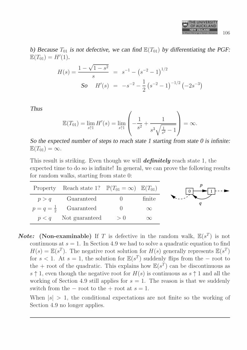
Property Reach state 1? P(T01 = ∞) E(T01)
p > q Guaranteed 0 finite
p = q = 12 Guaranteed 0 ∞
p < q Not guaranteed > 0 ∞
Note: (Non-examinable) If T is defective in the random walk, E(sT ) is notcontinuous at s = 1. In Section 4.9 we had to solve a quadratic equation to find
H(s) = E(sT ). The negative root solution for H(s) generally represents E(sT )for s < 1. At s = 1, the solution for E(sT ) suddenly flips from the − root tothe + root of the quadratic. This explains how E(sT ) can be discontinuous as
s ↑ 1, even though the negative root for H(s) is continuous as s ↑ 1 and all theworking of Section 4.9 still applies for s = 1. The reason is that we suddenly
switch from the − root to the + root at s = 1.
When |s| > 1, the conditional expectations are not finite so the working of
Section 4.9 no longer applies.