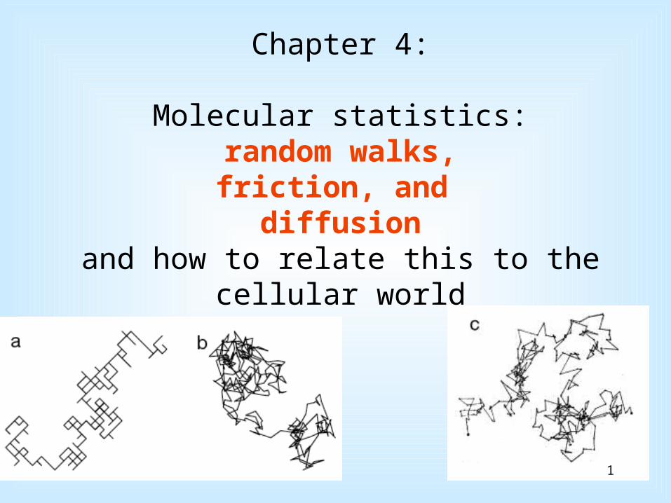
Chapter 4:

Molecular statistics: random walks,

friction, and diffusion

and how to relate this to the cellular world

1

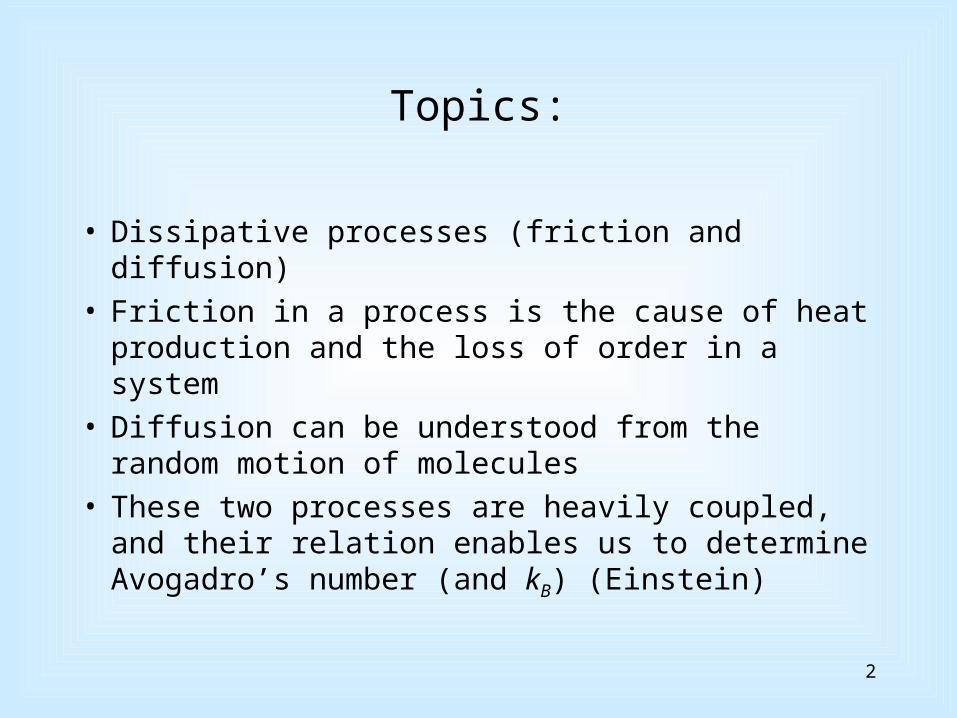
Topics:

• Dissipative processes (friction and diffusion)• Friction in a process is the cause of heat

production and the loss of order in a system• Diffusion can be understood from the random

motion of molecules• These two processes are heavily coupled, and their

relation enables us to determine Avogadro’s number (and kB) (Einstein)

2

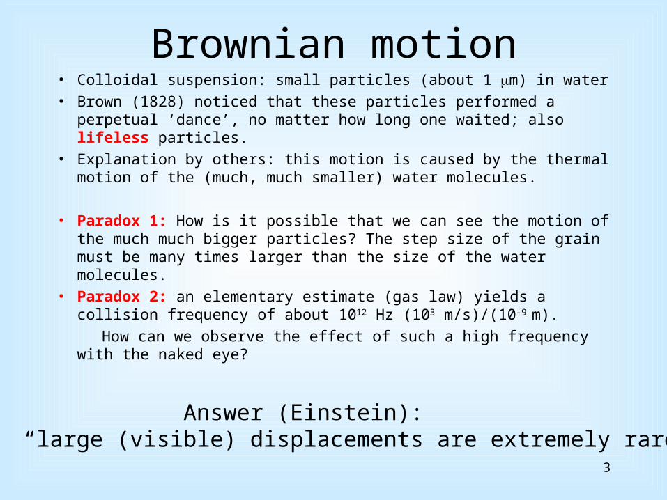
Brownian motion• Colloidal suspension: small particles (about 1 m) in water

• Brown (1828) noticed that these particles performed a perpetual ‘dance’, no matter how long one waited; also lifeless particles.

• Explanation by others: this motion is caused by the thermal motion of the (much, much smaller) water molecules.

• Paradox 1: How is it possible that we can see the motion of the much much bigger particles? The step size of the grain must be many times larger than the size of the water molecules.

• Paradox 2: an elementary estimate (gas law) yields a collision frequency of about 1012 Hz (103 m/s)/(10-9 m).

How can we observe the effect of such a high frequency with the naked eye?

3

Answer (Einstein): “large (visible) displacements are extremely rare!”

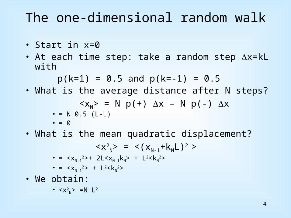
The one-dimensional random walk

• Start in x=0• At each time step: take a random step x=kL with p(k=1) = 0.5 and p(k=-1) = 0.5• What is the average distance after N steps?

<xN> = N p(+) x – N p(-) x • = N 0.5 (L-L)• = 0

• What is the mean quadratic displacement?

<x2N> = <(xN-1+kNL)2 >

• = <xN-12>+ 2L<xN-1kN> + L2<kN

2>• = <xN-1

2> + L2<kN2>

• We obtain:• <x2

N> =N L2

4

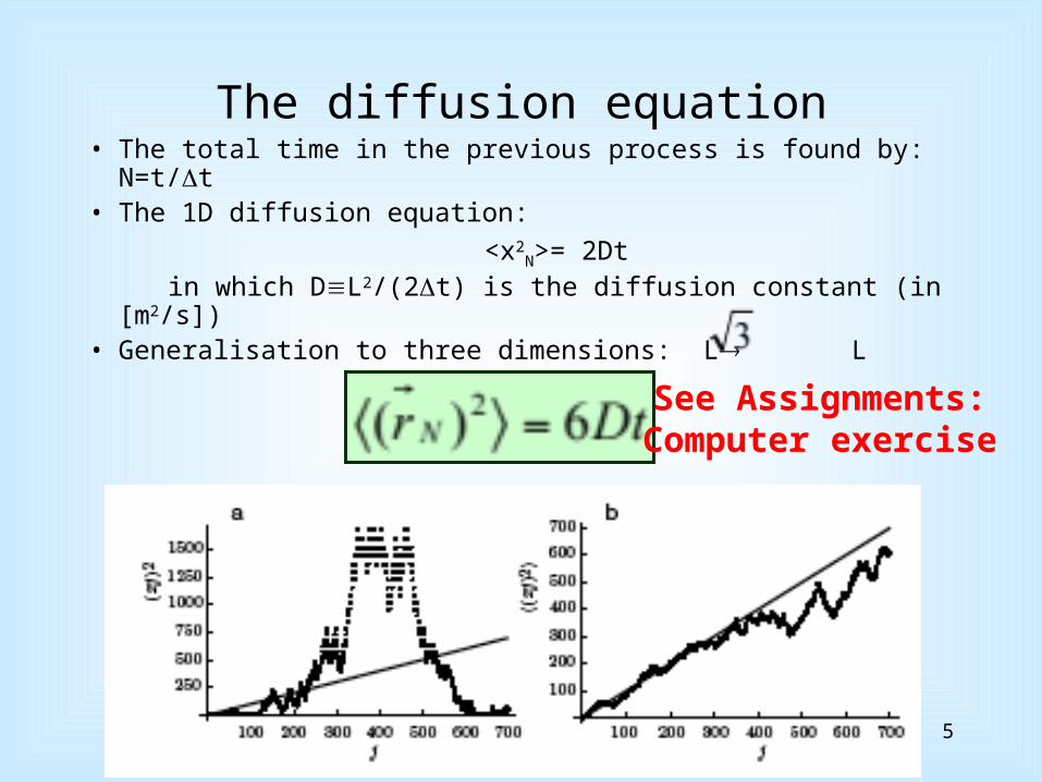
The diffusion equation• The total time in the previous process is found by: N=t/t• The 1D diffusion equation:

<x2N>= 2Dt

in which DL2/(2t) is the diffusion constant (in [m2/s])• Generalisation to three dimensions: L L

5

See Assignments:Computer exercise

Diffusion is a random process

• The paradox of small displacements and high frequencies is resolved because we can only observe the effect of very large displacements. These have a very low probability, and therefore occur at a very low frequency!

• The diffusion equation does not depend on the distribution of step sizes (You are going to show this in the computer exercise!)

• Diffusion is a collective random walk of many particles• The position-probability distribution becomes observable as a particle

density profile

6

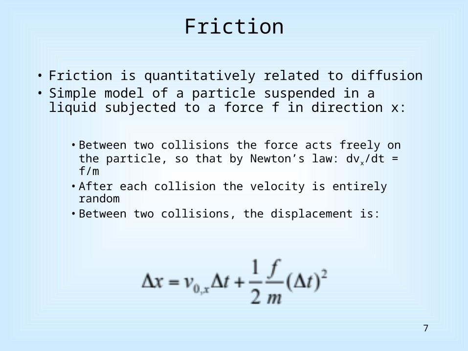
Friction

• Friction is quantitatively related to diffusion• Simple model of a particle suspended in a liquid

subjected to a force f in direction x:

• Between two collisions the force acts freely on the particle, so that by Newton’s law: dvx/dt = f/m

• After each collision the velocity is entirely random • Between two collisions, the displacement is:

7

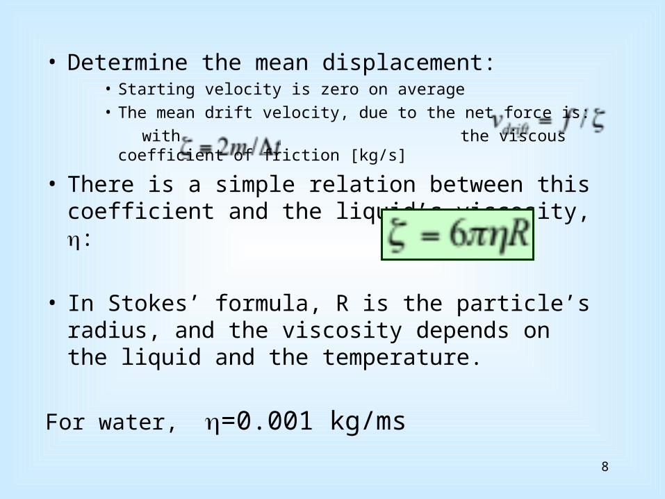
• Determine the mean displacement:

• Starting velocity is zero on average

• The mean drift velocity, due to the net force is:

with the viscous coefficient of friction [kg/s]

• There is a simple relation between this coefficient and the liquid’s viscosity, :

• In Stokes’ formula, R is the particle’s radius, and the viscosity depends on the liquid and the temperature.

For water, =0.001 kg/ms

8

The Einstein-relation

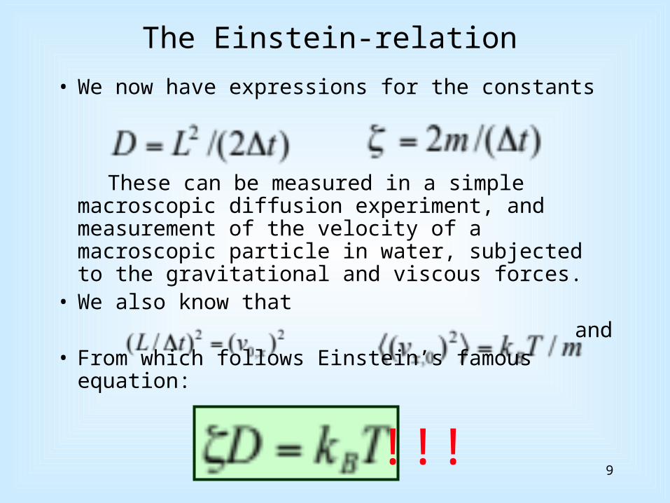
• We now have expressions for the constants

These can be measured in a simple macroscopic diffusion experiment, and measurement of the velocity of a macroscopic particle in water, subjected to the gravitational and viscous forces.

• We also know that and • From which follows Einstein’s famous equation:

9!!!

Finally, Avogadro’s number NA

• Take a thermometer and measure T• Measure the diffusion constant, D• Determine the friction coefficient, • Compute kB • Apply the ideal gas law and find NA

Note: Einstein’s equation is universal! It does not depend on the type of particle or liquid (although and

D do in a very complicated way!)

10

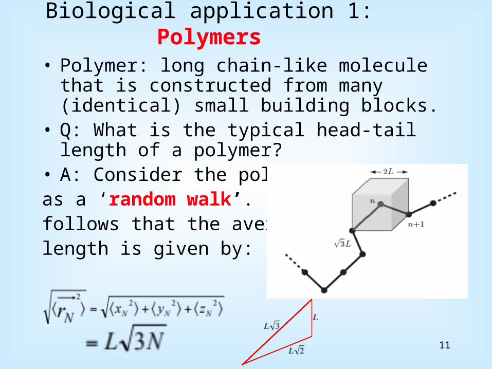
Biological application 1: Polymers

• Polymer: long chain-like molecule that is constructed from many (identical) small building blocks.

• Q: What is the typical head-tail length of a polymer?

• A: Consider the polymer as a ‘random walk’. It then follows that the averagelength is given by:

11

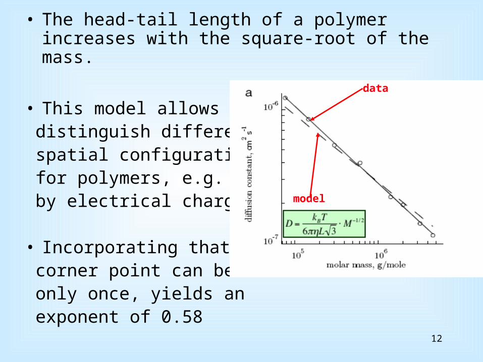
• The head-tail length of a polymer increases with the square-root of the mass.

• This model allows to distinguish different spatial configurations for polymers, e.g. caused by electrical charges.

• Incorporating that each corner point can be used only once, yields an exponent of 0.58

data

model

12

Diffusion: density profiles

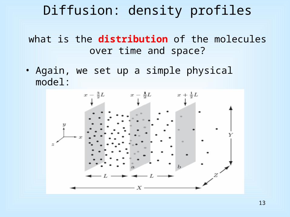
what is the distribution of the molecules over time and space?

• Again, we set up a simple physical model:

13

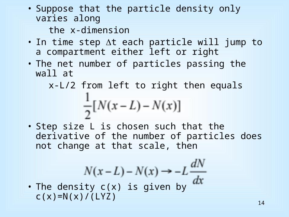
• Suppose that the particle density only varies along the x-dimension • In time step t each particle will jump to a

compartment either left or right • The net number of particles passing the wall at x-L/2 from left to right then equals

• Step size L is chosen such that the derivative of the number of particles does not change at that scale, then

• The density c(x) is given by c(x)=N(x)/(LYZ)14

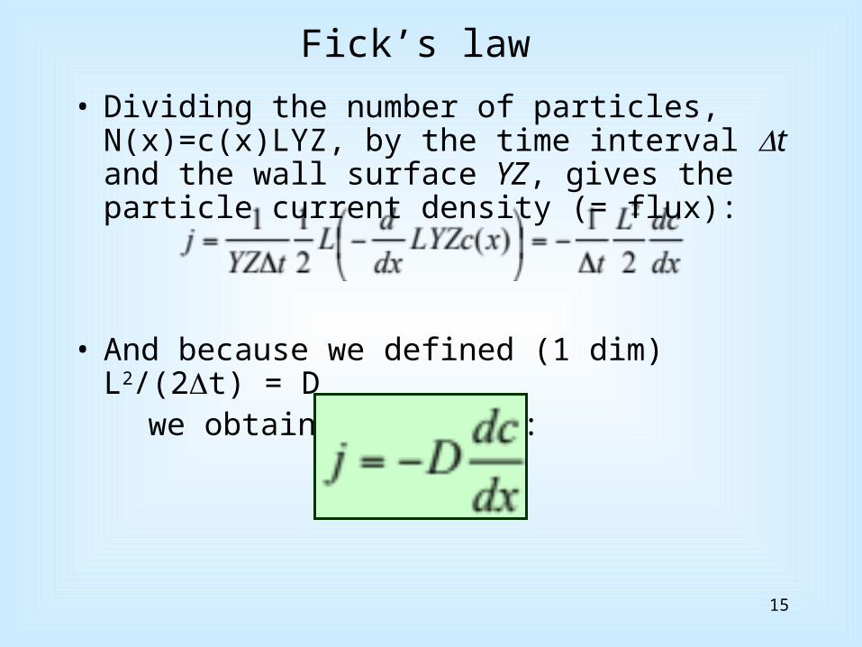
Fick’s law • Dividing the number of particles, N(x)=c(x)LYZ,

by the time interval t and the wall surface YZ, gives the particle current density (= flux):

• And because we defined (1 dim) L2/(2t) = D we obtain Fick’s law:

15

The diffusion equation

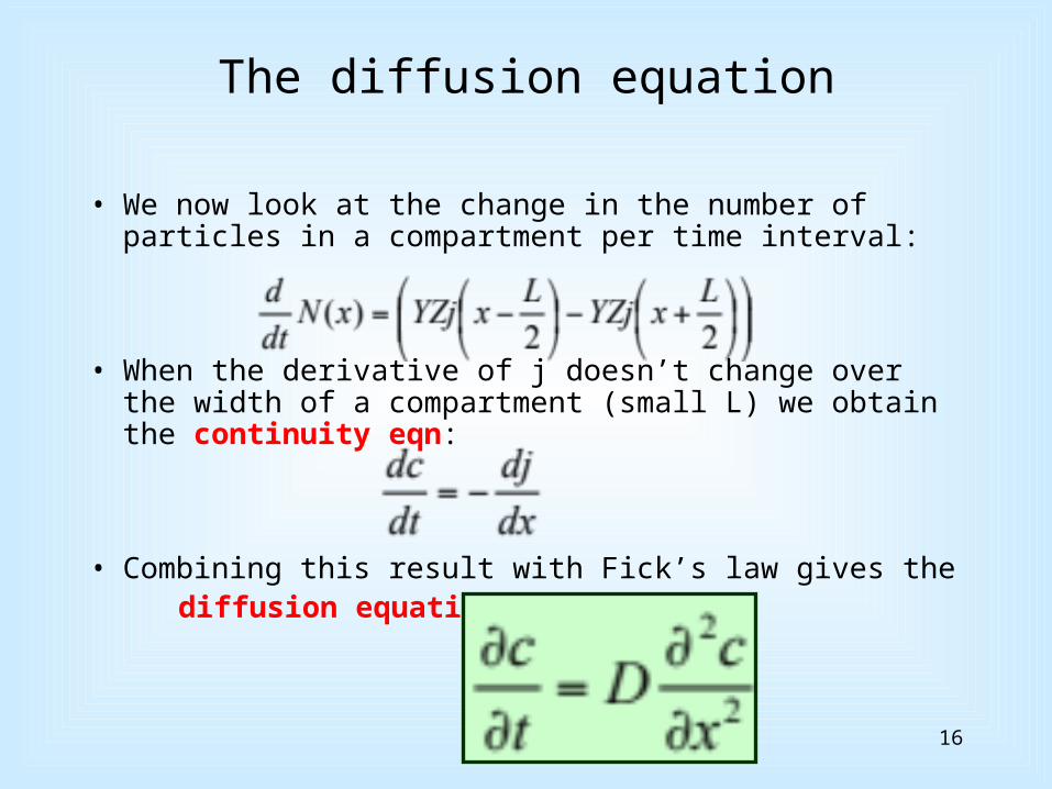
• We now look at the change in the number of particles in a compartment per time interval:

• When the derivative of j doesn’t change over the width of a compartment (small L) we obtain the continuity eqn:

• Combining this result with Fick’s law gives the diffusion equation:

16

Remarks:

• The diffusion equation describes Brownian motion for a large number of particles.

• For a large number of particles, the local probability to encounter a particle is represented by the density.

• The density evolves in a deterministic way according to the diffusion equation.

• When the number of particles is not large, the statistical approach is not accurate enough, because of the large influence of statistical fluctuations.

17

Diffusion through a thin tube

• A thin tube, length L, connects two basins with ink solution at different concentrations, c1 en c2

• The tube does not affect c1 and c2 • A constant concentration profile develops: Equilibrium: dc/dt=0, so d2c/dx2=0 Solve diffusion eqn.: c(x)=c1+(c2-c1)x/L Current density: j = -D(c)/L

18

Membrane permeability

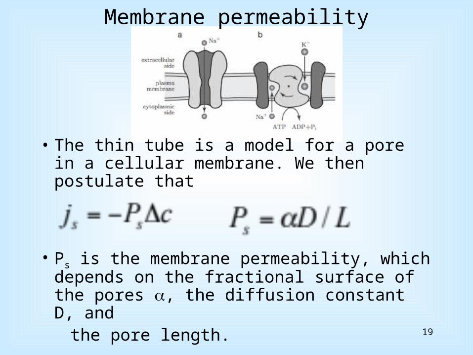
• The thin tube is a model for a pore in a cellular membrane. We then postulate that

• Ps is the membrane permeability, which depends on the fractional surface of the pores , the diffusion constant D, and

the pore length. 19

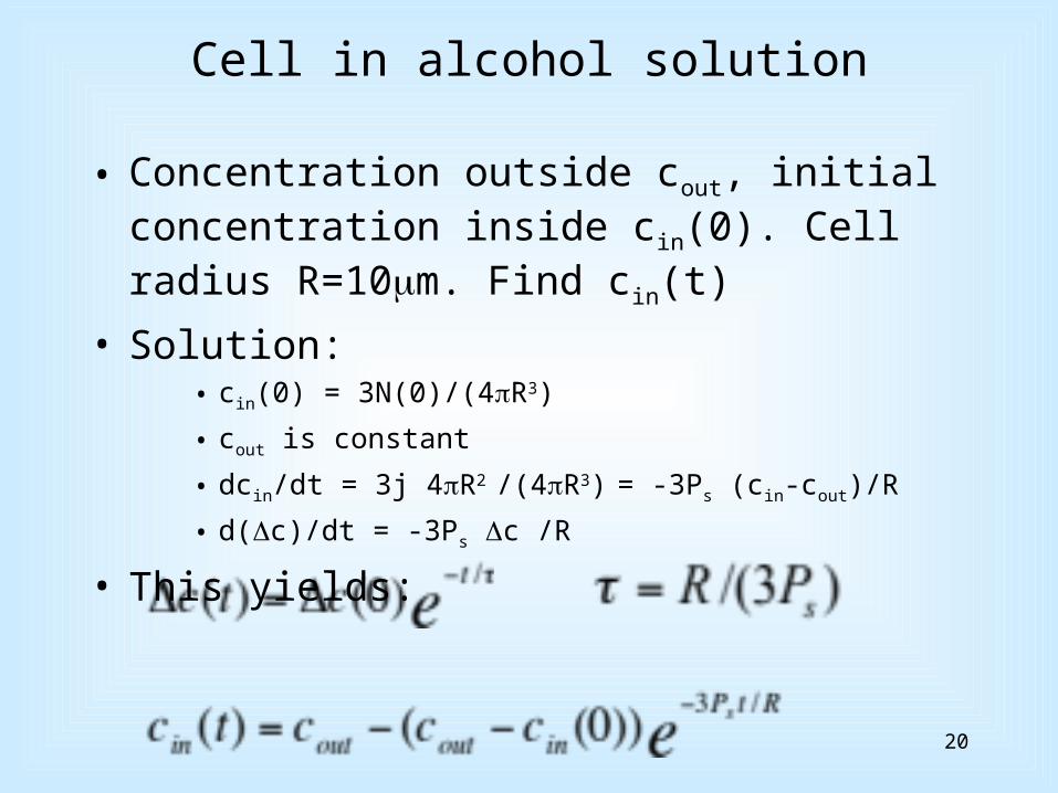
Cell in alcohol solution

• Concentration outside cout, initial concentration inside cin(0). Cell radius R=10m. Find cin(t)

• Solution: • cin(0) = 3N(0)/(4R3)

• cout is constant

• dcin/dt = 3j 4R2 /(4R3) = -3Ps (cin-cout)/R

• d(c)/dt = -3Ps c /R

• This yields:

20

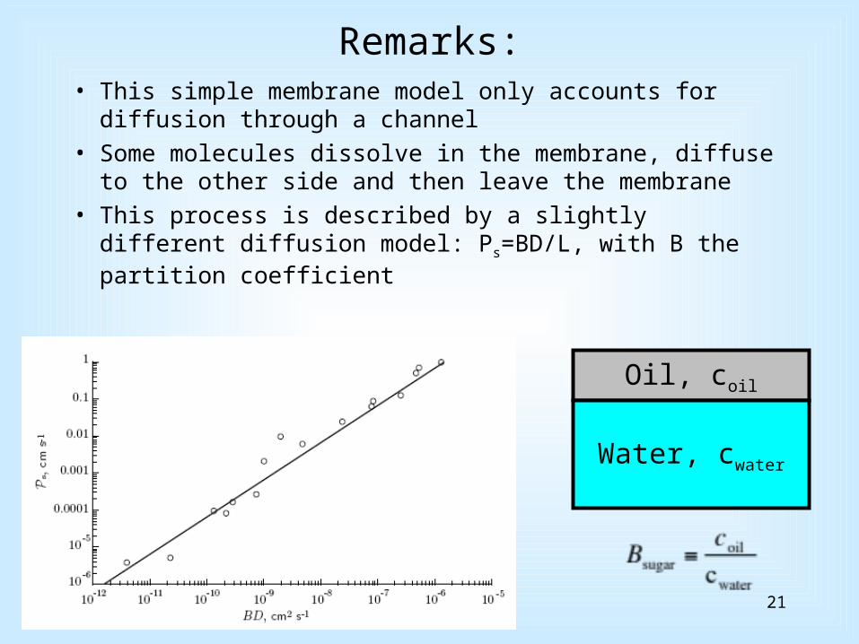
Remarks:• This simple membrane model only accounts for diffusion

through a channel

• Some molecules dissolve in the membrane, diffuse to the other side and then leave the membrane

• This process is described by a slightly different diffusion model: Ps=BD/L, with B the partition coefficient

Oil, coil

Water, cwater

21

Bacterial metabolism (= your turn….)

• What is the largest possible oxygen consumption of a bacterium (sphere, radius R) in water with oxygen concentration c0?

• Assume: stationary concentration profile

with c() = c0 en c(R) = 0• Inward flux j=D(dc/dr), and also j=I/(4r2)• This yields: c(r) =A-(1/r)(I/4D) • Apply boundary conditions: A=c0 en I=4DRc0

• c(r) = c0(1-R/r)• The maximal influx is proportional to R, but the

consumption to R3. This limits the maximum volume of a(ny!) bacterium! [see YT 4F]

22

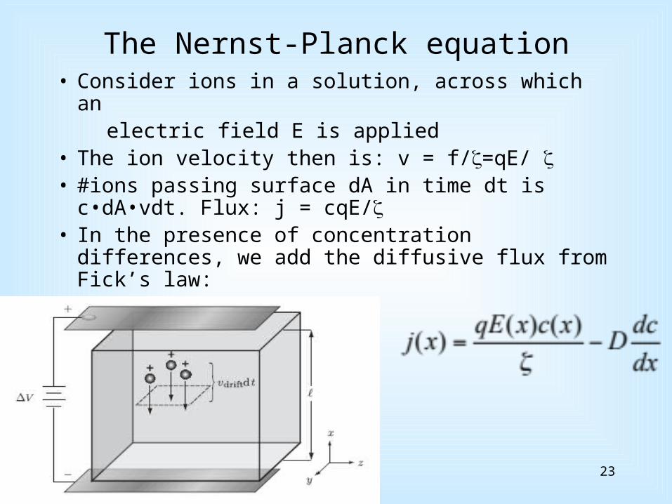
The Nernst-Planck equation• Consider ions in a solution, across which an electric field E is applied• The ion velocity then is: v = f/=qE/ • #ions passing surface dA in time dt is c•dA•vdt.

Flux: j = cqE/ • In the presence of concentration differences, we

add the diffusive flux from Fick’s law:

23

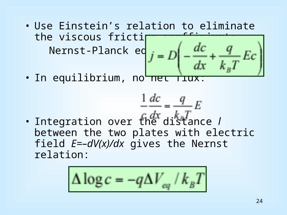
• Use Einstein’s relation to eliminate the viscous

friction-coefficient: Nernst-Planck equation:

• In equilibrium, no net flux:

• Integration over the distance l between the two plates with electric field E=–dV(x)/dx gives the Nernst relation:

24

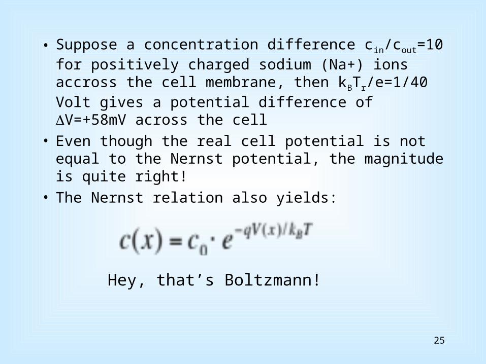
• Suppose a concentration difference cin/cout=10 for

positively charged sodium (Na+) ions accross the cell membrane, then kBTr/e=1/40 Volt gives a potential difference of V=+58mV across the cell

• Even though the real cell potential is not equal to the Nernst potential, the magnitude is quite right!

• The Nernst relation also yields:

Hey, that’s Boltzmann!

25

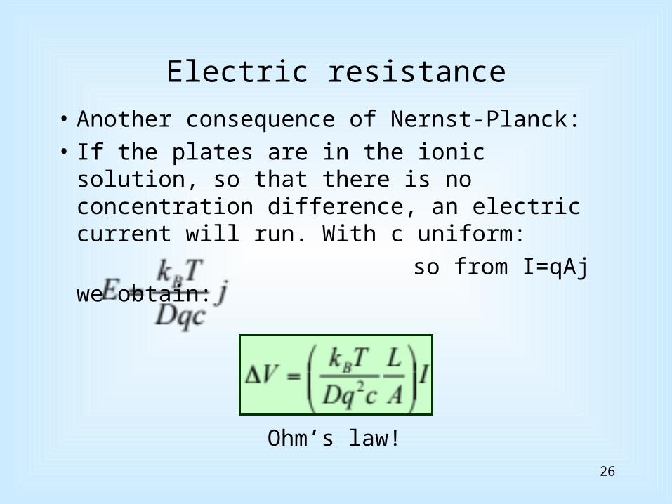
Electric resistance

• Another consequence of Nernst-Planck: • If the plates are in the ionic solution, so that

there is no concentration difference, an electric current will run. With c uniform:

so from I=qAj we obtain:

Ohm’s law!26

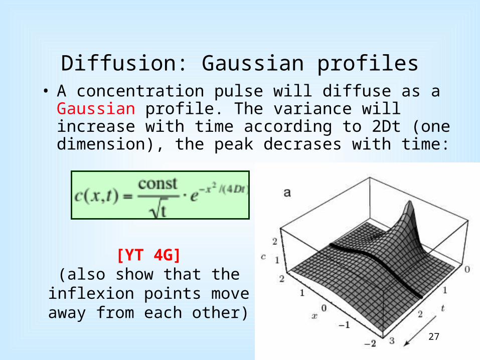
Diffusion: Gaussian profiles• A concentration pulse will diffuse as a Gaussian

profile. The variance will increase with time according to 2Dt (one dimension), the peak decrases with time:

[YT 4G](also show that the

inflexion points moveaway from each other)

27

Assignments:

• Your Turn 4G (show also that the inflextion points move away from each other)

• Exercises: 4.2, 4.4, 4.5 and 4.8 (< Nov 23)

• PLUS: Computer exercise (counts triple, and you get more time: < Xmas)

28