Embed Size (px)
Citation preview

Chapter 4 Network Layer
Computer Networking: A Top Down Approach 6th edition Jim Kurose, Keith Ross Addison-Wesley March 2012
Network Layer 4-1
Reti degli Elaboratori Canale AL Prof.ssa Chiara Petrioli a.a. 2013/2014 We thank for the support material Prof. Kurose-Ross All material copyright 1996-2012 J.F Kurose and K.W. Ross, All Rights Reserved
Network Layer 4-2
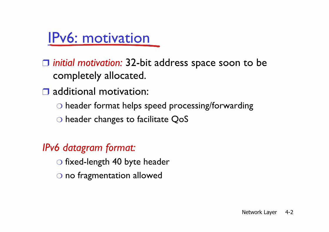
IPv6: motivation ❒ initial motivation: 32-bit address space soon to be
completely allocated. ❒ additional motivation:
❍ header format helps speed processing/forwarding ❍ header changes to facilitate QoS
IPv6 datagram format: ❍ fixed-length 40 byte header ❍ no fragmentation allowed

Network Layer 4-3
IPv6 datagram format
priority: identify priority among datagrams in flow flow Label: identify datagrams in same “flow.” (concept of“flow” not well defined). next header: identify upper layer protocol for data
data
destination address (128 bits)
source address (128 bits)
payload len next hdr hop limit flow label pri ver
32 bits

Network Layer 4-4
Other changes from IPv4
❒ checksum: removed entirely to reduce processing time at each hop
❒ options: allowed, but outside of header, indicated by “Next Header” field
❒ ICMPv6: new version of ICMP ❍ additional message types, e.g. “Packet Too Big” ❍ multicast group management functions

Network Layer 4-5
Transition from IPv4 to IPv6
❒ not all routers can be upgraded simultaneously ❍ no “flag days” ❍ how will network operate with mixed IPv4 and
IPv6 routers? ❒ tunneling: IPv6 datagram carried as payload in IPv4
datagram among IPv4 routers
IPv4 source, dest addr IPv4 header fields
IPv4 datagram IPv6 datagram
IPv4 payload
UDP/TCP payload IPv6 source dest addr
IPv6 header fields

Network Layer 4-6
Tunneling
physical view: IPv4 IPv4
A B
IPv6 IPv6
E
IPv6 IPv6
F C D
logical view:
IPv4 tunnel connecting IPv6 routers E
IPv6 IPv6
F A B
IPv6 IPv6

Network Layer 4-7
flow: X src: A dest: F data
A-to-B: IPv6
Flow: X Src: A Dest: F data
src:B dest: E
B-to-C: IPv6 inside
IPv4
E-to-F: IPv6
flow: X src: A dest: F data
B-to-C: IPv6 inside
IPv4
Flow: X Src: A Dest: F data
src:B dest: E
physical view: A B
IPv6 IPv6
E
IPv6 IPv6
F C D
logical view:
IPv4 tunnel connecting IPv6 routers E
IPv6 IPv6
F A B
IPv6 IPv6
Tunneling
IPv4 IPv4

Network Layer 4-8
Chapter 4: Network Layer
❒ 4. 1 Introduction ❒ 4.2 Virtual circuit and
datagram networks ❒ 4.3 What’s inside a
router ❒ 4.4 IP: Internet
Protocol ❍ Datagram format ❍ IPv4 addressing ❍ ICMP ❍ IPv6
❒ 4.5 Routing algorithms ❍ Link state ❍ Distance Vector ❍ Hierarchical routing
❒ 4.6 Routing in the Internet ❍ RIP ❍ OSPF ❍ BGP
❒ 4.7 Broadcast and multicast routing

Network Layer 4-9
1
2 3
0111
value in arriving packet’s header
routing algorithm
local forwarding table header value output link
0100 0101 0111 1001
3 2 2 1
Interplay between routing, forwarding

Network Layer 4-10
u
y x
w v
z 2
2 1 3
1
1 2
5 3
5
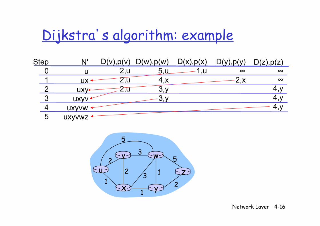
Graph: G = (N,E) N = set of routers = { u, v, w, x, y, z } E = set of links ={ (u,v), (u,x), (v,x), (v,w), (x,w), (x,y), (w,y), (w,z), (y,z) }
Graph abstraction
Remark: Graph abstraction is useful in other network contexts Example: P2P, where N is set of peers and E is set of TCP connections

Network Layer 4-11
Graph abstraction: costs
u
y x
w v
z 2
2 1 3
1
1 2
5 3
5 • c(x,x’) = cost of link (x,x’) - e.g., c(w,z) = 5 • cost could always be 1, or inversely related to bandwidth, or inversely related to congestion
Cost of path (x1, x2, x3,…, xp) = c(x1,x2) + c(x2,x3) + … + c(xp-1,xp)
Question: What’s the least-cost path between u and z ?
Routing algorithm: algorithm that finds least-cost path
Network Layer 4-12
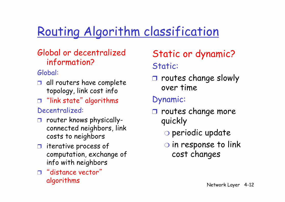
Routing Algorithm classification Global or decentralized
information? Global: ❒ all routers have complete
topology, link cost info ❒ “link state” algorithms Decentralized: ❒ router knows physically-
connected neighbors, link costs to neighbors
❒ iterative process of computation, exchange of info with neighbors
❒ “distance vector” algorithms
Static or dynamic? Static: ❒ routes change slowly
over time Dynamic: ❒ routes change more
quickly ❍ periodic update ❍ in response to link
cost changes
Network Layer 4-13
Chapter 4: Network Layer
❒ 4. 1 Introduction ❒ 4.2 Virtual circuit and
datagram networks ❒ 4.3 What’s inside a
router ❒ 4.4 IP: Internet
Protocol ❍ Datagram format ❍ IPv4 addressing ❍ ICMP ❍ IPv6
❒ 4.5 Routing algorithms ❍ Link state ❍ Distance Vector ❍ Hierarchical routing
❒ 4.6 Routing in the Internet ❍ RIP ❍ OSPF ❍ BGP
❒ 4.7 Broadcast and multicast routing
Network Layer 4-14
A Link-State Routing Algorithm
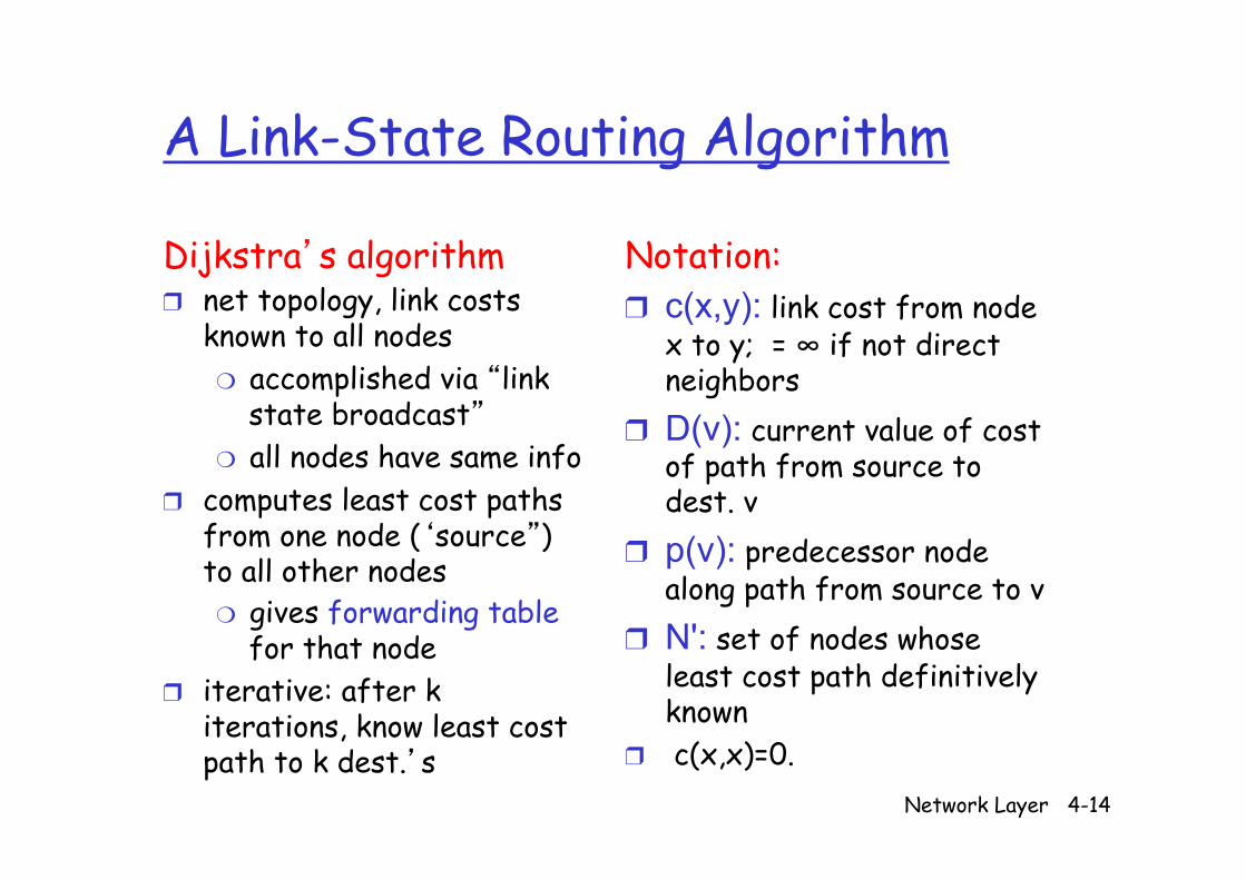
Dijkstra’s algorithm ❒ net topology, link costs
known to all nodes ❍ accomplished via “link
state broadcast” ❍ all nodes have same info
❒ computes least cost paths from one node (‘source”) to all other nodes ❍ gives forwarding table
for that node ❒ iterative: after k
iterations, know least cost path to k dest.’s
Notation: ❒ c(x,y): link cost from node
x to y; = ∞ if not direct neighbors
❒ D(v): current value of cost of path from source to dest. v
❒ p(v): predecessor node along path from source to v
❒ N': set of nodes whose least cost path definitively known
❒ c(x,x)=0.

Network Layer 4-15
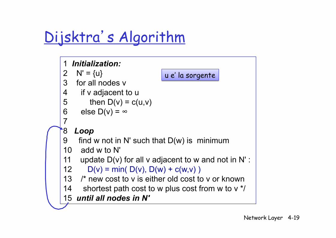
Dijsktra’s Algorithm 1 Initialization: 2 N' = {u} 3 for all nodes v 4 if v adjacent to u 5 then D(v) = c(u,v) 6 else D(v) = ∞ 7 8 Loop 9 find w not in N' such that D(w) is minimum 10 add w to N' 11 update D(v) for all v adjacent to w and not in N' : 12 D(v) = min( D(v), D(w) + c(w,v) ) 13 /* new cost to v is either old cost to v or known 14 shortest path cost to w plus cost from w to v */ 15 until all nodes in N'
u e’ la sorgente
Network Layer 4-16
Dijkstra’s algorithm: example Step
0 1 2 3 4 5
N' u
ux uxy
uxyv uxyvw
uxyvwz
D(v),p(v) 2,u 2,u 2,u
D(w),p(w) 5,u 4,x 3,y 3,y
D(x),p(x) 1,u
D(y),p(y) ∞
2,x
D(z),p(z) ∞ ∞
4,y 4,y 4,y
u
y x
w v
z 2
2 1 3
1
1 2
5 3
5

Network Layer 4-17
Dijkstra’s algorithm: example (2)
u
y x
w v
z
Resulting shortest-path tree from u:
v x y w z
(u,v) (u,x) (u,x) (u,x) (u,x)
destination link
Resulting forwarding table in u:

Dijkstra Algorithm-correctness
Network Layer 4-18
Teorema Se l’algoritmo di Dijkstra è eseguito su un grafo
G=(N,E) diretto e pesato i cui pesi sugli archi sono tutti non negativi, e con una sorgente s, allora Dijkstra termina con tutti i vertici w in N con valore D(w) pari alla lunghezza del cammino minimo da s a w.
Approccio: - Terminazione banale (perchè?) - Mostriamo che ogni volta che un vertice w è inserito in N’ allora
D(w) è pari alla lunghezza del cammino minimo da s a w
(dato che il valore di D(w) non viene ad essere mai più modificato dopo che w è inserito in N’-v. linea 11 dell’algoritmo- questo consente di dimostrare l’assunto).
Network Layer 4-19
Dijsktra’s Algorithm 1 Initialization: 2 N' = {u} 3 for all nodes v 4 if v adjacent to u 5 then D(v) = c(u,v) 6 else D(v) = ∞ 7 8 Loop 9 find w not in N' such that D(w) is minimum 10 add w to N' 11 update D(v) for all v adjacent to w and not in N' : 12 D(v) = min( D(v), D(w) + c(w,v) ) 13 /* new cost to v is either old cost to v or known 14 shortest path cost to w plus cost from w to v */ 15 until all nodes in N'
u e’ la sorgente

Dijkstra Algorithm-correctness
Network Layer 4-20
Mostriamo che ogni volta che un vertice w è inserito in N’ allora D(w) è pari alla lunghezza del cammino minimo da s a w
Si dimostra per assurdo. Sia u il primo nodo inserito in N’ che non rispetta la condizione, ovvero sia u il primo nodo che al momento del suo inserimento in N’ abbia D(u)!=δ(s,u), dove δ(s,u) denota la lunghezza del percorso minimo da s a u. u!=s dato che s è il primo nodo inserito in N’ e D(s)=δ(s,s)=0. Ci deve essere un percorso da s a u in G (altrimenti D(u)=infinity, e D(u)=δ(s,u)) e quindi anche un cammino minimo p da s a u. Prima di aggiungere u a N’ p univa un vertice in N’ ( il vertice s) and un vertice in N-N’ (il vertice u). Sia y il primo vertice in p non in N’, e x il suo predecessore.
s x y u p1 p2
Dijkstra Algorithm-correctness
Network Layer 4-21
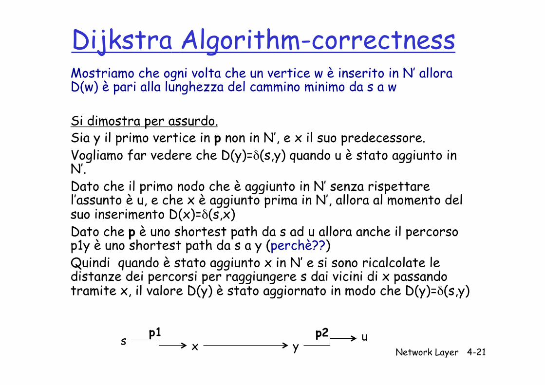
Mostriamo che ogni volta che un vertice w è inserito in N’ allora D(w) è pari alla lunghezza del cammino minimo da s a w
Si dimostra per assurdo. Sia y il primo vertice in p non in N’, e x il suo predecessore. Vogliamo far vedere che D(y)=δ(s,y) quando u è stato aggiunto in N’. Dato che il primo nodo che è aggiunto in N’ senza rispettare l’assunto è u, e che x è aggiunto prima in N’, allora al momento del suo inserimento D(x)=δ(s,x) Dato che p è uno shortest path da s ad u allora anche il percorso p1y è uno shortest path da s a y (perchè??) Quindi quando è stato aggiunto x in N’ e si sono ricalcolate le distanze dei percorsi per raggiungere s dai vicini di x passando tramite x, il valore D(y) è stato aggiornato in modo che D(y)=δ(s,y)
s x y u p1 p2

Dijkstra Algorithm-correctness
Network Layer 4-22
Mostriamo che ogni volta che un vertice w è inserito in N’ allora D(w) è pari alla lunghezza del cammino minimo da s a w
Si dimostra per assurdo. Vogliamo ora dimostrare che D(u)=δ(s,u) Dato che y viene prima di u in un percorso da s a u e tutti gli archi hanno pesi non negativi vale che δ(s,y)<=δ(s,u) e quindi D(y)=δ(s,y) <=δ(s,u) <=D(u) D’altra parte dato che sia u che y erano in N-N’ quando u è stato scelto per essere inserito in N’, al momento del suo inserimento D(u)<=D(y) (per la regola di selezione del vertice da inserire in N’) Quindi: D(y)=δ(s,y)=δ(s,u)=D(u) ASSURDO C.V.D s x y
u p1 p2

Network Layer 4-23
Dijsktra’s Algorithm 1 Initialization: 2 N' = {u} 3 for all nodes v 4 if v adjacent to u 5 then D(v) = c(u,v) 6 else D(v) = ∞ 7 8 Loop 9 find w not in N' such that D(w) is minimum 10 add w to N' 11 update D(v) for all v adjacent to w and not in N' : 12 D(v) = min( D(v), D(w) + c(w,v) ) 13 /* new cost to v is either old cost to v or known 14 shortest path cost to w plus cost from w to v */ 15 until all nodes in N'
u e’ la sorgente

Network Layer 4-24
Dijkstra’s algorithm, discussion Algorithm complexity: n nodes ❒ each iteration: need to check all nodes, w, not in N ❒ n(n+1)/2 comparisons: O(n2) ❒ more efficient implementations possible: O(nlogn+|E|) Oscillations possible: ❒ e.g., link cost = amount of carried traffic
A D
C B
1 1+e
e 0
e 1 1
0 0 A
D C
B 2+e 0
0 0 1+e 1
A D
C B
0 2+e
1+e 1 0 0
A D
C B
2+e 0
e 0 1+e 1
initially … recompute routing
… recompute … recompute

Network Layer 4-25
4.1 introduction 4.2 virtual circuit and
datagram networks 4.3 what’s inside a router 4.4 IP: Internet Protocol
❍ datagram format ❍ IPv4 addressing ❍ ICMP ❍ IPv6
4.5 routing algorithms ❍ link state ❍ distance vector ❍ hierarchical routing
4.6 routing in the Internet ❍ RIP ❍ OSPF ❍ BGP
4.7 broadcast and multicast routing
Chapter 4: outline

Network Layer 4-26
Bellman-Ford Given a graph G=(N,E) and a node s finds the shortest path
from s to every node in N. A shortest walk from s to i subject to the constraint that the walk
contains at most h arcs and goes through node s only once, is denoted shortest(<=h) walk and its length is Dh
i. Bellman-Ford rule: Initiatilization Dh
s=0, for all h; ci,k = infinity if (i,k) NOT in E; ck,k =0; D0
i=infinity for all i!=s. Iteration:
Dh+1i=mink [ci,k + Dh
k] Assumption: non negative cycles (this is the case in a network!!) The Bellman-Ford algorithm first finds the one-arc
shortest walk lengths, then the two-arc shortest walk length, then the three-arc…etc. àdistributed version used for routing

Network Layer 4-27
Bellman-Ford
Dh+1i=mink [ci,k + Dh
k]
Can be computed locally. What do I need? For each neighbor k, I need to know - the cost of the link to it (known info) - The cost of the best route from the neighbor k to the destination (this is an info that each of my neighbor has to send to me via messages) In the real world: I need to know the best routes among each pair of nodes we apply distributed Bellman Ford to get the best route for each of the possible destinations

Network Layer 4-28
Distance Vector Routing Algorithm -Distributed Bellman Ford
iterative: ❒ continues until no
nodes exchange info. ❒ self-terminating: no
“signal” to stop asynchronous: ❒ nodes need not
exchange info/iterate in lock step!
Distributed, based on local info:
❒ each node communicates only with directly-attached neighbors
Distance Table data structure each node has its own ❒ row for each possible destination ❒ column for each directly-
attached neighbor to node ❒ example: in node X, for dest. Y
via neighbor V: what is the cost?

Network Layer 4-29
Distance vector algorithm
Bellman-Ford equation (dynamic programming) let dx(y) := cost of least-cost path from x to y then
dx(y) = min {c(x,v) + dv(y) }
v
cost to neighbor v
min taken over all neighbors v of x
cost from neighbor v to destination y
Info maintained at v. Min must be communicated

Network Layer 4-30
Bellman-Ford example
u
y x
w v
z 2
2 1 3
1
1 2
5 3
5 clearly, dv(z) = 5, dx(z) = 3, dw(z) = 3
du(z) = min { c(u,v) + dv(z), c(u,x) + dx(z), c(u,w) + dw(z) } = min {2 + 5, 1 + 3, 5 + 3} = 4
node achieving minimum is next hop in shortest path, used in forwarding table
B-F equation says:

Network Layer 4-31
Distance vector algorithm
❒ Dx(y) = estimate of least cost from x to y ❍ x maintains distance vector Dx = [Dx(y): y є N ]
❒ node x: ❍ knows cost to each neighbor v: c(x,v) ❍ maintains its neighbors’ distance vectors. For
each neighbor v, x maintains Dv = [Dv(y): y є N ]

Network Layer 4-32
key idea: ❒ from time-to-time, each node sends its own
distance vector estimate to neighbors ❒ when x receives new DV estimate from neighbor,
it updates its own DV using B-F equation: Dx(y) ← minv{c(x,v) + Dv(y)} for each node y ∊ N
v under minor, natural conditions, the estimate Dx(y) converge to the actual least cost dx(y)
Distance vector algorithm

Network Layer 4-33
iterative, asynchronous: each local iteration caused by:
❒ local link cost change ❒ DV update message from
neighbor
distributed: ❒ each node notifies
neighbors only when its DV changes ❍ neighbors then notify their
neighbors if necessary
wait for (change in local link cost or msg from neighbor)
recompute estimates
if DV to any dest has changed, notify neighbors
each node:
Distance vector algorithm

Network Layer 4-34

Network Layer 4-35
x y z
x y z
0 2 7
∞ ∞ ∞ ∞ ∞ ∞
from
cost to fro
m
from
x y z
x y z
0
x y z
x y z
∞ ∞
∞ ∞ ∞
cost to
x y z
x y z ∞ ∞ ∞ 7 1 0
cost to
∞ 2 0 1
∞ ∞ ∞
2 0 1 7 1 0
time
x z 1 2
7
y
node x table
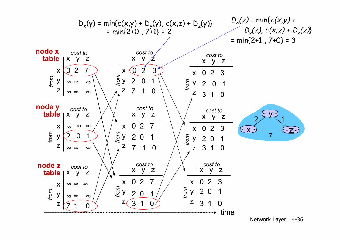
Dx(y) = min{c(x,y) + Dy(y), c(x,z) + Dz(y)} = min{2+0 , 7+1} = 2
Dx(z) = min{c(x,y) + Dy(z), c(x,z) + Dz(z)} = min{2+1 , 7+0} = 3
3 2
node y table
node z table
cost to fro
m
Network Layer 4-36
x y z
x y z
0 2 3
from
cost to
x y z
x y z
0 2 7 fro
m
cost to x y z
x y z
0 2 3
from
cost to
x y z
x y z
0 2 3 fro
m
cost to x y z
x y z
0 2 7
from
cost to
2 0 1 7 1 0
2 0 1 3 1 0
2 0 1 3 1 0
2 0 1
3 1 0
2 0 1
3 1 0
time
x y z
x y z
0 2 7
∞ ∞ ∞ ∞ ∞ ∞
from
cost to fro
m
from
x y z
x y z
0
x y z
x y z
∞ ∞
∞ ∞ ∞
cost to
x y z
x y z ∞ ∞ ∞ 7 1 0
cost to
∞ 2 0 1
∞ ∞ ∞
2 0 1 7 1 0
time
x z 1 2
7
y
node x table
Dx(y) = min{c(x,y) + Dy(y), c(x,z) + Dz(y)} = min{2+0 , 7+1} = 2
Dx(z) = min{c(x,y) + Dy(z), c(x,z) + Dz(z)} = min{2+1 , 7+0} = 3
3 2
node y table
node z table
cost to fro
m
Network Layer 4-37
Distance vector: link cost changes
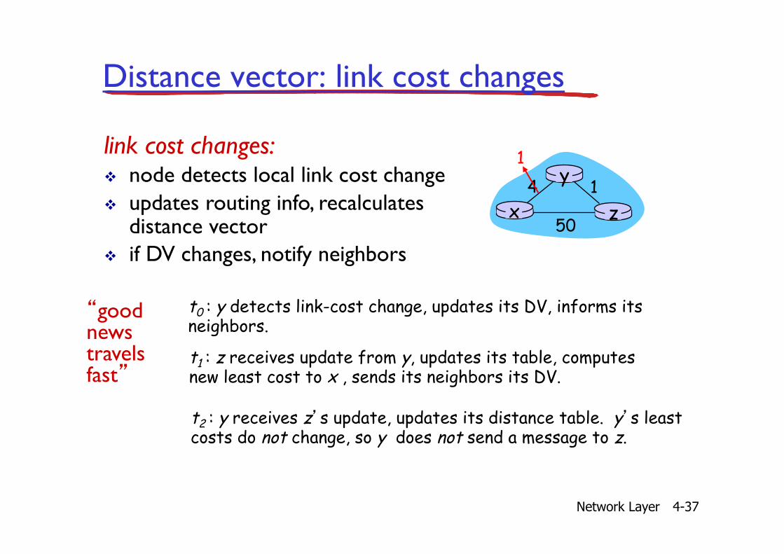
link cost changes: v node detects local link cost change v updates routing info, recalculates
distance vector v if DV changes, notify neighbors
“good news travels fast”
x z 1 4
50
y 1
t0 : y detects link-cost change, updates its DV, informs its neighbors. t1 : z receives update from y, updates its table, computes new least cost to x , sends its neighbors its DV. t2 : y receives z’s update, updates its distance table. y’s least costs do not change, so y does not send a message to z.

Network Layer 4-38
Distance vector: link cost changes
link cost changes: v node detects local link cost change v bad news travels slow - “count to
infinity” problem! v 44 iterations before algorithm
stabilizes: see text
x z 1 4
50
y 60
poisoned reverse: v If Z routes through Y to get to X :
§ Z tells Y its (Z’s) distance to X is infinite (so Y won’t route to X via Z)
v will this completely solve count to infinity problem?

39
Distributed Bellman Ford-Count to Infinity (we will now use a slightly different notation- lightweigh)
Distance Table data structure each node has its own ❒ row for each possible destination ❒ column for each directly-attached
neighbor to node ❒ example: in node X, for dest. Y via
neighbor Z:
D (Y,Z) X
distance from X to Y, via Z as next hop
c(X,Z) + min {D (Y,w)} Z w
=
=
Cost associated to the (X,Z) link
Info maintained at Z. Min must be communicated

40
Distance Vector: link cost changes
Link cost changes: • good news travels fast • bad news travels slow - “count to
infinity” problem! X Z
1 4
50
Y 60
algorithm continues
on!
Y detects link cost Increase but think can Reach X through Z at a total cost of 6 (wrong!!)
The path is Y-Z-Y-X

41
Count-to-infinity – an everyday life example
Which is the problem here? the info exchanged by the protocol!! ‘the best route to X I have has the following cost…’ (no additional info on the route) A Roman example… -assumption: there is only one route going from Colosseo to Altare della Patria: Via dei Fori Imperiali. Let us now consider a network, whose nodes are Colosseo., Altare della Patria, Piazza del Popolo
Colosseo Altare Patria Piazza del Popolo
1 Km 1 Km

42
Colosseo Al.Patria P.Popolo 1Km 1Km
The Colosseo. and Alt. Patria nodes exchange the following info • Colosseo says ‘the shortest route from me to P. Popolo is 2 Km’ • Alt. Patria says ‘the shortest path from me to P. Popolo is 1Km’ Based on this exchange from Colosseo you go to Al. Patria, and from there to Piazza del Popolo OK Now due to the big dig they close Via del Corso (Al. Patria—P.Popolo) • Al. Patria thinks ‘I have to find another route from me to P.Popolo. Look there is a route from Colosseo to P.Popolo that takes 2Km, I can be at Colosseo in 1Km à I have found a 3Km route from me to P.Popolo!!’ Communicates the new cost to Colosseo that updates ‘OK I can go to P.Popolo via Al. Patria in 4Km’ VERY WRONG!! Why is it so? I didn’t know that the route from Colosseo to P.Popolo was going through Via del Corso from Al.Patria to P.Popolo (which is closed)!!
Count-to-infinity – everyday life example (2/2)

Network Layer 4-43
Distance vector: link cost changes
link cost changes: v node detects local link cost change v bad news travels slow - “count to
infinity” problem! v 44 iterations before algorithm
stabilizes: see text
x z 1 4
50
y 60
poisoned reverse: v If Z routes through Y to get to X :
§ Z tells Y its (Z’s) distance to X is infinite (so Y won’t route to X via Z)
v will this completely solve count to infinity problem?
Network Layer 4-44
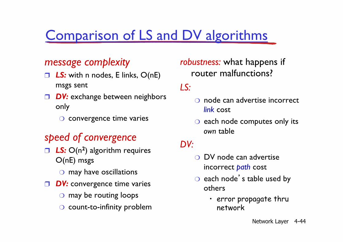
Comparison of LS and DV algorithms
message complexity ❒ LS: with n nodes, E links, O(nE)
msgs sent ❒ DV: exchange between neighbors
only ❍ convergence time varies
speed of convergence ❒ LS: O(n2) algorithm requires
O(nE) msgs ❍ may have oscillations
❒ DV: convergence time varies ❍ may be routing loops ❍ count-to-infinity problem
robustness: what happens if router malfunctions?
LS: ❍ node can advertise incorrect
link cost ❍ each node computes only its
own table
DV: ❍ DV node can advertise
incorrect path cost ❍ each node’s table used by
others • error propagate thru
network