Chapter 4. The response of the climate system to a ... · PDF fileThe response of the climate system to a perturbation . 4.1 Climate forcing and ... The response of the climate system

Introduction to climate dynamics and climate modelling - http://www.climate.be/textbook

Chapter 4. The response of the climate system to a perturbation

4.1 Climate forcing and climate response 4.1.1 Notion of radiative forcing The climate system is influenced by different types of perturbation: changes in the

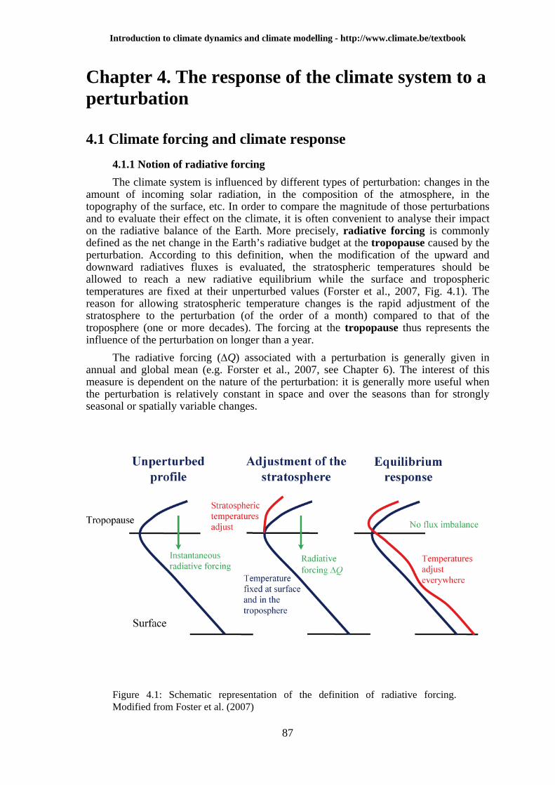
amount of incoming solar radiation, in the composition of the atmosphere, in the topography of the surface, etc. In order to compare the magnitude of those perturbations and to evaluate their effect on the climate, it is often convenient to analyse their impact on the radiative balance of the Earth. More precisely, radiative forcing is commonly defined as the net change in the Earth’s radiative budget at the tropopause caused by the perturbation. According to this definition, when the modification of the upward and downward radiatives fluxes is evaluated, the stratospheric temperatures should be allowed to reach a new radiative equilibrium while the surface and tropospheric temperatures are fixed at their unperturbed values (Forster et al., 2007, Fig. 4.1). The reason for allowing stratospheric temperature changes is the rapid adjustment of the stratosphere to the perturbation (of the order of a month) compared to that of the troposphere (one or more decades). The forcing at the tropopause thus represents the influence of the perturbation on longer than a year.

The radiative forcing (ΔQ) associated with a perturbation is generally given in annual and global mean (e.g. Forster et al., 2007, see Chapter 6). The interest of this measure is dependent on the nature of the perturbation: it is generally more useful when the perturbation is relatively constant in space and over the seasons than for strongly seasonal or spatially variable changes.

Figure 4.1: Schematic representation of the definition of radiative forcing. Modified from Foster et al. (2007)

87

Goosse H., P.Y. Barriat, W. Lefebvre, M.F. Loutre and V. Zunz (2010)

4.1.2 Major radiative forcings 4.1.2.1 Greenhouse gases The main radiative forcings that have affected the Earth’s climate can be grouped

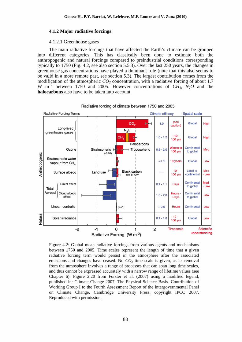
into different categories. This has classically been done to estimate both the anthropogenic and natural forcings compared to preindustrial conditions corresponding typically to 1750 (Fig. 4.2, see also section 5.5.3). Over the last 250 years, the changes in greenhouse gas concentrations have played a dominant role (note that this also seems to be valid in a more remote past, see section 5.3). The largest contribution comes from the modification of the atmospheric CO2 concentration, with a radiative forcing of about 1.7 W m–2 between 1750 and 2005. However concentrations of CH4, N2O and the halocarbons also have to be taken into account.

Figure 4.2: Global mean radiative forcings from various agents and mechanisms between 1750 and 2005. Time scales represent the length of time that a given radiative forcing term would persist in the atmosphere after the associated emissions and changes have ceased. No CO2 time scale is given, as its removal from the atmosphere involves a range of processes that can span long time scales, and thus cannot be expressed accurately with a narrow range of lifetime values (see Chapter 6). Figure 2.20 from Forster et al. (2007) using a modified legend, published in: Climate Change 2007: The Physical Science Basis. Contribution of Working Group I to the Fourth Assessment Report of the Intergovernmental Panel on Climate Change, Cambridge University Press, copyright IPCC 2007. Reproduced with permission.

88

4. The response of the climate system to a perturbation

Estimating the radiative forcing ΔQ associated with the changes in the concentrations of these gases requires a comprehensive radiative transfer model. However, relatively good approximations can be obtained for CO2 from a simple formula:

[ ][ ]

2

2

5.4lnr

COQ

CO⎛ ⎞

Δ = ⎜⎜⎝ ⎠

⎟⎟ (4.1)

where [CO2] and [CO2]r are the CO2 concentrations in ppm for the period being investigated and for a reference period, respectively. Similar approximations can be made for CH4 and N2O:

[ ] [ ]( )Δ = −4 40.036r

Q CH CH (4.2)

[ ]( )2 20.12 rQ N O NΔ = − O (4.3)

where the same notation is used as in Eq. 4.1, the concentrations being in ppb. For halocarbons, a linear expression appears valid. When evaluating the radiative

forcing since 1750, reference values for this period are classically: CO2 (278ppm), CH4 (715 ppb), N2O (270 ppb) (see in Forster et al 2007).

CO2, CH4, N2O and halocarbons are long-lived gases that remain in the atmosphere for decades if not centuries. Their geographical distribution is thus quite homogenous, with only small differences between the two hemispheres. Other greenhouse gases such as O3 (ozone) have a shorter life. As a consequence, their concentration, and thus the associated radiative forcing, tend to be higher close to areas where there are produced, and lower near areas where they are destroyed. Tropospheric ozone is mainly formed through photochemical reactions driven by the emission of various nitrous oxides, carbon monoxide and some volatile organic compounds. Globally, the impact of the increase in its concentration is estimated to induce a radiative forcing around 0.35 W m–2. However, the forcing is higher close to industrial regions, where the gases leading to ozone production are released. By contrast, stratospheric ozone has decreased since pre-industrial time, leading to a globally average radiative forcing of –0.05 W m–2. The stratospheric ozone changes are particularly large in polar regions, as the reactions responsible for the destruction of ozone in the presence of some chemical compounds (such as chlorofluorocarbons) are more efficient at low temperatures. The largest decrease is observed over the high latitudes of the Southern Hemisphere. There, the famous ozone hole, discovered in the mid 1980’s, is a large region of the stratosphere where about half the ozone disappears in spring. Because of the Montreal Protocol which bans the use of chlorofluorocarbons, the concentration of these gases in the atmosphere is no longer increasing, and may even be decreasing slowly. However ozone recovery in the stratosphere is not yet clear.

4.1.2.2 Aerosols Atmospheric aerosols are relatively small solid or liquid particles that are

suspended in the atmosphere. They are largely natural: they may be generated by evaporation of sea spray, by wind blowing over dusty regions, by forest and grassland fires, by living vegetation (such as the production of sulphur aerosols by phytoplankton), by volcanoes (see section 4.1.2.4), etc. Human activities also produce aerosols by burning

89


fossil fuels or biomass, and by the modification of natural surface cover that influences the amount of dust carried by the wind. Among the anthropogenic aerosols, those that have received the most attention in climatology are sulphate aerosols and black carbon. Sulphate is mainly produced by the oxidation of sulphur dioxide (SO2) in the aqueous phase, with fossil fuel burning, in particular coal burning, as their main source. Black carbon is the result of incomplete combustion during fossil fuel and biomass burning.

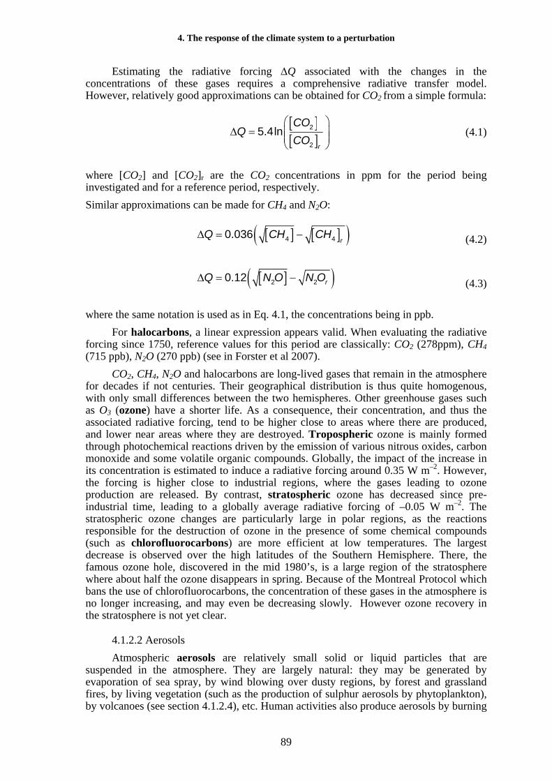
Since the majority of aerosols only remain in the atmosphere for a few days, anthropogenic aerosols are mainly concentrated downwind of industrial areas, close to regions where land-use changes have led to dustier surfaces (desertification) and where slash-and-burn agricultural practices are common. As a consequence, maximum concentrations are found in Eastern America, Europe, and Eastern Asia as well as in some regions of tropical Africa and South America (Fig. 4.3).

Figure 4.3: Aerosol optical depths (i.e. a measure of atmospheric transparency) for black carbon (BC, x10) (a) in 1890, (b) in 1995, and (c) the change between 1890 and 1995; (d)–(f) the same measures for sulphates (SO4). Reproduced from Koch et al. (2008). Copyright 2009 American Meteorological Society (AMS).

Aerosols affect directly our environment as they are responsible, for instance, for health problems and acid rain. They also have multiple direct, indirect and semi-direct effects on the radiative properties of the atmosphere (Fig. 4.4). The direct effects of aerosols are related to how they absorb and scatter shortwave and longwave radiation. For sulphate aerosols, the main effect is the net scattering of a significant fraction of the incoming solar radiation back to space (Fig. 4.4). This induces a negative radiative forcing, estimated to be around –0.4 W m–2 on average across the globe. This distribution is highly heterogeneous because of regional variations in the concentration of aerosols (see Fig. 4.3). By contrast, the main effect of black carbon is its strong absorption of solar radiation, which tends to warm the local air mass. The associated positive radiative forcing since 1750 is about +0.2 W m–2 on average. Furthermore, the deposit of black carbon on snow modifies snow’s albedo, generating an additional small positive forcing (~+0.1 W m–2). Taking all the aerosols (but not the effect of black carbon on albedo) into account, the global average of the total direct aerosol effect is about –0.50 W m–2 (Fig. 4.2).

90


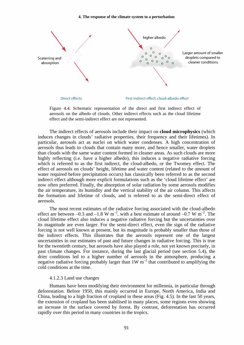
Figure 4.4: Schematic representation of the direct and first indirect effect of aerosols on the albedo of clouds. Other indirect effects such as the cloud lifetime effect and the semi-indirect effect are not represented.

The indirect effects of aerosols include their impact on cloud microphysics (which induces changes in clouds’ radiative properties, their frequency and their lifetimes). In particular, aerosols act as nuclei on which water condenses. A high concentration of aerosols thus leads to clouds that contain many more, and hence smaller, water droplets than clouds with the same water content formed in cleaner areas. As such clouds are more highly reflecting (i.e. have a higher albedo), this induces a negative radiative forcing which is referred to as the first indirect, the cloud-albedo, or the Twomey effect. The effect of aerosols on clouds’ height, lifetime and water content (related to the amount of water required before precipitation occurs) has classically been referred to as the second indirect effect although more explicit formulations such as the ‘cloud lifetime effect’ are now often preferred. Finally, the absorption of solar radiation by some aerosols modifies the air temperature, its humidity and the vertical stability of the air column. This affects the formation and lifetime of clouds, and is referred to as the semi-direct effect of aerosols.

The most recent estimates of the radiative forcing associated with the cloud-albedo effect are between –0.3 and –1.8 W m–2, with a best estimate of around –0.7 W m–2. The cloud lifetime effect also induces a negative radiative forcing but the uncertainties over its magnitude are even larger. For the semi-direct effect, even the sign of the radiative forcing is not well known at present, but its magnitude is probably smaller than those of the indirect effects. This illustrates that the aerosols represent one of the largest uncertainties in our estimates of past and future changes in radiative forcing. This is true for the twentieth century, but aerosols have also played a role, not yet known precisely, in past climate changes. For instance, during the last glacial period (see section 5.4), the drier conditions led to a higher number of aerosols in the atmosphere, producing a negative radiative forcing probably larger than 1W m–2 that contributed to amplifying the cold conditions at the time.

4.1.2.3 Land use changes Humans have been modifying their environment for millennia, in particular through

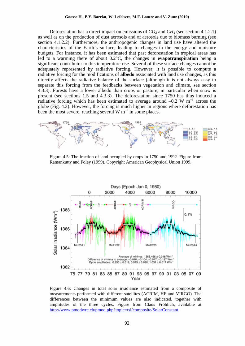
deforestation. Before 1950, this mainly occurred in Europe, North America, India and China, leading to a high fraction of cropland in these areas (Fig. 4.5). In the last 50 years, the extension of cropland has been stabilised in many places, some regions even showing an increase in the surface covered by forest. By contrast, deforestation has occurred rapidly over this period in many countries in the tropics.

91


Deforestation has a direct impact on emissions of CO2 and CH4 (see section 4.1.2.1) as well as on the production of dust aerosols and of aerosols due to biomass burning (see section 4.1.2.2). Furthermore, the anthropogenic changes in land use have altered the characteristics of the Earth’s surface, leading to changes in the energy and moisture budgets. For instance, it has been estimated that past deforestation in tropical areas has led to a warming there of about 0.2°C, the changes in evapotranspiration being a significant contributor to this temperature rise. Several of these surface changes cannot be adequately represented by radiative forcing. However, it is possible to compute a radiative forcing for the modifications of albedo associated with land use changes, as this directly affects the radiative balance of the surface (although it is not always easy to separate this forcing from the feedbacks between vegetation and climate, see section 4.3.3). Forests have a lower albedo than crops or pasture, in particular when snow is present (see sections 1.5 and 4.3.3). The deforestation since 1750 has thus induced a radiative forcing which has been estimated to average around –0.2 W m–2 across the globe (Fig. 4.2). However, the forcing is much higher in regions where deforestation has been the most severe, reaching several W m–2 in some places.

Figure 4.5: The fraction of land occupied by crops in 1750 and 1992. Figure from Ramankutty and Foley (1999). Copyright American Geophysical Union 1999.

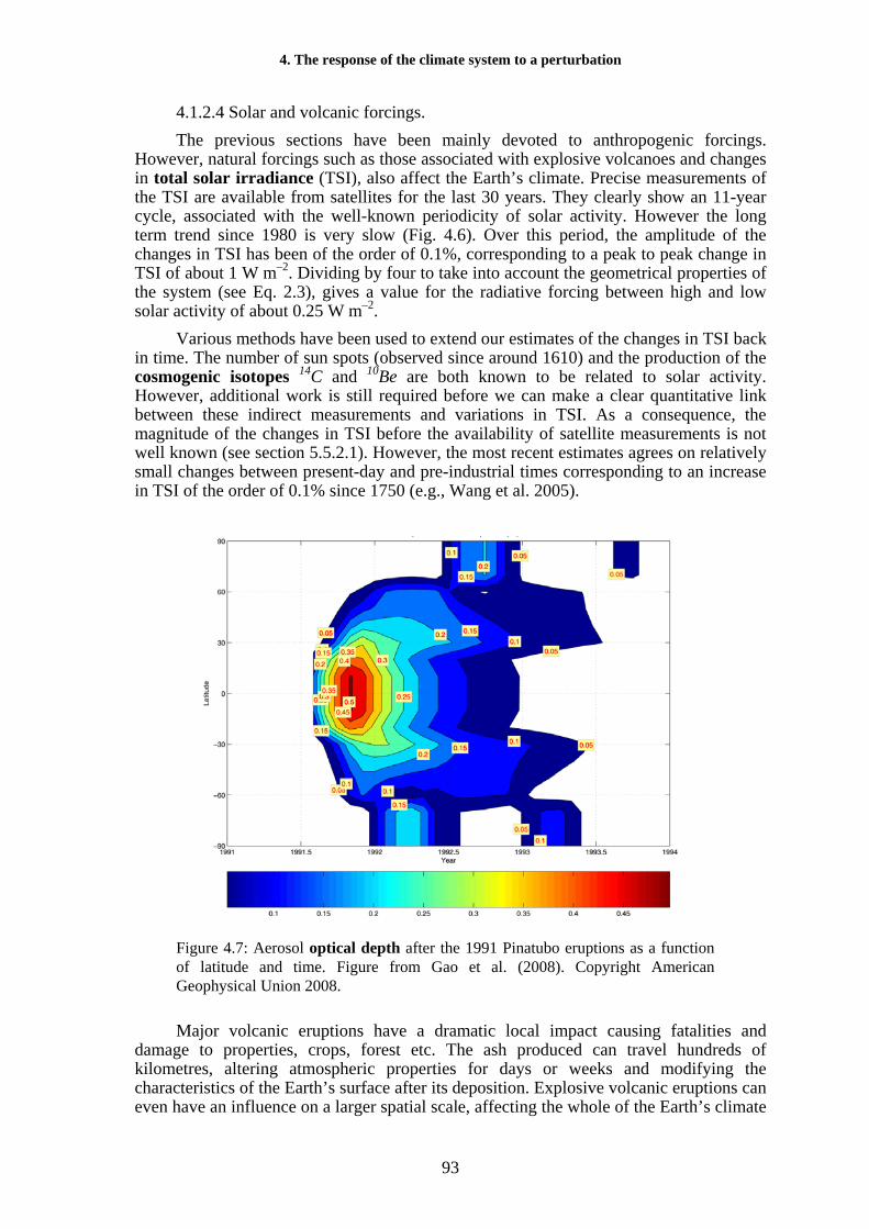
Figure 4.6: Changes in total solar irradiance estimated from a composite of measurements performed with different satellites (ACRIM, HF and VIRGO). The differences between the minimum values are also indicated, together with amplitudes of the three cycles. Figure from Claus Fröhlich, available at http://www.pmodwrc.ch/pmod.php?topic=tsi/composite/SolarConstant.

92

http://www.pmodwrc.ch/pmod.php?topic=tsi/composite/SolarConstant


4.1.2.4 Solar and volcanic forcings. The previous sections have been mainly devoted to anthropogenic forcings.

However, natural forcings such as those associated with explosive volcanoes and changes in total solar irradiance (TSI), also affect the Earth’s climate. Precise measurements of the TSI are available from satellites for the last 30 years. They clearly show an 11-year cycle, associated with the well-known periodicity of solar activity. However the long term trend since 1980 is very slow (Fig. 4.6). Over this period, the amplitude of the changes in TSI has been of the order of 0.1%, corresponding to a peak to peak change in TSI of about 1 W m–2. Dividing by four to take into account the geometrical properties of the system (see Eq. 2.3), gives a value for the radiative forcing between high and low solar activity of about 0.25 W m–2.

Various methods have been used to extend our estimates of the changes in TSI back in time. The number of sun spots (observed since around 1610) and the production of the cosmogenic isotopes 14C and 10Be are both known to be related to solar activity. However, additional work is still required before we can make a clear quantitative link between these indirect measurements and variations in TSI. As a consequence, the magnitude of the changes in TSI before the availability of satellite measurements is not well known (see section 5.5.2.1). However, the most recent estimates agrees on relatively small changes between present-day and pre-industrial times corresponding to an increase in TSI of the order of 0.1% since 1750 (e.g., Wang et al. 2005).

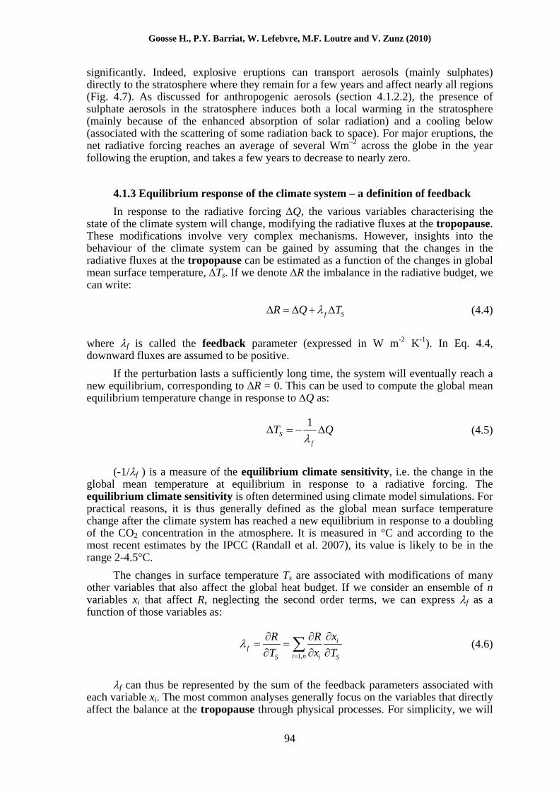
Figure 4.7: Aerosol optical depth after the 1991 Pinatubo eruptions as a function of latitude and time. Figure from Gao et al. (2008). Copyright American Geophysical Union 2008.

Major volcanic eruptions have a dramatic local impact causing fatalities and damage to properties, crops, forest etc. The ash produced can travel hundreds of kilometres, altering atmospheric properties for days or weeks and modifying the characteristics of the Earth’s surface after its deposition. Explosive volcanic eruptions can even have an influence on a larger spatial scale, affecting the whole of the Earth’s climate

93


significantly. Indeed, explosive eruptions can transport aerosols (mainly sulphates) directly to the stratosphere where they remain for a few years and affect nearly all regions (Fig. 4.7). As discussed for anthropogenic aerosols (section 4.1.2.2), the presence of sulphate aerosols in the stratosphere induces both a local warming in the stratosphere (mainly because of the enhanced absorption of solar radiation) and a cooling below (associated with the scattering of some radiation back to space). For major eruptions, the net radiative forcing reaches an average of several Wm–2 across the globe in the year following the eruption, and takes a few years to decrease to nearly zero.

4.1.3 Equilibrium response of the climate system – a definition of feedback In response to the radiative forcing ΔQ, the various variables characterising the

state of the climate system will change, modifying the radiative fluxes at the tropopause. These modifications involve very complex mechanisms. However, insights into the behaviour of the climate system can be gained by assuming that the changes in the radiative fluxes at the tropopause can be estimated as a function of the changes in global mean surface temperature, ΔTs. If we denote ΔR the imbalance in the radiative budget, we can write:

f SR Q TλΔ = Δ + Δ (4.4)

where λf is called the feedback parameter (expressed in W m-2 K-1). In Eq. 4.4, downward fluxes are assumed to be positive.

If the perturbation lasts a sufficiently long time, the system will eventually reach a new equilibrium, corresponding to ΔR = 0. This can be used to compute the global mean equilibrium temperature change in response to ΔQ as:

1S

f

Tλ

QΔ = − Δ (4.5)

(-1/λf ) is a measure of the equilibrium climate sensitivity, i.e. the change in the global mean temperature at equilibrium in response to a radiative forcing. The equilibrium climate sensitivity is often determined using climate model simulations. For practical reasons, it is thus generally defined as the global mean surface temperature change after the climate system has reached a new equilibrium in response to a doubling of the CO2 concentration in the atmosphere. It is measured in °C and according to the most recent estimates by the IPCC (Randall et al. 2007), its value is likely to be in the range 2-4.5°C.

The changes in surface temperature Ts are associated with modifications of many other variables that also affect the global heat budget. If we consider an ensemble of n variables xi that affect R, neglecting the second order terms, we can express λf as a function of those variables as:

1,

if

i nS i S

xR RT x

λ= T

∂∂ ∂= =

∂ ∂ ∂∑ (4.6)

λf can thus be represented by the sum of the feedback parameters associated with each variable xi. The most common analyses generally focus on the variables that directly affect the balance at the tropopause through physical processes. For simplicity, we will

94


call these the direct physical feedbacks (section 4.2). The standard decomposition of λf then involves their separation into feedbacks related to the temperature (λT), the water vapour (λw), the clouds (λc) and the surface albedo (λα). The temperature feedback is itself further split as λT = λ0 + λL. In evaluating λ0, we assume that the temperature changes are uniform throughout the troposphere, while λL, is called the lapse rate feedback (see section 4.2.1), and is the feedback due to the non-uniformity of temperature changes over the vertical. Thus

0f i L w ci

αλ λ λ λ λ λ λ= = + + + +∑ (4.7)

Although indirect effects (such as changes in ocean or atmospheric dynamics and biogeochemical feedbacks) can also play an important role, they are excluded from this decomposition. Biogeochemical feedbacks will be discussed in section 4.3. Some indirect feedbacks, in which the dominant processes cannot be simply related to the heat balance at the tropopause will be mentioned briefly in Chapters 5 and 6, but a detailed analysis is left for more advanced courses.

The feedback parameter λ0 can be evaluated relatively easily because it simply represents the dependence of the outgoing longwave radiation on temperature through the Stefan-Boltzmann law. Using the integrated balance at the top of the atmosphere (see section 2.1):

40(1 )4 eSR Tα σ= − − (4.8)

and assuming the temperature changes to be homogenous in the troposphere

S eT T TΔ = Δ = Δ (4.9)

we obtain

30 4 e

R T TT T

λ σ∂ ∂= = −

∂ ∂ (4.10)

This provides a value of λ0~-3.8 W m-2 K-1. More precise estimates using climate models gives a value of around −3.2 W m-2 K-1.

We can then compute the equilibrium temperature change in response to a perturbation if this feedback was the only one active as:

,00

SQT

λΔ

Δ = − (4.11)

For a radiative forcing due to a doubling of the CO2 concentration in the atmosphere corresponding to about 3.8 W m-2 (see Chapter 6), Eq. 4.11 leads to a climate sensitivity that would be slightly greater than 1°C.

95


If now, we include all the feedbacks, we can write:

0S

i L w ci

Q QTαλ λ λ λ λ λ

Δ ΔΔ = − = −

+ + + +∑ (4.12)

All these feedbacks are often compared to the blackbody response of the system, represented by λ0, of:

0

0 0 0 0

,0

0 0 0 0

,0

1

1

1

1

Sw cL

Sw cL

f S

QT

T

f T

α

α

λλ λ λλλ λ λ λ

λ λ λλλ λ λ λ

⎛ ⎞ΔΔ = − ⎜ ⎟⎛ ⎞ ⎝ ⎠+ + + +⎜ ⎟

⎝ ⎠

=⎛

+ + + +⎜ ⎟⎝ ⎠

= Δ

Δ⎞

(4.13)

Here ff is called the feedback factor. If ff is larger than one, it means that the equilibrium temperature response of the system is larger than the response of a blackbody. As λ0 is negative, Eq. 4.13 also shows that, if a feedback parameter λi is positive, the corresponding feedback amplifies the temperature changes (positive feedback). However, if λi is negative, it damps down the changes (negative feedback).

The concepts of radiative forcing, climate feedback and climate sensitivity are very useful in providing a general overview of the behaviour of the system. However, when using them, we must bear in mind that the framework described above is a greatly simplified version of a complex three-dimensional system. First, it does not provide explicit information on many important climate variables such as the spatial distribution of the changes or the probability of extreme events such as storms or hurricanes. Second, the magnitude of the climate feedbacks and the climate sensitivity depends on the forcing applied. Climate sensitivity is usually defined through the response of the system to a increase in CO2 concentration but some types of forcing are more ‘efficient’ than others for the same radiative forcing, meaning that they induce larger responses. Third, the feedbacks depend on the mean state of the climate system. For instance, it is pretty obvious that feedbacks related to the cryosphere (see section 4.3) play a larger role in relatively cold periods, where large amounts of ice are present at the surface, than in warmer periods. Fourth, non-linearities in the climate system lead to large modifications when a threshold is crossed as a response to the perturbation (see for instance section 4.3). In such cases, the climate change is mainly due to the internal dynamics of the system and is only weakly related to the magnitude of the forcing. Consequently, the assumptions leading to Eq. 4.4 are no longer valid.

4.1.4 Transient response of the climate system Because of the thermal inertia of the Earth (see section 2.1.5), the equilibrium

response described in section 4.1.2 is only achieved when all the components of the system have adjusted to the new forcing. It can take years or decades for the atmosphere, and centuries or millennia for the seas and the ice sheets, to reach this new equilibrium.

96


Following the same approach as in sections 4.1.1 and 4.1.2, we will assume that the thermal inertia can be represented at the first order by a slab with homogenous temperature Ts and heat capacity Cs. Using the same notation as for Eq. 4.4, the energy balance of the system can be written as:

Ss f S

d TC Qdt

λ TΔ= Δ + Δ (4.14)

If we assume that the radiative forcing ΔQ is equal to zero for t<0 and is constant for , this equation can easily be solved, leading to: 0t ≥

( /1 tS

f

QT )e τ

λ−Δ

Δ = − − (4.15)

with

s

f

Cτλ

= − (4.16)

When t is very large, we obtain, as expected, the equilibrium solution described by Eq. 4.5. τ represents a timescale, and when t= τ, the temperature change has reached 63% of its equilibrium value. τ is dependent on the heat capacity of the system Cs and on the strength of the feedbacks. This implies that with larger values of (-1/λf) (i.e. greater climate sensitivity) the time taken to reach equilibrium will be longer. This is an important characteristic of the climate system, which also holds when much more sophisticated representations of the climate system than the one shown in Eq. 4.14 are used.

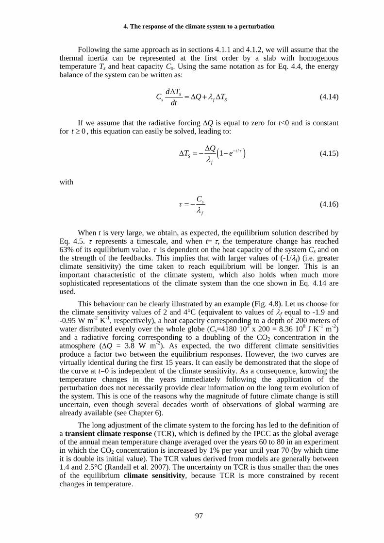
This behaviour can be clearly illustrated by an example (Fig. 4.8). Let us choose for the climate sensitivity values of 2 and 4°C (equivalent to values of λf equal to -1.9 and -0.95 W m-2 K-1, respectively), a heat capacity corresponding to a depth of 200 meters of water distributed evenly over the whole globe (Cs=4180 103 x 200 = 8.36 108 J K-1 m-2) and a radiative forcing corresponding to a doubling of the CO2 concentration in the atmosphere (ΔQ = 3.8 W m-2). As expected, the two different climate sensitivities produce a factor two between the equilibrium responses. However, the two curves are virtually identical during the first 15 years. It can easily be demonstrated that the slope of the curve at t=0 is independent of the climate sensitivity. As a consequence, knowing the temperature changes in the years immediately following the application of the perturbation does not necessarily provide clear information on the long term evolution of the system. This is one of the reasons why the magnitude of future climate change is still uncertain, even though several decades worth of observations of global warming are already available (see Chapter 6).

The long adjustment of the climate system to the forcing has led to the definition of a transient climate response (TCR), which is defined by the IPCC as the global average of the annual mean temperature change averaged over the years 60 to 80 in an experiment in which the CO2 concentration is increased by 1% per year until year 70 (by which time it is double its initial value). The TCR values derived from models are generally between 1.4 and 2.5°C (Randall et al. 2007). The uncertainty on TCR is thus smaller than the ones of the equilibrium climate sensitivity, because TCR is more constrained by recent changes in temperature.

97


Before closing this section, it is important to mention that some changes can be classified as either forcing or response depending on the particular focus of the investigator. For instance, in a study of glacial-interglacial climate changes, the building of ice sheets is generally considered as a response of the system to orbital forcing, implying powerful feedbacks (see Chapter 5). On the other hand, if an investigator is mainly interested in atmospheric and oceanic circulation during glacial periods, the ice sheets could be treated as boundary conditions and their influence on the Earth’s radiative balance (in particular through their albedo) as a radiative forcing. This distinction between forcing and response can, in some cases, be even more subtle. It is thus important in climatology, as in many other disciplines, to define precisely what we consider the system we are studying to be, and what are the boundary conditions and forcings.

Figure 4.8: Temperature changes obtained as a solution of Eq. 4.14, using a forcing ΔQ of 3.8 W m-2,Cs equal to 8.36 108 J K-1 m-2 and values of λf of -1.9 (black) and -0.95 W m-2 K-1 (red).

4.2 Direct physical feedbacks

4.2.1 Water vapour feedback and lapse rate feedback According to the Clausius-Clapeyron equation, the saturation vapour pressure

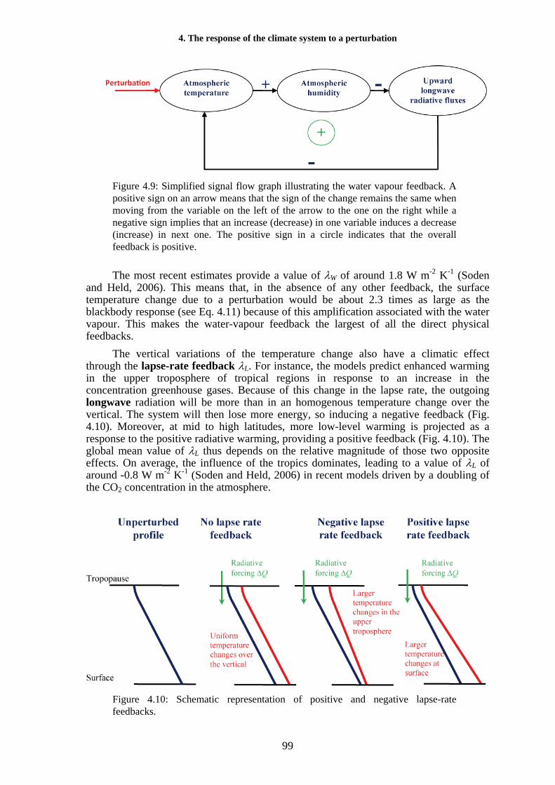
and the specific humidity at saturation are quasi-exponential functions of temperature. Furthermore, observations and numerical experiments consistently show that the relative humidity tends to remain more or less constant in response to climate change. A warming thus produces a significant increase in the amount of water vapour in the atmosphere. As water vapour is an efficient greenhouse gas, this leads to a strong positive feedback (Fig. 4.9). The radiative effect of water vapour is roughly proportional to the logarithm of its concentration, and so the influence of an increase in water-vapour content is larger in places where its concentration is relatively low in unperturbed conditions, such as in the upper troposphere (see section 1.2.1).

98


Figure 4.9: Simplified signal flow graph illustrating the water vapour feedback. A positive sign on an arrow means that the sign of the change remains the same when moving from the variable on the left of the arrow to the one on the right while a negative sign implies that an increase (decrease) in one variable induces a decrease (increase) in next one. The positive sign in a circle indicates that the overall feedback is positive.

The most recent estimates provide a value of λW of around 1.8 W m-2 K-1 (Soden and Held, 2006). This means that, in the absence of any other feedback, the surface temperature change due to a perturbation would be about 2.3 times as large as the blackbody response (see Eq. 4.11) because of this amplification associated with the water vapour. This makes the water-vapour feedback the largest of all the direct physical feedbacks.

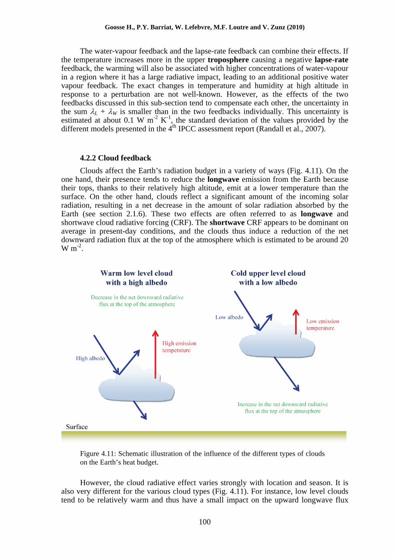
The vertical variations of the temperature change also have a climatic effect through the lapse-rate feedback λL. For instance, the models predict enhanced warming in the upper troposphere of tropical regions in response to an increase in the concentration greenhouse gases. Because of this change in the lapse rate, the outgoing longwave radiation will be more than in an homogenous temperature change over the vertical. The system will then lose more energy, so inducing a negative feedback (Fig. 4.10). Moreover, at mid to high latitudes, more low-level warming is projected as a response to the positive radiative warming, providing a positive feedback (Fig. 4.10). The global mean value of λL thus depends on the relative magnitude of those two opposite effects. On average, the influence of the tropics dominates, leading to a value of λL of around -0.8 W m-2 K-1 (Soden and Held, 2006) in recent models driven by a doubling of the CO2 concentration in the atmosphere.

Figure 4.10: Schematic representation of positive and negative lapse-rate feedbacks.

99


The water-vapour feedback and the lapse-rate feedback can combine their effects. If the temperature increases more in the upper troposphere causing a negative lapse-rate feedback, the warming will also be associated with higher concentrations of water-vapour in a region where it has a large radiative impact, leading to an additional positive water vapour feedback. The exact changes in temperature and humidity at high altitude in response to a perturbation are not well-known. However, as the effects of the two feedbacks discussed in this sub-section tend to compensate each other, the uncertainty in the sum λL + λW is smaller than in the two feedbacks individually. This uncertainty is estimated at about 0.1 W m-2 K-1, the standard deviation of the values provided by the different models presented in the 4th IPCC assessment report (Randall et al., 2007).

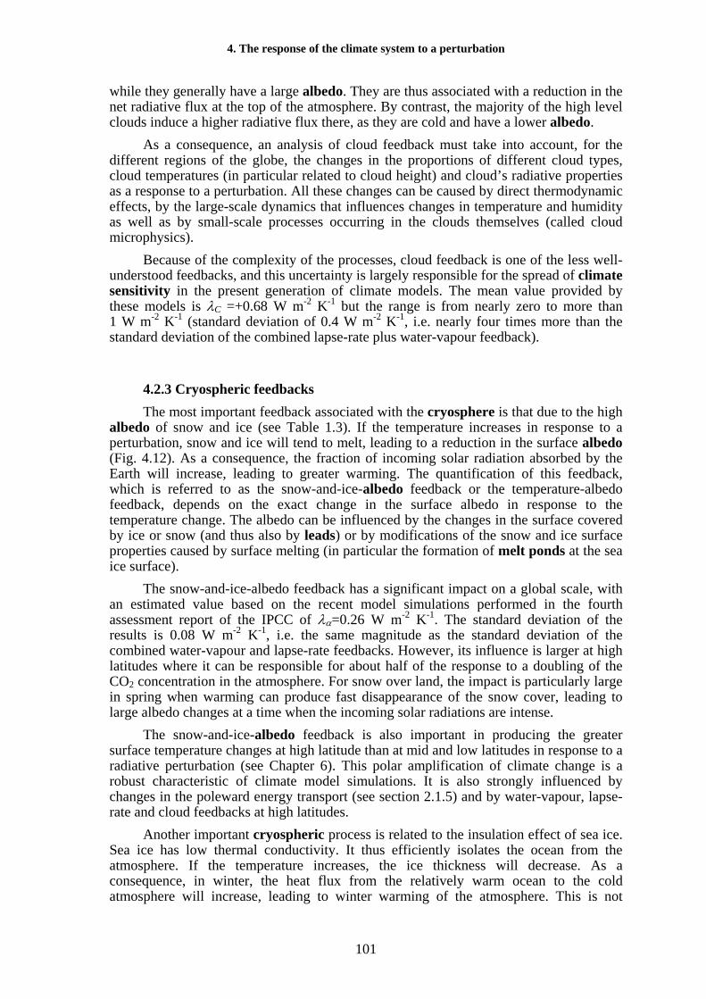
4.2.2 Cloud feedback Clouds affect the Earth’s radiation budget in a variety of ways (Fig. 4.11). On the

one hand, their presence tends to reduce the longwave emission from the Earth because their tops, thanks to their relatively high altitude, emit at a lower temperature than the surface. On the other hand, clouds reflect a significant amount of the incoming solar radiation, resulting in a net decrease in the amount of solar radiation absorbed by the Earth (see section 2.1.6). These two effects are often referred to as longwave and shortwave cloud radiative forcing (CRF). The shortwave CRF appears to be dominant on average in present-day conditions, and the clouds thus induce a reduction of the net downward radiation flux at the top of the atmosphere which is estimated to be around 20 W m-2.

Figure 4.11: Schematic illustration of the influence of the different types of clouds on the Earth’s heat budget.

However, the cloud radiative effect varies strongly with location and season. It is also very different for the various cloud types (Fig. 4.11). For instance, low level clouds tend to be relatively warm and thus have a small impact on the upward longwave flux

100


while they generally have a large albedo. They are thus associated with a reduction in the net radiative flux at the top of the atmosphere. By contrast, the majority of the high level clouds induce a higher radiative flux there, as they are cold and have a lower albedo.

As a consequence, an analysis of cloud feedback must take into account, for the different regions of the globe, the changes in the proportions of different cloud types, cloud temperatures (in particular related to cloud height) and cloud’s radiative properties as a response to a perturbation. All these changes can be caused by direct thermodynamic effects, by the large-scale dynamics that influences changes in temperature and humidity as well as by small-scale processes occurring in the clouds themselves (called cloud microphysics).

Because of the complexity of the processes, cloud feedback is one of the less well-understood feedbacks, and this uncertainty is largely responsible for the spread of climate sensitivity in the present generation of climate models. The mean value provided by these models is λC =+0.68 W m-2 K-1 but the range is from nearly zero to more than 1 W m-2 K-1 (standard deviation of 0.4 W m-2 K-1, i.e. nearly four times more than the standard deviation of the combined lapse-rate plus water-vapour feedback).

4.2.3 Cryospheric feedbacks The most important feedback associated with the cryosphere is that due to the high

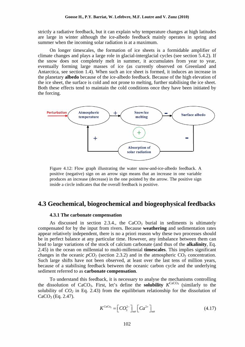
albedo of snow and ice (see Table 1.3). If the temperature increases in response to a perturbation, snow and ice will tend to melt, leading to a reduction in the surface albedo (Fig. 4.12). As a consequence, the fraction of incoming solar radiation absorbed by the Earth will increase, leading to greater warming. The quantification of this feedback, which is referred to as the snow-and-ice-albedo feedback or the temperature-albedo feedback, depends on the exact change in the surface albedo in response to the temperature change. The albedo can be influenced by the changes in the surface covered by ice or snow (and thus also by leads) or by modifications of the snow and ice surface properties caused by surface melting (in particular the formation of melt ponds at the sea ice surface).

The snow-and-ice-albedo feedback has a significant impact on a global scale, with an estimated value based on the recent model simulations performed in the fourth assessment report of the IPCC of λα=0.26 W m-2 K-1. The standard deviation of the results is 0.08 W m-2 K-1, i.e. the same magnitude as the standard deviation of the combined water-vapour and lapse-rate feedbacks. However, its influence is larger at high latitudes where it can be responsible for about half of the response to a doubling of the CO2 concentration in the atmosphere. For snow over land, the impact is particularly large in spring when warming can produce fast disappearance of the snow cover, leading to large albedo changes at a time when the incoming solar radiations are intense.

The snow-and-ice-albedo feedback is also important in producing the greater surface temperature changes at high latitude than at mid and low latitudes in response to a radiative perturbation (see Chapter 6). This polar amplification of climate change is a robust characteristic of climate model simulations. It is also strongly influenced by changes in the poleward energy transport (see section 2.1.5) and by water-vapour, lapse-rate and cloud feedbacks at high latitudes.

Another important cryospheric process is related to the insulation effect of sea ice. Sea ice has low thermal conductivity. It thus efficiently isolates the ocean from the atmosphere. If the temperature increases, the ice thickness will decrease. As a consequence, in winter, the heat flux from the relatively warm ocean to the cold atmosphere will increase, leading to winter warming of the atmosphere. This is not

101


strictly a radiative feedback, but it can explain why temperature changes at high latitudes are large in winter although the ice-albedo feedback mainly operates in spring and summer when the incoming solar radiation is at a maximum.

On longer timescales, the formation of ice sheets is a formidable amplifier of climate changes and plays a large role in glacial-interglacial cycles (see section 5.4.2). If the snow does not completely melt in summer, it accumulates from year to year, eventually forming large masses of ice (as currently observed on Greenland and Antarctica, see section 1.4). When such an ice sheet is formed, it induces an increase in the planetary albedo because of the ice-albedo feedback. Because of the high elevation of the ice sheet, the surface is cold and not prone to melting, further stabilising the ice sheet. Both these effects tend to maintain the cold conditions once they have been initiated by the forcing.

Figure 4.12: Flow graph illustrating the water snow-and-ice-albedo feedback. A positive (negative) sign on an arrow sign means that an increase in one variable produces an increase (decrease) in the one pointed by the arrow. The positive sign inside a circle indicates that the overall feedback is positive.

4.3 Geochemical, biogeochemical and biogeophysical feedbacks

4.3.1 The carbonate compensation As discussed in section 2.3.4., the CaCO3 burial in sediments is ultimately

compensated for by the input from rivers. Because weathering and sedimentation rates appear relatively independent, there is no a priori reason why these two processes should be in perfect balance at any particular time. However, any imbalance between them can lead to large variations of the stock of calcium carbonate (and thus of the alkalinity, Eq. 2.45) in the ocean on millennial to multi-millennial timescales. This implies significant changes in the oceanic pCO2 (section 2.3.2) and in the atmospheric CO2 concentration. Such large shifts have not been observed, at least over the last tens of million years, because of a stabilising feedback between the oceanic carbon cycle and the underlying sediment referred to as carbonate compensation.

To understand this feedback, it is necessary to analyse the mechanisms controlling the dissolution of CaCO3. First, let’s define the solubility KCaCO3 (similarly to the solubility of CO2 in Eq. 2.43) from the equilibrium relationship for the dissolution of CaCO3 (Eq. 2.47).

3 2 23

CaCo

sat satK CO Ca− +⎡ ⎤ ⎡ ⎤= ⎣ ⎦ ⎣ ⎦ (4.17)

102


where 23 sat

CO −⎡ ⎤⎣ ⎦ and 2

satCa +⎡ ⎤⎣ ⎦

2Ca

are the concentrations when the equilibrium between

CaCO3 and the dissolved ions is achieved, i.e at saturation. If at one location in the ocean the product 2

3CO − +⎡ ⎤⎣ ⎦⎡ ⎤⎣ ⎦

23CO −

is higher than KCaCO3, the water is said to be supersaturated with respect to CaCO3. If the product is smaller than KCaCO3, the water is undersaturated. As the variations of the concentration in Ca2+ are much smaller than the variations in the concentration of , saturation is mainly influenced by 2

3CO −⎡ ⎤⎣ ⎦ .

Observations show that the concentration of 23CO − decreases with depth (inset of

Fig. 4.13). The downward transport of inorganic carbon by the soft tissue pump and the carbonate pump might suggest the opposite. However, we must recall that the alkalinity is mainly influenced by the concentration of bicarbonate and carbonate ions (see the discussion of Eq. 2.45). Neglecting the small contribution of carbonic acid, Alk can be approximated by:

23 2Alk HCO CO3− −⎡ ⎤ ⎡+ ⎤⎣ ⎦ ⎣ ⎦

3

(4.18)

If we also neglect the influence of the carbonic acid on the DIC, we can write:

23DIC HCO CO− −⎡ ⎤ ⎡ ⎤+⎣ ⎦ ⎣ ⎦ (4.19)

This leads to

23CO Alk DIC−⎡ ⎤ −⎣ ⎦ (4.20)

The dissolution of calcium carbonate releases 23CO − directly. This is consistent

with Eq. 4.20 as the dissolution of 1 mole of CaCO3 increases Alk by 2 and DIC by 1. By contrast, the remineralisation of organic matter mainly affects the DIC, producing a decrease in 2

3CO −⎡⎣ ⎤⎦ , according to Eq. 4.20. In the present oceanic conditions, the influence of the soft tissue pump appears to dominate, leading to the observed decrease of at depth. As the solubility of CaCO3 increases in the deep ocean, mainly because of its pressure dependence, the upper ocean tends to be supersaturated while the deep ocean is undersaturated. The depth at which those two regions are separated is called the saturation horizon (inset of Fig. 4.13).

23CO −

Some of the CaCO3 that leaves the surface layer is dissolved in the ocean water column, but a significant part is transferred to the sediment. There, a fraction of the CaCO3 is dissolved and reinjected into the ocean, the rest being buried in the sediment on a long timescale. In order to describe those processes, the lysocline is defined as the depth up to which CaCO3 in sediments is subject to very little dissolution while below the Calcite Compensation Depth (CCD) nearly all the calcite is lost from the sediment by dissolution. The CCD is then the depth at which the input from sedimentation exactly balances the loss from dissolving calcite at the top of the sediment. The region between the lysocline and the CCD is called the transition zone (Fig. 4.13).

The position of the transition zone depends on several factors, in particular the presence of organic material in the sediment. It is significantly influenced by the

103


saturation of the waters above the sediment: if they are undersaturated, dissolution in the sediment tends to be relatively high, but if the waters are supersaturated dissolution is very low (as in the upper ocean). If the saturation horizon changes, the position of the transition zone is modified and the regions of the ocean where CaCO3 is preserved in sediment change.

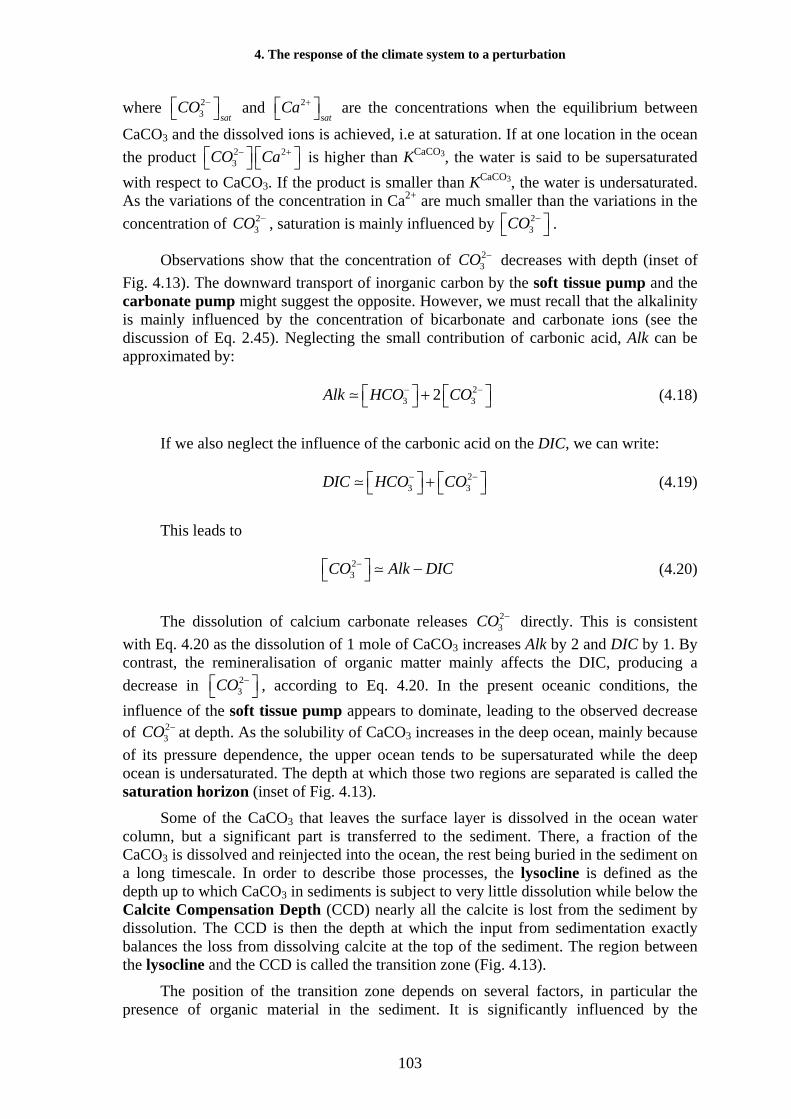
Figure 4.13: a) The current CaCO3 budget in PgC yr-1. 0.13 PgC yr-1 comes from the rivers and about 1.0 PgC yr-1 of CaCO3 is produced in the ocean, of which 0.5 PgC yr-1 is dissolved in the water column and 0.5 PgC yr-1 is transferred to the sediment. Of the CaCO3 transferred to the sediment, 0.37 PgC yr-1 is dissolved and goes back to the deep ocean, and 0.13 PgC yr-1 accumulates in the sediment, so balancing the input from rivers. b) If the river input doubles, the saturation horizon deepens, so that less CaCO3 dissolves and more accumulates in the sediment a new balance is reached. Insets show the vertical profiles of CO2

3−⎡ ⎤⎣ ⎦ , solubility and

the saturation horizon. Figure from Sarmiento and Gruber (2006). Reprinted by permission of Princeton University Press.

104


Those shifts in the saturation horizon are responsible for the stabilisation of the ocean alkalinity. Imagine for instance that the input of CaCO3 from the rivers doubles because of more intense weathering on continents (Fig. 4.13). The alkalinity of the ocean will increase. As a consequence the 2

3CO −⎡ ⎤⎣ ⎦ will increase (Eq. 4.20) and the saturation horizon will fall. The fraction of the ocean floor which is in contact with undersaturated waters will increase. This would lead to a higher accumulation of CaCO3 in sediment and thus a larger net flux of CaCO3 from the ocean to the sediment. This fall in the saturation horizon will continue until a new balance is achieved between the increased input of CaCO3 from the rivers and the greater accumulation in the sediment.

This feedback limits the amplitude of the variations in alkalinity in the ocean and thus of the atmospheric CO2 concentration. For instance, it has been estimated that, in the example presented above, a doubling of the river input of CaCO3 would only lead to a change of the order of 30 ppm in the concentration of atmospheric CO2.

4.3.2 Interaction between plate tectonics, climate and the carbon cycle

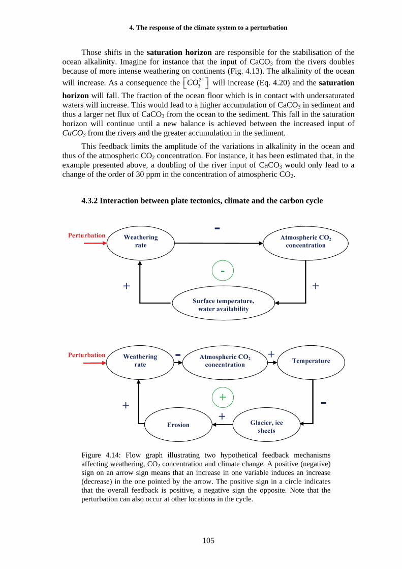
Figure 4.14: Flow graph illustrating two hypothetical feedback mechanisms affecting weathering, CO2 concentration and climate change. A positive (negative) sign on an arrow sign means that an increase in one variable induces an increase (decrease) in the one pointed by the arrow. The positive sign in a circle indicates that the overall feedback is positive, a negative sign the opposite. Note that the perturbation can also occur at other locations in the cycle.

105


The chemical weathering of rocks (e.g., Eq. 2.49) is influenced by a large number of processes. In particular, high temperatures and the availability of water at the surface tend to induce higher weathering rates, at least for some rocks such as the basalts. As the weathering consumes atmospheric CO2 (see section 2.3.4), this can potentially lead to a negative feedback that can regulate the long term variations in the atmospheric CO2 concentration (Fig. 4.14). For example, more intense tectonic activity might cause the uplift of a large amount of calcium-silicate rocks to the surface, leading to an increase in the weathering rate. The atmospheric CO2 concentration would then decrease, producing a general cooling of the climate system. This would lead to lower evaporation and so less precipitation and lower water availability. These climate changes would then reduce the weathering rates, so moderating the initial perturbation.

In a second hypothesis, we can postulate that the rate of weathering is mainly influenced by mechanical erosion, which increases the exposition of fresh, new rocks to the atmosphere and these can then be more efficiently altered. If the temperature decreases because of a higher rate of weathering, glaciers and ice sheets can cover a larger surface. As they are very active erosion agents, this would increase the mechanical weathering and so the chemical weathering, amplifying the initial perturbation (Fig. 4.14).

Although they both appear reasonable, these two feedback mechanisms are still being debated. Their exact role, if any, in the variations of CO2 concentration on time scales of hundreds of thousands to millions of years is still uncertain.

4.3.3 Interactions between climate and the terrestrial biosphere The terrestrial biosphere plays an important role in the global carbon cycle (section

2.3.3). Changes in the geographical distribution of the different biomes, induced by climate modifications, can modify carbon storage on land and so have an impact on the atmospheric concentration of CO2. This can potentially lead to feedbacks that are commonly referred to as biogeochemical feedbacks as they involve the interactions between climate, biological activity and the biogeochemical cycle of an important chemical element on Earth (the carbon).

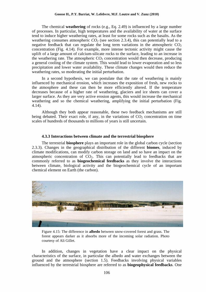
Figure 4.15: The difference in albedo between snow-covered forest and grass. The forest appears darker as it absorbs more of the incoming solar radiation. Photo courtesy of Ali Gillet.

In addition, changes in vegetation have a clear impact on the physical characteristics of the surface, in particular the albedo and water exchanges between the ground and the atmosphere (section 1.5). Feedbacks involving physical variables influenced by the terrestrial biosphere are referred to as biogeophysical feedbacks. One

106


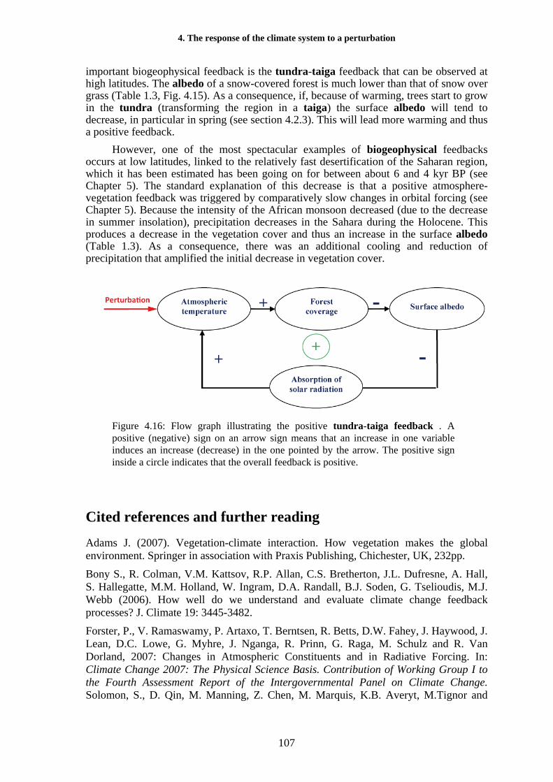
important biogeophysical feedback is the tundra-taiga feedback that can be observed at high latitudes. The albedo of a snow-covered forest is much lower than that of snow over grass (Table 1.3, Fig. 4.15). As a consequence, if, because of warming, trees start to grow in the tundra (transforming the region in a taiga) the surface albedo will tend to decrease, in particular in spring (see section 4.2.3). This will lead more warming and thus a positive feedback.

However, one of the most spectacular examples of biogeophysical feedbacks occurs at low latitudes, linked to the relatively fast desertification of the Saharan region, which it has been estimated has been going on for between about 6 and 4 kyr BP (see Chapter 5). The standard explanation of this decrease is that a positive atmosphere-vegetation feedback was triggered by comparatively slow changes in orbital forcing (see Chapter 5). Because the intensity of the African monsoon decreased (due to the decrease in summer insolation), precipitation decreases in the Sahara during the Holocene. This produces a decrease in the vegetation cover and thus an increase in the surface albedo (Table 1.3). As a consequence, there was an additional cooling and reduction of precipitation that amplified the initial decrease in vegetation cover.

Figure 4.16: Flow graph illustrating the positive tundra-taiga feedback . A positive (negative) sign on an arrow sign means that an increase in one variable induces an increase (decrease) in the one pointed by the arrow. The positive sign inside a circle indicates that the overall feedback is positive.

Cited references and further reading

Adams J. (2007). Vegetation-climate interaction. How vegetation makes the global environment. Springer in association with Praxis Publishing, Chichester, UK, 232pp.

Bony S., R. Colman, V.M. Kattsov, R.P. Allan, C.S. Bretherton, J.L. Dufresne, A. Hall, S. Hallegatte, M.M. Holland, W. Ingram, D.A. Randall, B.J. Soden, G. Tselioudis, M.J. Webb (2006). How well do we understand and evaluate climate change feedback processes? J. Climate 19: 3445-3482.

Forster, P., V. Ramaswamy, P. Artaxo, T. Berntsen, R. Betts, D.W. Fahey, J. Haywood, J. Lean, D.C. Lowe, G. Myhre, J. Nganga, R. Prinn, G. Raga, M. Schulz and R. Van Dorland, 2007: Changes in Atmospheric Constituents and in Radiative Forcing. In: Climate Change 2007: The Physical Science Basis. Contribution of Working Group I to the Fourth Assessment Report of the Intergovernmental Panel on Climate Change. Solomon, S., D. Qin, M. Manning, Z. Chen, M. Marquis, K.B. Averyt, M.Tignor and

107


108

H.L. Miller (Eds.). Cambridge University Press, Cambridge, United Kingdom and New York, NY, USA.

Gao C., A. Robock and C. Ammann. (2008). Volcanic forcing of climate over the past 1500 years: an improved ice core-based index for climate models. Journal of Geophysical Research 113, D23111.

Hansen J., M. Sato and R.Ruedy (1997). Radiative forcing and climate response. J. Geophys. Res. 102 (D6): 6831-6884.

Hartmann D.L. (1994). Global physical climatology. International Geophysics series, volume 56. Academic Press, 412 pp.

IPCC (2007). Climate Change 2007: The Physical Basis. Contribution of Working Group I to the Fourth Assessment Report of the Intergovernmental Panel on Climate Change. Solomon, S., Qin, D., Manning, M., Chen, Z., Marquis, M., Averyt, K.B., Tignor, M., and Miller H.L. (Eds.), Cambridge Univ. Press, Cambridge, U.K. and New York, U.S.A., 996 pp.

Koch D., S. Menon, A.Del Genio, R. Ruedy, I.A. Alienov and G.A. Schmidt (2008). Distinguishing aerosol impacts on climate over the past century. Journal of Climate 22, 2659-2677.

Ramankutty N. and J.A., Foley 1999. Estimating historical changes in global land cover: croplands from 1700 to 1992, Global. Biogeochemical Cycles 13, 4:997-1027.

Randall, D.A., R.A. Wood, S. Bony, R. Colman, T. Fichefet, J. Fyfe, V. Kattsov, A. Pitman, J. Shukla, A. Noda, J. Srinivasan, R.J. Stouffer, A. Sumi and K.E. Taylor (2007). Climate models and their evaluation. In: Climate Change 2007: The Physical Science Basis. Contribution of Working Group I to the Fourth Assessment Report of the Intergovernmental Panel on Climate Change. Solomon, S., D. Qin, M. Manning, Z. Chen, M. Marquis, K.B. Averyt, M. Tignor and H.L. Miller (eds.). Cambridge University Press, Cambridge, United Kingdom and New York, NY, USA.

Rotaru M., J. Gaillardet, M. Steinberg and J. Trichet (2006). Les climats passés de la terre. Société Géologique de France, Vuibert, 195pp.

Sarmiento G.L and N. Gruber (2006). Ocean biogeochemical dynamics. Princeton University Press, 503pp.

Soden B.F. and I.M. Held (2006). An assessment of climate feedbacks in coupled ocean-atmosphere models. J. Climate, 19, 14, 3354-3360.

Wallace J.M. and P.V. Hobbs (2006). Atmospheric science: an introductory survey (2nd edition). International Geophysics Series 92, Associated press, 484pp. Wang Y.M., J.L. Lean and N.R. Sheeley (2005). Modeling the sun's magnetic field and irradiance since 1713. Astrophysical Journal 625, 1, 522-538

Exercises

Exercises are available on the textbook website (http://www.climate.be/textbook) and on iCampus for registered students.

Documents

Chapter 4. The response of the climate system to a ... · PDF fileThe response of the climate system to a perturbation . 4.1 Climate forcing and ... The response of the climate system