Embed Size (px)
Citation preview

Chapter 4Chapter 4
Theoretical Theoretical BackgroundBackground
4.1 Convergence4.1 ConvergenceQUESTIONS? Under what conditions the numerical solution
will coincide with the exact solution? What guarantee the numerical solution will be
close to the exact solution of the PDE? Consistency – discretization solution process can
be reversed, through a Taylor series expansion, to recover the original PDEs
Stability – solution algorithm must be stable Convergence – solution of the discretization
equations (approximate solution) approaches the exact solution for the original PDE when x 0 and t 0 (grid refinement)
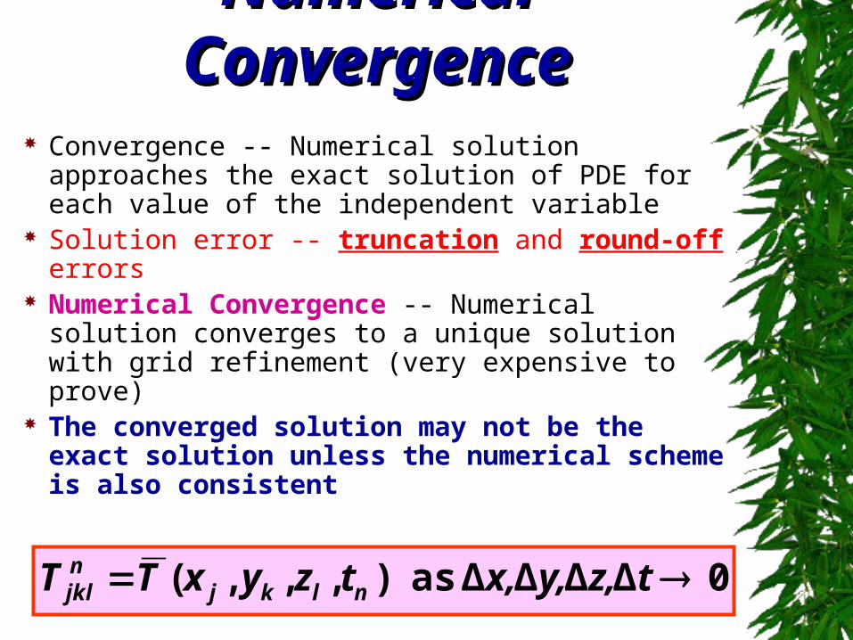
Numerical ConvergenceNumerical Convergence Convergence -- Numerical solution approaches
the exact solution of PDE for each value of the independent variable
Solution error -- truncation and round-off errors Numerical Convergence -- Numerical solution
converges to a unique solution with grid refinement (very expensive to prove)
The converged solution may not be the exact solution unless the numerical scheme is also consistent
0ΔΔΔΔ as ),,,( tz,y,x,tzyxTT nlkjnjkl
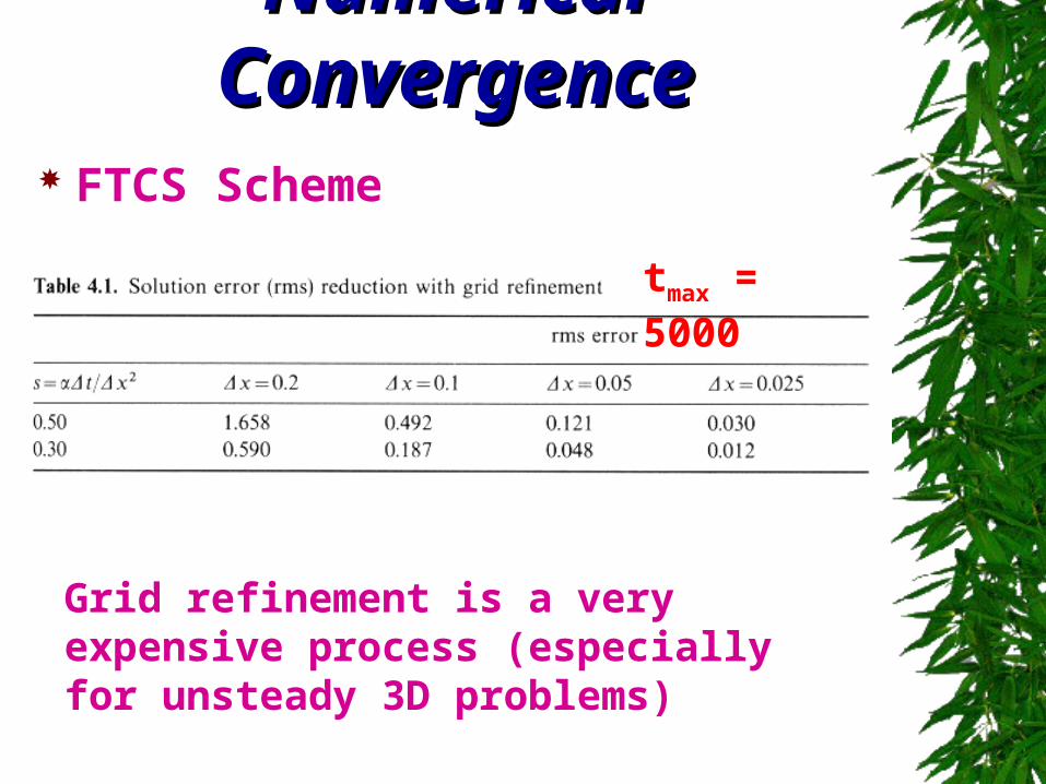
Numerical ConvergenceNumerical Convergence FTCS Scheme
tmax = 5000
Grid refinement is a very expensive process (especially for unsteady 3D problems)
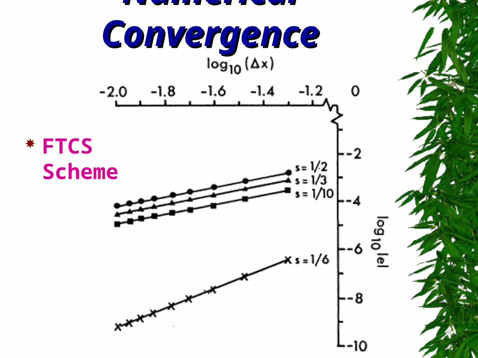
Numerical ConvergenceNumerical Convergence
FTCS Scheme
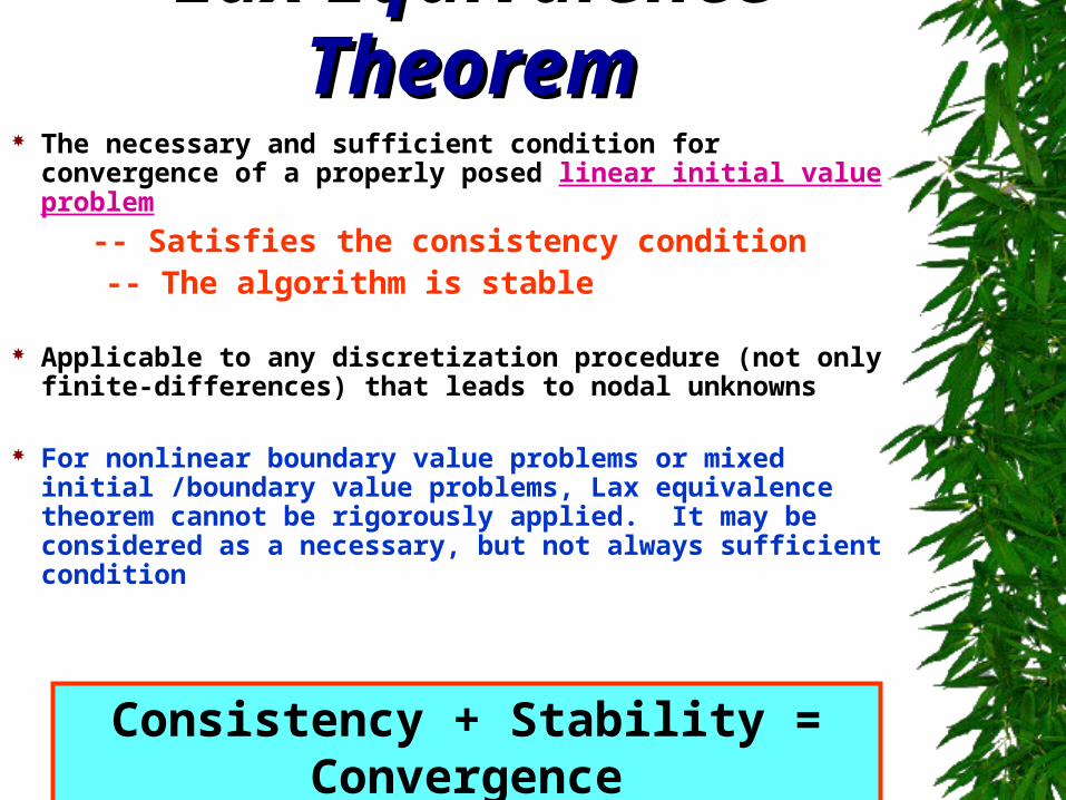
Lax Equivalence TheoremLax Equivalence Theorem The necessary and sufficient condition for convergence of a
properly posed linear initial value problem
-- Satisfies the consistency condition -- The algorithm is stable
Applicable to any discretization procedure (not only finite-differences) that leads to nodal unknowns
For nonlinear boundary value problems or mixed initial /boundary value problems, Lax equivalence theorem cannot be rigorously applied. It may be considered as a necessary, but not always sufficient condition
Consistency + Stability = Convergence
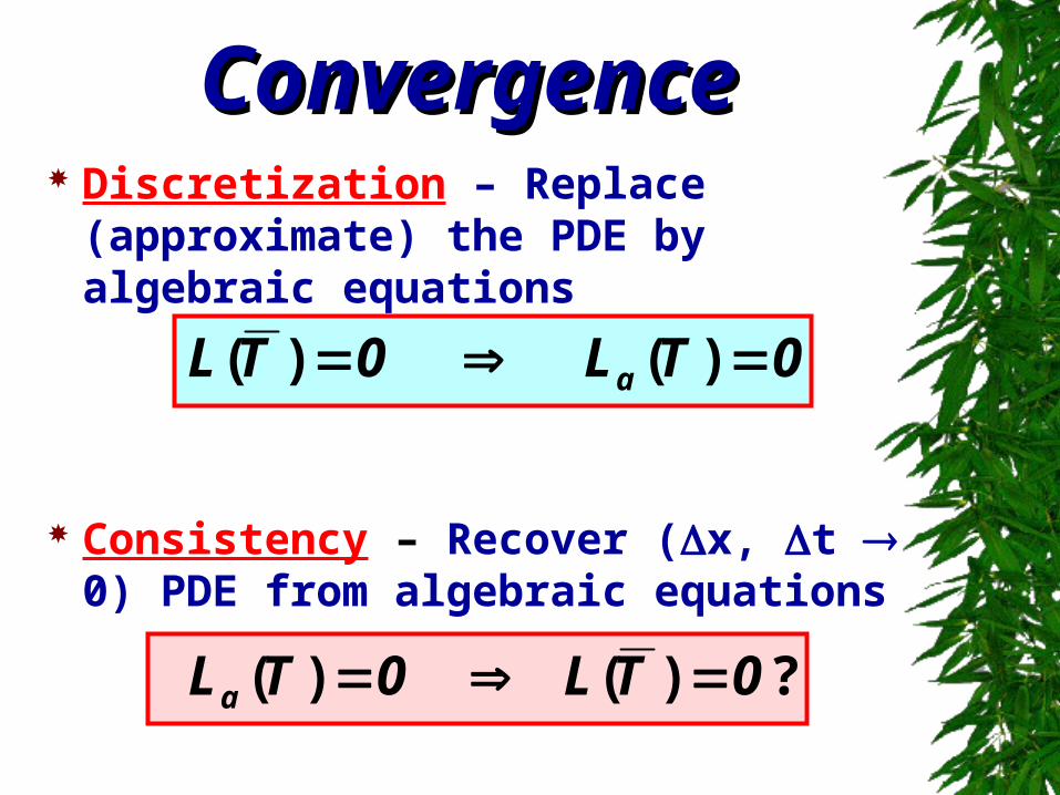
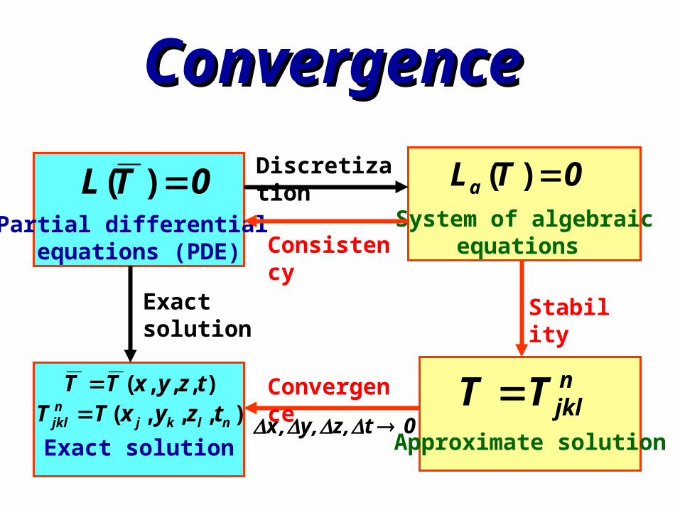
ConvergenceConvergence Discretization – Replace (approximate)
the PDE by algebraic equations
Consistency – Recover (x, t 0) PDE from algebraic equations
0TL0TL a )( )(
? )( )( 0TL0TLa
Exact solution
System of algebraicequations
Partial differential equations (PDE)
ConvergenceConvergence
0TL )( 0TLa )(
),,,(),,,(
nlkjnjkl tzyxTT
tzyxTT
Approximate solution
njklTT
Discretization
Consistency
Convergence
0t,z,y,x
StabilityExact solution
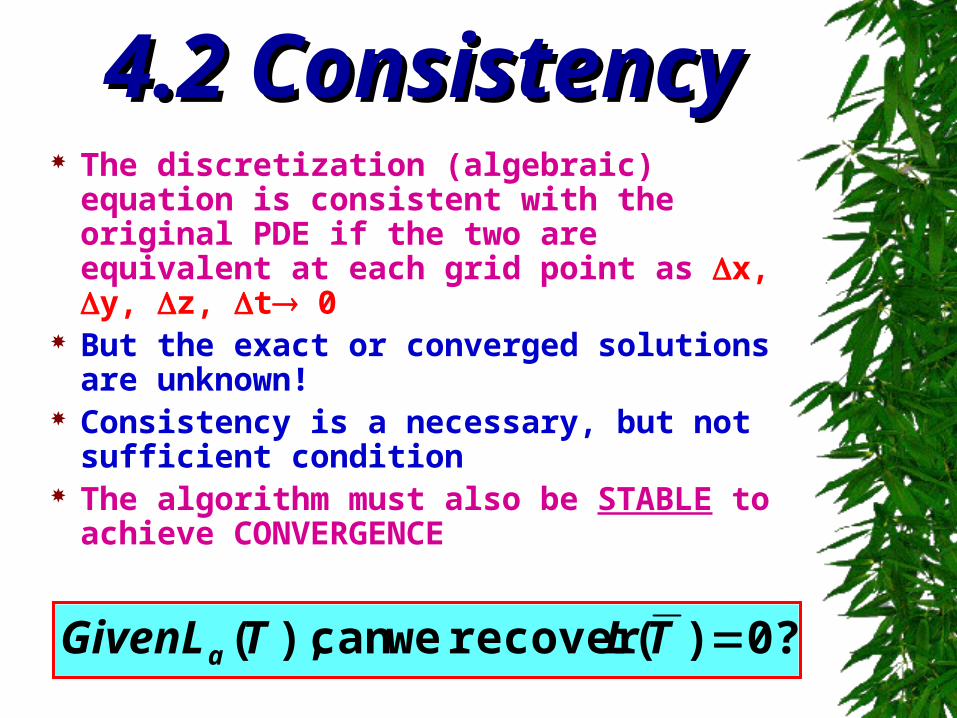
4.2 Consistency4.2 Consistency The discretization (algebraic) equation is
consistent with the original PDE if the two are equivalent at each grid point as x, y, z, t 0
But the exact or converged solutions are unknown!
Consistency is a necessary, but not sufficient condition
The algorithm must also be STABLE to achieve CONVERGENCE
0?)(recover we can ),( TLTLGiven a
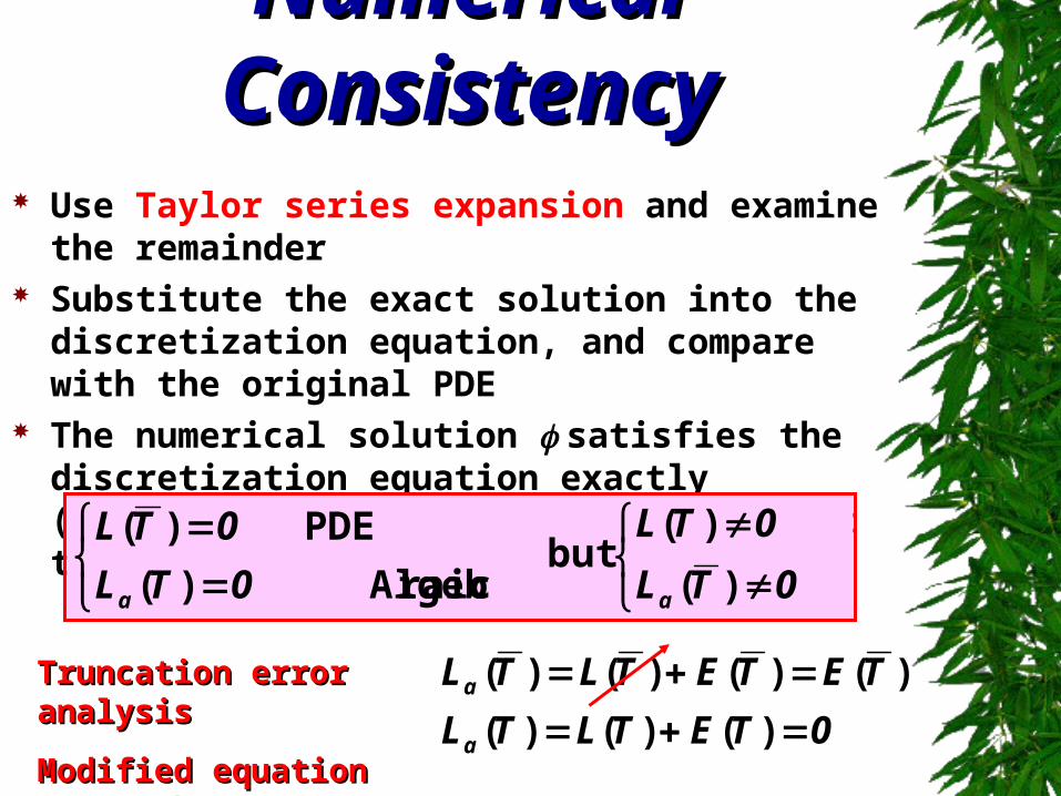
Numerical ConsistencyNumerical Consistency Use Taylor series expansion and examine the remainder Substitute the exact solution into the discretization
equation, and compare with the original PDE The numerical solution satisfies the discretization
equation exactly (assuming no round-off error), but not the original PDE
)(
)(but
raic Algeb)(
PDE )(
0TL
0TL
0TL
0TL
aa
0TETLTL
TETETLTL
a
a
)()()(
)()()()(Truncation error analysisTruncation error analysis
Modified equation approachModified equation approach
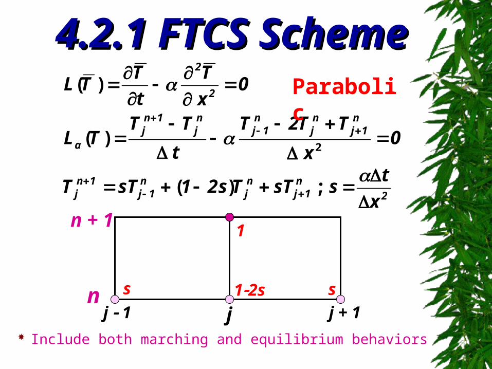
4.2.1 FTCS Scheme4.2.1 FTCS Scheme
Include both marching and equilibrium behaviors
2n
1jnj
n1j
1nj
n1j
nj
n1j
nj
1nj
a
2
2
x
tssTTs21sTT
0x
TT2T
t
TTTL
0x
T
t
TTL
; )(
)(
)(
2
Parabolic
n
n + 1
jj 1 j + 1
s s12s
1
! ! ! 2
! !
)(
2
2
n
j6
66n
j4
44n
j2
22
n
j3
33n
j2
22n
j
n1j
nj
n1j
nj
1nja
x
T
6
x
x
T
4
x
x
T
2
x
x
t
t
T
3
t
t
T
2
t
t
Tt
t
1
TT2Tx
tTT
t
1TL
FTCS SchemeFTCS Scheme
n
j4
44n
j3
33n
j2
22n
j
nj
n1j
n
j3
33n
j2
22n
j
nj
1nj
x
T
4
x
x
T
3
x
x
T
2
x
x
TxTT
t
T
3
t
t
T
2
t
t
TtTT
! ! !
! !
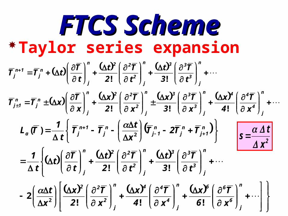
Taylor series expansion
2x
t s
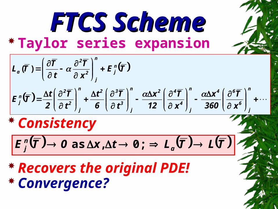
FTCS SchemeFTCS Scheme Taylor series expansion
Consistency
Recovers the original PDE! Convergence?
)(
n
j6
64n
j4
42n
j3
32n
j2
2nj
nj
n
j2
2
a
x
T
360
x
x
T
12
x
t
T
6
t
t
T
2
tTE
TEx
T
t
TTL
0; , as TLTLtx0TE anj

Numerical AccuracyNumerical Accuracy Time- and spatial-derivatives are not independent We need to know the accuracy of the discretization
equation, not just individual terms in the equation Use the PDE to relate time- and spatial-derivatives
6
63
3
3
4
42
2
2
2
2
2
2
2
2
2
2
2
2
x
T
t
T
x
T
x
T
xt
T
xx
T
tt
T
x
T
t
T
m2
m2m
m
m
x
T
t
T
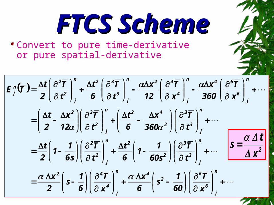
FTCS SchemeFTCS Scheme Convert to pure time-derivative or
pure spatial-derivative
n
j6
62
4n
j4
4
n
j3
3
2
2n
j2
2
n
j3
3
2
42n
j2
22
n
j6
64n
j4
42n
j3
32n
j2
2nj
x
T
60
1s
6
x
x
T
6
1s
2
x
t
T
s60
11
6
t
t
T
s6
11
2
t
t
T
360
x
6
t
t
T
12
x
2
t
x
T
360
x
x
T
12
x
t
T
6
t
t
T
2
tTE
2
2x
t s
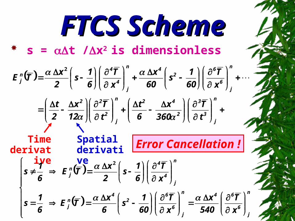
FTCS SchemeFTCS Scheme s = t /x2 is dimensionless
n
j3
3
2
42n
j2
22
n
j6
62
4n
j4
4nj
t
T
360
x
6
t
t
T
12
x
2
t
x
T
60
1s
60
x
x
T
6
1s
2
xTE
2
Time derivative
Spatial derivative
n
j6
64n
j6
62
4nj
n
j4
4nj
x
T
540
x
x
T
60
1s
6
xTE
6
1s
x
T
6
1s
2
xTE
6
1s
2
Error Cancellation !
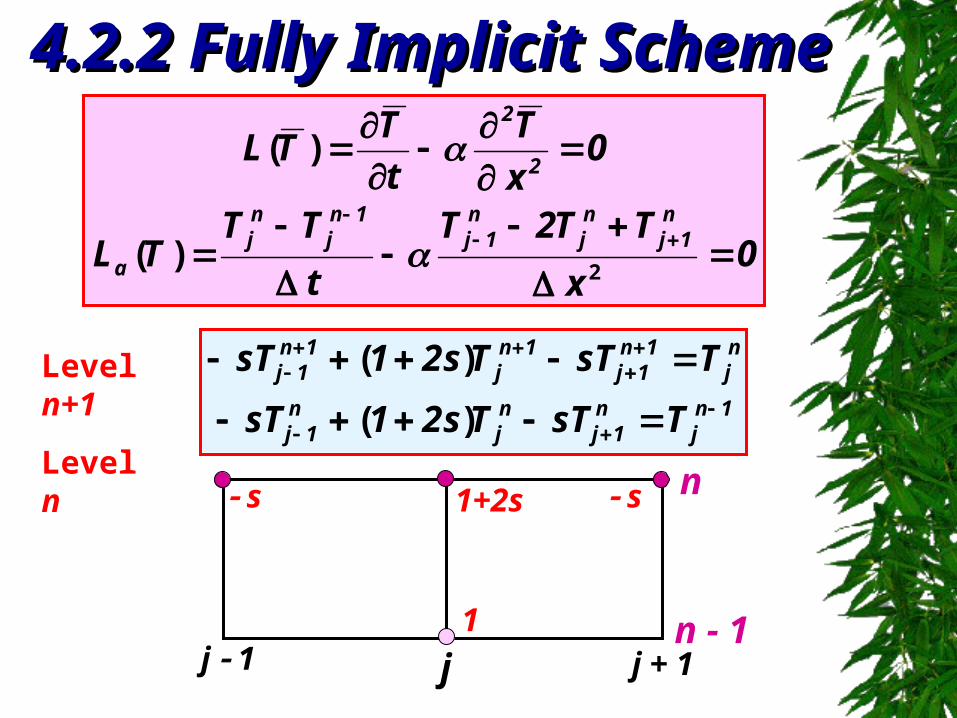
4.2.2 Fully Implicit Scheme4.2.2 Fully Implicit Scheme
0x
TT2T
t
TTTL
0x
T
t
TTL
n1j
nj
n1j
1nj
nj
a
2
2
2 )(
)(
n - 1
n
jj 1 j + 1
1nj
n1j
nj
n1j
nj
1n1j
1nj
1n1j
TsTTs21sT
TsTTs21sT
)(
)(Level n+1
Level n
s s1+2s
1
! ! !
2
! !
)(
2
2
n
j6
66n
j4
44n
j2
22
n
j3
33n
j2
22n
j
n1j
nj
n1j
1nj
nja
x
T
6
x
x
T
4
x
x
T
2
x
x
t
t
T
3
t
t
T
2
t
t
Tt
t
1
TT2Tx
tTT
t
1TL
Fully Implicit SchemeFully Implicit Scheme
n
j4
44n
j3
33n
j2
22n
j
nj
n1j
n
j3
33n
j2
22n
j
nj
1nj
x
T
4
x
x
T
3
x
x
T
2
x
x
TxTT
t
T
3
t
t
T
2
t
t
TtTT
! ! !
! !
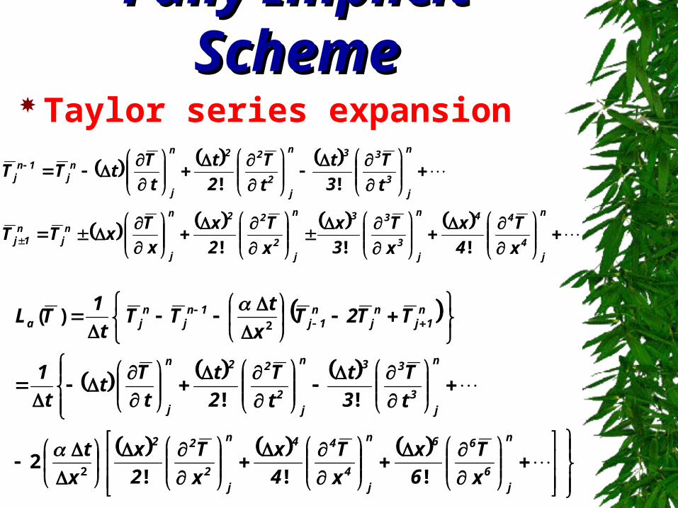
Taylor series expansion
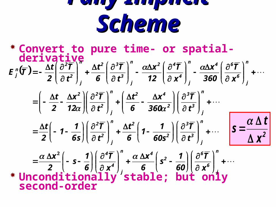
Fully Implicit SchemeFully Implicit Scheme Convert to pure time- or spatial-derivative
Unconditionally stable; but only second-order
n
j6
62
4n
j4
4
n
j3
3
2
2n
j2
2
n
j3
3
2
42n
j2
22
n
j6
64n
j4
42n
j3
32n
j2
2nj
x
T
60
1s
6
x
x
T
6
1s
2
x
t
T
s60
11
6
t
t
T
s6
11
2
t
t
T
360
x
6
t
t
T
12
x
2
t
x
T
360
x
x
T
12
x
t
T
6
t
t
T
2
tTE
2
2x
ts
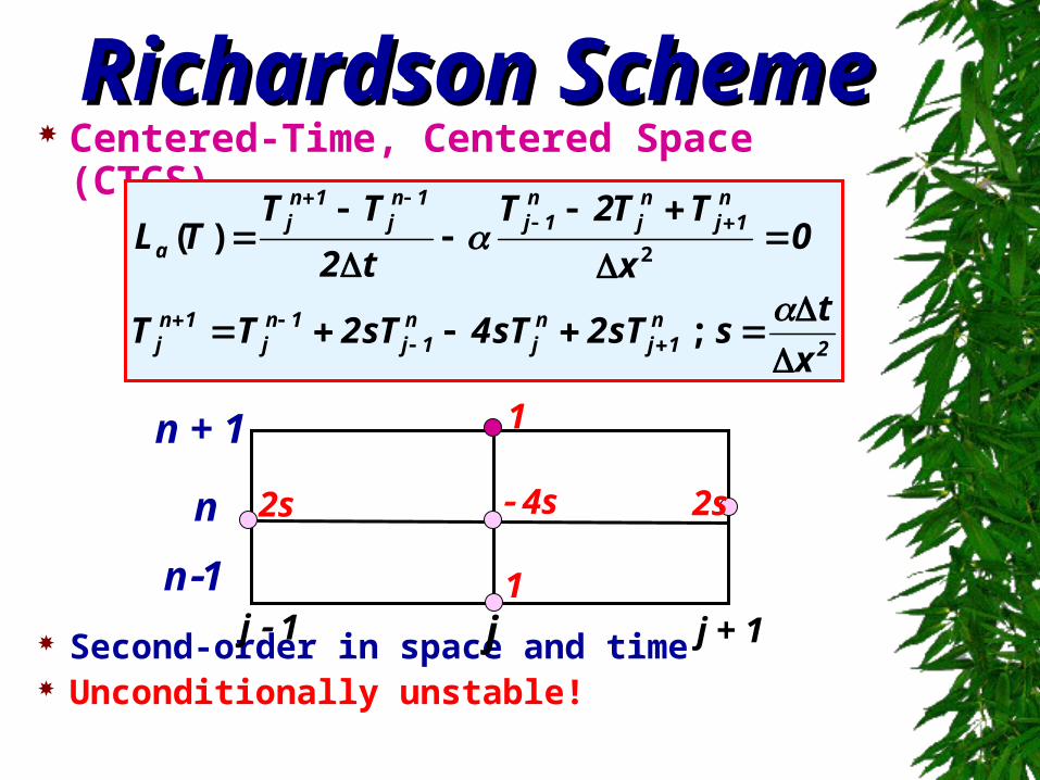
Centered-Time, Centered Space (CTCS)
Second-order in space and time Unconditionally unstable!
Richardson SchemeRichardson Scheme
2n
1jnj
n1j
1nj
1nj
n1j
nj
n1j
1nj
1nj
a
x
tssT2sT4sT2TT
0x
TT2T
t2
TTTL
;
)(2
n + 1
jj 1 j + 1
n
n1
2s 4s 2s
1
1
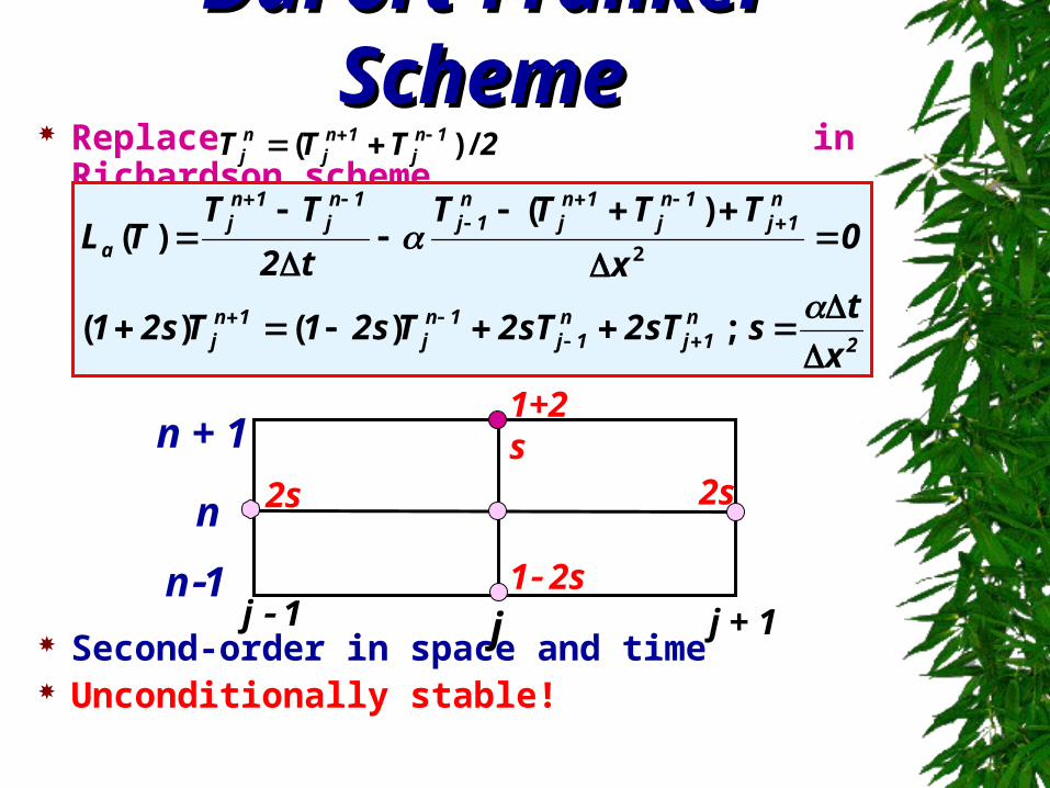
Replace in Richardson scheme
Second-order in space and time Unconditionally stable!
DuFort-Frankel SchemeDuFort-Frankel Scheme
2
n1j
n1j
1nj
1nj
n1j
1nj
1nj
n1j
1nj
1nj
a
x
tssT2sT2Ts21Ts21
0x
TTTT
t2
TTTL
; )()(
)()(
2
n + 1
jj 1 j + 1
n
n1
2s 2s
1 2s
1+2s
2TTT 1nj
1nj
nj /)(
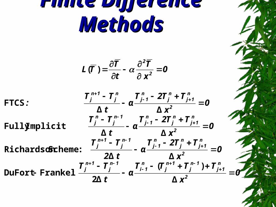
Finite Difference MethodsFinite Difference Methods
0 x
TTTTα
t
TT
0 x
TT2Tα
t2
TT
0 x
TT2Tα
t
TT
0 x
TT2Tα
t
TT :
0x
T
t
TTL
2
n1j
1nj
1nj
n1i
1nj
1nj
2
n1j
nj
n1j
1nj
1nj
2
n1j
nj
n1j
1nj
nj
2
n1j
nj
n1j
nj
1nj
2
2
Δ
)(
2Δ :FrankelDuFort
ΔΔ:Scheme Richardson
ΔΔ:Implicit Fully
ΔΔFTCS
)(
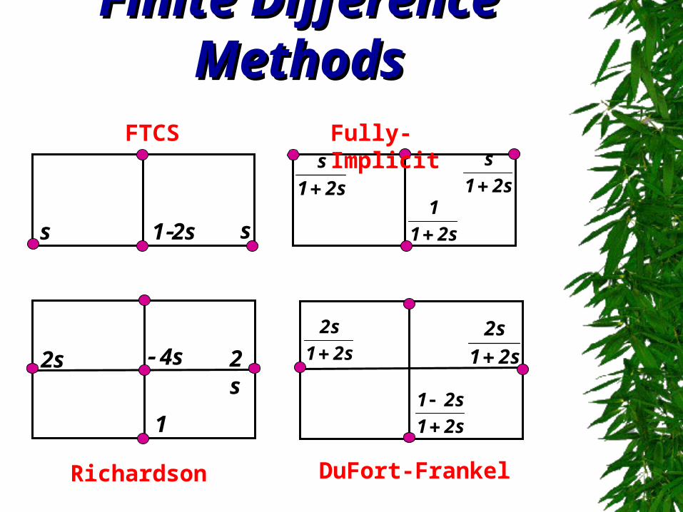
Finite Difference MethodsFinite Difference Methods
s s12s
s21
s
s21
s
s21
1
s21
s2
s21
s2
s21
s21
4s2s 2s
1
FTCS Fully-Implicit
Richardson DuFort-Frankel
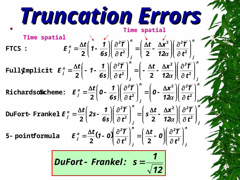
Truncation ErrorsTruncation Errors Time spatial Time spatial
n
j
2n
j
2nj
n
j
2n
j
2nj
n
i
2n
j
2nj
n
j
2n
j
2nj
n
j
2n
j
2nj
t
T0
t
t
T01
tE
t
T
12
xts
t
T
s6
1s2
tE
t
T
12
x0
t
T
s6
10
tE
t
T
12
xt
t
T
s6
11
tE
t
T
12
xt
t
T
s6
11
tE
22
2
2
2
2
2
2
2
2
2
2
2
2
2 2 :formulapoint 5
2 2 :FrankelDuFort
2 :Scheme Richardson
2 2 :Implicit Fully
2 2 :FTCS
12
1s :FrankelDuFort
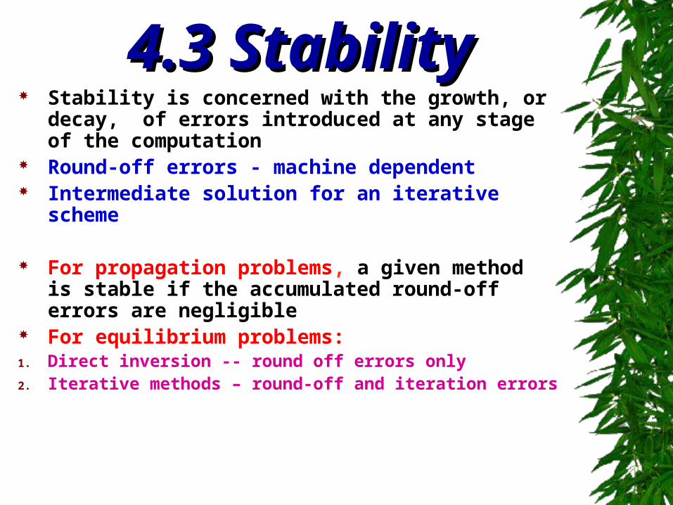
4.3 Stability4.3 Stability Stability is concerned with the growth, or decay, of
errors introduced at any stage of the computation Round-off errors - machine dependent Intermediate solution for an iterative scheme
For propagation problems, a given method is stable if the accumulated round-off errors are negligible
For equilibrium problems:1. Direct inversion -- round off errors only2. Iterative methods – round-off and iteration errors
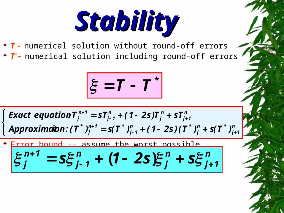
Numerical StabilityNumerical Stability T numerical solution without round-off errors T* numerical solution including round-off errors
Error bound -- assume the worst possible combinations of individual errors
*TT
n1j
*nj
*n1j
*1nj
*
n1j
nj
n1j
1nj
)T(s)T( )s21()T(s)T( :ionApproximat
sTT)s21(sTT :equation Exact
n1j
nj
n1j
1nj ss21s )(
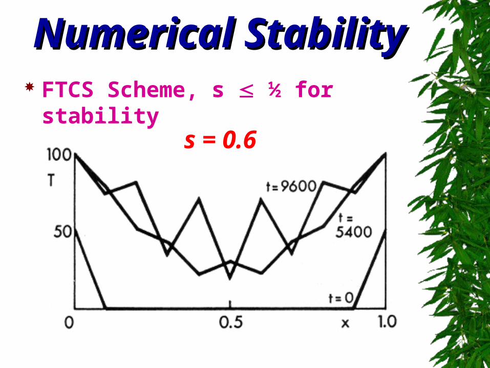
Numerical StabilityNumerical Stability FTCS Scheme, s ½ for stability
s = 0.6
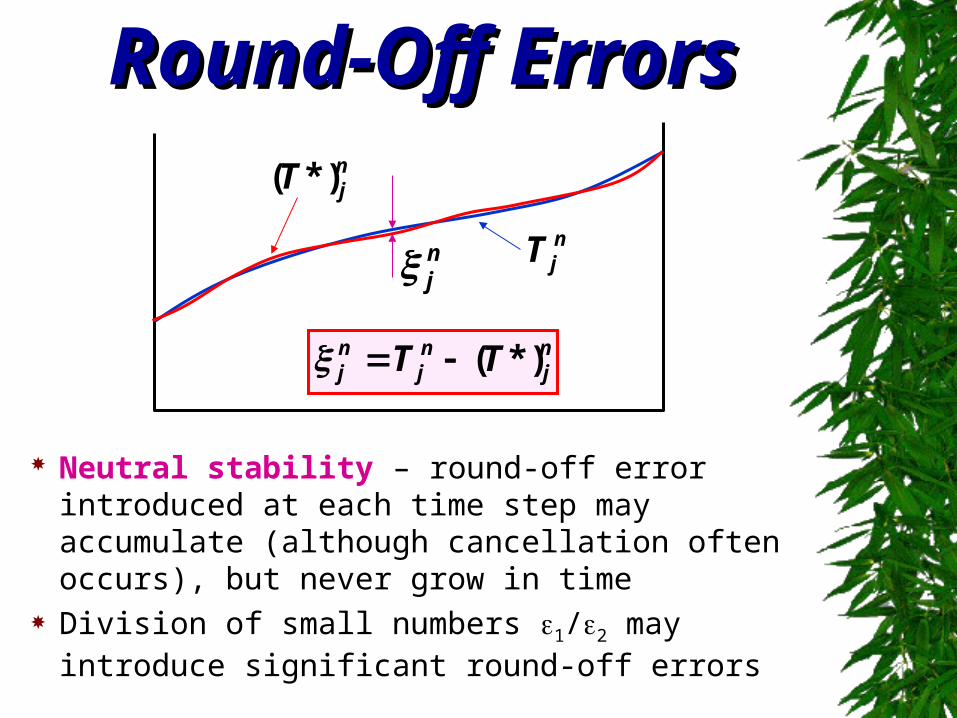
Round-Off ErrorsRound-Off Errors
Neutral stability – round-off error introduced at each time step may accumulate (although cancellation often occurs), but never grow in time
Division of small numbers 1/2 may introduce significant round-off errors
njT
njT*)(
nj
nj
nj
nj TT *)(
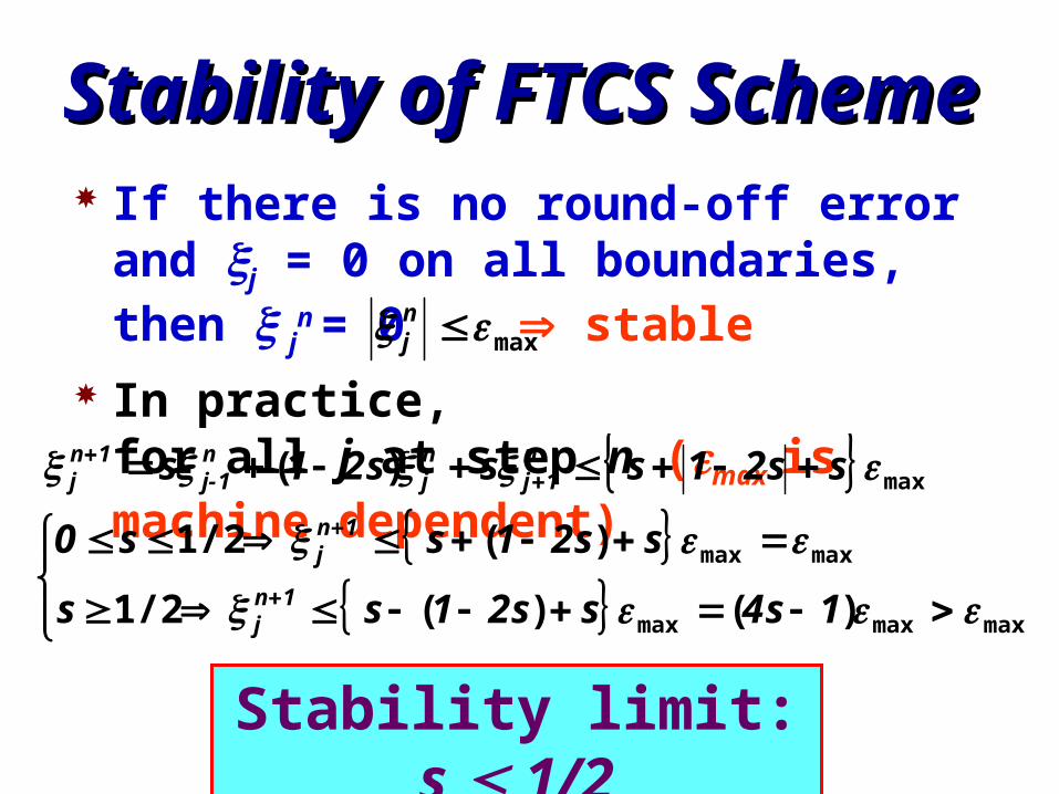
Stability of FTCS SchemeStability of FTCS Scheme If there is no round-off error and j = 0 on
all boundaries, then jn = 0 stable
In practice, for all j at step n (max is machine dependent)
maxmaxmax
maxmax
max
)( )( 1/2
)( 1/2
)(
1s4ss21ss
ss21ss0
ss21sss21s
1nj
1nj
n1j
nj
n1j-
1nj
max nj
Stability limit: s 1/2
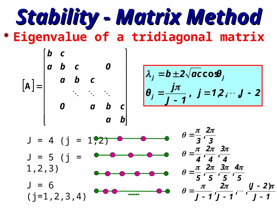
Stability - Matrix MethodStability - Matrix Method Eigenvalue of a tridiagonal matrix
ba
cba0
cba
0cba
cb
A
2J21j1J
jθ
θac2b
j
jj
,,, ,
cos
J = 4 (j = 1,2)
J = 5 (j = 1,2,3)
J = 6 (j=1,2,3,4)
In general1J
2J
1J
2
1J
5
4
5
3
5
2
5
4
3
4
2
4
3
2
3
)(,,,
,,,
,,
,
……
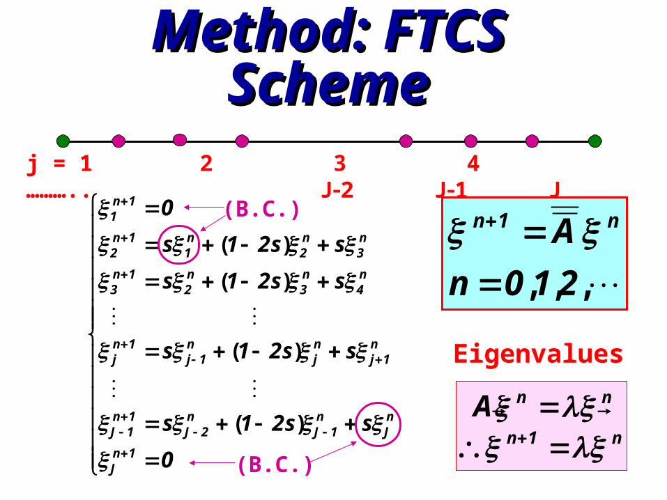
4.3.1 Matrix Method: 4.3.1 Matrix Method: FTCS SchemeFTCS Scheme
0
ss21s
ss21s
ss21s
ss21s
0
1nJ
nJ
n1J
n2J
1n1J
n1j
nj
n1j
1nj
n4
n3
n2
1n3
n3
n2
n1
1n2
1n1
)(
)(
)(
)(
(B.C.)
(B.C.)
j = 1 2 3 4 ……….. J2 J1 J
,,, 210n
A n1n
n1n
nnA
Eigenvalues
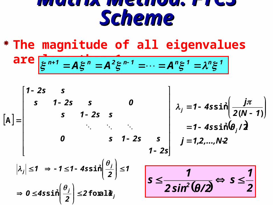
Matrix Method: FTCS SchemeMatrix Method: FTCS Scheme The magnitude of all eigenvalues are less than 1
s21
ss21s0
ss21s
0ss21s
ss21
A
AAA 1n1n1n2n1n
jj2
j2j
22
s40
12
s4111
allfor sin
sin
2,...,N-2,1j
θs41
1N2
js41
j2
2j
/2sin
)(sin
2
1s
θ/2sin2
1s
2
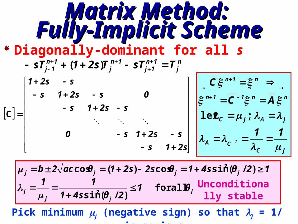
Matrix Method: Matrix Method: Fully-Implicit SchemeFully-Implicit Scheme
Diagonally-dominant for all s
s21s
ss21s0
ss21s
0ss21s
ss21
C
j
j2
jj
j2
jjj
θ12θs41
1112θs41θs2s21θac2b
allfor )/(sin
)/(sincos)(cos
nj
1n1j
1nj
1n1j TsTTs21sT
)(
Unconditionally stable
jCCA
jAjC
nn11n
n1n
11
AC
C
1
;let
Pick minimum j (negative sign) so that j = 1/ j is maximum
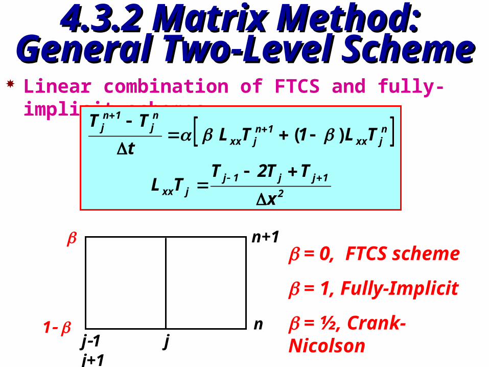
4.3.2 Matrix Method: 4.3.2 Matrix Method: General Two-Level SchemeGeneral Two-Level Scheme
Linear combination of FTCS and fully-implicit schemes
2
1jj1jjxx
njxx
1njxx
nj
1nj
x
TT2TTL
TL1TLt
TT
)(
j1 j j+1n
n+1
1
= 0, FTCS scheme
= 1, Fully-Implicit
= ½, Crank-Nicolson
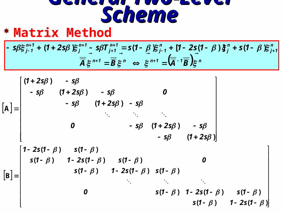
General Two-Level SchemeGeneral Two-Level Scheme Matrix Method
)(
)(
)(
)(
)(
A
s21s
ss21s0
ss21s
0ss21s
ss21
)()]([)()(
n11nn1n
n1j
nj
n1j
1n1j
1nj
1n1j
BABA
1s1s211sTss21s
)()(
)()()(
)()()(
)()()(
)()(
B
1s211s
1s1s211s0
1s1s211s
01s1s211s
1s1s21
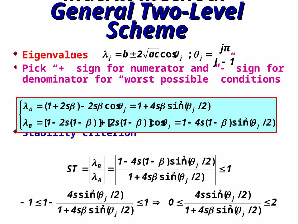
Matrix Method: Matrix Method: General Two-Level SchemeGeneral Two-Level Scheme
Eigenvalues Pick “+” sign for numerator and “” sign for
denominator for “worst possible” conditions
Stability criterion
)/(sin)(cos)]([)]([
)/(sincos)(
21s411s21s21
2s41s2s21
j2
jB
j2
jA
; cos1J
jπac2b jjj
22s41
2s401
2s41
2s411
12s41
21s41ST
j2
j2
j2
j2
j2
j2
A
B
)/(sin
)/(sin
)/(sin
)/(sin
)/(sin
)/(sin)(
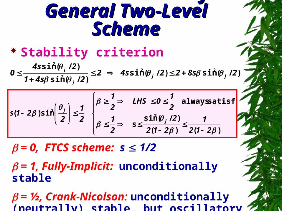
Numerical Stability:Numerical Stability:General Two-Level SchemeGeneral Two-Level Scheme
Stability criterion
)/(sin)/(sin )/(sin
)/(sin 2s822s42
2s41
2s40 j
2j
2
j2
j2
)()(
)/(sins
satisfied always
sin)( 2
212
1
212
2
2
1
2
10LHS
2
1
2
1
221s
j
j2
= 0, FTCS scheme: s 1/2
= 1, Fully-Implicit: unconditionally stable
= ½, Crank-Nicolson: unconditionally (neutrally) stable, but oscillatory solution may still occur
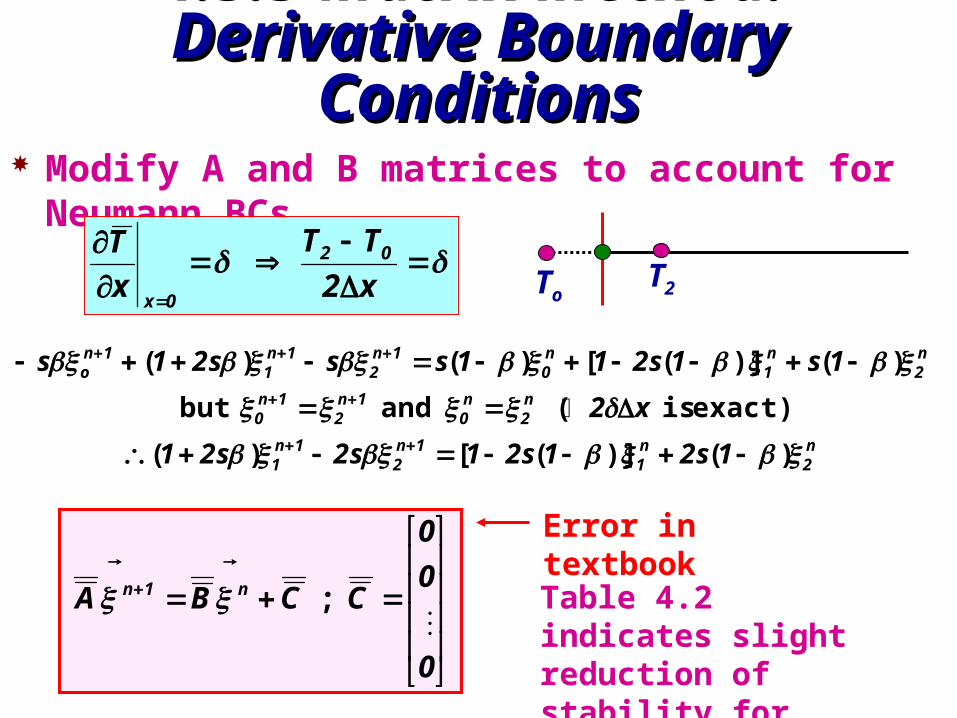
4.3.3 Matrix Method: 4.3.3 Matrix Method: Derivative Boundary ConditionsDerivative Boundary Conditions
Modify A and B matrices to account for Neumann BCs
x2
TT
x
T 02
0x
To
T2
n2
n1
1n2
1n1
n2
n0
1n2
1n0
n2
n1
n0
1n2
1n1
1no
1s21s21s2s21
x2
1s1s211sss21s
)()]([)(
exact) is ( and but
)()]([)()(
;
0
0
0
CCBA n1n
Table 4.2 indicates slight
reduction of stability for Neumann conditions
Error in textbook
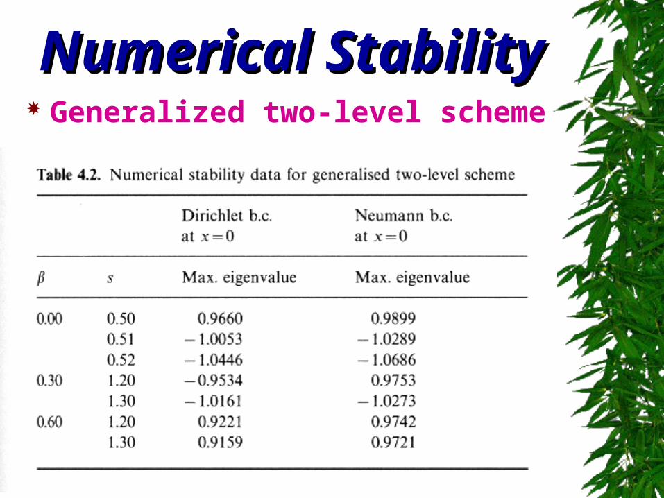
Numerical StabilityNumerical Stability Generalized two-level scheme
Von Neumann MethodVon Neumann Method Fourier stability method
Most commonly used, easy to apply, straightforward and dependable
Can only be used for linear, initial value problem (propagation problem) with constant coefficients
for nonlinear problems with variable coefficients, the method may still be applied “locally” to provide necessary, but not sufficient stability criterion
may also provide heuristic information about the influence at the boundary
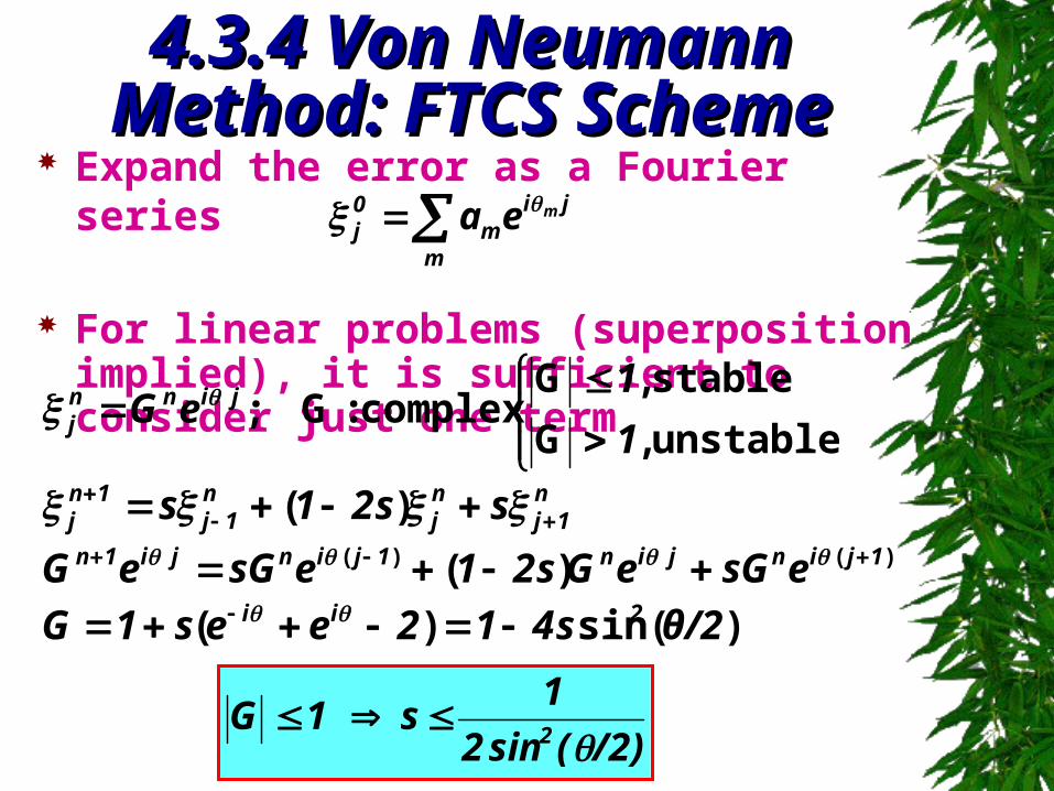
4.3.4 Von Neumann Method: 4.3.4 Von Neumann Method: FTCS SchemeFTCS Scheme
Expand the error as a Fourier series
For linear problems (superposition implied), it is sufficient to consider just one term
ji
mm
0j
mea
)(sin)(
)(
)(
unstable ,G
stable ,Gcomplex :G ;
)( )(
2θ/s412ees1G
esGeGs21esGeG
ss21s
1
1eG
2ii
1jinjin1jinji1n
n1j
nj
n1j
1nj
jinnj
)/2(sin2
1s 1G
2
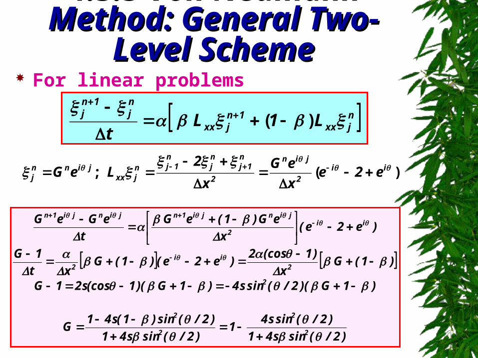
4.3.5 Von Neumann Method: 4.3.5 Von Neumann Method: General Two-Level SchemeGeneral Two-Level Scheme
For linear problems
)( ;
ii
2
jin
2
n1j
nj
n1jn
jxxjinn
j e2ex
eG
x
2 LeG
)( njxx
1njxx
nj
1nj L1L
t
)2/(sins41
)2/(sins41
)2/(sins41
)2/(sin)1(s41G
)1G )(2/(sins4)1G )(1(coss21G
)1(G x
)1(cos2)e2e()1(G
xt
1G
)e2e(x
eG )1(eG
t
eGeG
2
2
2
2
2
2ii
2
ii2
j inj i1nj inj i1n
Von Neumann MethodVon Neumann Method For more complex equations, it may be necessary
to evaluate the amplification factor G(s,, ) numerically for a range of s,, and values
For three time level schemes, need to solve a quadratic equation in G
For a system of equations of several variables (i.e., u, v, w, p), need to solve the eigenvalues for amplification matrix and require |m| 1
This section deals with numerical instability, but not the physical instability (transition to turbulence)
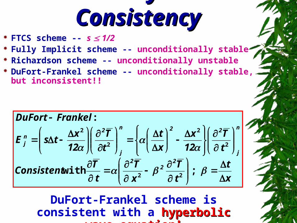
Stability and ConsistencyStability and Consistency FTCS scheme -- s 1/2 Fully Implicit scheme -- unconditionally stable Richardson scheme -- unconditionally unstable DuFort-Frankel scheme -- unconditionally stable, but
inconsistent!!
x
t
t
T
x
T
t
TConsistent
t
T
12
x
x
t
t
T
12
xtsE
FrankelDuFort
22
2
n
j
22n
j
2nj
;
with
:
22
2
2
2
2
DuFort-Frankel scheme is consistent with a hyperbolic wave equation!hyperbolic wave equation!
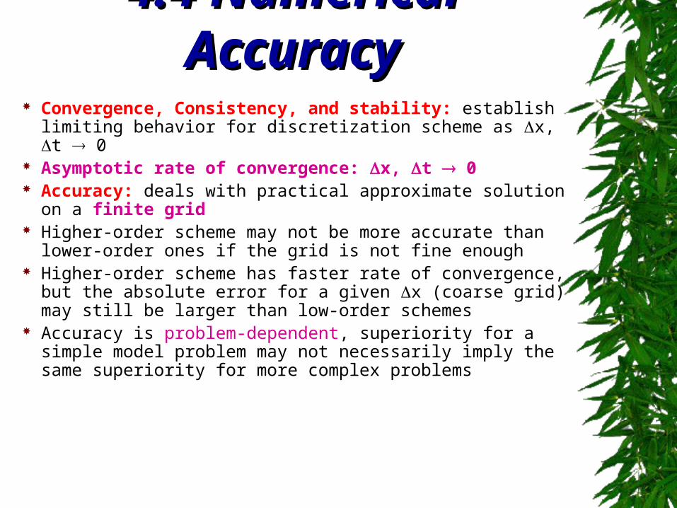
4.4 Numerical Accuracy4.4 Numerical Accuracy Convergence, Consistency, and stability: establish limiting
behavior for discretization scheme as x, t 0 Asymptotic rate of convergence: x, t 0 Accuracy: deals with practical approximate solution on a finite
grid Higher-order scheme may not be more accurate than lower-
order ones if the grid is not fine enough Higher-order scheme has faster rate of convergence, but the
absolute error for a given x (coarse grid) may still be larger than low-order schemes
Accuracy is problem-dependent, superiority for a simple model problem may not necessarily imply the same superiority for more complex problems
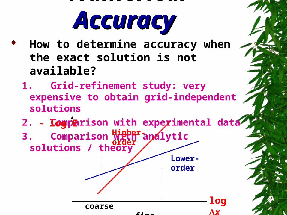
Numerical AccuracyNumerical Accuracy How to determine accuracy when the exact
solution is not available? 1. Grid-refinement study: very expensive to obtain
grid-independent solutions
2. Comparison with experimental data
3. Comparison with analytic solutions / theory
Lower-order
Higher-order
coarse finelog x
log E
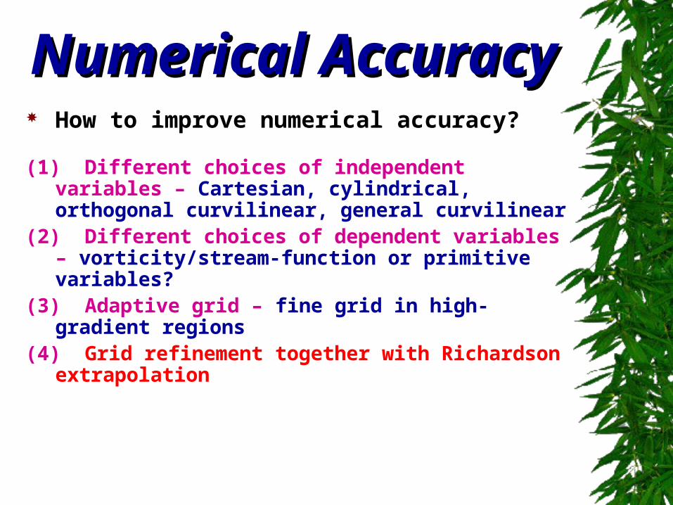
Numerical AccuracyNumerical Accuracy How to improve numerical accuracy?
(1) Different choices of independent variables – Cartesian, cylindrical, orthogonal curvilinear, general curvilinear
(2) Different choices of dependent variables – vorticity/stream-function or primitive variables?
(3) Adaptive grid – fine grid in high-gradient regions(4) Grid refinement together with Richardson
extrapolation
4.4.1 Richardson Extrapolation 4.4.1 Richardson Extrapolation Numerical accuracy may be established through
successive grid refinements For a sufficiently fine grid, the solution error reduces like
the leading term of truncation error
Richardson extrapolation: cancel the leading term of truncation error for two numerical solutions with different grid resolutions to achieve higher-order accuracy
Assume that the leading term dominate the truncation error, valid only if x is sufficiently fine
More economical than using higher-order scheme directly
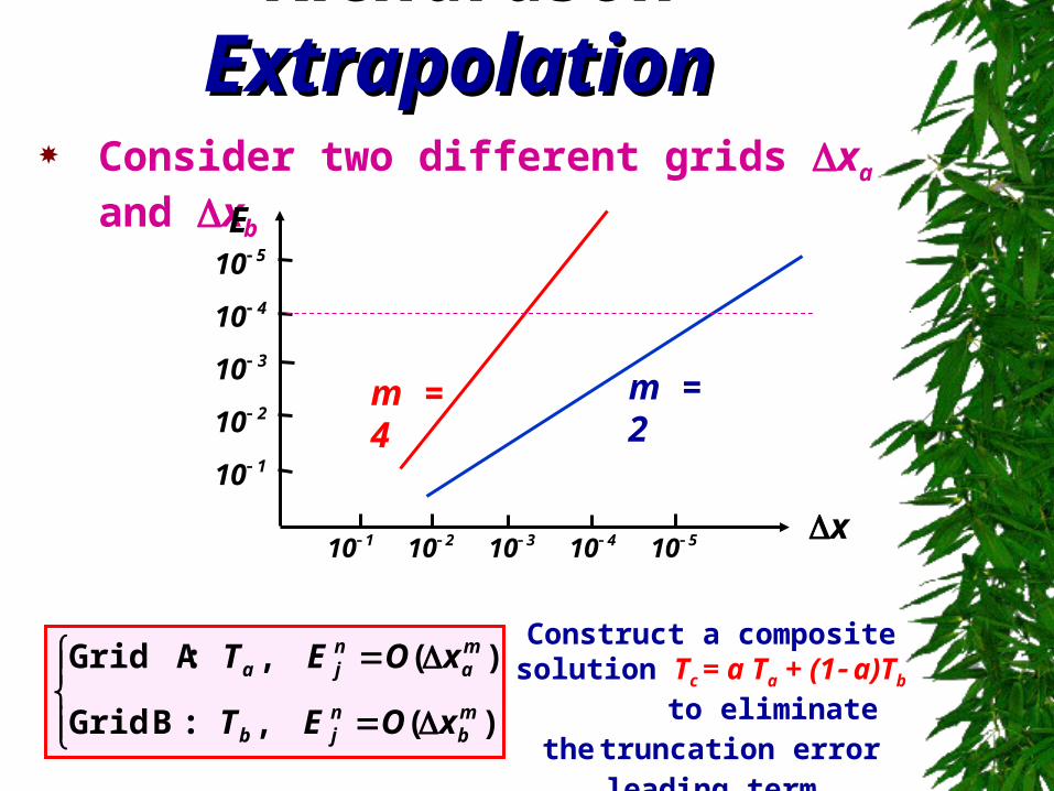
Richardson ExtrapolationRichardson Extrapolation Consider two different grids xa and xb
m = 2m = 4
54321 1010101010
1
2
3
4
5
10
10
10
10
10
)( , :B Grid
)( , : AGrid
mb
njb
ma
nja
xOET
xOETConstruct a composite solution Tc = a Ta + (1 a)Tb to eliminate the truncation error
leading term
x
E
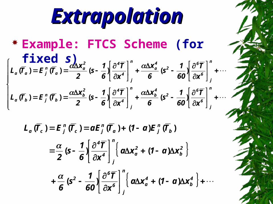
Richardson ExtrapolationRichardson Extrapolation Example: FTCS Scheme (for fixed s)
n
j6
62
4b
n
j4
42b
bnjba
n
j6
62
4a
n
j4
42a
anjaa
x
T
60
1s
6
x
x
T
6
1s
2
xTETL
x
T
60
1s
6
x
x
T
6
1s
2
xTETL
)()()()(
)()()()(
)( )(
)( )(
)()()()()(
4b
4a
n
j6
62
2b
2a
n
j4
4
bnja
njc
njca
xa1xax
T
60
1s
6
xa1xax
T
6
1s
2
TEa1TaETETL
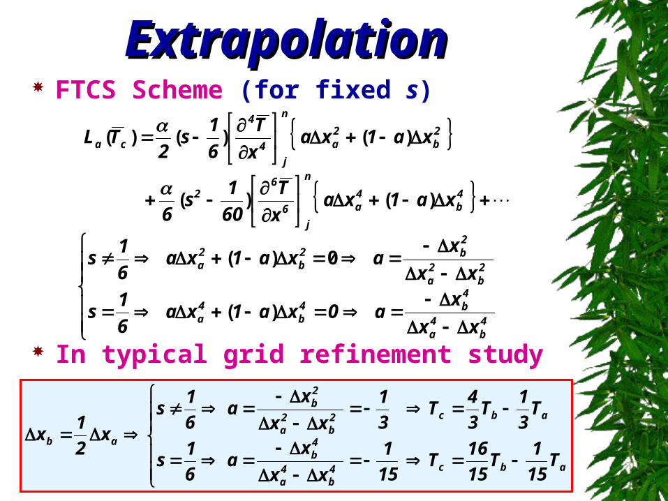
Richardson ExtrapolationRichardson Extrapolation FTCS Scheme (for fixed s)
In typical grid refinement study
)( )(
)( )()(
4b
4a
n
j6
62
2b
2a
n
j4
4
ca
xa1xax
T
60
1s
6
xa1xax
T
6
1s
2TL
)(
0 )(
4b
4a
4b4
b4a
2b
2a
2b2
b2a
xx
xa0xa1xa
6
1s
xx
xaxa1xa
6
1s
abc4b
4a
4b
abc2b
2a
2b
ab
T15
1T
15
16T
15
1
xx
xa
6
1s
T3
1T
3
4T
3
1
xx
xa
6
1s
x2
1x
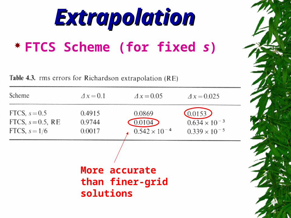
Richardson ExtrapolationRichardson Extrapolation FTCS Scheme (for fixed s)
More accurate than finer-grid solutions