Embed Size (px)
Citation preview

Chapter 4Chapter 4
Using Probability and Using Probability and Discrete Probability Discrete Probability
DistributionsDistributions
©

Chapter 4 - Chapter 4 - Chapter Chapter OutcomesOutcomes
After studying the material in this chapter, you should be able to:
• Understand the three approaches to assessing probabilities.
• Apply the common rules of probability.
• Identify the types of processes that are represented by discrete probability distributions.

Chapter 4 - Chapter 4 - Chapter Chapter OutcomesOutcomes
(continued)(continued)
After studying the material in this chapter, you should be able to:
• Know how to determine probabilities associated with binomial and Poisson distribution applications.

ProbabilityProbability
ProbabilityProbability refers to the chance refers to the chance that a particular event will that a particular event will
occur.occur.•The probability of an event will be a value in the range 0.00 to 1.00. A value of 0.00 means the event will not occur. A probability of 1.00 means the event will occur. Anything between 0.00 and 1.00 reflects the uncertainty of the event occurring.
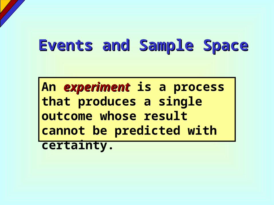
Events and Sample SpaceEvents and Sample Space
An experimentexperiment is a process that produces a single outcome whose result cannot be predicted with certainty.

Events and Sample SpaceEvents and Sample Space
Elementary eventsElementary events are the most rudimentary outcomes resulting from a simple experiment.

Events and Sample SpaceEvents and Sample Space
The sample spacesample space is the collection of all elementary outcomes that can result from a selection or decision.

Events and Sample SpaceEvents and Sample Space
An eventevent is a collection of elementary events.
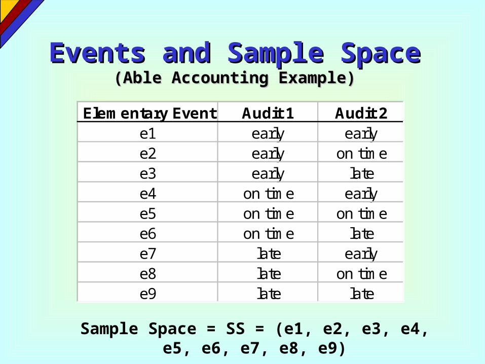
Elementary Event Audit 1 Audit 2e1 early earlye2 early on timee3 early latee4 on time earlye5 on time on timee6 on time latee7 late earlye8 late on timee9 late late
Events and Sample SpaceEvents and Sample Space(Able Accounting Example)(Able Accounting Example)
Sample Space = SS = (e1, e2, e3, e4, e5, e6, e7, e8, e9)

Mutually Exclusive EventsMutually Exclusive Events
Two events are mutually mutually exclusiveexclusive if the occurrence of one event precludes the occurrence of a second event.
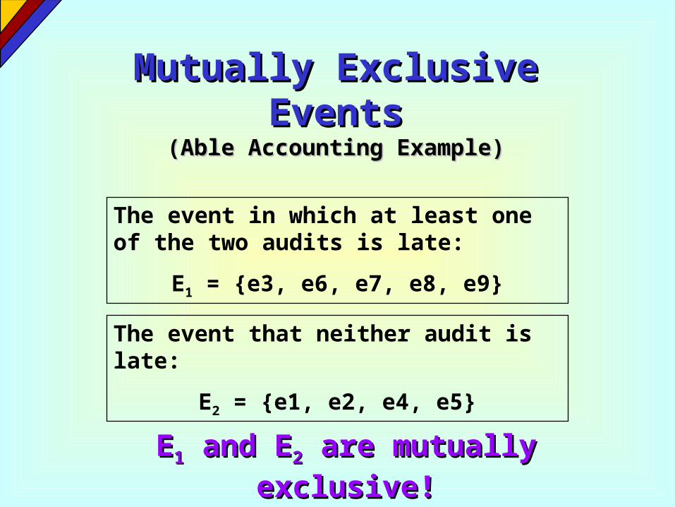
Mutually Exclusive EventsMutually Exclusive Events(Able Accounting Example)(Able Accounting Example)
The event in which at least one of the two audits is late:
E1 = {e3, e6, e7, e8, e9}
The event that neither audit is late:
E2 = {e1, e2, e4, e5}
EE11 and E and E22 are mutually are mutually exclusive!exclusive!

Independent and Independent and Dependent EventsDependent Events
Two events are independent independent if the occurrence of one event in no way influences the probability of the occurrence of the other event.

Independent and Independent and Dependent EventsDependent Events
Two events are dependent dependent if the occurrence of one event impacts the probability of the other event occurring.

Classical Probability Classical Probability AssessmentAssessment
Classical Probability AssessmentClassical Probability Assessment refers to the method of determining probability based on the ratio of the number of ways the event of interest can occur to the total number of ways any event can occur when the individual elementary events are equally likely.

CLASSICAL PROBABILITY MEASUREMENTCLASSICAL PROBABILITY MEASUREMENT
Classical Probability Classical Probability AssessmentAssessment
events elementaryof number Totaloccur can E of ways Number
P(E ii )
Relative Frequency of Relative Frequency of OccurrenceOccurrence
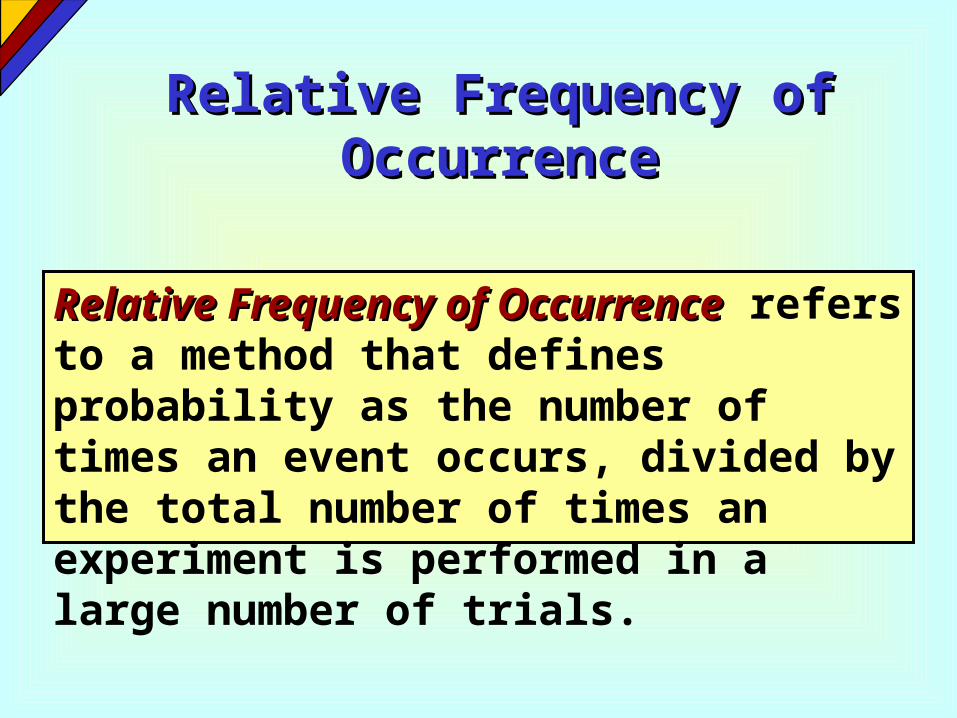
Relative Frequency of OccurrenceRelative Frequency of Occurrence refers to a method that defines probability as the number of times an event occurs, divided by the total number of times an experiment is performed in a large number of trials.
Relative Frequency of Relative Frequency of OccurrenceOccurrence
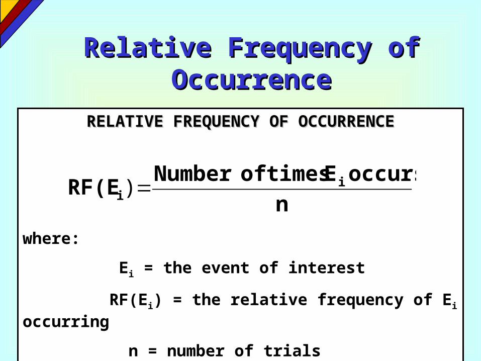
RELATIVE FREQUENCY OF OCCURRENCERELATIVE FREQUENCY OF OCCURRENCE
where:
Ei = the event of interest
RF(Ei) = the relative frequency of Ei occurring
n = number of trials
noccurs E timesof Number
RF(E ii )

Relative Frequency of Relative Frequency of OccurrenceOccurrence
(Example 4-6)(Example 4-6)
Commercial Residential TotalHeating Systems 55 145 200Air-ConditioningSystems 45 255 300Total 100 400 500
80.0500
400)(Re)(Re sidentialRFsidentialP
40.0500
200)()( HeatingRFHeatingP

Subjective Probability Subjective Probability AssessmentAssessment
Subjective Probability Subjective Probability AssessmentAssessment refers to the method that defines probability of an event as reflecting a decision maker’s state of mind regarding the chances that the particular event will occur.

The Rules of ProbabilityThe Rules of Probability
PROBABILITY RULE 1PROBABILITY RULE 1
For any event Ei
0.0 P(Ei) 1.0 for all i

The Rules of ProbabilityThe Rules of Probability
PROBABILITY RULE 2PROBABILITY RULE 2
where:k = Number of elementary
events in the sample space
ei = ith elementary event
0.1)(1
k
iieP

The Rules of ProbabilityThe Rules of Probability
PROBABILITY RULE 3PROBABILITY RULE 3The probability of an event Ei is equal to the sum of the probabilities of the elementary events forming Ei. That is, if:
Ei = {e1, e2, e3}
then:
P(Ei) = P(e1) + P(e2) + P(e3)

ComplementsComplements
The complement complement of an event E is the collection of all possible elementary events not contained in event E. The complement of event E is represented by E.

The Rules of ProbabilityThe Rules of Probability
COMPLEMENT RULECOMPLEMENT RULE
)(1)( EPEP

The Rules of ProbabilityThe Rules of Probability
PROBABILITY RULE 4PROBABILITY RULE 4
Addition rule for any two events E1 and E2:
P(E1 or E2) = P(E1) + P(E2) - P(E1 and E2)

The Rules of ProbabilityThe Rules of Probability
PROBABILITY RULE 5PROBABILITY RULE 5
Addition rule for mutually exclusive events E1 and E2:
P(E1 or E2) = P(E1) + P(E2)

Conditional ProbabilityConditional Probability
Conditional probabilityConditional probability refers to the probability that an event will occur given that some other event has already happened.
The Rules of ProbabilityThe Rules of Probability
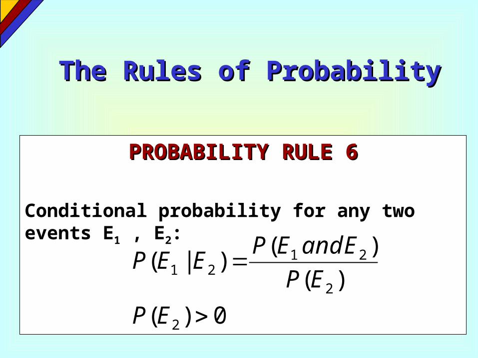
PROBABILITY RULE 6PROBABILITY RULE 6
Conditional probability for any two events E1 , E2:
0)(
)(
)()|(
2
2
2121
EP
EP
EandEPEEP

Tree DiagramsTree Diagrams
Another way of organizing events of an experiment that aids in the calculation of probabilities is the tree tree diagramdiagram.

Tree DiagramsTree Diagrams(Figure 4-1)(Figure 4-1)
Female P(E4) =
0.34
Male P(E5) =
0.66

Tree DiagramsTree Diagrams (Figure 4-1)(Figure 4-1)
Female P(E4) =
0.34
Male P(E5) =
0.66
P(E1) = 0.38 P(E2) =
0.44
P(E3) = 0.18
P(E1) = 0.38 P(E2) =
0.44
P(E3) = 0.18

Tree DiagramsTree Diagrams (Figure 4-1)(Figure 4-1)
Female P(E4) =
0.34
Male P(E5) =
0.66
P(E1) = 0.38 P(E2) =
0.44
P(E3) = 0.18
P(E1) = 0.38 P(E2) =
0.44
P(E3) = 0.18
P(E1 and E5) = 0.38 x 0.66 = 0.20
P(E2 and E5) = 0.44 x 0.66 = 0.32
P(E3 and E5) = 0.18 x 0.66 = 0.14
P(E1 and E4) = 0.38 x 0.34 = 0.18 P(E2 and E4) = 0.44 x 0.34 = 0.12
P(E3 and E4) = 0.18 x 0.34 = 0.04

The Rules of ProbabilityThe Rules of Probability
PROBABILITY RULE 7PROBABILITY RULE 7
Conditional probability for independent events E1 , E2:
0)();()|(
0)();()|(
1212
2121
EPEPEEP
and
EPEPEEP

The Rules of ProbabilityThe Rules of Probability
PROBABILITY RULE 8PROBABILITY RULE 8
Multiplication rule two events E1 and E2:
)|()()(
)|()()(
21212
12121
EEPEPEandEP
and
EEPEPEandEP

The Rules of ProbabilityThe Rules of Probability
PROBABILITY RULE 9PROBABILITY RULE 9
Multiplication rule independent events E1 , E2:
)()()( 2121 EPEPEandEP

Bayes’ TheoremBayes’ Theorem
BAYES’ THEOREMBAYES’ THEOREM
where:Ei = ith event of interest of the k
possible eventsB = new event that might impact
P(Ei)
)|()()|()()|()(
)|()()|(
2211 kk
iii EBPEPEBPEPEBPEP
EBPEPBEP

Discrete Probability Discrete Probability DistributionsDistributions
A random variablerandom variable is a variable that assigns a numerical value to each outcome of a random experiment or trial.

Discrete Probability Discrete Probability DistributionsDistributions
A discrete random discrete random variablevariable is a variable that can only assume a countable number of values.

Discrete Probability Discrete Probability DistributionsDistributions
A continuous random variablecontinuous random variable is a variable that can assume any value on a continuum. Alternatively, they are random variables that can assume an uncountable number of values.
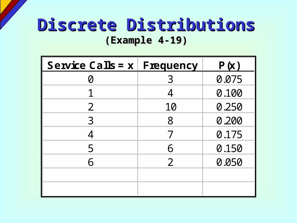
Discrete DistributionsDiscrete Distributions(Example 4-19)(Example 4-19)
Service Calls = x Frequency P(x)0 3 0.0751 4 0.1002 10 0.2503 8 0.2004 7 0.1755 6 0.1506 2 0.050
1 0 00.

Discrete DistributionsDiscrete Distributions(Example 4-19)(Example 4-19)
Discrete Probability Distribution
x = Number of service calls
0.000
0.050
0.100
0.150
0.200
0.250
0.300
0 1 2 3 4 5 6

Discrete Probability Discrete Probability DistributionsDistributions
The uniform probability uniform probability distributiondistribution is a probability distribution that has equal probabilities for all possible outcomes of the random variable

Discrete DistributionsDiscrete Distributions(Example 4-20)(Example 4-20)
Uniform Probability Distribution
Delivery Lead Time
0
0.05
0.1
0.15
0.2
0.25
0.3
1 week 2 weeks 3 weeks 4 weeks

Mean and Standard Mean and Standard Deviation of Discrete Deviation of Discrete
DistributionsDistributions
EXPECTED VALUE FOR A DISCRETE EXPECTED VALUE FOR A DISCRETE DISTRIBUTIONDISTRIBUTION
where:E(x) = Expected value of the random
variable x = Values of the random variableP(x) = Probability of the random variable
taking on the value of x
)()( xxPxE

Mean and Standard Mean and Standard Deviation of Discrete Deviation of Discrete
DistributionsDistributions
STANDARD DEVIATION FOR A DISCRETE STANDARD DEVIATION FOR A DISCRETE DISTRIBUTIONDISTRIBUTION
where:E(x) = Expected value of the random
variable x = Values of the random variableP(x) = Probability of the random variable
having the value of x
)()}({ xPxEx 2x

Binomial Probability Binomial Probability DistributionDistribution
• A manufacturing plant labels items as either defective or acceptable.
• A firm bidding for a contract will either get the contract or not.
• A marketing research firm receives survey responses of “Yes, I will buy,” or “No, I will not.”
• New job applicants either accept the offer or reject it.

Binomial Probability Binomial Probability DistributionDistribution
Characteristics of the Binomial Characteristics of the Binomial Probability Distribution:Probability Distribution:
• A trial has only two possible outcomes – a success or a failure.
• There is a fixed number, n, of identical trials.• The trials of the experiment are independent
of each other and randomly generated.• The probability of a success, p, remains
constant from trial to trial.• If p represents the probability of a success,
then (1-p) = q is the probability of a failure.

CombinationsCombinations
A combinationcombination is an outcome of an experiment where x objects are selected from a group of n objects.

CombinationsCombinations
COUNTING RULE FOR COMBINATIONSCOUNTING RULE FOR COMBINATIONS
where:n! =n(n - 1)(n - 2) . . . (2)(1)
x! = x(x - 1)(x - 2) . . . (2)(1) 0! = 1
)!(!
!
xnx
nC nx

Binomial Probability Binomial Probability DistributionDistribution
BINOMIAL FORMULABINOMIAL FORMULA
where:
n = sample size
x = number of successes n - x = number of failures
p = probability of a successq = 1 - p = probability of a failuren! =n(n - 1)(n - 2) . . . (2)(1)
x! = x(x - 1)(x - 2) . . . (2)(1) 0! = 1
xnxqpxnx
nxP
)!(!
!)(
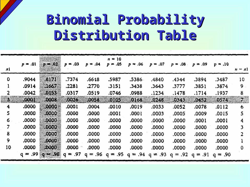
Binomial Probability Binomial Probability Distribution TableDistribution Table
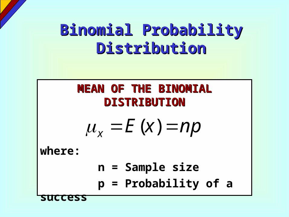
Binomial Probability Binomial Probability DistributionDistribution
MEAN OF THE BINOMIAL MEAN OF THE BINOMIAL DISTRIBUTIONDISTRIBUTION
where:n = Sample sizep = Probability of a
success
npxEx )(

Binomial Probability Binomial Probability DistributionDistribution
STANDARD DEVIATION FOR THE STANDARD DEVIATION FOR THE BINOMIAL DISTRIBUTIONBINOMIAL DISTRIBUTION
where:n = Sample sizep = Probability of a successq = (1 - p) = Probability of a
failure
npq

Poisson Probability Poisson Probability DistributionDistribution
Characteristics of the Poisson Characteristics of the Poisson Probability Distribution:Probability Distribution:
• The outcomes of interest are rare relative to the possible outcomes.
• The average number of outcomes of interest per segment is ..
• The number of outcomes of interest are random, and the occurrence of one outcome does not influence the chances of another outcome of interest.
• The probability of that an outcome of interest occurs in a given segment is the same for all segments.

Poisson Probability Poisson Probability DistributionDistribution
POISSON PROBABILITY DISTRIBUTIONPOISSON PROBABILITY DISTRIBUTION
where:
x = number of successes in segment t
t = expected number of successes in segment te =base of the natural number system (2.71828)
!
)()(
x
etxP
tx

Poisson Probability Poisson Probability Distribution TableDistribution Table
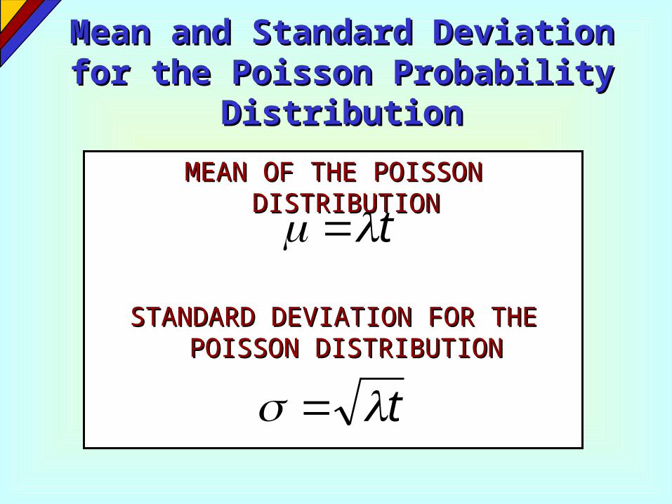
Mean and Standard Mean and Standard Deviation for the Poisson Deviation for the Poisson Probability DistributionProbability Distribution
MEAN OF THE POISSON MEAN OF THE POISSON DISTRIBUTIONDISTRIBUTION
STANDARD DEVIATION FOR THE STANDARD DEVIATION FOR THE POISSON DISTRIBUTIONPOISSON DISTRIBUTION
t
t

Key TermsKey Terms
• Binomial Probability Distribution
• Classical Probability• Conditional
Probability• Continuous Random
Variable• Dependent Events• Discrete Random
Variable
• Elementary Events• Event• Independent Events• Mutually Exclusive
Events• Poisson Probability
Distribution• Probability• Random Variable

Key TermsKey Terms(continued)(continued)
• Relative Frequency of Occurrence
• Sample Space• Subjective Probability
Assessment• Uniform Probability
Distribution