Chapter 5 Case Study – Merlinleigh Sub-basin, Western ... · a magnetic basement high (labelled B in Figure 5.2). Iasky et al. (1998) have also divided the magnetic basement into

Chapter 5 - Case Study – Merlinleigh Sub-basin, Western Australia

151

Chapter 5 Case Study – Merlinleigh Sub-basin, Western Australia

5.1 Introduction

The previous three chapters of this thesis have described geometric, stochastic and spectral

methods of estimating fractal dimension (FD) and tested these methods on a variety of

synthetic datasets. These synthetic datasets were intentionally designed to be simplistic in

order to investigate how FD estimation techniques work and what potential these techniques

have for enhancing aeromagnetic data. However, in order for these methods to have a

demonstrable role in interpreting aeromagnetic data they must be shown to effectively

enhance real aeromagnetic data. Consequently, this Chapter investigates the effectiveness of

the FD estimation techniques on an airborne magnetic dataset from the Merlinleigh Sub-

basin, Western Australia.

This Chapter aims to answer three questions.

1. Which of the FD estimation techniques effectively enhance the airborne magnetic data

from the Merlinleigh Sub-basin?

2. What are the key differences and similarities between the various FD estimation

techniques?

3. Are there significant differences between the results from the 1D and 2D methods of

estimating FD?

The ideal approach to answering these questions would be to apply the FD estimation

techniques to a dataset and then compare the results with something that is previously

constrained by comprehensively defined geology. Unfortunately, airborne magnetic data are

rarely obtained in regions where the geology is totally constrained. Consequently, this thesis

takes the approach of comparing the FD estimation methods with other conventional and

widely accepted enhancements. Whilst numerous enhancements exist to aid in the

interpretation of aeromagnetic data, three of the most common enhancements are considered

here, specifically:

� a vertical derivative;

� a total horizontal derivative;


152

� an analytic signal, and;

� automatic gain control (AGC).

These specific enhancements are all designed to enhance high-wavenumber features and

hence should enhance similar features to the FD estimators.

It should be emphasised that the aim of this Chapter is not to provide a detailed structural

interpretation of the Merlinleigh Sub-basin. Rather, the aim is to compare the various

methods of FD estimation with conventional enhancement techniques and to investigate what

use they could be in interpreting airborne magnetic data similar to the Merlinleigh dataset.

5.2 Setting

5.2.1 Geology and Structural Evolution of the Merlinleigh Sub-basin

The Merlinleigh Sub-basin is part of the onshore Carnarvon basin in north-west Western

Australia (Figure 5.1). The region’s Precambrian basement is overlain by a sedimentary

succession up to 8 000 m thick. This succession contains sandstones, siltstones, carbonates

and limestones varying in age from Ordovician1 to Permian. In addition to this succession,

the region has some thin (i.e. less than 100 m) Cretaceous shales, sandstones and siltstones, as

well as a veneer of Tertiary sediments.

The Merlinleigh Sub-basin has been subjected to three significant periods of tectonic activity

which are responsible for the structures observed in the region. The first of these was a period

of rifting that extended throughout the Merlinleigh Sub-basin and Perth Basin from the Late

Carboniferous till the Early Permian. This period of rifting is believed to have created a series

of northerly trending en echelon fault systems in the Merlinleigh Sub-basin, specifically the

Kennedy and Wandagee systems. These rift fault systems formed during a period of

ENE-WSW extension. However, the presence of en echelon faults suggests that some soft-

linked strike-slip movement occurred (O'Brien et al., 1996).

1 According to Iasky et al. (1998), there is some debate over the age of the region’s oldest unit, the Tumblagooda

Sandstone, with possible ages ranging from Silurian to Cambro-Ordivician. The unit is simply referred to as

Ordivician for convenience in this thesis.


153

Figure 5.1: Location of the Merlinleigh Sub-basin Aeromagnetic Survey

The next significant tectonic event was the break-up of Australia and Greater India during the

Early Cretaceous. This break-up led to a transtensional stress field across the Merlinleigh

Sub-basin, with the principal axis of extension oriented NW-SE (Dentith et al., 1993). This

stress field reactived major north-trending faults in the region and led to the creation of a

series of north-west-trending transfer faults west of the region (Iasky et al., 1998). A series of

north-trending anticlines are also attributed to this period of tectonism.

Following this break-up, the convergence of the Australian and Eurasian Plates during the

Miocene led to a compressional stress field across the Australian Plate. The principle axis of

compression across the Merlinleigh Sub-basin was oriented north-south and led to the

reactivation of faults in the region. Specifically, the Miocene tectonism led to strike-slip

movement along north-easterly oriented faults. It also led to significant normal movement

along north trending faults within the region (Iasky et al., 1998).


154

5.2.2 Data Description and Processing

The aeromagnetic dataset examined in this Chapter was acquired by the Geological Survey of

Western Australia (GSWA) to aid petroleum exploration in the region. The dataset was

acquired to allow structural interpretations to be carried out in regions where little or no data

had previously existed. This interpretation attempted to infer or extrapolate trends seen in

nearby seismic data and outcrop into previously unexplored parts of the Merlinleigh

Sub-basin.

The dataset consists of 45 305 line-km of data acquired by Tesla Airborne Geoscience for the

GSWA in 1995. The survey was flown using a traverse-line spacing of 500 m at an

orientation of 067� N. Tie-lines were flown perpendicular to the traverse-lines with a spacing

of 1 500 m. Samples were taken approximately every 7.5 m with a sensitivity of 0.01 nT.

Pre-processed grids of reduced to pole (RTP) total magnetic intensity (TMI) data have been

provided by the GSWA, and are presented in the following section. The datasets were tie-line

levelled, microlevelled and then gridded using a 125 m grid cell size. The gridding was

carried out using Tesla Airborne Geoscience’s in house linear tensioned spline algorithm.

For comparison, Table 5-1 provides a summary of the FD methods processing time for this

dataset. It is clear from this table that the 2D methods are significantly faster than their 1D

equivalents.

1D 2D

Variation 116 mins 4 mins

Semi-variogram 73 mins 4 mins

Hurst na 7 mins

Gabor 24 mins 6 mins

Wavelet 16 mins 7 mins

Table 5-1: Processing times for the FD methods on the Merlinleigh data.


155

5.3 Results

5.3.1 Conventional Enhancement

The airborne magnetic data considered in this section have been previously interpreted by

Iasky et al. (1998). This interpretation was based primarily on two conventional

enhancements, specifically a colourdraped image of the RTP-TMI (Figure 5.2)1 and the

vertical derivative of the RTP-TMI (Figure 5.3). Iasky et al. (1998) commented that the

region has a relatively low magnetic signature, and a brief examination of Figure 5.2 suggests

that the TMI in the region is generally smooth. The data have been interpreted as a series of

anomalies associated with basement features, faults, outcrops or localised near-surface

features.

The basement features interpreted by Iasky et al. (1998) are most easily seen on the RTP-TMI

image (Figure 5.2). The regions of lowest magnetic intensity generally correspond to areas

with the deepest burial of magnetic basement. However, a low-wavenumber magnetic high in

an area of thick sediment cover (labelled A in Figure 5.2) suggests a magnetic body at depth

in this region. In contrast, there is another low-wavenumber magnetic high that corresponds to

a magnetic basement high (labelled B in Figure 5.2). Iasky et al. (1998) have also divided the

magnetic basement into three regions of differing fabric by two north-trending lineaments

(white lines on Figure 5.2).

The magnetic basement high in the eastern margin of the RTP-TMI image is cross-cut by a

series of west and north-west-trending lineaments (labelled B in Figure 5.2). Iasky et al.

(1998) attribute these lineaments to structures limited to the shallow or outcropping magnetic

basement. The cross-cutting lineaments are not seen in regions where the magnetic basement

is under significant cover which suggests that they are shallow features.

1 All of the figures within Section 5.3 have been placed at the end of the Section in order to allow for easy

comparison of the various enhancements.


156

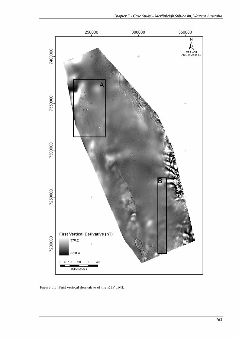
Figure 5.3 presents the first vertical derivative of the RTP-TMI data which highlights some of

the high-wavenumber features interpreted by Iasky et al. (1998). The first clearly identifiable

feature is a series of high-wavenumber, high-amplitude anomalies in the north-west of the

image (labelled A in Figure 5.3) which can be attributed to previously mapped kimberlites

(Atkinson et al., 1984; Jaques et al., 1986). A subtle, north-trending lineament in the south-

east of the image is associated with the Dampier-Pinjarra gas pipeline (labelled B in Figure

5.3).

The western margin of the image has a series of north-trending lineaments which are

associated with Wandagee fault (labelled A in Figure 5.3). This fault is not seen as a single

lineament, but rather as a series of discontinuous high-wavenumber features that are thought

to be associated with a deep intrusive body (Iasky et al., 1998). In addition to these clear high-

wavenumber anomalies, Iasky et al. (1998) identify numerous subtler NNW-trending

lineaments throughout the study region. These lineaments are thought to be due to surface

mineralisation of sand dunes and outcropping basement.

An image of the total horizontal derivative of the RTP TMI is presented in Figure 5.4. This

image appears to be very similar to the vertical derivative image presented in Figure 5.3. The

kimberlites to the north-west of the image are clearly visible in this image (labelled A in

Figure 5.4). Similarly, the gas pipeline to the south-east of the image is again clearly

enhanced (labelled B in Figure 5.4).

The analytic signal of the RTP TMI (Figure 5.5) enhances the same features as the vertical

and total horizontal derivatives (Figures 5.3-5.4). For example, both the kimberlites in the

north-west and the gas pipeline in the south-east are clearly enhanced in this image (labelled

A and B in Figure 5.5).

Automatic gain control using a 7x7 point window has been applied to the RTP TMI (Figure

5.6). The resultant image tends to enhance the shallow, high-wavenumber features within the

dataset, especially the kimberlites in the north-west (labelled A in Figure 5.6) and the shallow

and outcropping magnetic basement in the east (labelled B in Figure 5.6). In addition to these

features, there is a region of highly variable data in the central part of the image (labelled C in

Figure 5.6). These highly variable data are not discussed specifically by Iasky et al. (1998),

however the region has a general strike similar to the lineaments attributed to surface

mineralisation of sand dunes and outcropping basement.


157

5.3.2 Geometric FD Enhancement

The 1D and 2D variation methods have been applied to the aeromagnetic data from the

Merlinleigh Sub-basin, based on the results of Chapter 2. The 2D variation method was

applied to the RTP-TMI data presented in Section 5.3.1. The 1D variation method was

applied to the microlevelled TMI data, and then gridded using INTREPID 5.3’s tensioned

spline algorithm with a 125 m cell size. The optimum window size for both of the methods

was selected by trying a suite of window sizes and visually inspecting the results to determine

which window size provides the clearest enhancement of key structural features. In the case

of the 1D method, a window size of 31 data points was found to give the best results for this

dataset. A window size of 7x7 points provided the best results for the 2D variation method.

The result of applying the 2D variation method is presented in Figure 5.7. A superficial

inspection of Figure 5.7 suggests that the 2D variation method enhances more high-

wavenumber information than the conventional enhancements described in Section 5.3.1, with

the exception of the AGC which appears to have more high-wavenumber content. Both the

kimberlites in the north-west (labelled A in Figure 5.7) and the Dampier-Pinjarra gas pipeline

in the south-east (labelled B in Figure 5.7) are enhanced in this image. Furthermore, both

these features are associated with large amplitude FD anomalies making them very easy to

detect.

The region of shallow and outcropping magnetic bedrock to the east of the region (labelled D

in Figure 5.7) is also enhanced in this image. The main features that are strongly enhanced

are the shallow west and north-west-trending lineaments that cross cut the magnetic bedrock

(labelled D in Figure 5.7).

Figure 5.7 also exhibits regions of generally high FD such as in the region labelled C. This

area corresponds to the area of highly variable data enhanced in the AGC image (Labelled C

in Figure 5.6). Unlike in the AGC image, there are no defined trends within this region in the

2D variation method image. In contrast, the region appears to contain ‘smeared’ high FD that

does not clearly delineate any high-wavenumber features. This suggests that the data are so

variable within this region that the moving window approach used by the 2D variation method

is unable to differentiate between individual peaks and troughs. Consequently, the region is

seen as being generally rough and hence having a high FD.


158

The results of the 1D variation method are presented in Figure 5.8. A superficial inspection

of Figure 5.8 suggests that the 1D variation method is not as suited to this style of data as the

2D variation method. The image is dominated by broad regions of ‘smeared’ high FD, and

the previously identified high-wavenumber features are very difficult to observe in the data.

For example, the kimberlites in the north-west of the study area are generally undetectable in

the area labelled A in Figure 5.8. The Dampier-Pinjarra gas pipeline can be seen in the south-

east of the image, however it is neither as extensive nor as easily detectable as on other

enhancements such as the 2D variation method (labelled B in Figure 5.8).

The 1D variation method has also enhanced a series of ridges or corrugations that parallel the

flight line direction. This study region is known to be of difficult terrain, and the dataset had

been significantly microlevelled prior to processing. However, despite this miocrolevelling, it

appears that the 1D variation method has notably enhanced and amplified corrugations due to

terrain clearance problems.

5.3.3 Stochastic FD Enhancement

The 1D semi-variogram method and the 2D semi-variogram and Hurst methods were applied

to the aeromagnetic data from the Merlinleigh Sub-basin based on the results of Chapter 3.

The 2D stochastic methods were applied to the RTP-TMI data and the 1D semi-variogram

method was applied to the microlevelled TMI data, and then gridded using INTREPID 5.3’s

tensioned spline algorithm with a 125 m cell size. The optimum window size for each of the

methods was again selected by trial and error. The optimum results for the 1D

semi-variogram method were obtained using a 31 point window. The 2D semi-variogram

method performed best with a 7x7 point window, and the 2D Hurst method performed best

with a 9x9 point window.

The results of the 2D Hurst and semi-variogram methods are shown in Figures 5.9 and 5.10

respectively. A superficial inspection of these two figures suggests that both methods

highlight more high-wavenumber information than any of the conventional enhancements

discussed in Section 5.3.1. Moreover, there appear to be very few differences between

Figures 5.9 and 5.10 despite the different window sizes used.


159

At first inspection, the results from these 2D stochastic methods appear different to the 2D

variation method results presented in Figure 5.7. However, on closer inspection all three

methods enhance similar features in the data. Specifically, the 2D stochastic methods both

enhance the kimberlites, the Dampier-Pinjarra gas pipeline and the shallow lineaments cross

cutting the shallow and outcropping magnetic basement described in Section 5.3.2 (labelled

A, B and D respectively on Figures 5.9 and 5.10). All of these features are associated with

large FD anomalies making them easily detectable on these enhanced images as they were for

the 2D variation method.

As with the 2D variation method, both of the 2D stochastic methods have a region of

‘smeared’ high FD in the central part of the image (labelled C on Figures 5.9 and 5.10). This

result is again due to the moving window approach applied by these methods being unable to

differentiate between individual peaks and troughs in the region. This in turn causes the

region to be seen as being generally rough and consequently being assigned a high FD.

The 1D semi-variogram method results are presented in Figure 5.11. The 1D semi-variogram

results are very similar to the 1D variation method results (Figure 5.8) and do not enhance this

dataset particularly. The results are again dominated by large regions of ‘smeared’ high FD.

The kimberlites in the north-west of the image are virtually undetectable (labelled A in Figure

5.11). The Dampier-Pinjarra gas pipeline is faintly visible in the south-east of the dataset

(labelled B in Figure 5.11). However, it is not as clear or extensive as in any of the 2D

stochastic or geometric results. As with the 1D variation method, the 1D semi-variogram

method highlights a series of corrugations parallel to the flight line direction.

5.3.4 Spectral FD Enhancement

The wavelet and Gabor methods were applied to the Merlinleigh Sub-basin data using 1D and

2D approaches based on the results of Chapter 4. The optimum combination of wavenumbers

for the 2D methods was selected by trying a suite of wavenumber combinations spanning the

data’s bandwidth (Equations 4.32 - 4.34) and visually inspecting the results to determine

which suite provides the clearest enhancement of key structural features. A wavenumber

combination using the central three-quarters of the data’s bandwidth (i.e. the medium-

wavenumber combination) gave the best results for both of the 2D methods.


160

The selection of wavenumber combinations for the 1D methods was more complicated due to

real aeromagnetic data being collected along lines of varying length and hence varying

bandwidths. The highest wavenumber within each line is constant due to the sampling rate,

and hence the Nyquist wavenumber, being essentially constant for the entire survey

(Equation 4.27). However, the lowest wavenumber within each line is controlled by the total

length of the line (Equation 4.26) and varies from line to line. Consequently this thesis has

taken the following approach for applying 1D spectral methods to aeromagnetic data.

1) Identify the line, l, that has the largest bandwidth (i.e. the longest line) in the

dataset.

2) Determine the set of wavenumbers, kj(l), that logarithmically spans the bandwidth

of line l (Equations 4.26 – 4.28).

3) Use Equations 4.32 – 4.34 to determine the low-, medium- and high-wavenumber

subsets of kj(l).

4) Determine the minimum wavenumber, kmin(i), for each line, i, using Equation 4.26

5) Determine the FD for each line, i, using the subsets defined at 3), however only use

the wavenumbers greater kmin(i).

This approach ensures a balance between using the same wavenumbers from line to line

whilst including as large a span of wavenumbers as possible for each line. In addition to this

approach, a constant set of wavenumbers spanning the bandwidth of the smallest line was also

considered. However, the results of this second approach were not as clear as the results of

the approach described above. As with the 2D methods, the use of the medium-wavenumber

combination gave the best results for both of the 1D spectral methods.

As with the geometric and stochastic methods, the 2D methods were applied to the RTP-TMI

data and the 1D methods were applied to the microlevelled TMI data, and then gridded using

INTREPID 5.3’s tensioned spline algorithm with a 125 m cell size.

Figure 5.12 presents the results of applying the 2D Gabor method to the Merlinleigh data. A

brief inspection of Figure 5.12 suggests that, like the 2D geometric and stochastic methods,

the 2D Gabor method enhances more high-wavenumber data than the conventional

enhancement techniques, with the exception of the AGC. The kimberlites in the north-west of

the image are also clearly enhanced by the 2D Gabor method (labelled A in Figure 5.12).


161

A detailed inspection suggests that the 2D Gabor results are notably different to the

previously described 2D geometric and stochastic results. For example, the Dampier-Pinjarra

gas pipeline in the south-east is visible in these results (labelled B in Figure 5.12), however it

is not as clearly enhanced as in the 2D geometric and stochastic enhancements. Similarly, the

central part of the 2D Gabor image exhibits a north-trending lineament (labelled C in Figure

5.12). In contrast, this part of the image appeared as a region of ‘smeared’ high FD in both

the 2D geometric and 2D stochastic results presented in Figures 5.7, 5.9 and 5.10. In further

contrast, the 2D Gabor method does not tend to detect the shallow west- and north-west-

trending features in the eastern part of the image (labelled D in Figure 5.12) that are detected

by the 2D geometric and stochastic methods.

An inspection of the 2D wavelet results (Figure 5.13) suggests that the results are generally

similar to the 2D Gabor methods. For example, the kimberlites in the north-west of the region

are clearly detectable in this image while the Dampier-Pinjarra gas pipeline is relatively

difficult to detect (labelled A and B respectively in Figure 5.13). Similarly, the 2D wavelet

results enhance the north-trending lineament in the centre of the image although not as clearly

as the 2D Gabor method (labelled C in Figure 5.13). The other major difference between the

2D spectral methods is the 2D wavelet method’s enhancement of the shallow west- and

north-west-trending features in the eastern part of the image (labelled D in Figure 5.13).

The 1D spectral methods do not perform as well as the 2D spectral methods on the

Merlinleigh Sub-basin data. The 1D Gabor method is dominated by what appear to be flight

line corrugations and only slightly enhances the high-wavenumber features previously

observed on the various 2D fractal enhancements (Figure 5.14). For example, the kimberlites

in the north-west of the region are barely detectable on this image (labelled A in Figure 5.14).

Similarly, the Dampier-Pinjarra gas pipeline in the south-east cannot be clearly seen in this

data (labelled B in Figure 5.14). As with the other 1D methods the 1D Gabor results are

dominated by regions of ‘smeared’ FD (Figure 5.14).

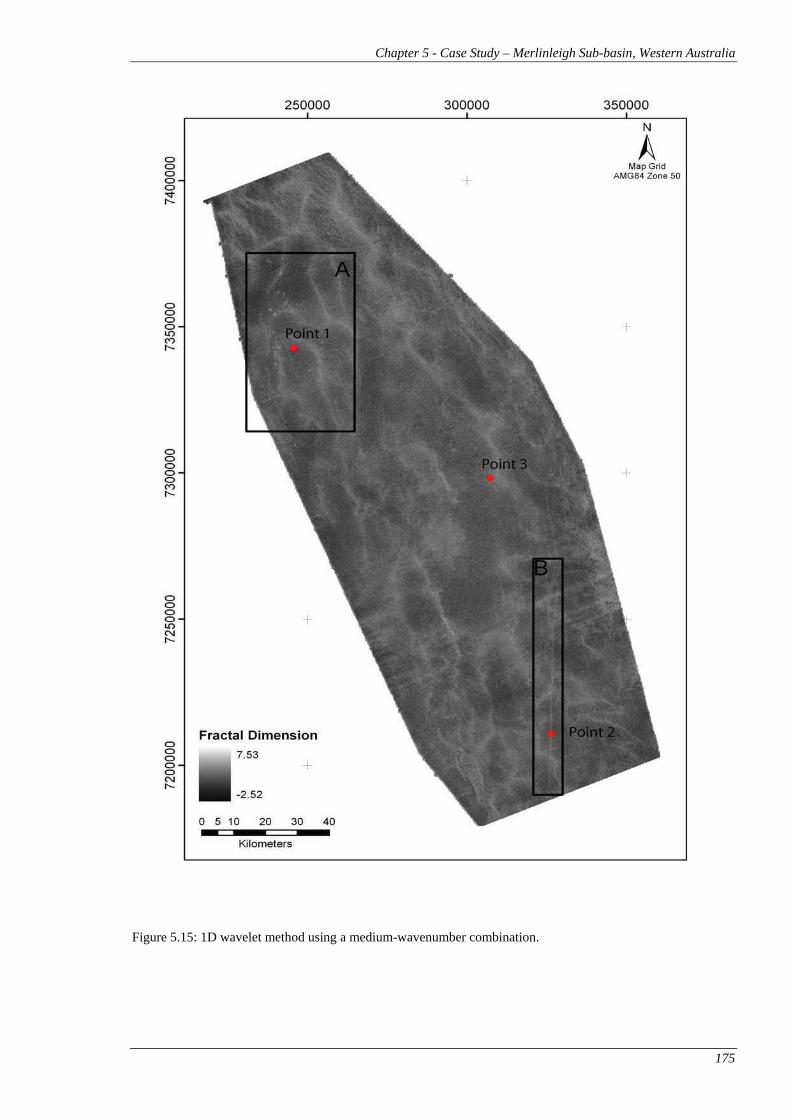
The 1D wavelet method was more effective than the 1D Gabor method at detecting features

such as the kimberlites and the Dampier-Pinjarra gas pipeline (labelled A and B respectively

in Figure 5.15). While these features are detectable in this image they are not as clearly

detectable as in any of the 2D fractal enhancements. The results are again dominated by

regions of ‘smeared’ high FD and flight line corrugations. Whilst this method performed

better than many of the other 1D fractal enhancements, it is worth noting that its range of FD

estimates is much broader than any of the other methods.


162

Figure 5.2: Colourdraped image of the RTP TMI with illumination from an azimuth of 315� and an inclination of 45�.


163

Figure 5.3: First vertical derivative of the RTP TMI.


164

Figure 5.4: Total horizontal derivative of the RTP TMI.


165

Figure 5.5: Analytic signal of the RTP TMI.


166

Figure 5.6: Image of the RTP TMI after applying automatic gain control with a window size of 7x7 points.


167

Figure 5.7: 2D variation method using a window size of 7x7 points.


168

Figure 5.8: 1D variation method using a window size of 31 points


169

Figure 5.9: 2D Hurst method using a window size of 9x9 points.


170

Figure 5.10: 2D semi-variogram method using a window size of 7x7 points.


171

Figure 5.11: 1D semi-variogram method using a window size of 31 points.


172

Figure 5.12: 2D Gabor method using a medium-wavenumber combination.


173

Figure 5.13: 2D wavelet method using a medium-wavenumber combination.


174

Figure 5.14: 1D Gabor method using a medium-wavenumber combination.


175

Figure 5.15: 1D wavelet method using a medium-wavenumber combination.


176

5.4 Discussion

The results presented in Section 5.3 demonstrate that the majority of the 2D FD estimation

methods effectively enhance high-wavenumber information in the Merlinleigh Sub-basin TMI

data. The methods are generally able to detect both the kimberlites in the north-west of the

image and the Dampier-Pinjarra gas pipeline in the south-east. Other high-wavenumber

features, such as the cross-cutting features in the outcrop to the east of the region, are also

enhanced. Moreover, all of these features are generally associated with large FD anomalies

and are consequently very easy to detect.

Some of the results for the FD methods presented above have estimates of FD that are outside

the theoretical range of one to two for 1D data and two to three for 2D data. Whilst magnetic

susceptibility may have a fractal distribution (Pilkington and Todoeschuck, 1993; Pilkington

and Todoeschuck, 1995), the associated magnetic field measured away from the source is

unlikely to be fractal due to the low-pass filtering effect associated with upward continuation.

This effect, combined with the use of localised rather than global estimates of FD, results in

estimates of FD outside of the appropriate theoretical ranges. However, as mentioned in

Chapter 1, the approach used within this thesis does not assume that airborne magnetic data

are truly fractal and consequently this issue does not influence the usefulness of FD as a

texture-based enhancement.

In order to better understand these FD results, examples of regression plots that have been

used to derive the FD estimates at Points 1, 2 and 3 on Figures 5.7 – 5.15 have been provided

(Figures 5.16 – 5.21). These points represent key features within the FD datasets, specifically

the kimberlites, the Dampier-Pinjarra pipeline and a region of generally low FD respectively.

The regression plots for the 1D methods come from the points on the original line data that

are closest to Points 1, 2 and 3.

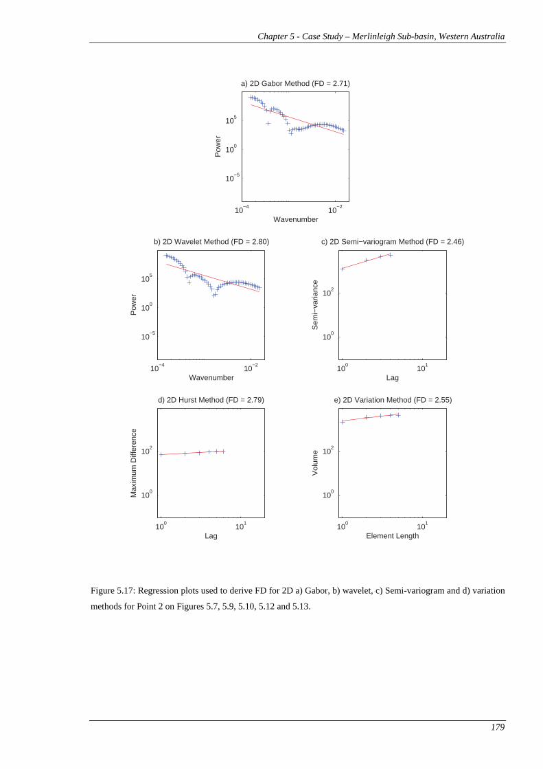
Figures 5.16 – 5.18 show the regression plots for the 2D methods and demonstrate that the

spectral methods (Figures 5.16a-b – 5.18a-b) generally have poorer quality regression fits

than the other 2D methods. However, there are many more points used in the estimation of

FD for the 2D spectral methods and this poorer quality of regression fit has not reduced their

effectiveness at enhancing the Merlinleigh data. Rather, the spectral methods sensitivity to a

broader bandwidth of features has allowed these methods to enhance additional features such

as the lineaments in the central region of the data (labelled C on Figures 5.12 – 5.13).


177

Figure 5.18 provides an example where most of the methods have estimates of FD outside of

the theoretical range of two to three. The exception here is the 2D variation method which

has an estimate of 2.21 (Figure 5.18e). These regression plots (Figure 5.18) are very similar

to those where the estimates of FD are within the correct theoretical range (Figures 5.16 –

5.18). Moreover, 2D spectral method regressions appear to be better fits than the regressions

for Points 1 and 2 even though their estimates of FD are less than two (Figure 5.18a-b).

Figures 5.19 – 5.21 show the regression plots for the 1D methods and demonstrate that the

spectral methods (Figures 5.19a-b – 5.21a-b) again generally have poorer quality regression

fits than the other 1D methods. Most of the examples provided here are within the allowable

theoretical range of FD for profiles, with the exception of the 1D variation method regressions

which are consistently less than 1 (Figures 5.19d – 5.21d).

Two-dimensional power spectra have been calculated in order to highlight and better explain

the differences between the various enhancements presented in Section 5.3 (Figures 5.22 –

5.24). These power spectra were calculated using the methodology described by Billings and

Richards (2001). Essentially, a thin-plate spline was used to fill in null values and a Kaiser-

Bessel window was then applied to eliminate spectral leakage1. All of the power spectra have

been normalised in order to allow for easy comparison.

Figure 5.22 presents the 2D power spectrum for each of the conventional enhancements

described in Section 5.3.1. The power spectrum for the RTP-TMI has a concentration of

energy around the centre of the power spectrum indicating a predominance of low-

wavenumber energy (Figure 5.22a). This supports the previous observation that the dataset is

relatively smooth and hence has little high-wavenumber energy. However, there is a distinct

band of power oriented in a top-right/bottom-left direction (Figure 5.22a) suggesting that the

data does contain some high-wavenumber features oriented perpendicular to this direction

(i.e. striking north-west/south-east). This is an intuitive result as the dominant strike of the

features in this region is north-west/south-east.

1 The code used for the calculation of 2D power spectra was provided by Dr Stephen Billings.


178

10−4 10−2

10−5

100

105

a) 2D Gabor Method (FD = 2.37)

Pow

er

Wavenumber

10−4 10−2

10−5

100

105

b) 2D Wavelet Method (FD = 2.67)

Pow

er

Wavenumber100 101

100

102S

emi−

varia

nce

Lag

c) 2D Semi−variogram Method (FD = 2.64)

100 101

100

102

Max

imum

Diff

eren

ce

Lag

d) 2D Hurst Method (FD = 2.69)

100 101

100

102

Vol

ume

Element Length

e) 2D Variation Method (FD = 2.52)

Figure 5.16: Regression plots used to derive FD for 2D a) Gabor, b) wavelet, c) Semi-variogram and d) variation

methods for Point 1 on Figures 5.7, 5.9, 5.10, 5.12 and 5.13.


179

10−4 10−2

10−5

100

105


Pow

erWavenumber

10−4 10−2

10−5

100

105


Pow

er

Wavenumber100 101

100

102

Sem

i−va

rianc

e

Lag


100 101

100

102

Max

imum

Diff

eren

ce

Lag


100 101

100

102

Vol

ume

Element Length





180

10−4 10−2

10−5

100

105


Pow

er

Wavenumber

10−4 10−2

10−5

100

105


Pow

er

Wavenumber100 101

100

102

Sem

i−va

rianc

e

Lag


100 101

100

102

Max

imum

Diff

eren

ce

Lag


100 101

100

102

Vol

ume

Element Length





181

10−4 10−2 100

100

105

Pow

er

Wavenumber


10−4 10−2 100

100

105

Pow

er

Wavenumber


100 101

10−2

100

102

Lag

Sem

i−va

rianc

e


100 101

100

101

102

Element LengthAr

ea

d) 1D Variation Method (FD = 0.84)


methods for Point 1 on Figures 5.8, 5.11, 5.14 and 5.15.

10−4 10−2 100

100

105

Pow

er

Wavenumber


10−4 10−2 100

100

105

Pow

er

Wavenumber


100 101

10−2

100

102

Lag

Sem

i−va

rianc

e


100 101

100

101

102

Element Length

Are

a





182

10−4 10−2 100

100

105P

ower

Wavenumber


10−4 10−2 100

100

105

Pow

er

Wavenumber


100 101

10−2

100

102

Lag

Sem

i−va

rianc

e


100 101

100

101

102

Element Length

Are

a


Figure 5.21: Regression plots used to derive FD for 1D a) Gabor, b) wavelet, c) semi-variogram and d) variation


The power spectra of the vertical and total horizontal derivatives and the analytic signal are all

similar to the RTP-TMI power spectrum (Figure 5.22a-d). All of these spectra have a

predominance of low-wavenumber energy although they have more high-wavenumber energy

than the RTP-TMI. All of these enhancements appear to have increased the previously

described high-wavenumber features, as demonstrated by the band of top-right trending high-

wavenumber energy being broader and stretching to higher wavenumbers (Figures 5.22b-d).

The AGC power spectrum has more high-wavenumber energy than any of the other

conventional enhancements (Figure 5.22e). This high-wavenumber energy is again contained

primarily within the top-right trending band of energy. However, in this case the power is

distributed to much higher wavenumbers than for any of the other conventional enhancements

(Figure 5.22e).


183

A comparison of the various 2D FD methods suggests that the geometric and stochastic

methods all provide relatively similar results across the dataset. There are some subtle

differences between these methods; however they broadly enhance the same features in the

Merlinleigh Sub-basin. This similarity is not surprising, as the methods all demonstrated

similar trends when applied to the synthetic datasets in Chapter 2 and 3.

The similarities between the 2D geometric and stochastic methods are also apparent in their

2D power spectra (Figure 5.23). All of these spectra are elongated towards the top-

right/bottom-left and they all have more energy to the top and bottom than any of the

conventional enhancements (Figure 5.23a-c). The principal difference between these spectra

is that the 2D semi-variogram spectrum tends to have more high-wavenumber energy than the

other two spectra. The semi-variogram method was applied using a smaller window size than

the 2D Hurst method, which would explain the increased high-wavenumber energy.

However, the 2D semi-variogram and variation methods were applied using the same window

size, hence any differences between these two spectra must be due to the fundamental

differences in their approach to estimating FD.

The 2D spectral methods (Figure 5.23d-e) are noticeably different to the 2D geometric and

stochastic methods (Figure 5.23a-c). The same general features are enhanced. However, the

2D spectral methods are better able to detect lineaments in the presence of extremely variable

data and have less regions of ‘smeared’ FD. The 2D spectral methods perform well in regions

of more variable data because of their ability to more precisely control the wavenumbers that

influence the FD estimation. The spectral methods use a series of estimates of the signal’s

power over a broad range of wavenumbers to calculate FD. This allows for far more

flexibility in ‘tuning’ the spectral methods to enhance specific features as opposed to the other

fractal-based methods that can only be controlled by the choice of window size.

The reduction in regions of ‘smeared’ FD is also seen in the spectral method’s power spectra

(Figure 5.16d). Whilst the 2D spectral methods have an increased amount of high-

wavenumber energy in the top-right/bottom-left direction, this band does not stretch to as far

as the other fractal-based enhancements.


184

Unlike the 2D FD methods, the 1D FD methods generally did not perform well on the

Merlinleigh Sub-basin data. The kimberlites and the Dampier-Pinjarra gas pipeline, which

were so clearly enhanced by most of the 2D methods, were barely detectable on any of the 1D

methods’ results. These results also tended to be dominated by smeared regions of high FD

that obscure most of the high-wavenumber features that were enhanced by the various 2D

methods.

As mentioned in Section 5.3, all of the 1D FD methods tended to enhance a series of flight-

line corrugations due to microlevelling problems with the Merlinleigh data. These features

are clearly seen in the associated power spectra as an increase in high-wavenumber energy

oriented from top-left to bottom-right (Figure 5.24). The only significant difference between

the 1D method’s power spectra is the reduced amount of high-wavenumber energy in the 1D

Gabor method (Figure 5.24 c). This lack of high-wavenumber energy is also evident in the

1D Gabor method results as the large regions of ‘smeared’ FD (Figure 5.14).

The 2D methods perform better than the 1D methods primarily because the 2D RTP-TMI

grids are smoother than the raw 1D data, due to the gridding process eliminating some of the

high-wavenumber content of the data. The removal of this high-wavenumber information

leads to datasets that are more suited to enhancement by fractal based techniques. This result

at first appears somewhat counterintuitive. The fractal based enhancements are all designed

to enhance high-wavenumber information, so why then does applying them to smoothed data

lead to better results? The answer is that the sensitivity of these methods makes them

susceptible to being overwhelmed by excessive amounts of high-wavenumber information.

Consequently, the methods work best when the data being examined are relatively smooth.

This result does not necessarily imply that there is no benefit in using the 1D methods. The

1D methods may well offer some advantages over the 2D methods in cases where the raw line

data are very smooth and the features of interest are of a very high-wavenumber. However, in

the case of the Merlinleigh Sub-basin dataset, the 2D methods clearly produced better results.


185

Figure 5.22: Two dimensional power spectra for the conventional enhancements described in Section 5.3.1. Specifically, power spectra are displayed for a) RTP-TMI, b) total horizontal derivative of the RTP-TMI, c) first vertical derivative of the RTP-TMI, d) analytic signal and e) AGC of the RTP-TMI.


186

Figure 5.23: Two dimensional power spectra for the 2D fractal enhancements described in Sections 5.3.2 - 5.3.4. Specifically, power spectra are displayed for the 2D a) variation, b) semi-variogram, c) Hurst, d) Gabor and e) wavelet methods.


187

Figure 5.24: Two dimensional power spectra for the 1D fractal enhancements described in Sections 5.3.2 - 5.3.4. Specifically, power spectra are displayed for the 1D a) variation, b) semi-variogram, c) Gabor and d) wavelet methods.

5.5 Conclusions

As mentioned in Section 5.1, the main aim of this chapter was to answer the following

questions:

1. Which of the FD estimation techniques effectively enhance the airborne magnetic data

from the Merlinleigh Sub-basin?

2. What are the key differences and similarities between the various FD estimation

techniques?

3. Are there significant differences between the results from the 1D and 2D methods of

estimating FD?


188

The answer to these questions are summarised below. Firstly, nearly all of the 2D FD

estimation techniques effectively enhanced the data from the Merlinleigh Sub-basin. The

methods all clearly enhance high-wavenumber information in the dataset, and when used in

conjunction with other enhancement techniques will provide valuable input into the

interpretation process. In contrast none of the 1D methods were particularly useful when

applied to this dataset and consequently they provide little information of benefit to the

interpretation process.

Secondly, the 2D geometric and stochastic methods produce similar results on this dataset.

There are subtle differences between the results of the various techniques, however there

appears to be only marginal benefit in producing all three enhancements (i.e. the variation,

semi-variogram and Hurst enhancements). The similarities between the two stochastic

methods are especially noticeable as the two techniques produce virtually identical results.

The key difference between these two methods was the choice of window size. The semi-

variogram method was applied with a slightly smaller window size than the Hurst method.

This suggests that the semi-variogram method may tend to be the better of the two methods as

the smaller window size allows high-wavenumber features to be better differentiated, and has

quicker processing times.

Thirdly, the results presented in this Chapter suggest that there is no significant advantage in

using 1D methods for this dataset. The creation of 2D grids involves smoothing which

removes some unwanted high-wavenumber noise. This in turn leads to smoother datasets that

are better suited to enhancement by fractal-based techniques. This result highlights another

key point regarding the use of fractal-based enhancements, which is that they appear to work

best on relatively smooth datasets. The problems that affected the 1D methods for this dataset

may well affect the 2D methods in regions where the airborne magnetic data are more

variable.

Documents

Chapter 5 Case Study – Merlinleigh Sub-basin, Western ... · a magnetic basement high (labelled B in Figure 5.2). Iasky et al. (1998) have also divided the magnetic basement into