Embed Size (px)
Citation preview

Aalborg University Institute of Energy Technology
Chapter 5 EMC and thermal analysis Abstract
This chapter deals mainly with problems related with the thermal analysis for the power
supply subsystem and for the whole satellite. A section about electromagnetic compatibility is also included. 5.1. Introduction ……....………………………………………………..………...……...….... Page 102 5.2. Thermal analysis ……………………………………………………………………….... Page 102 5.3. Methods of modeling …….…...………………………...……………………..…...……. Page 109 5.4. Thermal control ……………………...…………………………………………..……… Page 118 5.5. EMC considerations ………………………………………………………………...…… Page 120 5.6. Summary …………………………………………………………………..…………..… Page 123

EMC and thermal analysis
Page 102
5.1. Introduction
An important space in the present chapter is reserved for the thermal analysis. The
mechanisms of the heat transfer are presented, as well as some methods of thermal modeling and
control. It is important to have a control of the temperature inside the satellite, due to the hostile
environment in which the electronic components and other parts have to function. The analysis is
performed in several sections, starting with section 5.2.
Some basic knowledge about electromagnetic compatibility (EMC) is presented in section 5.5.
This part contains also some recommendations to follow in order to avoid electromagnetic
interferences and to minimize the parasitic emissions, due to digital circuits or power electronic
circuits.
5.2. Thermal analysis
One of the necessary parts of Cubesat’s design is the thermal analysis. It will provide us
operating temperatures an their distribution for all device inside satellite. For decision, which
temperature standard can be used for components it is necessary to know the maximum and the
minimum value of temperature. In virtue of this results the position of the all device must be also
optimized. Some methods for thermal control are also proposed. There are two main source of heat in
Cubesat, the Sun from outside and the electrical power from inside generated by all working
components
5.2.1. Conditions for Low Earth Orbit
In Chapter 2, section 2.4, the specifications for the Low Earth Orbit are described. As it has
been shown in section 2.3.1 (Table 2.1), the heat in space comes from three main sources:
The Sun – energy 1358±5 [W/m2]
Albedo – energy 406 [W/m2]
Infrared – energy 237 [W/m2]
The temperature surrounding the satellite in space is 2.7K and the pressure surrounding is very close
to vacuum. In figure 5.1, are illustrated the sources of heat in space [Sellers, p.67, 1994].

Thermal analysis
Page 103
Figure 5. 1 Sources of radiation in space
5.2.2. Heat transfer
There are three mechanisms by which thermal energy is transported:
1. Convection
2. Conduction
3. Radiation
In space convection can be neglected. As said before, the surrounding temperature in space is 2.7˚K,
very close to absolute zero. Then there is no transfer between hot and cold air as on the Earth. The
vacuum is also cause for this problem, because there is no difference in density of gasses.
Conduction
In definition of heat transferred through conduction, the following formula is used:
LTAPcond
∆⋅⋅λ= (5.1)
where λ is thermal conductivity [J/s⋅m⋅K]
A is a cross section area [m2]
L represents the length of the conduction path [m]
∆Τ is difference temperatures between the two bodies, T1 and T2
In figure 5.2 is shown an illustration of the heat conduction mechanism.
Thermal resistance is defined by formula:
[ ]K/W_cond
condth PTR ∆= (5.2)

EMC and thermal analysis
Page 104
Figure 5.2 Illustration of heat conduction mechanism
[http://sol.sci.uop.edu/~jfalward/heattransfer/heattransfer.html] Replacing the expression of Pcond from equation (5.1), it yields:
[ ]K/W_ ALR condth ⋅λ
= (5.3)
Conduction will apply only for components on the same board and Rjc (thermal resistance
junction case) can be assumed as a thermal resistance for this transfer.
Radiation
All matter and space contains electromagnetic radiation. A particle of electromagnetic energy
is a photon, and heat transfer by radiation can be viewed either in terms of electromagnetic waves or
in terms of photons.
For calculation of the amount of heat transferred through radiation is valid Stefan-Boltzmann
law:
4 TAPrad ⋅⋅σ⋅ε= (5.4)
where, ε = emissivity (value between 0÷1)
σ = Stefan-Boltzmann constant equal with 5.67⋅10-8 [W/m2K4]
A = surface area of object [m2]
T = temperature [K]
From this equation may be observed that for modifying the radiated power for an object, the only
parameter which can be changed is the emissivity of radiating object, supposing that the object
maintains its physical dimensions. This can be realized by modifying the color and surface of
component. Figure 5.3 shows the difference between the absorbtion and emission of radiation.
[http://sol.sci.uop.edu/~jfalward/heattransfer/heattransfer.html]
For a dark-color material, the absorbtion of a radiated amount of heat is higher than for a light-color
material, supposing the same geometric dimensions for the two bodies.

Thermal analysis
Page 105
Figure 5.3 Absorption and emission of radiation
The thermal resistance for radiation can be defined as:
[ ]K/W_rad
radth PTR ∆= (5.5)
Combining equations (5.4) and (5.5), the thermal resistance may be written in the following form:
[ ]K/W1_ Ah
Rr
radth ⋅= (5.6)
where, 34 mr Th ⋅σ⋅ε⋅= is called the radiation heat transfer coefficient [W/m2K].
For normal room temperature, 25°C (= 298K), hr is about six times the surface emmitance. This can
be easily proved, replacing in the definition relation the corresponding numbers [Mills, p.16, 1995]:
K][W/m 6]K[)298(]KW/m[1067.54 23428 ε⋅≅⋅⋅⋅ε⋅= −rh (5.7)
5.2.3. Temperature equilibrium
A temperature equilibrium will be always reached after the solar irradiation has begun. It is
helpful to know this temperature for the first idea about thermal conditions in the Cubesat. There is
presented only instance without internal heat sources. The temperature equilibrium is obtained when
the absorbed power QA is equal to emitted power by radiation QE. These values are given by the
following equations:
inA ASQ ⋅α⋅= 0 (5.8a)

EMC and thermal analysis
Page 106
4eoutE TAQ ⋅⋅σ⋅ε= (5.8b)
where the symbols in the equations have the following significances:
S0 is solar irradiation (1353 [W/m2], in case of sunlight, 237 [W/m2], in case of eclipse),
α represents the absorbitivity of the material,
Ain is area illuminated by solar irradiation [m2],
ε is the emissivity of the material,
σ is Stephan-Boltzmann constant, equal with 5.67 x 10⁻⁸ [W/m2K4],
Aout is the radiating area [m2], and
Te represents the equilibrium temperature [K].
The equilibrium temperature is obtained from condition QA = QE. Replacing the expressions for the
two amounts of heat, from equations (5.8a, b), it yields:
40
σ⋅
εα⋅=
SAA
Tout
ine (5.9)
In the satellite are used these materials with their constants as is shown in table follows.
Solar cells (InGaP,GaAs,Ge)
Material of sides (Carbon)
Material on side with camera (Aluminum)
α 0.75 0.96 0.55 ε 0.83 0.9 0.3
Coverage of one side (%) 57 43 100
Table 5.1 Absorbitivity and emissivity for materials used in the satellite Case of sunlight
Solar irradiation is taken into account without respect of Albedo and infrared heat from the
Earth. The illuminated sides are only the sides with solar cells (side with camera is still pointed to the
Earth). For material constants can be put only values with respect of coverage of sides. It can be
calculated as below:
8403.043.096.057.075.043.057.0 =⋅+⋅=⋅α+⋅α=α matcell (5.10a)
8601.043.09.057.083.043.057.0 =⋅+⋅=⋅ε+⋅ε=ε matcell (5.10b)
Due to assumption, that the satellite will stay in position with camera side pointed to the Earth, there
are these boundary conditions:
• One side illuminated
• Three sides illuminated

Thermal analysis
Page 107
From equations (5.10a, b) the equilibrium temperature can be calculated as follows:
( )4 04 0
1
1
1515 σ⋅ε⋅+ε⋅⋅α⋅
=σ
⋅ε⋅+ε⋅
α⋅⋅=camcam
eSNS
AANT (5.11)
where A1 is the area of one side [m2],
N is number of illuminated sides, and
εcam represents the emissivity of material on side with camera.
The illuminated area is dependent on the angle of sunlight and its maximum is respected by N
(section 3.3.1). That is why this value is placed in numerator.
In radiation must be taken in account that all of sides are radiating. But not all of them are the
same. One side (with camera) has different conditions. This is a reason for writing such a shape of
denominator as in equation (5.11).
Then by inserting these values into the equation (5.11) is obtained:
One side illuminated:
( ) C][19.18K][94.256]K[W/m1067.53.018601.05
][W/m13538403.0 o4428
2
−==⋅⋅⋅+⋅
⋅= −eT (5.12)
Three sides illuminated:
( ) C][62.21K][77.294]K[W/m 1067.53.018601.05
][W/m13538403.03 o4428
2
==⋅⋅⋅+⋅
⋅⋅= −eT (5.13)
Three sides illuminated simultaneously by direct solar irradiation, Albedo, infrared heat of
the Earth:
( )( ) C][84.54K][99.327
]K[W/m 1067.53.018601.05][W/m 23740613538403.03 o4428
2
==⋅⋅⋅+⋅++⋅⋅= −eT (5.14)
Case of eclipse
The source of power for this case is only infrared heat produced by the Earth by itself. In this
case are counted all possible boundary conditions that can appear:
• One side pointed to the Earth
o Side with camera (case 1)
o Side without camera (case 2)
• Three sides pointed to the Earth
o Including side with camera (case 3)

EMC and thermal analysis
Page 108
o Without side with camera (case 4)
In all of these cases is the denominator still the same due to radiation of all sides. Then the general
equation can be written as follows:
( )
( )4
0´
15 σ⋅ε⋅+ε⋅
⋅α⋅+α⋅⋅++
=cam
camcamcellscellscam
cellscam
e
SNNNNNN
T (5.15)
where Ncam = 1 if the side with camera is illuminated,
0 if the side with camera is not illuminated,
Ncells is the number of sides with cells illuminated,
α is the absorbtivity with respect of coverage,
ε represents the emissivity with respect of coverage,
αcam is the absorbtivity of side with camera,
εcam is the emissivity of side with camera,
S0 = 237 [W/m2] represents the irradiation due to infrared heat from the Earth, and
σ is Stephan-Boltzmann constant (5.67 x 10⁻⁸ [W/m2K4]).
Then by inserting these values into the equation (5.15) the following results are obtained:
case 1: ( )
( ) ]C[ 64.123[K] 51.149]KW/m[1067.53.018601.05
]W/m[23755.018403.000101
o4428
2
−==⋅⋅⋅+⋅
⋅⋅+⋅⋅++
= −eT (5.16)
case 2: ( )
( ) ]C[92.106K][23.166]KW/m[1067.53.018601.05
]W/m[23755.008403.011010
o4428
2
−==⋅⋅⋅+⋅
⋅⋅+⋅⋅++
= −eT (5.17)
Case 3: ( )
( ) ]C[2.88]K[95.184]KW/m[1067.53.018601.05
]W/m[23755.018403.022121
o4428
2
−==⋅⋅⋅+⋅
⋅⋅+⋅⋅++
= −eT (5.18)
Case 4: ( )
( ) ]C[46.82]K[69.190]KW/m[1067.53.018601.05
]W/m[23755.008403.033030
o4428
2
−==⋅⋅⋅+⋅
⋅⋅+⋅⋅++
= −eT (5.19)
Conclusion
The goal was to compute the equilibrium temperature for the satellite, considering no internal
heat sources. If all equilibrium temperatures are compared than can be seen that the worst case for the
satellite is in eclipse when only side with camera is pointed to the Earth.

Methods of modeling
Page 109
Then, it is accepted the smallest amount of energy in comparison with other cases. In addition,
in all cases are radiating all sides. But must be mentioned, that no internal heat made by equipments is
taken into account. So temperature range according to the temperature equilibrium is:
Tmax = 55 [˚C]
Tmin = -124 [˚C]
From this numbers can be derived that satellite has a trend to keep lower temperature than higher one.
This is advantage for us, because no internal sources of heat are included. Internal heat sources will
raise temperature inside.
5.3. Methods of modeling 5.3.1. Two-dimensional model of board
In this part of analysis the method of modeling for the electrical board is suggested. Whole
Cubesat will be divided into separate layers, corresponding to the number of boards and each layer
will be meshed, as shown in figure 5.4.
Figure 5.4 Meshed layer of the satellite
Then the components from the board will be projected into the mesh such a way, that thermal source
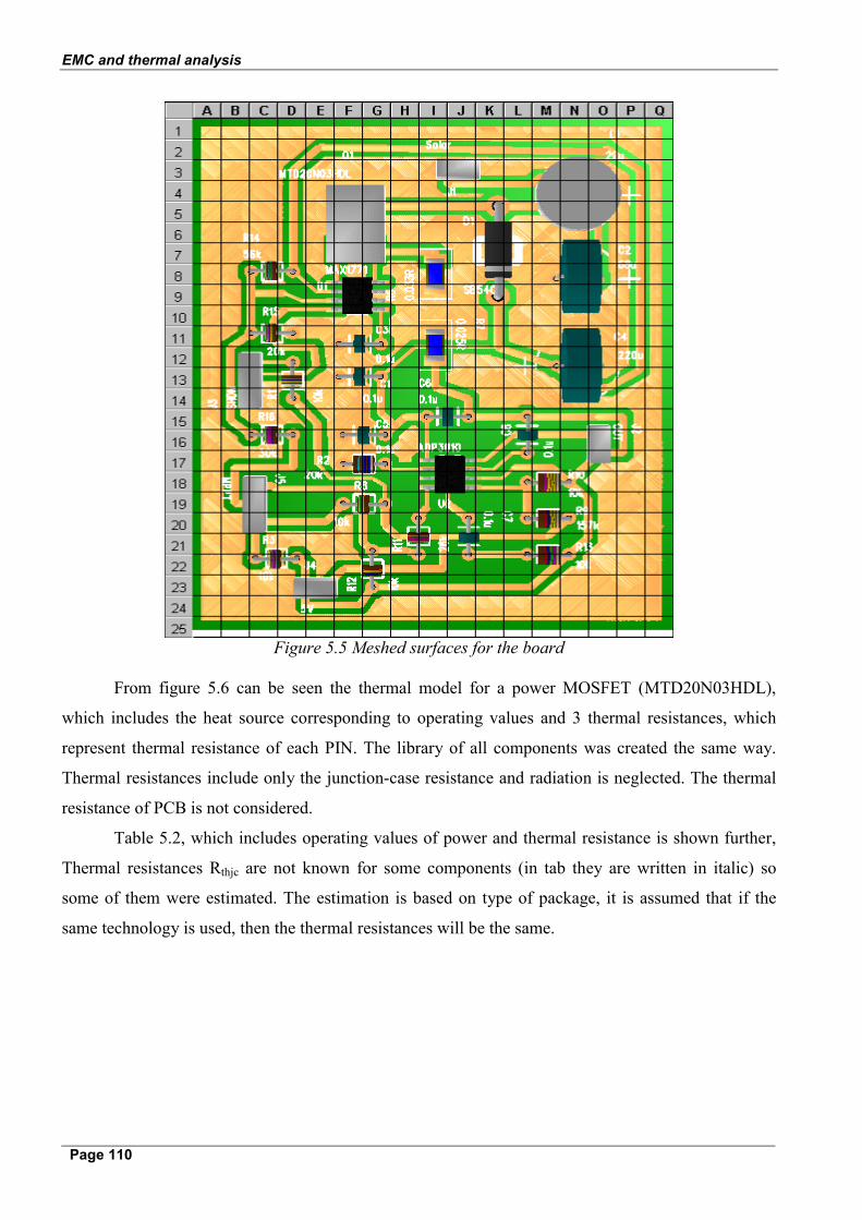
and thermal resistances will represent each component. An example is depicted in figure 5.5. The
thermal models for the components are implemented by use of Saber software. On the attached CD-
ROM can be found all files concerning this simulation.
EMC and thermal analysis
Page 110
Figure 5.5 Meshed surfaces for the board
From figure 5.6 can be seen the thermal model for a power MOSFET (MTD20N03HDL),
which includes the heat source corresponding to operating values and 3 thermal resistances, which
represent thermal resistance of each PIN. The library of all components was created the same way.
Thermal resistances include only the junction-case resistance and radiation is neglected. The thermal
resistance of PCB is not considered.
Table 5.2, which includes operating values of power and thermal resistance is shown further,
Thermal resistances Rthjc are not known for some components (in tab they are written in italic) so
some of them were estimated. The estimation is based on type of package, it is assumed that if the
same technology is used, then the thermal resistances will be the same.

Methods of modeling
Page 111
Figure 5.6 Thermal model for a power transistor
Working conditions Component
name Function
Number of
pieces
Number of
legs
Rth j-c (K/W) Current
(A) Voltage
(V) Power
(W)
Included in
model?
MTD20N03HDL switch for
step-up convertor
1 3 1.67 0.58 5.23 3 yes
NDT 456P switch for step-down convertor
1 3 12 2 3.4 6.8 yes
TPS2034 protection
for transmitter
1 8 10 1.8 5 9 yes
TPS2030
protection for
ACS,CAM, MCU, OBC
4 8 10 0.05; 0.06;
0.003; 0.092
5 0.25; 0.3;
0.015; 0.46
yes
MAX1771 step-up convertor 1 8 10 110µ 5 0.55m yes
MAX1744 step-down convertor 1 8 10 221µ 8.4 1.86m yes

EMC and thermal analysis
Page 112
UCC3911
protection for 2
batteries in series
2 16 12 0.92 8.4 7.728 yes
SB540 diodes for convertors 2 2 2 0.5 0.43 0.215 yes
PRLL5817 string diodes for solarcells 5 2 5 0.5 0.35 0.175 yes
MAX4372 current-sence amplifier 10 5 7 30µ 5 0.15m no
LM78L05 terminal positive regulator
1 8 7 0.1 5 0.5 yes
MAX835 latching voltage monitor
4 5 7 15µ 5 0.075m no
Table 5.2 Operating values of components
From these components MAX4372 and MAX835 were neglected.
The restrictions of 2D model are stated as follows:
• The thermal resistance of PCB is not considered.
• Number of nodes is directly connected to the accuracy of the model. The more nodes we
have the higher accurate model we obtain.
• In our case only main sources of heat will be taken in account.
• Radiation is not included in this model; it is supposed that the conduction through the
copper is main way for heat transfer.
• Distances between components are not included.
• The model is only two-dimensional and it is a problem to transfer into 3D.
• The thermal resistances for radiation (Rthca case-ambient) are not included in datasheets
and must be computed for each component.
• Saber software is not optimal for this type of analysis.
• Creating of the model is elaborate and requires a large amount of work.
• Thermal resistances Rthjc are not known for all device.

Methods of modeling
Page 113
5.3.2 Implementation of the model and results
The whole thermal model of the PSU board is depicted in figure 5.7. In model there are
included only main sources of heat. Position of components is respecting the electrical layout, because
final board wasn’t at disposal. It is assumed that the copper on a board is conducting the most of the
heat, because its thermal conductivity is thousand times higher then for the board. Pins, which are not
connected to other components and have no function have zero value. If it is not like this, the Saber
software will assume them as a nonfinite value and it will alter the results.
Figure 5.7 Final layout for thermal model
The results are presented in table 5.3 and in figure 5.8.
All temperatures are acceptable and are following the industrial standard. The highest temperature is
on the switch of step-down converter (40.9˚C). It is exactly according to the expectances, because of
the highest power. Also protections for batteries and for communication module will have
temperatures near to 20˚C.

EMC and thermal analysis
Page 114
Device Temperature (oC)
Step-up 13.3 Convertors Step-down 5.3 ACS 3.1
Batteries 16.6 CAM 3.2 MCU 2.8 OBC 3.4
Protections
Transmitter 15.6 String 4.9
SB540 for step-up 11.3 Diodes SB540 for step-down 3.4
For step-up 13.6 Switches For step-down 40.9 Terminal positive regulator 5.0
Table 5.3 temperatures of main components
0.05.0
10.015.020.025.030.035.040.045.0
Step
-up
Step
-dow
nAC
SBa
tterie
sC
AMM
CU
OBC
Tran
smitt
erSt
ring
SB54
0 fo
rSB
540
for
For s
tep-
For s
tep-
Term
inal
Device
Temperature (oC)
Figure 5.8 Temperatures of main components
Conclusion
Sequent model is not the final one, because it does not consider the geometrical distribution of
components. For successful completion of it, the final board is necessary. The method for it, is shown
in figure 5.5. The model has many restrictions and imperfections. The main problem is that the
material properties of the board are not included and if two components are very close and their
electrical connection is far distant then the conduction by board can apply more than by copper.

Methods of modeling
Page 115
Anyway, this model gives the basic idea about thermal conditions on a PSU board. The main
sources of heat and the temperature amount are known. The problem is with verifying values of
resulting temperatures in our laboratory. For this it is necessary to eliminate convection so vacuum
chamber is needed. It is also clear that the temperatures are strongly dependent on thermal resistances,
which were just estimated. 5.3.4. Three-dimensional model of satellite
In reference to mentioned restrictions of previous model, another solution for 3D model
needed to be found. In this case, a software using method of finite elements have to be used. ANSYS
software has been chosen as a most suitable for our application. Its biggest advantage is that it
consider the material properties and it works in three dimensions. On the other hand it is very
sophisticated tool and it requires a lot of time to learn it.
To simplify the realization of model it will include only main parts of the satellite:
• Side walls
• Solar cells
• It is assumed steady state for all the computations
For proper function of this software, it is necessary to choose a proper element. As was
mentioned before, between heat conduction mechanisms, only radiation and conduction are applicable
in a space application. For a 3D analysis only LINK31, SHELL57 and SURF152 elements can work
in ANSYS software with respect to radiation.
LINK31 element can be used only for calculating the heat flow between two nodes. It only has
these two nodes and cannot be meshed. SHELL57 has four nodes and capability to define in each
node different thickness. There is not problem with meshing of this element.
SURF152 (also called superelement) may be used for various load and surface effect
applications.
If a radiation simulation between some surfaces and surroundings has to be performed, then
the SHELL57 element must be chosen. After setting the thickness, the geometry of the satellite can be
done by creating key points, from them lines and finally from lines can be constructed areas of each
hand side. Figure 5.9 shows an example of a meshed surfaces for the satellite.

EMC and thermal analysis
Page 116
Figure 5.9 Example of meshed structure for the satellite
Following, there are two methods of doing simulation with reference to radiation problem:
• AUX12 Radiation Matrix Method
• Radiosity Solver Method.
For the AUX12 method must be SHELL57 superimposed by superelement on which must be defined
conditions for radiation.
Assigning edge conditions for the model
Because there was not possible to establish temperature distribution only from heat flux and
material properties, boundary conditions had to be calculated.
For calculation the edge temperature on the sun side (T1), can be used Stefan-Boltzmann law:
εσ ⋅⋅= 4TSrad (5.20)
From this, the expression of temperature resides:
4
εσ ⋅= radS
T (5.21)
where the symbols in the equations have the following significances:
Srad is the solar heat flux, equal with 1353 [W/m2]
ε is the emissivity of the material, and
σ is Stephan-Boltzmann constant, equal with 5.67 x 10⁻⁸ [W/m2K4].

Methods of modeling
Page 117
Assuming the emissivity ε equal with 1, and replacing the numbers in equation (5.21), it yields:
]C[120]K[393]KW/m[1067.51
]W/m[13534
428
2
1 ==⋅⋅
= −T (5.22)
A similar value can be obtained also by computing thermal equilibrium for solar cells. The same
equation can be used for infra radiation from the side of the Earth, only now the heat flux for infrared
is 237 [W/m2].
]C[19]K[254]KW/m[1067.51
]W/m[2374
428
2
2 −==⋅⋅
= −T (5.23)
By using these edge conditions it has been obtained the picture shown in figure 5.10 (using SHELL57
element), which shows temperature distribution in Cubesat, but this model is including only
conduction. It is necessary to build similar model for radiation, but this was not possible at the time of
doing the analysis.
Figure 5.10 Distribution of temperature on the satellite surface
Conclusion
The built model is very simple and couldn’t satisfy our recommendations. It is necessary to
find a solution for radiation element. And connect both models together.

EMC and thermal analysis
Page 118
5.4. Thermal control
It is necessary to keep the temperature in Cubesat during the mission in the industrial standard,
because all electronic devices are designed to operate in this temperature range. The methods of
realizing this goal are described in the following.
The methods of thermal control can be split into two categories, passive methods and active
methods. In respect to the size of the satellite, passive methods will be preferred.
Heat insulation is needed to keep an instrument sufficiently warm or to prevent heat from
body-mounted solar panels from propagating into the spacecraft or for separation the heat-sensitive
parts. Used material is MLI (multilayer insulation), with a structure like the one depicted in figure
5.11 [Hansen, 2001].
Figure 5.11 Thermal insulating material
This material is very light and thin and can be simple used for a small satellite. This material will be
probably used as a thermal shielding for our batteries. This can help us to avoid fast temperature
changes.
Another passive form is changing value of α/ε factor. This can be realized by changing the
color or surface materials. This method is very easy to implement and is also reliable. Temperature
equilibriums for different values of α/ε factor can be seen in a table 5.4 [Hansen, 2001].
No. Material Measure-
ment temp.(K)
Surface condition
Solar absorbitivity
α
Infrared emissivity
ε
α/ε ratio
Equili-brium
temp.(oC)
1 Aluminum (6061-T6) 294 As received 0.379 0.0346 10.95 450
2 Aluminum (6061-T6) 422 As received 0.379 0.0393 9.64 428
3 Aluminum (6061-T6) 294 Polished 0.2 0.031 6.45 361
4 Aluminum (6061-T6) 422 Polished 0.2 0.034 5.88 346
5 Gold 294 As rolled 0.299 0.023 13.00 482

Thermal control
Page 119
6 Titanium (6AL-4V) 294 As received 0.766 0.472 1.62 176
7 Titanium (6AL-4V) 422 As received 0.766 0.513 1.49 166
8 Titanium (6AL-4V) 294 Polished 0.448 0.129 3.47 270
9 Titanium (6AL-4V) 422 Polished 0.488 0.148 3.30 251
10 White enamel 294 Al. substrate 0.252 0.853 0.30 20
11 White epoxy 294 Al. substrate 0.248 0.924 0.27 13
12 White epoxy 422 Al. substrate 0.248 0.888 0.28 16
13 Black paint 294 Al. substrate 0.975 0.874 1.12 136
14 Silvered Teflon 295 0.08 0.66 0.12 -39
15 Aluminized Teflon 295 0.163 0.8 0.20 -6
16 Quartz Over Silver 295 0.077 0.79 0.10 -51
17 Sol.Cell-Fused Silica Cover 0.805 0.825 0.98 122
18 Crushed Carbon Graphit 0.88 0.96 0.92
Table 5.4 Temperature equilibrium for different materials
From the active methods of thermal control, the rotating method can be mentioned. If large
amounts of heat are located on a board the satellite, this can start slowly to rotate. There exists a
critical value of temperature, which can be measured by temperature sensors and this signal can be
used as a control signal for the attitude control system to rotate the satellite. This method is dependent
on speed of rotation, which is connected to the induced current into the magnetotorquers. We cannot
rotate very fast or very slow, the speed of rotation must be optimized in transient thermal analysis.
And it is a task for thermal stabilization.
Also heaters are used to avoid low temperatures. They can be realized as electrical blankets or
as small resistances. For our application they seem to be so inefficient, because of power problems.
Only one possible application can be realized for heating batteries. The necessary amount of the heat
has to be computed.
Heat pipes are the last active method. Heat pipes can transfer much higher powers for a given
temperature gradient than even the best metallic conductors. They are hollow tubes closed on both
ends filled with some fluid like ammonia, as shown in figure 5.12. As one end of the pipe is exposed
to a heat source, the ammonia absorbs this heat and vaporizes. The ammonia vapor then flows through

EMC and thermal analysis
Page 120
the pipe and carries the heat away to the cold end. There the ammonia losses its heat and recondenses
as a liquid. It then flows back to the other end. This is a form of convection in which the work is being
done not by gravity but by the wicking effect. This system can be effective for higher temperatures,
depends on boiling point of inner fluid. (But in case of our system the problem is to avoid low
temperatures during the eclipse). Its light weight (generally less than 40 grams), small, compact
profile, and its passive operation, allow it to meet the demanding requirements of mini satellites. Their
application needs deeper analysis. They can be used for transporting heat from hot (illuminated) sides
to cold one.
Figure 5.12 Heat pipes – principle of operation
[http://www.electronics-cooling.com/Resources/EC_Articles/SEP96/sep96_02.htm] 5.5. EMC considerations Power supply must also fulfill requirements for EMC. It means that the level of the electromagnetic
noise of our device should be below admissible value for other parts of Cubesat. And on the other
hand our device must be resistant enough against foreign sources of noise
[http://www.its.bldrdoc.gov/fs-1037/dir-013/_1932.htm].

EMC considerations
Page 121
Definitions
Electromagnetic compatibility (EMC):
1. Electromagnetic compatibility is the condition, which prevails when equipment is
performing its individually designed function in a common electromagnetic environment without
causing or suffering unacceptable degradation due to unintentional electromagnetic interference to or
from other equipment in the same environment.
2. The ability of systems, equipment, and devices that utilize the electromagnetic spectrum to
operate in their intended operational environments without suffering unacceptable degradation or
causing unintentional degradation because of electromagnetic radiation or response. It involves the
application of sound electromagnetic spectrum management; system, equipment, and device design
configuration that ensures interference-free operation; and clear concepts and doctrines that maximize
operational effectiveness.
Electromagnetic environment (EME):
1. For a telecommunications system, the spatial distribution of electromagnetic fields
surrounding a given site. The electromagnetic environment may be expressed in terms of the spatial
and temporal distribution of electric field strength [V/m], irradiance [W/m2], or energy density [J/m3].
2. The resulting product of the power and time distribution, in various frequency ranges, of
the radiated or conducted electromagnetic emission levels that may be encountered by a military
force, system, or platform when performing its assigned mission in its intended operational
environment. It is the sum of electromagnetic interference; electromagnetic pulse; hazards of
electromagnetic radiation to personnel, ordnance, and volatile materials; and natural phenomena
effects of lightning.
Electromagnetic interference (EMI):
1. Any electromagnetic disturbance that interrupts, obstructs, or otherwise degrades or limits
the effective performance of electronics/electrical equipment. It can be induced intentionally, as in
some forms of electronic warfare, or unintentionally, as a result of spurious emissions and responses,
intermodulation products
2. An engineering term used to designate interference in a piece of electronic equipment
caused by another piece of electronic or other equipment. EMI sometimes refers to interference
caused by nuclear explosion [JP 1-02].
Level of noise
• High frequencies >1MHz
• Low frequencies our case <1MHz
EMC and thermal analysis
Page 122
Digital circuits as a noise sources
Digital circuits generate mainly narrow-band noise, that means energy is concentrated on single
frequency. The biggest emission is normally between 50 and 500 MHz depends on clock frequency.
The highest energy appears normally as a harmonic of clock frequency. Our microcontroller works on
1MHz. There is also direct emission from the PCB, which works as a magnetic loop antenna. The
emission level depends on the current in the loop. From this is obvious that the board must be as small
as possible. It is also important to use a PCB with ground plan (gridded ground system).
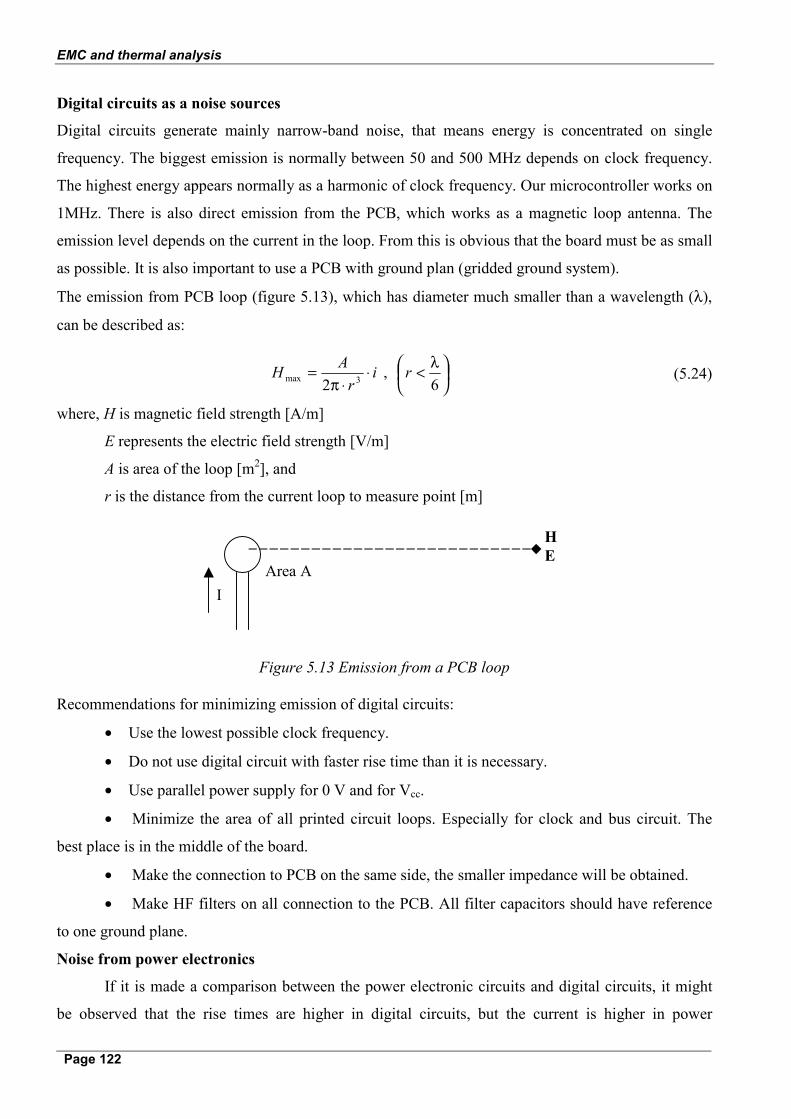
The emission from PCB loop (figure 5.13), which has diameter much smaller than a wavelength (λ),
can be described as:
ir
AH ⋅⋅π
= 3max 2 ,
λ<
6r (5.24)
where, H is magnetic field strength [A/m]
E represents the electric field strength [V/m]
A is area of the loop [m2], and
r is the distance from the current loop to measure point [m]
Area A I
H E
Figure 5.13 Emission from a PCB loop
Recommendations for minimizing emission of digital circuits:
• Use the lowest possible clock frequency.
• Do not use digital circuit with faster rise time than it is necessary.
• Use parallel power supply for 0 V and for Vcc.
• Minimize the area of all printed circuit loops. Especially for clock and bus circuit. The
best place is in the middle of the board.
• Make the connection to PCB on the same side, the smaller impedance will be obtained.
• Make HF filters on all connection to the PCB. All filter capacitors should have reference
to one ground plane.
Noise from power electronics
If it is made a comparison between the power electronic circuits and digital circuits, it might
be observed that the rise times are higher in digital circuits, but the current is higher in power

Summary
Page 123
electronics. This can lead to emission of high levels of noise and electromagnetic interferences, if
proper methods to avoid this are not considered.
Recommendations to prevent noise: • Loops in circuit as short as possible: long loops works by certain frequencies as magnetic
loop antenna.
• Shielding: It reduces or absorbs the coupling between noise source and the victim. The
cause of this effect is, that the conductive shield hit by electromagnetic field will induce current in the
plate, which transform the field energy into the heat.
The damping ability of a shield depends on:
• The frequency of the field
• The field impedance
• The shield material
• The dimensions and the placing of the shield
Absorption loss in shield are given by the following formula:
tfA rr ⋅σ⋅µ⋅= 131 (5.25)
where, f represents the frequency of electromagnetic signal [Hz]
μr is the relative permeability of shield material
σr is the material relative conductivity in relation to copper, and
t represents the shield thickness.
Reflection loss are given as:
[ ]dB 1log10168
⋅
µσ
+=f
Rr
r (5.26)
where, f is the frequency of the perturbing signal [Hz],
σr is the material relative conductivity in relation to copper, and
μr represents the relative permeability of shield material
5.6. Summary
The goal of thermal analysis developed in this chapter, is to have basic idea about temperature
distribution in Cubesat and suggest some methods for thermal control. For this different approaches
were used. First of all was computed the temperature equilibrium for the satellite, considering no
EMC and thermal analysis
Page 124
internal heat sources. If all equilibrium temperatures are compared than can be seen that the worst
case for Cubesat is in eclipse when only side with camera is pointed to the Earth. So temperature
range according to the temperature equilibrium is:
Tmax = 55 [˚C]
Tmin = -124 [˚C]
From this numbers can be derived that satellite has a trend to keep lower temperature than higher one.
This is advantage for us, because no internal sources of heat are included and they will raise
temperature inside.
Second part was model of the board in Saber , which gives us basic idea about temperatures on
a board. Highest obtained temperature for switch of step-down converter is 40.9˚C, which is far away
from maximum for industrial standard. Of course, this temperatures will add up with the temperatures
of surroundings and they are not final.
Next most problematic part was model of whole Cubesat in ANSYS: The built model is very
simple and couldn’t satisfy our recommendations. It is necessary to find a solution for radiation
element. And connect both models together.
From thermal control shielding for batteries is suggested (as the most temperature sensitive
part of power subsystem). MLI can be easily used for this. Also heat pipes seem to be relevant for the
current application.
Some basic considerations about electromagnetic compatibility problems are presented in
section 5.5. Potential sources of noise are analyzed and a comparison between them is made.
Measurement of noise for final board on spectrum analyzer will be done.


![[EMC 311] Chapter 2 Getting Around Linux on Raspberry Pi](https://img.pdfslide.net/doc/110x75/577cd81d1a28ab9e78a070b2/emc-311-chapter-2-getting-around-linux-on-raspberry-pi.jpg)