Embed Size (px)
Citation preview
Chapter 5
Graphing and Optimization
Section 4
Curve Sketching Techniques

2
Objectives for Section 5.4 Curve Sketching Techniques
■ The student will modify his/her graphing strategy by including information about asymptotes.
■ The student will be able to solve problems involving modeling average cost.

3
Modifying the Graphing Strategy
When we summarized the graphing strategy in a previous section, we omitted one very important topic: asymptotes. Since investigating asymptotes always involves limits, we can now use L’Hôpital’s rule as a tool for finding asymptotes for many different types of functions. The final version of the graphing strategy is as follows on the next slide.
4Barnett/Ziegler/Byleen Business Calculus 12e
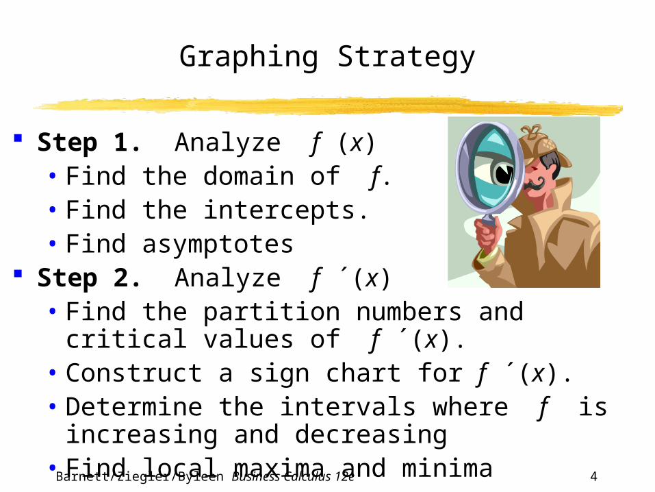
Graphing Strategy
Step 1. Analyze f (x)• Find the domain of f.• Find the intercepts.• Find asymptotes
Step 2. Analyze f ´(x)• Find the partition numbers and critical values of f ´(x).• Construct a sign chart for f ´(x).• Determine the intervals where f is increasing and
decreasing• Find local maxima and minima
5
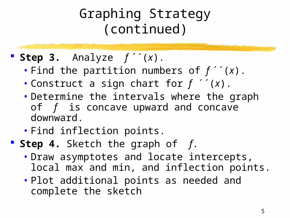
Graphing Strategy(continued)
Step 3. Analyze f ´´(x).• Find the partition numbers of f ´´(x).• Construct a sign chart for f ´´(x).• Determine the intervals where the graph of f is
concave upward and concave downward.• Find inflection points.
Step 4. Sketch the graph of f.• Draw asymptotes and locate intercepts, local max
and min, and inflection points.• Plot additional points as needed and complete the
sketch
6
Example
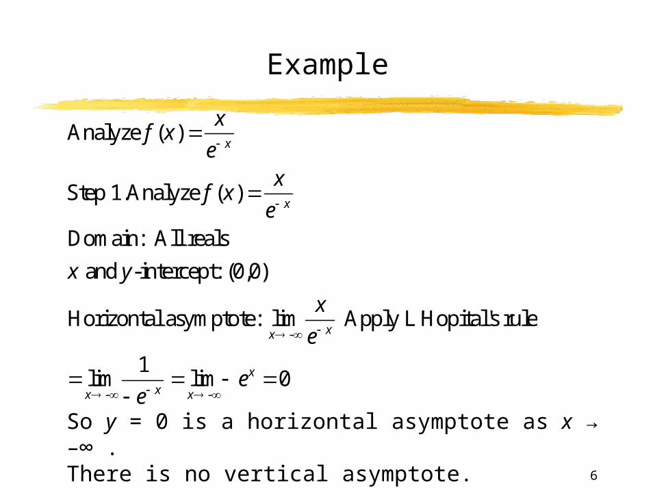
So y = 0 is a horizontal asymptote as x → –∞ .There is no vertical asymptote.
Analyze f (x) x
e x
Step 1.Analyze f (x) x
e x
Domain: All reals
x and y-intercept: (0,0)
Horizontal asymptote: limx -
x
e x Apply L'Hopital's rule
limx -
1
e x lim
x - ex 0
7
Example(continued)
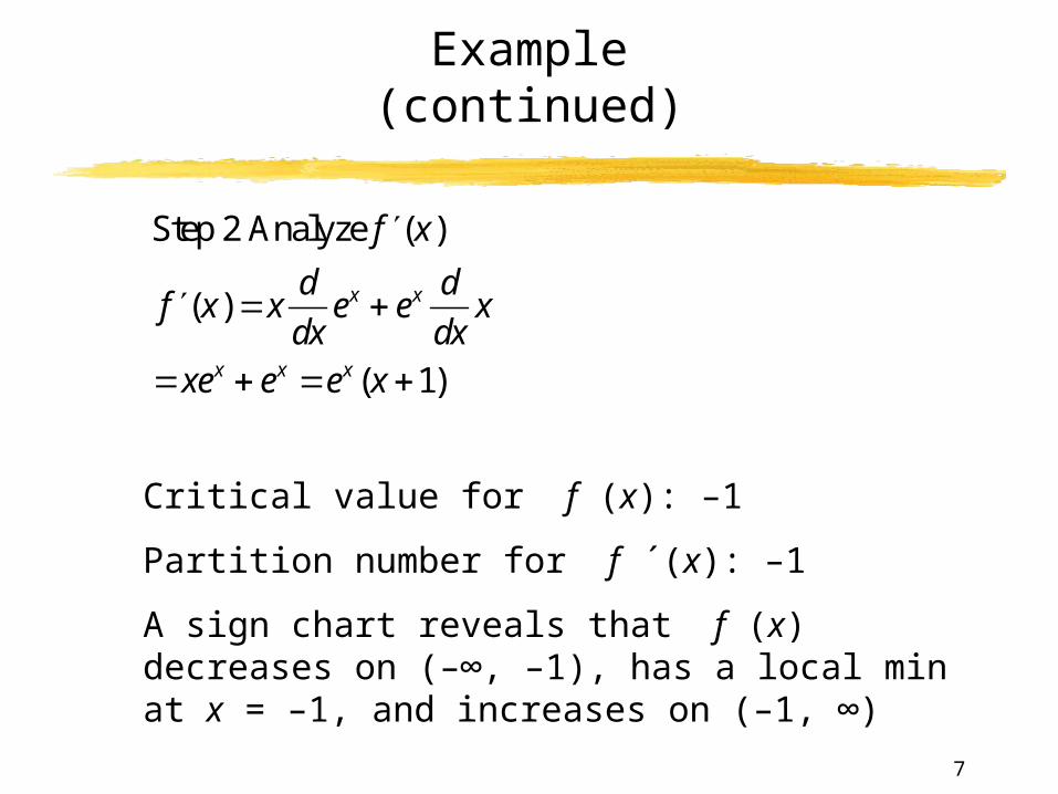
Critical value for f (x): –1
Partition number for f ´(x): –1
A sign chart reveals that f (x) decreases on (–∞, –1), has a local min at x = –1, and increases on (–1, ∞)
Step 2 Analyze f (x)
f (x) xd
dxex ex d
dxx
xex ex ex (x 1)
8
Example (continued)
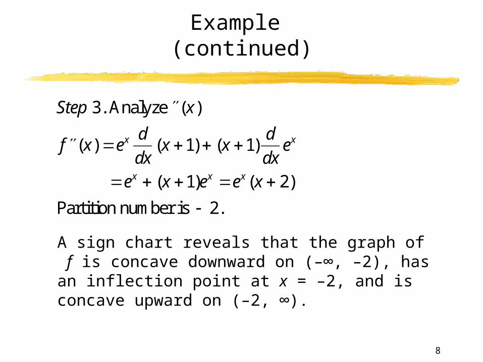
Step 3. Analyze (x)
f (x) ex d
dx(x 1) (x 1)
d
dxex
ex (x 1)ex ex (x 2)
Partition number is 2.
A sign chart reveals that the graph of f is concave downward on (–∞, –2), has an inflection point at x = –2, and is concave upward on (–2, ∞).
9
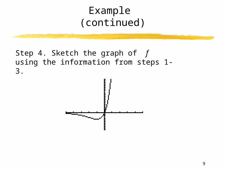
Example (continued)
Step 4. Sketch the graph of f using the information from steps 1-3.
10
Application Example
If x CD players are produced in one day, the cost per day is
C (x) = x2 + 2x + 2000
and the average cost per unit is C(x) / x.
Use the graphing strategy to analyze the average cost function.
11
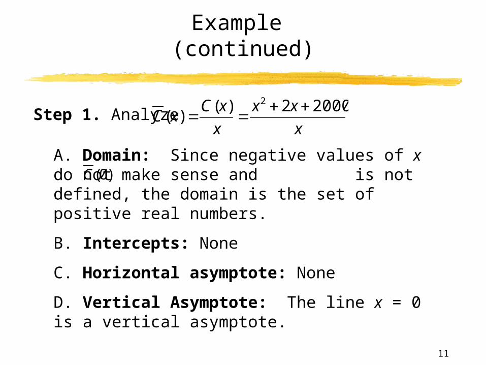
A. Domain: Since negative values of x do not make sense and is not defined, the domain is the set of positive real numbers.
B. Intercepts: None
C. Horizontal asymptote: None
D. Vertical Asymptote: The line x = 0 is a vertical asymptote.
Example (continued)
Step 1. Analyze
(0)C
x
xx
x
xCxC
20002)()(
2
12
Example (continued)
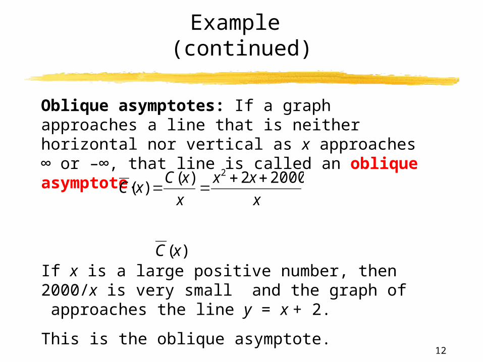
Oblique asymptotes: If a graph approaches a line that is neither horizontal nor vertical as x approaches ∞ or –∞, that line is called an oblique asymptote.
If x is a large positive number, then 2000/x is very small and the graph of approaches the line y = x + 2.
This is the oblique asymptote.
( )C x
x
xx
x
xCxC
20002)()(
2
13
C (x)
x(2x 2) (x2 2x 2000)
x2
x2 2000
x2
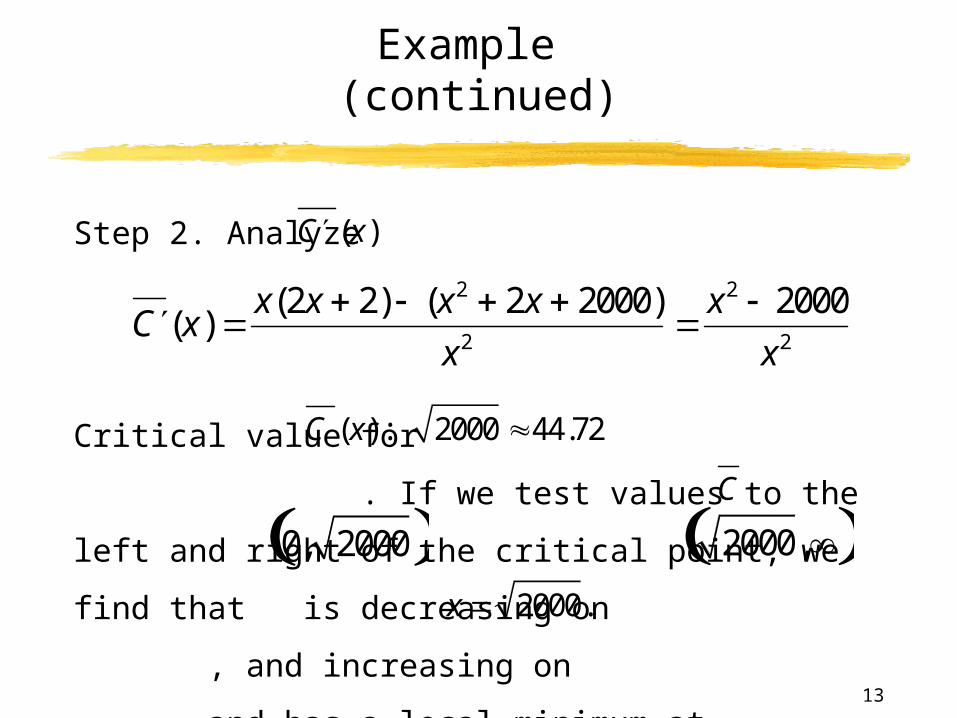
Critical value for . If we test values to
the left and right of the critical point, we find that is
decreasing on , and increasing on
and has a local minimum at
Example (continued)
Step 2. Analyze
2000,
C (x) : 2000 44.72
0, 2000
C
x 2000.
C (x)
14
Example (continued)
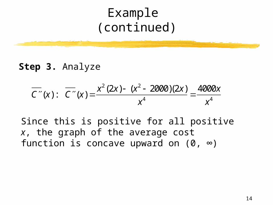
Step 3. Analyze
Since this is positive for all positive x, the graph of the average cost function is concave upward on (0, ∞)
C (x) : C (x)
x2(2x) (x2 2000)(2x)
x4
4000x
x4
15
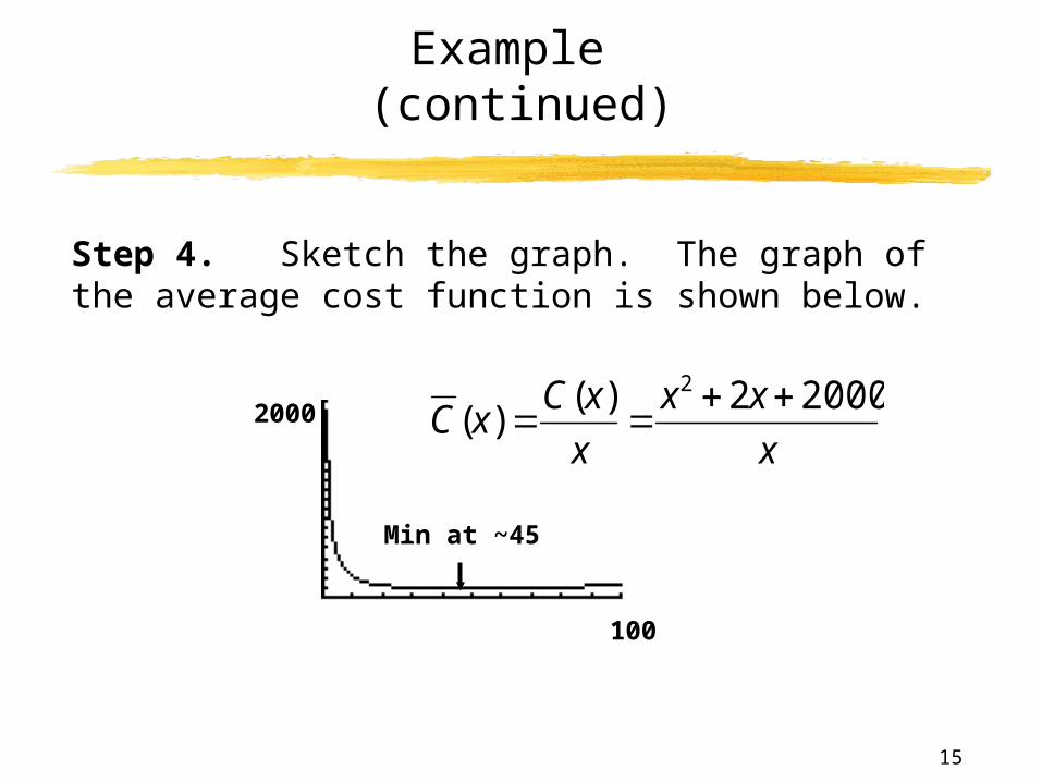
Example (continued)
Step 4. Sketch the graph. The graph of the average cost function is shown below.
2000
100
Min at ~45
x
xx
x
xCxC
20002)()(
2
16
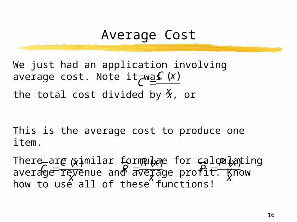
We just had an application involving average cost. Note it was
the total cost divided by x, or
This is the average cost to produce one item.
There are similar formulae for calculating average revenue and average profit. Know how to use all of these functions!
x
xCC
)(
x
xCC
)(
x
xRR
)(
x
xPP
)(
Average Cost