Embed Size (px)
Citation preview
Chapter 5
Modelling the formation of doublewhite dwarfs
M.V. van der Sluys, F. Verbunt and O.R. Pols
Submitted to Astronomy and Astrophysics
Abstract We investigate the formation of the ten double-lined doublewhite dwarfs thathave been observed so far. A detailed stellar evolution codeis used to calculate grids ofsingle-star and binary models and we use these to reconstruct possible evolutionary sce-narios. We apply various criteria to select the acceptable solutions from these scenarios.We confirm the conclusion ofNelemans et al.(2000) that formation via conservative masstransfer and a common envelope with spiral-in based on energy balance or via two suchspiral-ins cannot explain the formation of all observed systems. We investigate three differ-ent prescriptions of envelope ejection due to dynamical mass loss with angular-momentumbalance and show that they can explain the observed masses and orbital periods well. Next,we demand that the age difference of our model is comparable to the observed cooling-age difference and show that this puts a strong constraint onthe model solutions. One ofthese solutions explains the DB-nature of the oldest white dwarf in PG 1115+116 along theevolutionary scenario proposed byMaxted et al.(2002a), in which the helium core of theprimary becomes exposed due to envelope ejection, evolves into a giant phase and loses itshydrogen-rich outer layers.

80 Chapter 5
5.1 Introduction
Ten double-lined spectroscopic binaries with two white-dwarf components are currentlyknown. These binaries have been systematically searched for to find possible progenitorsystems for Type Ia supernovae, for instance by the SPY (ESO SN Ia Progenitor surveY)project (e.g. Napiwotzki et al. 2001, 2002). Short-period double white dwarfs can loseorbital angular momentum by emitting gravitational radiation and if the total mass of thebinary exceeds the Chandrasekhar limit, their eventual merger might produce a supernovaof type Ia (Iben & Tutukov 1984).
The observed binary systems all have short orbital periods that, with one exception,range from an hour and a half to a day or two (see Table5.1), corresponding to orbital sep-arations between 0.6R⊙ and 7R⊙. The white-dwarf masses of 0.3M⊙ or more indicatethat their progenitors were (sub)giants with radii of a few tens to a few hundred solar radii.This makes a significant orbital shrinkage (spiral-in) during the last mass-transfer phasenecessary and fixes the mechanism for the last mass transfer to common-envelope evolu-tion. In such an event the envelope of the secondary engulfs the oldest white dwarf due todynamically-unstable mass transfer. Friction then causesthe two white dwarfs to spiral intowards each other while the envelope is expelled. The orbital energy that is freed due tothe spiral-in provides for the necessary energy for the expulsion (Webbink 1984).
The first mass transfer phase is usually thought to be either another spiral-in or stableand conservative mass transfer. The first scenario predictsthat the orbit shrinks appreciablyduring the mass transfer whereas the second suggests a widening orbit. Combined witha core mass–radius relation (e.g. Refsdal & Weigert 1970) these scenarios suggest thatthe mass ratioq2 ≡ M2/M1 of the double white dwarfs is much smaller than unity inthe first scenario and larger than unity in the second scenario. The observed systems allhave mass ratios between 0.70 and 1.28 (Table5.1), which ledNelemans et al.(2000) toconclude that a third mechanism is necessary to explain the evolution of these systems.They suggested envelope ejection due to dynamical mass lossbased on angular-momentumbalance, in which little orbital shrinkage takes place. They used analytical approximationsto reconstruct the evolution of three double white dwarfs and concluded that these threesystems can only be modelled if this angular-momentum prescription is included.
In this chapter we will use the same method asNelemans et al.(2000), to see if astable-mass-transfer episode followed by a common envelope with spiral-in can explain theobserved double white dwarfs. We will improve on their calculations in several respects.First, we extend the set of observed binaries from 3 to 10 systems. Second, we take intoaccount progenitor masses for the white dwarf that was formed last up to10 M⊙ and allowthem to evolve beyond core helium burning to the asymptotic giant branch.Nelemans et al.(2000) restricted themselves to progenitor masses of2.3 M⊙ or less and did not allow thesestars to evolve past the helium flash. This was justified because the maximum white-dwarfmass that should be created by these progenitors was0.47 M⊙, the maximum helium-coremass of a low-mass star and less than the minimum mass for a CO white dwarf formed in aspiral-in (see Fig.5.1). The most massive white dwarf in our sample is0.71 M⊙ and cannot
Modelling the formation of double white dwarfs 81
have been created by a low-mass star on the red-giant branch.Third, we use more sophis-ticated stellar models to reconstruct the evolution of the observed systems. This means thatthe radius of our model stars does not depend on the helium-core mass only, but also ontotal mass of the star (see Fig.5.1). Furthermore, we can calculate the binding energy of thehydrogen envelope of our models so that we do not need the envelope-structure parameterλenv and can calculate the common-envelope parameterαce directly. Last, because we usea full binary-evolution code, we can accurately model the stable mass transfer rather thanestimate the upper limit for the orbital period after such a mass-transfer phase. This placesa strong constraint on the possible stable-mass-transfer solutions. The evolution code alsotakes into account the fact that the core mass of a donor star can grow appreciably duringstable mass transfer, a fact that alters the relation between the white-dwarf mass and theradius of the progenitor mentioned earlier for the case of stable mass transfer.
Our research follows the lines ofNelemans et al.(2000), calculating the evolution of thesystems in reverse order, from double white dwarf, via some intermediate system with onewhite dwarf, to the initial ZAMS binary. In Sect.5.2we list the observed systems that we tryto model. The stellar evolution code that we use to calculatestellar models is described inSect.5.3. In Sect.5.4we present several grids of single-star models from which wewill usethe helium-core mass, stellar radius and envelope binding energy to calculate the evolutionduring a spiral-in. We show a grid of ‘basic’ models with standard parameters and describethe effect of chemical enrichment due to accretion and the wind mass loss. We find that thesetwo effects may be neglected for our purpose. In Sect.5.5we use the single-star models tocalculate spiral-in evolution for each observed binary andeach model star in our grid andthus produce a set of progenitor binaries. Many of these systems can be rejected based onthe values for the common-envelope parameter or orbital period. The remainder is a seriesof binaries consisting of a white dwarf and a giant star that would cause a common envelopewith spiral-in and produce one of the observed double white dwarfs. In Sect.5.6we modelthe first mass-transfer scenario that produces the systems found in Sect.5.5to complete theevolution. We consider three possible mechanisms: stable and conservative mass transfer,a common envelope with spiral-in based on energy balance andenvelope ejection based onangular-momentum balance. We introduce two variations in the latter mechanism and showthat they can explain the observed binaries. In addition, weshow that the envelope-ejectionscenario based on angular-momentum balance can also explain the second mass-transferepisode. In Sect.5.6.4we include the observed age difference in the list of parameters ourmodels should explain and find that this places a strong constraint on our selection criteria.In Sect.5.7 we compare this study to earlier work and discuss an alternative formationscenario for PG 1115+116. Our conclusions are summed up in Sect.5.8.
5.2 Observed double white dwarfs
At present, ten double-lined spectroscopic binaries consisting of two white dwarfs havebeen observed. The orbital periods of these systems are welldetermined. The fact that bothcomponents are detected makes it possible to constrain the mass ratio of the system from

82 Chapter 5
the radial-velocity amplitudes. The masses of the components are usually determined byfitting white-dwarf atmosphere models to the observed effective temperature and surfacegravity, using mass–radius relations for white dwarfs. Thevalues thus obtained are clearlybetter for the brightest white dwarf but less well-constrained than the values for the periodor mass ratio. It is also harder to estimate the errors on the derived mass. In the publicationsof these observations, the brightest white dwarf is usuallydenoted as ‘star 1’ or ‘star A’.Age determinations suggest in most cases that the brightestcomponent of these systemsis the youngest white dwarf. These systems must have evolvedthrough two mass-transferepisodes and the brightest white dwarf is likely to have formed from the originally lessmassive component of the initial binary (consisting of two ZAMS stars). We will call thisstar the secondary or ‘star 2’ throughout this chapter, whereas the primary or ‘star 1’ is thecomponent that was the initially more massive star in the binary. The two components willcarry these labels throughout their evolution, and therefore white dwarf 1 will be the oldestand usually the faintest and coldest of the two observed components. The properties of theten double-lined white-dwarf systems are listed in Table5.1. For our calculations we willuse the parameters that are best determined from the Table:Porb, q2 andM2. For M1 wewill notuse the value listed in Table5.1, but the valueM2/q2 instead. We hereby ignore theobservational uncertainties inq2, because they are small with respect to the uncertainties inthe mass. In Sects.5.5and5.6we will use a typical value of0.05 M⊙ (Maxted et al. 2002b)for the uncertainties in the estimate of the secondary mass.
Although the cooling-age determinations are strongly dependent on the cooling modelused, the thickness of the hydrogen layer on the surface and the occurrence of shell flashes,the cooling-agedifferenceis thought to suffer less from systematic errors. The valuesfor ∆τin Table5.1have an estimated uncertainty of 50% (Maxted et al. 2002b). The age determina-tions of the components of WD 1704+481a suggest that star 2 may be the oldest white dwarf,although the age difference is small in both absolute (20 Myr) and relative (≈3%) sense(Maxted et al. 2002b). Because of this uncertainty we will introduce an eleventhsystemwith a reversed mass ratio. This new system will be referred to as WD 1704+481b or 1704band since we assume that the value forM2 is better determined, we will use the followingvalues for this system:M1 = 0.39 M⊙, q2 = 1.43 ± 0.06 andM2 ≡ q2M1 = 0.56 M⊙.
5.3 The stellar evolution code
We calculate our models using the STARS binary stellar evolution code, originally devel-oped byEggleton(1971, 1972) and with updated input physics as described inPols et al.(1995). Opacity tables are taken from OPAL (Iglesias et al. 1992), complemented withlow-temperature opacities fromAlexander & Ferguson(1994).
The equations for stellar structure and composition are solved implicitly and simulta-neously, along with an adaptive mesh-spacing equation. Because of this, the code is quitestable numerically and relatively large timesteps can be taken. As a result of the largetimesteps and because hydrostatic equilibrium is assumed,the code does not easily pick upshort-time-scale instabilities such as thermal pulses. Wecan thus quickly evolve our models
Modelling
theform
ationofdouble
white
dwarfs
83
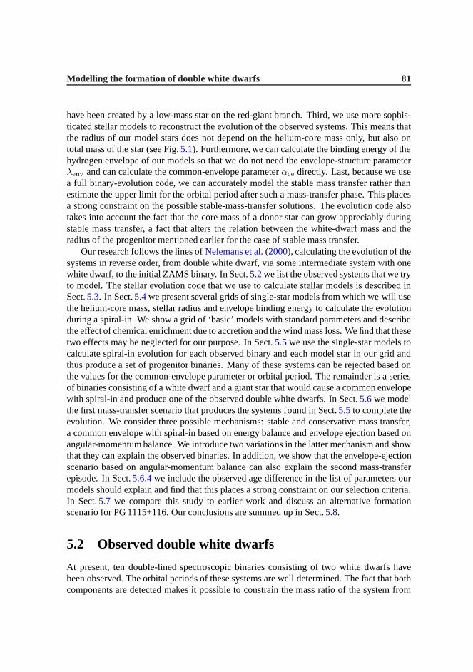
Name Porb (d) aorb (R⊙) M1 (M⊙) M2 (M⊙) q2 = M2/M1 τ2 (Myr) ∆τ (Myr) Ref/NoteWD 0135–052 1.556 5.63 0.52± 0.05 0.47± 0.05 0.90± 0.04 950 350 1,2WD 0136+768 1.407 4.98 0.37 0.47 1.26± 0.03 150 450 3,10WD 0957–666 0.061 0.58 0.32 0.37 1.13± 0.02 25 325 3,5,6,10WD 1101+364 0.145 0.99 0.33 0.29 0.87± 0.03 135 215 4,(10)PG 1115+116 30.09 40.0 0.7 0.7 0.84± 0.21 60 160 8,9
WD 1204+450 1.603 5.72 0.52 0.46 0.87± 0.03 40 80 6,10WD 1349+144 2.209 6.65 0.44 0.44 1.26± 0.05 — — 12HE 1414–0848 0.518 2.93 0.55± 0.03 0.71± 0.03 1.28± 0.03 1000 200 11WD 1704+481a 0.145 1.13 0.56± 0.07 0.39± 0.05 0.70± 0.03 725 -20 7,aHE 2209–1444 0.277 1.89 0.58± 0.08 0.58± 0.03 1.00± 0.12 900 500 13
Table 5.1: Observed double white dwarfs discussed in this chapter. The table shows for each system the orbital periodPorb, theorbital separationaorb, the massesM1 andM2, the mass ratioq2 = M2/M1, the estimated cooling age of the youngest whitedwarf τ2 and the difference between the cooling ages of the components∆τ . M1 is the mass of the oldest white dwarf and thuspresumably the original primary. The errors on the periods are smaller than the last digit. The values foraorb are calculated bythe authors and meant to give an indication. References: (1)Saffer et al.(1988), (2) Bergeron et al.(1989), (3) Bragaglia et al.(1990), (4) Marsh(1995), (5) Moran et al.(1997), (6) Moran et al.(1999), (7) Maxted et al.(2000), (8) Bergeron & Liebert(2002), (9) Maxted et al.(2002a), (10)Maxted et al.(2002b), (11)Napiwotzki et al.(2002), (12)Karl et al.(2003a), (13)Karlet al.(2003b). Note: (a) WD 1704+481a is the close pair of a hierarchical triple. It seems unclear which of the two stars in thispair is the youngest (see the text).
84 Chapter 5
up the asymptotic giant branch (AGB), without having to calculate a number of pulses indetail. We thus assume that such a model is a good representation of an AGB star.
Convective mixing is modelled by a diffusion equation for each of the compositionvariables, and we assume a mixing-length to scale-height ratio l/Hp = 2.0. Convectiveovershooting is taken into account as inSchroder et al.(1997), with a parameterδov = 0.12which corresponds to overshooting lengths of about 0.3 pressure scale heights (Hp) and iscalibrated against accurate stellar data from non-interacting binaries (Schroder et al. 1997;Pols et al. 1997). The code circumvents the helium flash in the degenerate core of a low-mass star by replacing the model at which the flash occurs by a model with the same totalmass and core mass but a non-degenerate helium core in which helium was just ignited. Themasses of the helium and carbon-oxygen cores are defined as the mass coordinates wherethe abundances of hydrogen and helium respectively become less than 10%. The bindingenergy of the hydrogen envelope of a model is calculated by integrating the sum of theinternal and gravitational energy over the mass coordinate, from the helium-core massMc
to the surface of the starMs:
Ub,e =
∫ Ms
Mc
(
Uint(m) −Gm
r(m)
)
dm (5.1)
The termUint is the internal energy per unit of mass, that contains terms such as the thermalenergy and recombination energy of hydrogen and helium.
We use a version of the code (seeEggleton & Kiseleva-Eggleton 2002) that allows fornon-conservative binary evolution. We use the code to calculate the evolution of both singlestars and binaries in which both components are calculated in full detail. With the adaptivemesh, mass loss by stellar winds or by Roche-lobe overflow (RLOF) in a binary is simplyaccounted for in the boundary condition for the mass. The spin of the stars is neglected in thecalculations and the spin-orbit interaction by tides is switched off. The initial compositionof our model stars is similar to solar composition:X = 0.70, Y = 0.28 andZ = 0.02.
5.4 Giant branch models
As we have seen in Sect.5.1, each of the double white dwarfs that are observed today musthave formed in a common-envelope event that caused a spiral-in of the two degenerate starsand expelled the envelope of the secondary. The intermediate binary system that existedbefore this event, but after the first mass-transfer episode, consisted of the first white dwarf(formed from the original primary) and a giant-branch star (the secondary). This giant isthus the star that caused the common envelope and in order to determine the properties ofthe spiral-in that formed each of the observed systems, we need a series of giant-branchmodels. In this section we present a grid of models for singlestars that evolve from theZAMS to high up the asymptotic giant branch (AGB). For each time step we saved the totalmass of the star, the radius, the helium-core mass and the binding energy of the hydrogenenvelope of the star.
Modelling the formation of double white dwarfs 85
In an attempt to cover all possibilities, we need to take intoaccount the effects thatcan change the quantities mentioned above. We consider the chemical enrichment of thesecondary by accretion in a first mass-transfer phase and theeffect a stellar-wind mass lossmay have. For each of these changes, we compare the results toa grid of ‘basic’ modelswith default parameters. We keep the overshooting parameter δov constant for all thesegrids, because this effect is unimportant for low-mass stars (M ∼< 2.0 M⊙) and its value iswell calibrated for intermediate-mass stars (see Sect.5.3).
5.4.1 Basic models
In order to find the influence of the effects mentioned above, we want to compare the modelsincluding these effects to a standard. We therefore calculated a grid of stellar models, fromthe zero-age main sequence to high up the asymptotic giant branch (AGB), with defaultvalues for all parameters. These models have solar composition and no wind mass loss.We calculated a grid of199 single-star models with these parameters with masses between0.80 and 10.0M⊙, with the logarithm of their masses evenly distributed. Model stars withmasses lower than about 2.05M⊙ experience a degenerate core helium flash and are at thatpoint replaced by a post-helium-flash model as described in Sect.5.3. Because of the largetimesteps the code can take, the models evolve beyond the point on the AGB where thecarbon-oxygen core (CO-core) mass has caught up with the helium-core mass and the firstthermal pulse should occur.
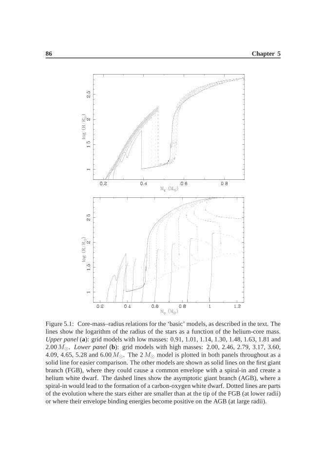
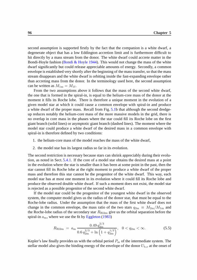
Figure5.1shows the radii of a selection of our grid models as a functionof their helium-core masses. We used different line styles to mark differentphases in the evolution of thesestars, depending on their ability to fill their Roche lobes orcause a spiral-in and the typeof star a common envelope would result in. The solid lines show the evolution up the firstgiant branch (FGB), where especially the low-mass stars expand much and could cause acommon envelope with spiral-in, in which a helium white dwarf would be formed. Fig.5.1ashows that low-mass stars briefly contract for core masses around 0.3M⊙. This is due tothe first dredge-up, where the convective envelope deepens down to just above the hydrogenburning shell and increases the hydrogen abundance there. The contraction happens whenthe hydrogen-burning shell catches up with this composition discontinuity. After ignitionof helium in the core, all stars shrink and during core heliumburning and the first phaseof helium fusion in a shell, their radii are smaller than at the tip of the FGB. This meansthat these stars could never start filling their Roche lobes in this stage. These parts of theevolution are plotted with dotted lines. Once a CO core is established, the stars evolve upthe AGB and eventually get a radius that is larger than that onthe FGB. The stars are nowcapable of filling their Roche lobes again and cause a common envelope with spiral-in. Insuch a case we assume that the whole helium core survives the spiral-in and that the heliumburning shell will convert most of the helium to carbon and oxygen, eventually resultingin a CO white dwarf, probably with an atmosphere that consists of a mixture of hydrogenand helium. This part of the evolution is marked with dashed lines. Fig.5.1b shows thatthe most massive models in our grid have a decreasing helium-core mass at some point
86 Chapter 5
Figure 5.1: Core-mass–radius relations for the ‘basic’ models, as described in the text. Thelines show the logarithm of the radius of the stars as a function of the helium-core mass.Upper panel(a): grid models with low masses: 0.91, 1.01, 1.14, 1.30, 1.48,1.63, 1.81 and2.00M⊙. Lower panel(b): grid models with high masses: 2.00, 2.46, 2.79, 3.17, 3.60,4.09, 4.65, 5.28 and 6.00M⊙. The 2M⊙ model is plotted in both panels throughout as asolid line for easier comparison. The other models are shownas solid lines on the first giantbranch (FGB), where they could cause a common envelope with aspiral-in and create ahelium white dwarf. The dashed lines show the asymptotic giant branch (AGB), where aspiral-in would lead to the formation of a carbon-oxygen white dwarf. Dotted lines are partsof the evolution where the stars either are smaller than at the tip of the FGB (at lower radii)or where their envelope binding energies become positive onthe AGB (at large radii).

Modelling the formation of double white dwarfs 87
on the AGB. This happens at the so-called second dredge-up, where the convective mantleextends inward, into the helium core and mixes some of the helium from the core into themantle, thereby reducing the mass of the core. Models with masses between about 1.2and 5.6M⊙ expand to such large radii that the binding energy of their hydrogen envelopesbecome positive. In Sect.5.5we are looking for models that can cause a spiral-in based onenergy balance in the second mass-transfer phase, for whichpurpose we require stars thathave hydrogen envelopes with a negative binding energy. A positive binding energy meansthat there is no orbital energy needed for the expulsion of the envelope and thus the orbitwill not shrink during a common envelope caused by such a star. We have hereby implicitlyassumed that the recombination energy is available during common-envelope ejection.
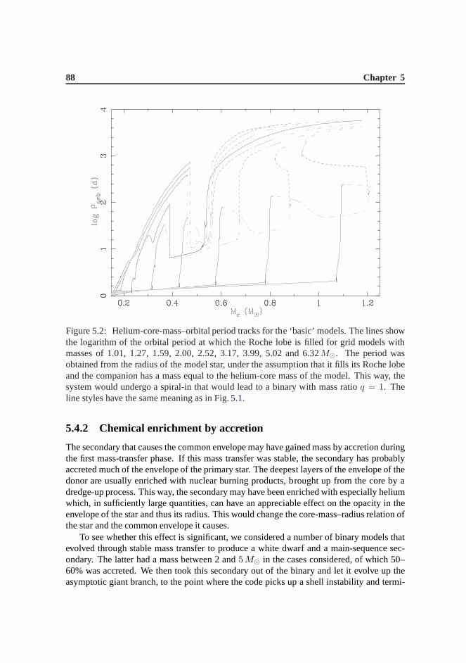
To give some idea what kind of binaries can cause a spiral-in and could be the progen-itors of the observed double white dwarfs, we converted the radii of the stars displayed inFig.5.1 into orbital periods of the pre-common-envelope systems. To do this, we assumedthat the Roche-lobe radius is equal to the radius of the modelstar, and that the mass of thecompanion is equal to the mass of the helium core of the model.This is justified by Ta-ble5.1, where the geometric mean of the mass ratios is equal to 1.03.The result is shownin Fig.5.2.
In Sect.5.5we will need the efficiency parameterαce of each common-envelope modelto judge whether that model is acceptable or not. In order to calculate this parameter wemust know the binding energy of the hydrogen envelope of the progenitor star (see Eq.5.4),that is provided by the evolution code as shown in Eq.5.1. The envelope binding energy istherefore an important parameter and we show it for a selection of models in Fig.5.3, againas a function of the helium-core mass. Because the binding energy is usually negative, weplot the logarithm of−Ub,e. The phases where the envelope binding energy is non-negativeare irrelevant for our calculations ofαce and therefore not shown in the Figure.
Many common-envelope calculations in the literature use the so-called envelope-structure parameterλenv to estimate the envelope binding energy from basic stellar pa-rameters in case a detailed model is not available
Ub,e = −GM∗ Menv
λenv R∗
. (5.2)
De Kool et al.(1987) suggest thatλenv ≈ 0.5. Since we calculate the binding energy ofthe stellar envelope accurately, we can invert Eq.5.2 and calculateλenv (see alsoDewi &Tauris 2000). Figure5.4shows the results of these calculations as a function of the heliumcore mass, for the same selection of models as in Fig.5.3. We see that a value ofλenv = 0.5is a good approximation for the lower FGB of a low-mass star, or the FGB of a higher-massstar. A low-mass star near the tip of the first giant branch hasa structure parameter between0.5 and 1.5 and for most starsλenv increases to more than unity rather quickly, especiallywhen the stars expand to large radii and the binding energiescome close to zero.
88 Chapter 5
Figure 5.2: Helium-core-mass–orbital period tracks for the ‘basic’ models. The lines showthe logarithm of the orbital period at which the Roche lobe isfilled for grid models withmasses of 1.01, 1.27, 1.59, 2.00, 2.52, 3.17, 3.99, 5.02 and 6.32M⊙. The period wasobtained from the radius of the model star, under the assumption that it fills its Roche lobeand the companion has a mass equal to the helium-core mass of the model. This way, thesystem would undergo a spiral-in that would lead to a binary with mass ratioq = 1. Theline styles have the same meaning as in Fig.5.1.
5.4.2 Chemical enrichment by accretion
The secondary that causes the common envelope may have gained mass by accretion duringthe first mass-transfer phase. If this mass transfer was stable, the secondary has probablyaccreted much of the envelope of the primary star. The deepest layers of the envelope of thedonor are usually enriched with nuclear burning products, brought up from the core by adredge-up process. This way, the secondary may have been enriched with especially heliumwhich, in sufficiently large quantities, can have an appreciable effect on the opacity in theenvelope of the star and thus its radius. This would change the core-mass–radius relation ofthe star and the common envelope it causes.
To see whether this effect is significant, we considered a number of binary models thatevolved through stable mass transfer to produce a white dwarf and a main-sequence sec-ondary. The latter had a mass between 2 and5 M⊙ in the cases considered, of which 50–60% was accreted. We then took this secondary out of the binary and let it evolve up theasymptotic giant branch, to the point where the code picks upa shell instability and termi-

Modelling the formation of double white dwarfs 89
Figure 5.3: The logarithm of the binding energy of the ‘basic’ model stars as a functionof the helium-core mass. The grid models with masses of 0.91,1.01, 1.14, 1.30, 1.48,1.63, 1.81, 2.00, 2.46, 2.79, 3.17, 3.70, 4.09, 4.65, 5.28, 6.00 and 6.82M⊙ are shown. The2.00M⊙ model is drawn as a solid line, the line styles for the other models have the samemeaning as in Fig.5.1. The parts where the envelope binding energy is zero (beforea heliumcore develops) or positive are not shown.
nates. We then compared this final model to a model of a single star with the same mass, butwith solar composition, that was evolved to the same stage. In all cases the core mass–radiusrelations coincide with those in Fig.5.1. When we compared the surface helium abundancesof these models, after one or two dredge-ups, we found that although the abundances wereenhanced appreciably since the ZAMS, they were enhanced with approximately the sameamount and the relative difference of the helium abundance at the surface between the dif-ferent models was always less than 1.5%. In some cases the model that had accreted from acompanion had the lower surface helium abundance.
The small amount of helium enrichment due to accretion givesrise to such small changesin the core mass–radius relation, that we conclude that thiseffect can be ignored in ourcommon-envelope calculations in Sect.5.5.

90 Chapter 5
Figure 5.4: The envelope-structure parameterλenv for the ‘basic’ models, as a function ofthe helium-core mass. The same grid models are shown as in Fig.5.3. The meaning of theline styles is explained in the caption of Fig.5.1.
5.4.3 Wind mass loss
The mass loss of a star by stellar wind can change the mass of a star appreciably beforethe onset of Roche-lobe overflow, and the mass loss can influence the relation betweenthe core mass and the radius of a star. From Fig.5.1 it is already clear that this relationdepends on the total mass of the star. In this section, we would therefore like to find outwhether a conservative model star of a certain total mass andcore mass has the same radiusand envelope binding energy as a model with the same total mass and core mass, but thatstarted out as a more massive star, has a strong stellar wind and just passes by this masson its evolution down to even lower masses. We calculated a small grid of models with tendifferent initial masses between 1.0M⊙ and 8.0 M⊙, evenly spread inlog M and includeda Reimers type mass loss (Reimers 1975) of variable strength:
Mrml = −4 × 10⁻¹³ M⊙ yr−1 Crml
(
L
L⊙
) (
R
R⊙
)(
M
M⊙
)−1
, (5.3)
where we have used the valuesCrml = 0.2, 0.5 and 1.0. The basic models of Sect.5.4.1areconservative and therefore haveCrml = 0. The effect of these winds on the total mass of themodel stars in our grid is displayed in Fig.5.5. It shows the fraction of mass lost at the tipof the first giant branch (FGB) and the ‘tip of the asymptotic giant branch’ (AGB). The first

Modelling the formation of double white dwarfs 91
Figure 5.5: The fraction of mass lost at two moments in the evolution of a star as a functionof its initial mass, for the three different wind strengths (Crml = 0.2, 0.5 and 1.0) used in thegrid. This fraction is shown for the tip of the FGB (dashed lines and crosses), and the ‘tipof the AGB’ (dotted lines and plusses). See the text for details.
moment is defined as the point where the star reaches its largest radius before helium ignitesin the core, the second as the point where the radius of the star reaches its maximum valuewhile the envelope binding energy is still negative. Valuesfor both moments are plotted inFig.5.5 for each non-zero value ofCrml in the grid. For the two models with the lowestmasses the highest mass-loss rates are so high that the totalmass is reduced sufficiently onthe FGB to keep the star from igniting helium in the core, and the lines in the plot coincide.Stars more massive than 2M⊙ have negligible mass loss on the FGB, because they havenon-degenerate helium cores so that they do not ascend the FGB as far as stars of lowermass. Their radii and luminosities stay relatively small, so that Eq.5.3 gives a low massloss rate. For stars of 4M⊙ or more, the mass loss is diminutive and happens only shortlybefore the envelope binding energy becomes positive. We canconclude that for these starsthe wind mass loss has little effect on the core mass–radius relation.
The core mass–radius relations for a selection of the modelsfrom our wind grid areshown in Fig.5.6. The Figure compares models without stellar wind with models that havethe strongest stellar wind in our grid (Crml = 1.0). Models with the other wind strengthswould lie between those shown, but are not plotted for clarity. The greatest difference inFig.5.6 is in the 1.0M⊙ model. The heavy mass loss reduces the total mass of the star to

92 Chapter 5
Figure 5.6: Comparison of a selection from the small grid of models with a stellar wind.The models displayed have masses of 1.0, 1.6, 2.5, 3.2, 4.0, 5.0 and 6.3M⊙. The windstrength parameters areCrml = 0.0 (dotted lines) andCrml = 1.0 (solid lines, the strongestmass loss in the grid). Stars with mass loss are usually larger, but for models of 4.0M⊙ ormore this effect becomes negligible. The 1.0M⊙ model loses so much mass that it neverignites helium in the core.
0.49M⊙ on the first giant branch, so that the star is not massive enough to ignite helium inthe core. Fig.5.6shows that models with mass loss are larger than conservative models forthe same core mass, as one would expect from Fig.5.1. This becomes clear on the FGB forstars that have degenerate helium cores, because they have large radii and luminosities andlose large amounts of mass there. For stars more massive thanabout2 M⊙ the mass lossbecomes noticeable on the AGB. Stars of4 M⊙ or more show little difference in Fig.5.6.The envelope binding energies have similar differences in the same mass regions.
The question is whether the properties of the model with reduced mass due to the windare the same as those for a conservative model of that mass. Inorder to answer this question,we have compared the models from the ‘wind grid’ to the basic,conservative models. Asthe wind reduces the total mass of a model star, it usually reaches masses that are equalto that of several models in the conservative grid. As this happens, we interpolate linearlywithin the mass-losing model to find the exact moment where its mass equals the mass ofthe conservative model. We then use the helium-core mass of the interpolated mass-losingmodel to find the moment where the conservative model has the same core mass and we
Modelling the formation of double white dwarfs 93
calculate its radius and envelope binding energy, again by linear interpolation. This waywe can compare the two models at the moment in evolution wherethey have the same totalmass and the same core mass. This comparison is done in Fig.5.7. Figure5.7a directlycompares the radii of the two sets of models, in Fig.5.7b the ratio of the two radii is shown.
Of the data points in Fig.5.7b 83% lie between 0.9 and 1.1 and 61% between 0.95 and1.05. For the wind models withCrml = 0.2 these numbers are 99% and 97%, and forthe models withCrml = 0.5 they are 94% and 85% respectively. As can be expected, themodels that have a lower — and perhaps a more realistic — mass-loss rate compare betterto the conservative models. We see in Fig.5.7a that many of the points that lie farther fromunity need only a small shift in core mass to give a perfect match. This shift is certainly lessthan0.05 M⊙, which is what we will adopt for the uncertainty of the white-dwarf masses inSect.5.5. We conclude here that there is sufficient agreement betweena model that reachesa certain total mass because it suffers from mass loss and a conservative model of the samemass. The agreement is particularly good for stars high up onthe FGB or AGB, where thedensity contrast between core and envelope is very large.
5.5 Second mass-transfer phase
For the formation of two white dwarfs in a close binary system, two phases of mass transfermust happen. We will call the binary system before the first mass transfer theinitial binary,with masses and orbital periodM1i, M2i andPi. If one considers mass loss due to stellarwind before the first mass-transfer episode, these parameters are not necessarily equal to theZAMS parameters, especially for large ‘initial’ periods. The binary between the two mass-transfer phases is referred to as theintermediate binarywith M1m, M2m andPm. Afterthe two mass-transfer episodes, we obtain thefinal binarywith parametersM1f , M2f andPf , that should correspond to the values that are now observed and listed in Table5.1. Thesubscripts ‘1’ and ‘2’ are used for the initial primary and secondary as defined in Sect.5.2.
In the first mass transfer, the primary star fills its Roche lobe and loses mass, that mayor may not be accreted by the secondary. This leads to the formation of the intermediatebinary, that consists of the first white dwarf and a secondaryof unknown mass. In the secondmass-transfer phase, the secondary fills its Roche lobe and loses its envelope. The secondmass transfer results in the observed double white dwarf binaries that are listed in Table5.1and must account for significant orbital shrinkage. This is because the youngest white dwarfmust have been the core of its progenitor, the secondary in the intermediate binary. Starswith cores between 0.3 and 0.7M⊙ usually have radii of several tens to several hundredsof solar radii, and the orbital separation of the binaries they reside in must be even largerthan that. The orbital separation of the observed systems istypically only in the order of afew solar radii (Table5.1). Giant stars with large radii have deep convective envelopes andwhen such a star fills its Roche lobe, the ensuing mass transfer will be unstable and occuron a very short, dynamical timescale, especially if the donor is much more massive than itscompanion. It is thought that the envelope of such a star can engulf its companion and thisevent is referred to as acommon envelope. The companion and the core of the donor orbit

94 Chapter 5
Figure 5.7: Comparison of a selection of grid models withCrml =1.0 with initial masses of1.3, 1.6, 2.0, 2.5 and 3.2M⊙ to the basic models (Crml =0.0). Upper panel(a): Comparisonof the radius of the models with a stellar wind (solid lines) and the radius of a basic modelwith the same mass and core mass (plusses).Lower panel(b): The fraction of the radius ofthe wind modelRw over the radius of the basic modelRb with the same total and core mass.Each data point corresponds to a point in the upper panel. Of the data points in the upperpanel, 7 out of 143 (5%) lie outside the plot boundaries in thelower panel. The dashed linesshow the region where agreement is better than 10%, where 83%of the data points lie. The1.0M⊙ model was left out because there are only a few basic models with lower mass, thehigher-mass models were left out because they lose very little mass (see Fig.5.5).
Modelling the formation of double white dwarfs 95
inside the common envelope and drag forces will release energy from the orbit, causing theorbit to shrink and the two degenerate stars to spiral in. Thefreed orbital energy will heatthe envelope and eventually expel it. This way, the hypothesis of the common envelopewith spiral-in can phenomenologically explain the formation of close double-white-dwarfbinaries.
5.5.1 The treatment of a spiral-in
In order to estimate the orbital separation of the post-common envelope system quantita-tively, it is often assumed that the orbital energy of the system is decreased by an amountthat is equal to the binding energy of the envelope of the donor star (Webbink 1984):
Ub,e = −αce
[
GM1fM2f
2af
−GM1mM2m
2am
]
. (5.4)
The parameterαce is thecommon-envelopeparameterthat expresses the efficiency by whichthe orbital energy is deposited in the envelope. Intuitively one would expect thatαce ≈ 1.However, part of the liberated orbital energy might be radiated away from the envelopeduring the process, without contributing to its expulsion,thereby loweringαce. Conversely,if the common-envelope phase would last long enough that thedonor star can produce asignificant amount of energy by nuclear fusion, or if energy is released by accretion on tothe white dwarf, this energy will support the expulsion and thus increaseαce.
In the forward calculation of a spiral-in the final orbital separationaf depends stronglyon the parameterαce, which must therefore be known. In this section we will try toestablishthe binary systems that were the possible progenitors of theobserved double white dwarfsand we will therefore performbackwardcalculations. The advantage of this is that we startas close as possible to the observations thus introducing aslittle uncertainty as possible.The problem with this strategy is that we do not know the mass of the secondary progenitorbeforehand. We will have to consider this mass as a free parameter and assume a rangeof possible values for it. The grid of single-star models of Sect.5.4 provides us with thetotal mass, core mass, radius and envelope binding energy atevery moment of evolution,for a range of total masses between 0.8 and 10M⊙. It is then not necessary to know thecommon-envelope parameter, and we can even calculate theαce that is needed to shrink theorbit of a model with a given mass to the observed period of thedouble white dwarf fromthe binding energy. We make two assumptions about the evolution of the two stars duringthe common envelope to perform these backward calculations:
1. the core mass of the donor does not change,
2. the mass of the companion does not change.
The first assumption will be valid if the timescale on which the common envelope takesplace is much shorter than the nuclear-evolution timescaleof the giant donor. This is cer-tainly true, since the mass transfer occurs on the dynamicaltimescale of the donor. The
96 Chapter 5
second assumption is supported firstly by the fact that the companion is a white dwarf, adegenerate object that has a low Eddington accretion limit and is furthermore difficult tohit directly by a mass stream from the donor. The white dwarf could accrete matter in theBondi-Hoyle fashion (Bondi & Hoyle 1944). This would not change the mass of the whitedwarf significantly but could release appreciable amounts of energy. Secondly, a commonenvelope is established very shortly after the beginning ofthe mass transfer, so that the massstream disappears and the white dwarf is orbiting inside thefast-expanding envelope ratherthan accreting mass from the donor. In the terminology used here, the second assumptioncan be written asM1m = M1f .
From the two assumptions above it follows that the mass of thesecond white dwarf,the one that is formed in the spiral-in, is equal to the helium-core mass of the donor at themoment it fills its Roche lobe. There is therefore a unique moment in the evolution of agiven model star at which it could cause a common envelope with spiral-in and producea white dwarf of the proper mass. Recall from Fig.5.1b that although the second dredge-up reduces notably the helium-core mass of the more massive models in the grid, there isno overlap in core mass in the phases where the star could fill its Roche lobe on the firstgiant branch (solid lines) or asymptotic giant branch (dashed lines). The moment where themodel star could produce a white dwarf of the desired mass in acommon envelope withspiral-in is therefore defined by two conditions:
1. the helium-core mass of the model reaches the mass of the white dwarf,
2. the model star has its largest radius so far in its evolution.
The second restriction is necessary because stars can shrink appreciably during their evolu-tion, as noted in Sect.5.4.1. If the core of a model star obtains the desired mass at a pointin the evolution where the star is smaller than it has been at some point in the past, then thestar cannot fill its Roche lobe at the right moment to produce awhite dwarf of the propermass and therefore this star cannot be the progenitor of the white dwarf. This way, eachmodel star has at most one moment in its evolution where it could fill its Roche lobe andproduce the observed double white dwarf. If such a moment does not exist, the model staris rejected as a possible progenitor of the second white dwarf.
If the model star could be the progenitor of the youngest white dwarf in the observedsystem, the computer model gives us the radius of the donor star, that must be equal to theRoche-lobe radius. Under the assumption that the mass of thefirst white dwarf does notchange in the common envelope, the mass ratio of the two starsq2m ≡ M2m/M1m andthe Roche-lobe radius of the secondary starRRl2m give us the orbital separation before thespiral-inam, where we use the fit byEggleton(1983)
RRl2m = am
0.49 q2/3
2m
0.6 q2/32m + ln
(
1 + q1/32m
) , 0 < q2m < ∞. (5.5)
Kepler’s law finally provides us with the orbital periodPm of the intermediate system. Thestellar model also gives the binding energy of the envelope of the donorUb,e at the onset of
Modelling the formation of double white dwarfs 97
the common envelope and we can use Eq.5.4to determine the common-envelope parameterαce. We will useαce to judge the validity of the model star to be the progenitor ofthe secondwhite dwarf. There are several reasons why a numerical solution can be rejected. Firstly, theproposed donor could be a massive star with a relatively small radius. Thenam will be smalland it might happen thatam < af
M2m
M2f, so thatαce < 0. This means that energy is needed
to change the orbit fromam to af , or even thatam < af and a spiral-in (if it can be calledthat) to the desired orbit will not lead to expulsion of the common envelope. Secondly,as mentioned above,αce is expected to be close, though not necessarily equal, to unity.However if the parameter is either much smaller or much larger than 1, we will consider thespiral-in to be ‘physically unbelievable’. We arbitrarilychose the boundaries between whichαce must lie for a believable spiral-in to be a factor of ten either way: 0.1 ≤ αce ≤ 10. Wethink that the actual value forαce should be more constrained than that because common-envelope evolution is thought to last only a short time so that there is little time to generateor radiate large amounts of energy, but keep the range as broad as it is to be certain that allpossible progenitor systems are considered in our sample.
5.5.2 Results of the spiral-in calculations
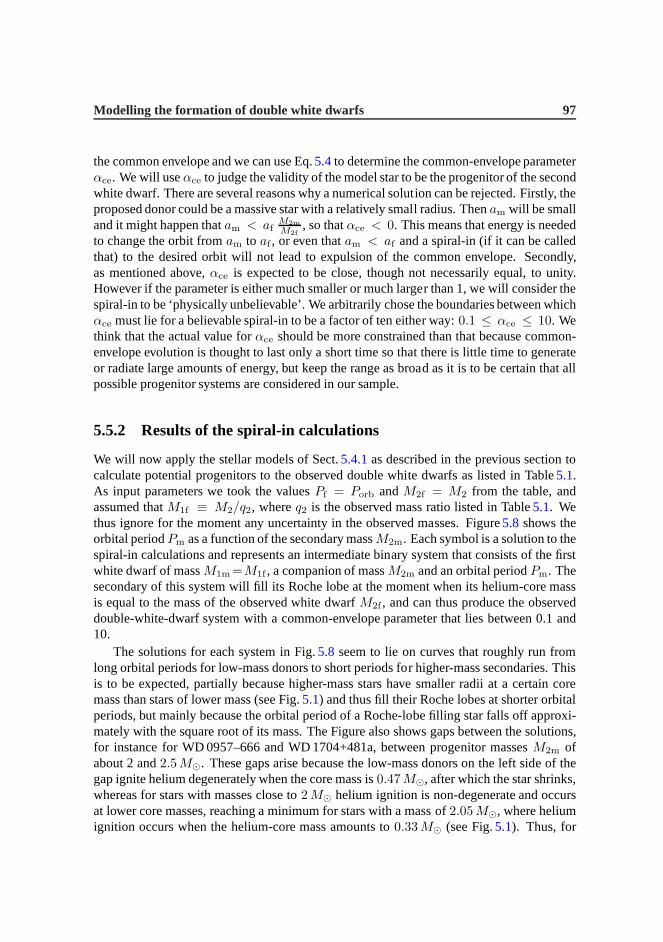
We will now apply the stellar models of Sect.5.4.1as described in the previous section tocalculate potential progenitors to the observed double white dwarfs as listed in Table5.1.As input parameters we took the valuesPf = Porb andM2f = M2 from the table, andassumed thatM1f ≡ M2/q2, whereq2 is the observed mass ratio listed in Table5.1. Wethus ignore for the moment any uncertainty in the observed masses. Figure5.8 shows theorbital periodPm as a function of the secondary massM2m. Each symbol is a solution to thespiral-in calculations and represents an intermediate binary system that consists of the firstwhite dwarf of massM1m =M1f , a companion of massM2m and an orbital periodPm. Thesecondary of this system will fill its Roche lobe at the momentwhen its helium-core massis equal to the mass of the observed white dwarfM2f , and can thus produce the observeddouble-white-dwarf system with a common-envelope parameter that lies between 0.1 and10.
The solutions for each system in Fig.5.8 seem to lie on curves that roughly run fromlong orbital periods for low-mass donors to short periods for higher-mass secondaries. Thisis to be expected, partially because higher-mass stars havesmaller radii at a certain coremass than stars of lower mass (see Fig.5.1) and thus fill their Roche lobes at shorter orbitalperiods, but mainly because the orbital period of a Roche-lobe filling star falls off approxi-mately with the square root of its mass. The Figure also showsgaps between the solutions,for instance for WD 0957–666 and WD 1704+481a, between progenitor massesM2m ofabout 2 and2.5 M⊙. These gaps arise because the low-mass donors on the left side of thegap ignite helium degenerately when the core mass is0.47 M⊙, after which the star shrinks,whereas for stars with masses close to2 M⊙ helium ignition is non-degenerate and occursat lower core masses, reaching a minimum for stars with a massof 2.05 M⊙, where heliumignition occurs when the helium-core mass amounts to0.33 M⊙ (see Fig.5.1). Thus, for
98 Chapter 5
Figure 5.8: Results of the spiral-in calculations, each individual symbol is a solution ofthe calculations and thus represents one pre-CE binary. Thefigure shows the logarithm ofthe orbital period of the intermediate binaryPm as a function of the secondary massM2m.Different symbols represent different observed systems, as explained in the legend. System1704a is the system listed in Table5.1, 1704b is the same system, but with the reversemass ratio. For solutions withM2m < 2.5 M⊙, only every third solution is plotted forclarity. AroundM2m =1.2 andlog Pm =2.8 the symbols of WD 0135–052, WD 0136+768and WD 1204+450 overlap due to the fact that they have similarwhite-dwarf masses. Forcomparison we show the lines of the solutions for (top to bottom) WD 0136+768, WD 0957–666 and WD 1101+364 taken fromNelemans et al.(2000), as described in the text.
white dwarfs with masses between 0.33 and0.47 M⊙ there is a range of masses betweenabout 1.5 and3 M⊙ for which the progenitor has just ignited helium in the core,and thusshrunk, when it reaches the desired helium-core mass.
The dip and gap in Fig.5.8 for WD 1101+364 (withM2f ≈ 0.29M⊙) aroundM2m =1.8 M⊙ can be attributed to the first dredge-up that occurs for low-mass stars (M < 2.2 M⊙)early on the first giant branch. Stars with these low masses shrink slightly due to this dredge-up that occurs at core masses between about 0.2 and0.33 M⊙, the higher core masses forthe more massive stars (see Fig.5.1a). Stars at the low-mass (M2m) side of the gap obtainthe desired core mass just after the dredge-up, are relatively small and fill their Roche lobesat short periods. Stars with masses that lie in the gap reach that core mass while shrinkingand cannot fill their Roche lobes for that reason. Stars at thehigh-mass end of the gap filltheir Roche lobes just before the dredge-up so that this happens when they are relatively
Modelling the formation of double white dwarfs 99
large and therefore this happens at longer orbital periods.
For comparison we display as solid lines in Fig.5.8 the results for the white-dwarf sys-tems WD 0136+768, WD 0957–666 and WD 1101+364 (from top to bottom), as found byNelemans et al.(2000) and shown in their Fig. 1. The differences between their andourresults stem in part from the fact that the values for the observed masses have been updatedby observations since their paper was published. To compensate for this we include dashedlines for the two systems for which this is the case. The dashed lines were calculated withtheir method but the values for the observed masses as listedin this chapter. By comparingthe lines to the symbols for the same systems, we see that theylie in the same region of theplot and in the first order approach they give about the same results. However, the slopes inthe two sets of results are clearly different. This can be attributed to the fact thatNelemanset al.(2000) used a power law to describe the radius of a star as a functionof its core massonly. The change in orbital period with mass in their calculations is the result of changingthe total mass in Kepler’s law. Furthermore, they assumed that all stars with masses be-tween 0.8 and2.3 M⊙ have a solution, whereas we find limits and gaps, partially due to thefact that we take into account the fact that stars shrink and partially because in Fig.5.8onlysolutions with a restrictedαce are allowed. On the other hand, we allow stars more massivethan2.3 M⊙ as possible progenitors.
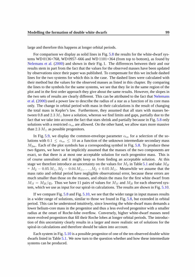
In Fig.5.9, we display the common-envelope parameterαce for a selection of the so-lutions with0.1 ≤ αce ≤ 10 as a function of the unknown intermediate secondary massM2m. Each of the plot symbols has a corresponding symbol in Fig.5.8. To produce thesetwo figures, we have so far implicitly assumed that the massesof the two components areexact, so that there is at most one acceptable solution for each progenitor mass. This isof course unrealistic and it might keep us from finding an acceptable solution. At thisstage we therefore introduce an uncertainty on the values for M2 in Table5.1and takeM2f
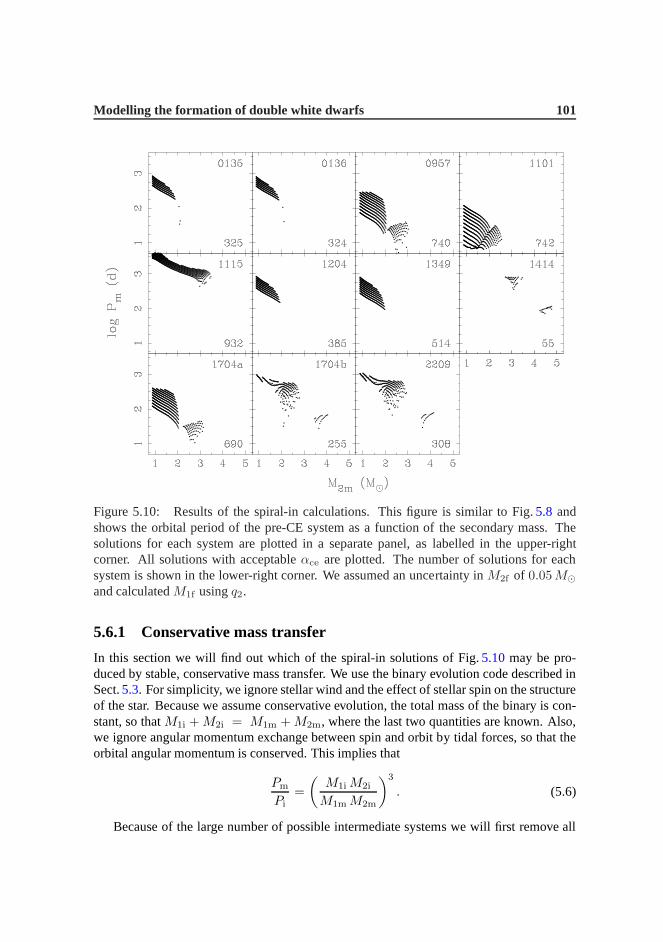
= M2 − 0.05 M⊙, M2 − 0.04 M⊙, . . . , M2 + 0.05 M⊙. Meanwhile we assume that themass ratio and orbital period have negligible observational error, because these errors aremuch smaller than those on the masses, and obtain the mass forthe first white dwarf fromM1f = M2f/q2. Thus we have 11 pairs of values forM1f andM2f for each observed sys-tem, which we use as input for our spiral-in calculations. The results are shown in Fig.5.10.
If we compare Fig.5.8and Fig.5.10, we see that the wider range in input masses resultsin a wider range of solutions, similar to those we found in Fig.5.8, but extended in orbitalperiod. This can be understood intuitively, since loweringthe white-dwarf mass demands alower helium-core mass in the progenitor and thus a less evolved progenitor with a smallerradius at the onset of Roche-lobe overflow. Conversely, higher white-dwarf masses needmore evolved progenitors that fill their Roche lobes at longer orbital periods. The introduc-tion of this uncertainty clearly results in a larger and morerealistic set of solutions for thespiral-in calculations and therefore should be taken into account.
Each system in Fig.5.10is a possible progenitor of one of the ten observed double whitedwarfs listed in Table5.1. We now turn to the question whether and how these intermediatesystems can be produced.

100 Chapter 5
Figure 5.9: The logarithm of the common-envelope parameterαce for the solutions ofthe spiral-in calculations shown in Fig.5.8. Different symbols represent different observedsystems. ForM2m < 2.5 M⊙ every third solution is plotted only.
5.6 First mass-transfer phase
The solutions of the spiral-in calculations we found in the previous section are in our nomen-clatureintermediate binaries, that consist of one white dwarf and a non-degenerate com-panion. In this section we will look for an initial binary that consists of two zero-age main-sequence (ZAMS) stars of which the primary evolves, fills itsRoche lobe, loses its hydrogenenvelope, possibly transfers it to the secondary, so that one of the intermediate binaries ofFig.5.10 is produced. The nature of this first mass transfer is a prioriunknown. In thefollowing subsections we will consider (1) stable and conservative mass transfer that willresult in expansion of the orbit in most cases, (2) a common envelope with spiral-in basedon energy balance (see Eq.5.4) that usually gives rise to appreciable orbital shrinkage and(3) envelope ejection due to dynamically unstable mass lossbased on angular-momentumbalance, as introduced byPaczynski & Ziołkowski(1967) and already used byNelemanset al.(2000) for the same purpose, which can take place without much change in the orbitalperiod.
Modelling the formation of double white dwarfs 101
Figure 5.10: Results of the spiral-in calculations. This figure is similar to Fig.5.8 andshows the orbital period of the pre-CE system as a function ofthe secondary mass. Thesolutions for each system are plotted in a separate panel, aslabelled in the upper-rightcorner. All solutions with acceptableαce are plotted. The number of solutions for eachsystem is shown in the lower-right corner. We assumed an uncertainty in M2f of 0.05 M⊙
and calculatedM1f usingq2.
5.6.1 Conservative mass transfer
In this section we will find out which of the spiral-in solutions of Fig.5.10may be pro-duced by stable, conservative mass transfer. We use the binary evolution code described inSect.5.3. For simplicity, we ignore stellar wind and the effect of stellar spin on the structureof the star. Because we assume conservative evolution, the total mass of the binary is con-stant, so thatM1i + M2i = M1m + M2m, where the last two quantities are known. Also,we ignore angular momentum exchange between spin and orbit by tidal forces, so that theorbital angular momentum is conserved. This implies that
Pm
Pi
=
(
M1i M2i
M1m M2m
)3
. (5.6)
Because of the large number of possible intermediate systems we will first remove all
102 Chapter 5
such systems for which it can a priori be shown that they cannot be produced by conservativemass transfer. These systems have orbital periods that are either too short or too long to beformed this way. We can find a lower limit to the intermediate period as a function ofsecondary massM2m using the fact that the total mass of the initial system must be equalto the sum of the mass of the observed white dwarfM1 andM2m. We distributed this massequally over two ZAMS stars and set the Roche-lobe radii equal to the two ZAMS radii. Bysubstituting the initial and desired masses in Eq.5.6 we find a lower limit to the period ofthe intermediate binary, which we will callPmin.
An upper limit to the intermediate periodPm can also be obtained. In order to do this,we note that the maximum orbital period after conservative mass transfer for a given binarymass is obtained for an optimum initial mass ratioq2i,opt = 0.62 (Nelemans et al. 2000).We can therefore calculate the massesM1i,opt andM2i,opt of the initial binary that evolvesto that maximum intermediate period by distributing the total system mass (M1 + M2m)according to the mass ratioq2i,opt. The optimum initial period is the maximum period atwhich stable mass transfer can still occur in a binary with massesM1i,opt andM2i,opt. Thisis the orbital period at which the donor star fills its Roche lobe just before it reaches thebase of the giant branch (BGB). We use the conditions byHurley et al.(2000) who definethis point as the moment where the mass of the convective envelopeMCE exceeds a certainfraction of the total mass of the hydrogen envelopeME for the first time:
MCE = 25
ME, M1i,opt ≤ 1.995 M⊙,MCE = 1
3ME, M1i,opt > 1.995 M⊙,
(5.7)
for Z = 0.02. We then find from our grid of Sect.5.4the two single-star models with massesthat bracketM1i,opt and interpolate within these models to find the radii of thesestars wherethe condition of Eq.5.7 is fulfilled for the first time. Subsequently, we interpolateagainbetween these two bracketing models to find the radius of the star with the desired mass atthe base of the giant branch (RBGB). By assuming that this radius is equal to the Roche-loberadius and using Eq.5.5, the initial masses and period that lead to the maximum intermediateperiod are known and we can use Eq.5.6to find this upper limit to the intermediate period,which we will call Pmax, as a function of the secondary mass. All intermediate systemsthat result from our spiral-in calculations and have longerorbital periods thanPmax cannotresult from conservative mass transfer.
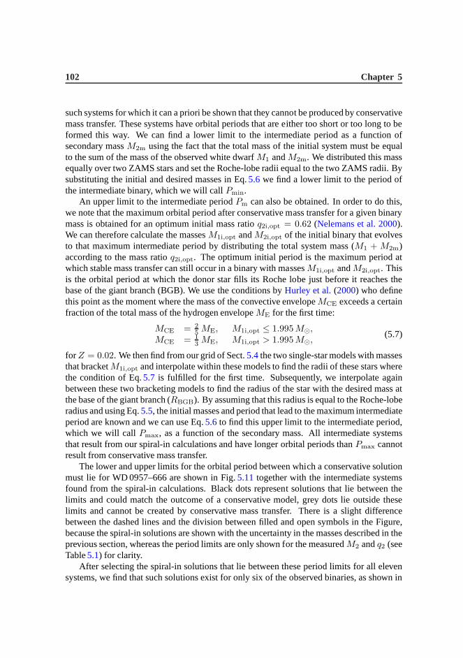
The lower and upper limits for the orbital period between which a conservative solutionmust lie for WD 0957–666 are shown in Fig.5.11together with the intermediate systemsfound from the spiral-in calculations. Black dots represent solutions that lie between thelimits and could match the outcome of a conservative model, grey dots lie outside theselimits and cannot be created by conservative mass transfer.There is a slight differencebetween the dashed lines and the division between filled and open symbols in the Figure,because the spiral-in solutions are shown with the uncertainty in the masses described in theprevious section, whereas the period limits are only shown for the measuredM2 andq2 (seeTable5.1) for clarity.
After selecting the spiral-in solutions that lie between these period limits for all elevensystems, we find that such solutions exist for only six of the observed binaries, as shown in

Modelling the formation of double white dwarfs 103
Figure 5.11: Results of the spiral-in calculations for WD 0957–666 with period limits fora conservative first mass transfer. This figure contains the same data as the third panel inFig.5.10(symbols) plus the period limitsPmin andPmax (dashed lines). The solutions thatlie between these limits are shown in black, the others in grey. See the main text for details.
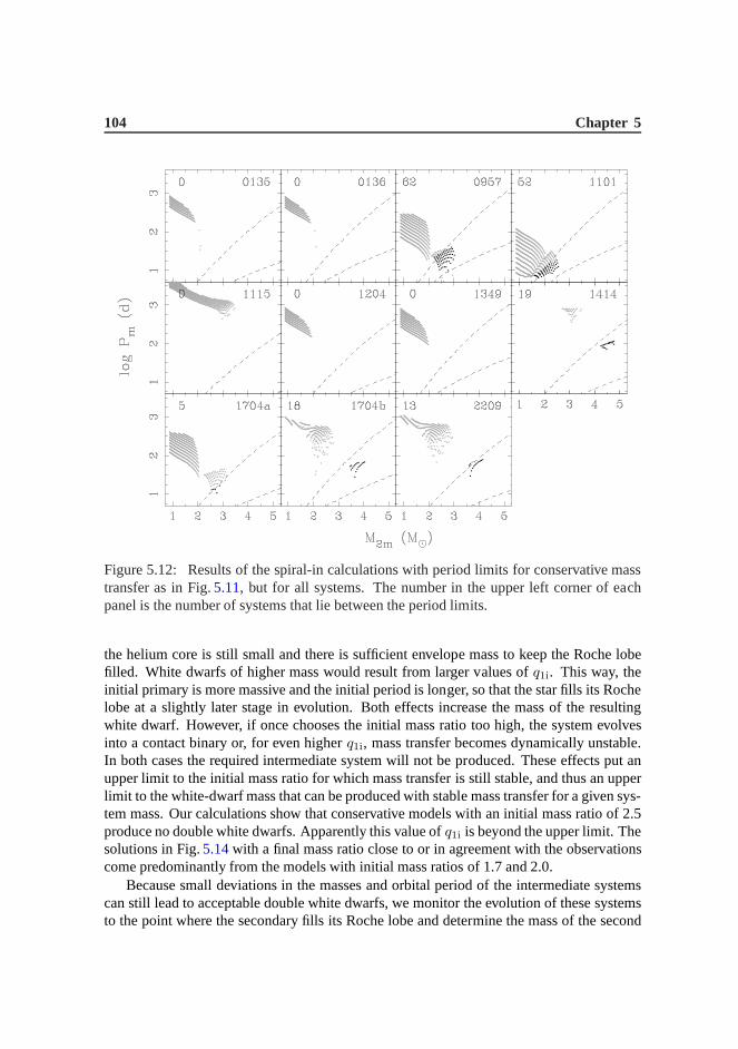
Fig.5.12. We tried to model these intermediate systems with the binary evolution codedescribed in Sect.5.3. Because of the large number of allowed spiral-in solutionsforWD 0957–666 and WD 1101+364, we decided to model about half ofthe solutions forthese two systems and all of the solutions for the other four.Because we assume that duringthis part of the evolution mass and orbital angular momentumare conserved, the only freeparameter is the initial mass ratioq1i ≡ M1i/M2i. For each of the spiral-in solutions weselected, we chose five different values forq1i, evenly spread in the logarithm: 1.1, 1.3, 1.7,2.0 and 2.5. The total number of conservative models that we calculated is 570, of which270 resulted in a double white dwarf. The majority of the resteither experienced dynamicalmass transfer or evolved into a contact system. A few models were discarded because ofnumerical problems. The results of the calculations for theconservative first mass transferare compared to the solutions of the spiral-in calculationsin Fig.5.13.
The systems that result from our conservative models generally have longer orbital pe-riods than the intermediate systems that we are looking for.This means that stable masstransfer in the models continues beyond the point where the desired masses and orbital pe-riod are reached. The result is thatM1m is too small and thatM2m andPm are too large.The reason that mass transfer continues is that the donor star is not yet sufficiently evolved:
104 Chapter 5
Figure 5.12: Results of the spiral-in calculations with period limits for conservative masstransfer as in Fig.5.11, but for all systems. The number in the upper left corner of eachpanel is the number of systems that lie between the period limits.
the helium core is still small and there is sufficient envelope mass to keep the Roche lobefilled. White dwarfs of higher mass would result from larger values ofq1i. This way, theinitial primary is more massive and the initial period is longer, so that the star fills its Rochelobe at a slightly later stage in evolution. Both effects increase the mass of the resultingwhite dwarf. However, if once chooses the initial mass ratiotoo high, the system evolvesinto a contact binary or, for even higherq1i, mass transfer becomes dynamically unstable.In both cases the required intermediate system will not be produced. These effects put anupper limit to the initial mass ratio for which mass transferis still stable, and thus an upperlimit to the white-dwarf mass that can be produced with stable mass transfer for a given sys-tem mass. Our calculations show that conservative models with an initial mass ratio of 2.5produce no double white dwarfs. Apparently this value ofq1i is beyond the upper limit. Thesolutions in Fig.5.14with a final mass ratio close to or in agreement with the observationscome predominantly from the models with initial mass ratiosof 1.7 and 2.0.
Because small deviations in the masses and orbital period ofthe intermediate systemscan still lead to acceptable double white dwarfs, we monitorthe evolution of these systemsto the point where the secondary fills its Roche lobe and determine the mass of the second

Modelling the formation of double white dwarfs 105
Figure 5.13: Results of the spiral-in calculations (grey symbols), obtained as in Fig.5.11,and the solutions of calculations of conservative evolution (black symbols). Only the sixsystems shown have spiral-in solutions within the period limits (see Fig.5.12). The numbersin the lower left and lower right corners are the numbers of plotted spiral-in solutions andconservative solutions respectively.
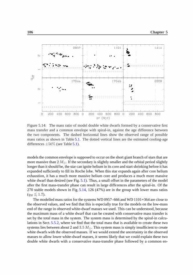
white dwarfM2f from the helium-core mass of the secondary at that point. Because thesecondary in the intermediate binary is slightly too massive in most cases, it is smaller at agiven core mass (see Fig.5.1) so that the mass of the second white dwarf becomes larger thandesired. Combined with an undermassive first white dwarf this results in a too large massratio q2f . This is shown in Fig.5.14, where the values forq2f for our conservative modelsare compared to the observations. The Figure also shows the difference in age of the systembetween the moment where the second white dwarf was formed and the moment whenthe first white dwarf was formed (∆τ ). This difference should be similar to the observeddifference in cooling age between the two components of the binary (see Table5.1). Thevertical dotted lines show this observed cooling-age difference with an uncertainty of 50%.
Figure5.14shows that of the six systems presented, only two have a mass ratio withinthe observed range, although values for the other systems may be close. We see that the massratios of the solutions for most of the systems are divided intwo groups and the differencein mass ratio can amount to a factor of 2 between them. The division arises because in most
106 Chapter 5
Figure 5.14: The mass ratio of model double white dwarfs formed by a conservative firstmass transfer and a common envelope with spiral-in, againstthe age difference betweenthe two components. The dashed horizontal lines show the observed range of possiblemass ratios as shown in Table5.1. The dotted vertical lines are the estimated cooling-agedifferences±50% (see Table5.1).
models the common envelope is supposed to occur on the short giant branch of stars that aremore massive than2 M⊙. If the secondary is slightly smaller and the orbital periodslightlylonger than it should be, the star can ignite helium in its core and start shrinking before it hasexpanded sufficiently to fill its Roche lobe. When this star expands again after core heliumexhaustion, it has a much more massive helium core and produces a much more massivewhite dwarf than desired (see Fig.5.1). Thus, a small offset in the parameters of the modelafter the first mass-transfer phase can result in large differences after the spiral-in. Of the270 stable models shown in Fig.5.14, 126 (47%) are in the group with lower mass ratios(q2f ∼< 1.7).
The modelled mass ratios for the systems WD 0957–666 and WD 1101+364 are close tothe observed values, and we find that this is especially true for the models on the low-massend of the range in observed white-dwarf masses we used. Thiscan be understood, becausethe maximum mass of a white dwarf that can be created with conservative mass transfer isset by the total mass in the system. The system mass is determined by the spiral-in calcu-lations in Sect.5.5.2, where we find that the total mass that is available to create these twosystems lies between about2 and3.5 M⊙. This system mass is simply insufficient to createwhite dwarfs with the observed masses. If we would extend theuncertainty in the observedmasses to allow lower white-dwarf masses, it seems likely that we could explain these twodouble white dwarfs with a conservative mass-transfer phase followed by a common en-

Modelling the formation of double white dwarfs 107
velope with spiral-in. The same could possibly be achieved with stable, non-conservativemass transfer. Losing mass from the system stabilises the mass transfer, so that it can stillbe stable for slightly longer initial periods, and allows higher initial primary masses. Botheffects result in higher white-dwarf masses.
All 126 stable solutions in the lower group of mass ratios (q2f ∼< 1.7) haveαce > 1and 83 (66%) haveαce < 5. If we become more demanding and insist thatαce should beless than 2, we are left with 14 solutions, all for WD 0957–666. These solutions all haveαce > 1.6. If we additionally demand that the age difference of these models be less than50% from the observed cooling-age difference, only 6 solutions are left with age differencesroughly between 190 and 410 Myr,αce > 1.8 and1.32 ≤ q2f ≤ 1.44.
We conclude that although the evolutionary channel of conservative mass transfer fol-lowed by a spiral-in can explain some of the observed systems, evolution along this channelcannot produce all observed double white dwarfs. We must therefore reject this formationchannel as the single mechanism to create the white-dwarf binaries. The reason that thismechanism fails to explain some of the observed white dwarfsis that the observed massesfor the first white dwarfs in these systems are too high to be explained by conservative masstransfer in a binary with the total mass that is set by the spiral-in calculations. Allowing formass loss from the system during mass transfer could result in better matches for this mech-anism. However it is clear from Fig.5.12that this will certainly not work for at least 5 of the10 observed systems because their orbital periods are too large. We will need to considerother mechanisms in addition to stable mass transfer to produce the observed white-dwarfprimaries for these systems.
5.6.2 Unstable mass transfer
In this section we try to explain the formation of the first white dwarf in the intermediatesystems shown in Fig.5.10by unstable mass transfer. Mass transfer occurs on the dynam-ical timescale if the donor is evolved and has a deep convective envelope. There are twoprescriptions that predict the change in orbital period in such an event. The first is a clas-sical common envelope with a spiral-in, based on energy conservation as we have used inSect.5.5. The second prescription was introduced byNelemans et al.(2000) and furtherexplored byNelemans & Tout(2005) and uses angular-momentum balance to calculate thechange in orbital period. Where the first prescription results in a strong orbital shrinkage(spiral-in) for all systems, in the second mechanism this isnot necessarily the case so thatthe orbital period may hardly change while the envelope of the donor star is lost.
In both scenarios we are looking for an initial binary of which the components havemassesM1i and M2i. The primary will evolve fastest, fill its Roche lobe and eject itsenvelope due to dynamically unstable mass loss, so that its core becomes exposed and formsa white dwarf with massM1m. We assume that the mass of the secondary star does notchange during this process, so thatM2i = M2m. We use the model stars from Sect.5.4.1as the possible progenitors for the first white dwarf. The orbital period before the envelopeejection is again determined by setting the radius of the model star equal to the Roche-lobe
108 Chapter 5
radius and applying Eq.5.5, where the subscripts ‘m’ must be replaced by ‘i’.Because we demand thatM1i > M2i, the original secondary can be any but the most
massive star from our grid and the total number of possible binaries in our grid is∑198
n=1 n =19701 for each system we want to model. The total number of systems that we try to modelis 121: the 11 observed systems (the 10 from Table5.1 plus the system WD 1704+481b)times 11 different assumptions for the masses of the observed stars (between±0.05 M⊙
from the observed value). We have thus tried slightly less than 2.4 million initial binariesto find acceptable progenitors to these systems. All these possible progenitor systems havebeen filtered by the following criteria, in addition to the ones already mentioned in Sect.5.5:
1. the radius of the star is larger than the radius at the base of the giant branchR >RBGB, which point is defined by Eq.5.7,
2. the mass ratio is larger than the critical mass ratio for dynamical mass transferq >qcrit as defined by Eq. 57 ofHurley et al.(2002). Together with the previous criterium,this ensures that the mass transfer can be considered to proceed on the dynamicaltimescale,
3. the time since the ZAMS after which the first white dwarf is createdτ1 is less thanthe same for the second white dwarf (τ2) and, additionally,τ2 < 13 Gyr.
After we filter the approximately 2.4 million possible progenitor systems with the crite-ria above, about 204,000 systems are left in the sample (8.5%) for which two subsequentenvelope-ejection scenarios could result in the desired masses, provided that we can some-how explain the change in orbital period that is needed to obtain the observed periods. Foreach of the two prescriptions for dynamical mass loss we willsee whether this sample con-tains physically acceptable solutions in the sections thatfollow.
Classical common envelope with spiral-in
The treatment of a classical common envelope with spiral-inbased on energy conservationhas been described in detail in Sect.5.5 and therefore need not be reiterated here. In thecalculations described above, Eq.5.4provides us with the parameterαce1 for the first spiral-in. In order to use Eq.5.4the subscripts ‘m’ must be replaced by ‘i’ and the subscripts‘f’ by‘m’. The values of the common-envelope parameter for the first spiral-in must be physicallyacceptable and we demand that0.1≤αce1≤10. When we apply this criterion to the resultsof our calculations, only 25 possible progenitors out of the204,000 binaries in our samplesurvive. All 25 survivors are solutions for WD 0135–052 and haveαce1 ∼> 2.5.
We find that of the systems that pass the criterion in the second spiral-in and have0.1≤αce2≤10, most (99%) need a negativeαce1 in order to satisfy Eq.5.4, so that we reject them.We can clearly conclude that the scenario of two subsequent classical common envelopeswith spiral-in can be rejected as the formation mechanism for any of the observed doublewhite dwarfs. This confirms the conclusions ofNelemans et al.(2000) andNelemans &Tout(2005), based on the value of the productαce λenv, whereλenv is the envelope-structureparameter defined in Eq.5.2.
Modelling the formation of double white dwarfs 109
Envelope ejection with angular-momentum balance
The idea to determine the change in orbital period in a commonenvelope from balance ofangular momentum originates fromPaczynski & Ziołkowski(1967). In Nelemans et al.(2000) andNelemans & Tout(2005) the mechanism was used to model observed doublewhite dwarfs. The principle is similar to that of a classicalcommon envelope, here withan efficiency parameter that we will callγ in the general case. In this section we will usethree slightly different prescriptions for mass loss with angular-momentum balance requir-ing three different definitions ofγ. For all three mechanisms the mass loss of the donor isdynamically unstable and its envelope is ejected from the system. Because not all of thesemechanisms necessarily involve an envelope that engulfs both stars, we shall refer to themas envelope ejection or dynamical mass loss rather than common-envelope evolution. Thefirst mechanism is that defined byNelemans et al.(2000), where a common envelope isestablished first, after which the mass is lost from its surface. The mass thus carries theaverage angular momentum of the system and we will call the parameter for this mecha-nismγs. In the second mechanism the mass is first transferred and then re-emitted with thespecific angular momentum of the accretor. We will designateγa for this mechanism. Inthe third mechanism the mass is lost directly from the donor in an isotropic wind and thecorresponding parameter isγd. We will call the companion to the donor star ‘accretor’, evenif no matter is actually accreted.
The prescription for dynamical mass loss with the specific angular momentum of thesystem as the mechanism for the first mass-transfer phase, using this and earlier subscriptconventions, is:
Ji − Jm
Ji
= γs1
M1i − M1m
M1i + M2i
, (5.8)
whereJ is the total orbital angular momentum (Nelemans et al. 2000). Our demands for aphysically acceptable solution to explain the observed binaries is now0.1≤γs1≤10 for thefirst envelope ejection and0.1≤ αce2 ≤ 10 for the second. From the set of about 204,000solutions we found above, almost 150,000 (72%) meet these demands and nearly 134,000solutions (66%) have values forγs1 between 0.5 and 2, in which all observed systems arerepresented.
We tried to constrain the ranges forγs1 andαce2 as much as possible, thereby keeping atleast one solution for each observed system. We can write these ranges as(γ0−
∆γ2
, γ0+∆γ2
)
and(α0 −∆α2
, α0 + ∆α2
), whereγ0 andα0 are the central values and∆γ and∆α are thewidths of each range. We independently variedγ0 andα0 and for each pair we took thesmallest values of∆γ and∆α for which there is at least one solution for each observedsystem that lies within both ranges. The set of smallest ranges thus obtained is consideredto be the best range forγs1 andαce2 that can explain all systems. Because it is harder totrifle with the angular-momentum budget than with that of energy, we kept the relative widthof the range forγs1 twice as small as that forαce2 (2∆γ
γ0= ∆α
α0). Our calculations show that
changing this factor merely redistributes the widths over the two ranges without affectingthe central values much and thus precisely which factor we use seems to be unimportant forthe result. We find that the set of narrowest ranges that contain a solution for each system is
110 Chapter 5
1.45≤γs1≤1.58 and0.61≤αce2≤0.72. These results are plotted in Fig.5.15.We can alternatively treat the second envelope ejection with the angular-momentum
prescription as well, where we need to introduce a factorγs2 by replacing all subscripts ‘m’by ‘f’ and all subscripts ‘i’ by ‘m’ in Eq.5.8. Again we search for the narrowest rangesof γs1 andγs2 that contain at least one solution per observed system. We now force therelative widths of the two ranges to be equal. The best solution is then1.16≤ γs1 ≤ 1.22and1.62≤γs2≤1.69.
In both prescriptions above (γs1αce2 andγs1γs2) we find that the values forγ lie signif-icantly above unity. This is in accordance with the findings of Nelemans et al.(2000) andNelemans & Tout(2005), but slightly discomforting because there is no obvious physicalmechanism that can transfer this extra angular momentum to the gas of the envelope. Wewill therefore rewrite Eq.5.8 for the case where the mass is lost with the specific angularmomentum of one of the stars in the binary, so that we can expect thatγ ≈ 1. In order to dothis we use the equations derived bySoberman et al.(1997) in their Section 2.1. We ignorethe finite sizes of the star by puttingAw = 1 and assume that no matter is accreted, so thatαw + βw = 1 andǫw = 0, where we introduced the subscript ‘w’ to avoid confusion withαce. Their Eq. 24 then gives (replacing their notation by ours):
Jm
Ji
=
(
qm
qi
)αw 1 + qi
1 + qm
, (5.9)
where we will consider the cases whereαw = 0 (henceβw = 1), describing isotropic re-emission by the accretor, andαw = 1 for an isotropic wind from the donor. Theirq isdefined asmdonor/maccretor. We can now rewrite Eq.5.8for these two cases:
Ji − Jm
Ji
= γa1
M1i − M1m
M1m + M2m
(αw = 0), (5.10)
Ji − Jm
Ji
= γd1
M1i − M1m
M1m + M2m
M2i
M1i
(αw = 1). (5.11)
By comparing Eq.5.8 to Eq.5.10, we can directly see that for an envelope ejection withgiven masses and angular momenta,γa < γs must hold in order to keep it satisfying theequation. For Eq.5.11, this is not necessarily true for a first envelope ejection but the effectis even stronger for all second envelope ejections considered in this chapter. The results ofthe analysis described above, but now for the modified definitions ofγ, for theγα andγγscenarios, each withαw = 0 (isotropic re-emission) andαw = 1 (donor wind) are shownin Table5.2and compared to the previous results.
We see that the values forγ change drastically, as may be expected. The fact that thevalues forαce change slightly has to do with the fact that we now select different solutionsto the calculations than before. Numerically, the fifth solution in the table seems the mostattractive:γd1 ≈ 1.0 andαce2 ≈ 0.6. Although the value forαce2 is lower than unity, itmay not be unrealistic that 40 % of the freed orbital energy isemitted by radiation. This isthe scenario where the mass is lost in an isotropic wind by thedonor in the first dynamical

Modelling the formation of double white dwarfs 111
Figure 5.15: Solutions for the double dynamical mass-loss scenario for each system. Eachdot represents one system that evolves through an episode ofdynamical mass loss withγs1 and then a common envelope with spiral-in withαce2 to form one of the observedwhite dwarfs.Upper panel:(a): the value forlog γs1 for the first envelope ejection for allsolutions with0.1 ≤ γs1 ≤ 10 and0.1 ≤ αce2 ≤ 10. Solutions with0.61 ≤ αce2 ≤ 0.72(the dashed lines in (b)) are plotted as large dots, the rest as small ones.Lower panel:(b):the value forlog αce2 for the second envelope ejection for the same set of solutions. Here,the large dots have1.45 ≤ γs1 ≤ 1.58 (the dashed lines in (a)). The smallest set with atleast one solution for each system is the intersection of these two sets (the large dots thatlie between the dashed lines). The vertical position of eachdot within its line shows thedeviation from the observed secondary massM2: M2f = M2−0.05 M⊙ for the lower dots,M2f = M2 + 0.05 M⊙ for the upper. The Figure is made afterNelemans & Tout(2005).

112 Chapter 5
Prescription γ1 γ0,1 γ2/αce2 γ0,2/α0,2
γs1αce2 1.45–1.58 1.52 α : 0.61–0.72 α : 0.66γs1γs2 1.16–1.22 1.19 γ : 1.62–1.69 γ : 1.65γa1αce2 0.81–0.94 0.88 α : 0.50–0.68 α : 0.59γa1γa2 0.50–0.52 0.51 γ : 0.68–0.70 γ : 0.69γd1αce2 0.92–1.08 1.00 α : 0.47–0.64 α : 0.56γd1γd2 0.91–1.07 0.99 γ : 2.55–3.02 γ : 2.78
Table 5.2: Narrowest ranges forγ andαce that contain at least one solution to the envelope-ejection scenario per observed system and their central values. The six different prescrip-tions are explained in the main text.
mass-loss episode and the second mass loss is a canonical common envelope with spiral-in.We also see that the best solutions with a second envelope ejection based on the angular-momentum prescription obtained with this method has valuesfor γ that lie much fartherfrom unity than theγ-values for theγα-scenarios.
5.6.3 Formation by multiple mechanisms
So far, we assumed that all ten observed double white dwarfs were formed by one and thesame mechanism. Although some mechanisms are clearly better in explaining the formationof all the observed systems than others, none of them is completely satisfactory, mainlybecause the parametersγ or αce are far from the desired values. Furthermore, there is noreason why the ten systems should all have been formed by the same mechanism in natureif there are several options available. We therefore slightly change our strategy here byassuming that different envelope-ejection prescriptions, described in Sect.5.6.2, can play arole in the formation of the observed systems.
For the dynamical mass loss, we now demand thatγ andαce are close to unity. Becauseangular momentum should be better conserved than energy, weaccept solutions with0.95<γ < 1.05 and0.90 < αce < 1.10, except for the mechanism described by Eq.5.8, for whichNelemans & Tout(2005) show that all systems can be explained with1.50 < γ < 1.75,which we reduce to1.54 < γ < 1.71 to give it the same relative width. For each observedsystem and each mechanism, we look whether there is at least one solution with a envelope-ejection parameter within these ranges. The results are shown as the first symbol in eachentry of Table5.3. The plus signs show which mechanism can explain the mass ratio ofan observed double white dwarf. The table shows that although none of the mechanismscan explain all observed systems within the chosen ranges ofγ andαce, the second-lastcolumn shows that a combination of these mechanisms can. Thetable also indicates thatmechanisms containing onlyγs and none of the otherγ’s cannot explain all systems. Thesame is true forγa andγd. If we expand the chosen ranges forγ andαce with a factor oftwo, our calculations show that the mechanismsγsγs andγdγa can explain the mass ratiosof all systems. Expanding the allowed ranges in this way morethan quadruples the total

Modelling the formation of double white dwarfs 113
System 1: 2: 3: 4: 5: 6: Opt. Bestγsαce γsγs γaαce γaγa γdαce γdγa res. mech.
0135 −/− +/∼ −/− −/− +/∼ +/− +/∼ 2,50136 +/+ +/+ +/∼ −/− +/+ −/− +/+ 1,2,50957 +/+ +/+ +/+ +/+ +/+ +/∼ +/+ 1–51101 +/∼ +/− +/∼ +/− −/− −/− +/∼ 1,31115 +/∼ +/∼ +/+ +/∼ +/+ −/− +/+ 3,5
1204 −/− −/− −/− −/− +/− +/− +/− 5,61349 +/+ +/+ +/+ −/− +/+ −/− +/+ 1,2,3,51414 −/− −/− −/− −/− −/− +/+ +/+ 61704a +/− +/− −/− +/− −/− +/− +/− 1,2,4,61704b +/− +/− +/− +/− +/− +/− +/− 1–62209 −/− +/+ −/− +/+ −/− +/∼ +/+ 2,4
Table 5.3: Comparison of the different mechanisms used to reconstruct the observed doublewhite dwarfs. The symbols+,∼ and− mean that the model solutions are in good, moderateor bad agreement with the observations. The first of the two symbols in each column isbased on the mass ratio only and the second includes the age difference. The method forobtaining the first symbol in each entry is described in Sect.5.6.3, that for the second symbolin Sect.5.6.4. The symbols in the headers of the columns labelled 1–6 are explained in themain text. The columns forγaγd andγdγd were left out because they do not contain anysolutions. The last two columns show the optimum result and the mechanisms that give thisresult (1–6).
number of solutions from 7866 to 36 867.
5.6.4 Constraining the age difference
The large number of solutions found in the previous section allows us to increase the numberof selection criteria that we use to qualify a solution as physically acceptable. We nowinclude the age difference of the components in our model systems and demand that it iscomparable to the observed cooling-age difference for thatsystem. The age difference inour models is the difference in age at which each of the components fills its Roche lobe andcauses dynamical mass loss.
Table5.4lists the number of model solutions for each mechanism and each system. Thecolumns labelled 1–6 are the same as those in Table5.3. The first number in each of thesecolumns is the number of solutions that is found within the same ranges forγ andαce aswe used in Table5.3. This means that a minus sign in that table corresponds to a zero inTable5.4. Behind the entries with a positive number of solutions the range of age differencethat these solutions span is shown. Again, the columns forγaγd andγdγd are not displayed,because they do not contain any solutions for any system. We have to expand theγ-ranges
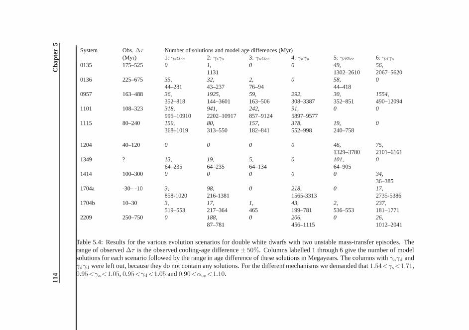
114
Cha
pter
5System Obs.∆τ Number of solutions and model age differences (Myr)
(Myr) 1: γsαce 2: γsγs 3: γaαce 4: γaγa 5: γdαce 6: γdγa
0135 175–525 0 1, 0 0 49, 56,1131 1302–2610 2067–5620
0136 225–675 35, 32, 2, 0 58, 044–281 43–237 76–94 44–418
0957 163–488 36, 1925, 59, 292, 30, 1554,352–818 144–3601 163–506 308–3387 352–851 490–12094
1101 108–323 318, 941, 242, 91, 0 0995–10910 2202–10917 857–9124 5897–9577
1115 80–240 159, 80, 157, 378, 19, 0368–1019 313–550 182–841 552–998 240–758
1204 40–120 0 0 0 0 46, 75,1329–3780 2101–6161
1349 ? 13, 19, 5, 0 101, 064–235 64–235 64–134 64–905
1414 100–300 0 0 0 0 0 34,36–385
1704a -30– -10 3, 98, 0 218, 0 17,858-1020 216-1381 1565-3313 2735-5386
1704b 10–30 3, 17, 1, 43, 2, 237,519–553 217–364 465 199–781 536–553 181–1771
2209 250–750 0 188, 0 206, 0 26,87–781 456–1115 1012–2041
Table 5.4: Results for the various evolution scenarios for double white dwarfs with two unstable mass-transfer episodes. Therange of observed∆τ is the observed cooling-age difference± 50%. Columns labelled 1 through 6 give the number of modelsolutions for each scenario followed by the range in age difference of these solutions in Megayears. The columns withγaγd andγdγd were left out, because they do not contain any solutions. Forthe different mechanisms we demanded that1.54<γs<1.71,0.95<γa<1.05, 0.95<γd<1.05 and0.90<αce<1.10.
Modelling the formation of double white dwarfs 115
to 0.25–1.75 in order to get the first solution for just a single system with one of these twomechanisms. All mechanisms that are listed in Table5.4 provide a solution for more thanone observed system, and each observed system has at least one mechanism that providesit with a solution. The number of solutions per combination of mechanism and observedsystem ranges from zero to several hundreds and the age differences of the accepted modelslie between 36 Myr and more than 12 Gyr.
We will use Table5.4to compare the age differences of the models to the observed val-ues and use this comparison to judge the ‘quality’ of the model solutions. We will assumethat if the age difference in the model lies within 50% of the measured cooling-age differ-ence (the range in the second column of Table5.4) that this is a good agreement which wewill assign the symbol ‘+’. If the difference is larger than that, but smaller than a factor offive we will call it ‘close’ and assign a ‘∼’. Cases where the nearest solution has an agedifference that is more than a factor of five from the observedvalue is considered ‘bad’ andassigned the symbol ‘−’. If we do this for all cases, we obtain the second symbol for eachentry in Table5.3, which we can use to directly compare the quality of the solutions for eachmechanism and each observed system.
We find that these results are robust, in the sense that if we expand the ranges forγandαce with a factor of two, the optimum result does not change, although there are moremechanisms contributing to this result,i.e. the column ‘opt. result’ remains unchanged,while the number of labels in the last column increases. The same is even true if we expandthe ranges forαce with a factor of ten instead of two. If we use a factor of 2 in stead of 5for the upper limit of a ‘close solution’, we need to expand the ranges forγ andαce witha factor of 2.6 to get tildes at the same places in the column ‘optimum result’ as shown inTable5.3.
We conclude that our models can form double white dwarfs withthe observed massesand orbital periods if we invoke multiple formation mechanisms. Our calculations showthat if we double the allowed ranges forγ andαce with respect to those used in Tables5.3and5.4, it is even possible to form all observed systems with mechanismsγsγs only orγdγa
only. If we demand in addition that the age differences of themodel systems lie within 50%of the observed value, we can still explain the formation of most observed systems, whilefor some double white dwarfs this becomes difficult. This is the case with WD 0135–052,WD 1204+450, WD 1704+481b and to a lesser extent WD 1101+364.These four systemscan usually either be explained with an acceptable age difference but a value forγ that isoff, or an acceptableγ and an age difference that lies (sometimes much) more that 50%from the observed value.
5.6.5 Description of the individual solutions
The goal of this research is, of course, to find out whether we can somehow explain theformation of the observed double white dwarfs. If this is thecase, we hope to learn firstlywhich mechanisms govern this formation and secondly what the progenitor systems are thatevolve to the observed white-dwarf binaries. Although we donot find one mechanism that
116 Chapter 5
can explain all observed systems in a satisfying way, we present here the evolution of someof the best solutions among our calculations. We list the fivemain parameters that describethe evolutionary scenario of a solution (two initial masses, the initial period and the twoenvelope-ejection parameters) and two minor ones (the actual final masses that the modelsgive) in a table. Because we present solutions for six different formation mechanisms andeleven observed systems that may have more than one ‘best’ solution this table is quite large.This is particularly the case because we want to remove the arbitrarily chosen boundariesthat we have used so far to qualify a solution. We therefore list at least one solution permechanism per system, independent of how far its parameterslie from the preferred values.We chose to present the complete table as Table5.6 in Sect.5.9and give an excerpt of it inTable5.5. In this way, the reader may verify how particular models do or do not work.
We manually picked the ‘best’ solutions for a given combination of formation mecha-nism and observed system, in the sense that the solution has aγ close to unity (or, in caseof γs, close to 1.63), anαce close to the range of 0.5–1.0 and an age difference that is closeto the observed value. In the cases where there are differentsolutions that each excel in adifferent one of these three properties, we may present morethan one solution. If there areseveral solutions that are similar on these grounds, we prefer those with lower initial masses.We then leave it to the reader to judge whether these solutions are acceptable. The valuesfor q2f andPf are identical to the value listed in Table5.1 and therefore not shown in Ta-ble5.5. The intermediate masses are also left out of the table, because no matter is accretedduring the dynamical mass loss and thusM1m = M1f andM2m = M2i in our models. Thenumbering of the solutions in the excerpted table is the sameas in the complete version.
We tabulate 120 solutions in total. The initial binaries have primary masses between1.09M⊙ and 5.42M⊙, though there are only two solutions withM1i > 4 M⊙. Of the 120solutions, 50% have an initial primary mass less than 2M⊙ and 87% of the primaries areless massive than 3M⊙. Thus, the models suggest that the double white dwarfs are formedby low-mass stars, as may be required to explain the observednumbers of these binaries.Of the initial systems, 90% have orbital periods between 10 and 1000 days. All proposedsolutions undergo a first envelope ejection described by angular-momentumbalance of somesort, which allows the orbital period to increase during such a mass-transfer phase. In 61%of the selected solutions this is the case, and for 45% of the solutions the intermediate orbitalperiod is twice or more as long as the initial period. Of the 120 solutions listed, 51% haveinitial mass ratiosq1i > 1.07 while only 17% haveq1i > 1.2. A bit worrying may be thatfor 24% of the solutions,q1i < 1.03. It could be that these initial systems evolve into adouble common envelope, where the two white dwarfs are formed simultaneously and thesecond white dwarf is undermassive. On the other hand, because the orbital period increasesin most of the first envelope ejections, the outcome of such a common envelope is uncertain.One should treat these solutions with some scepticism.
We now briefly discuss the solutions for each observed systemthat are listed in theexcerpted Table5.5. For WD 0135–052 it is difficult to get bothγ’s close to the preferredvalues. In solution 5,γa1 is off while αce2 is acceptable, solution 8 has aγa1 not too farfrom unity butγa2 is off and for solution 9 the reverse is the case. The three solutions have
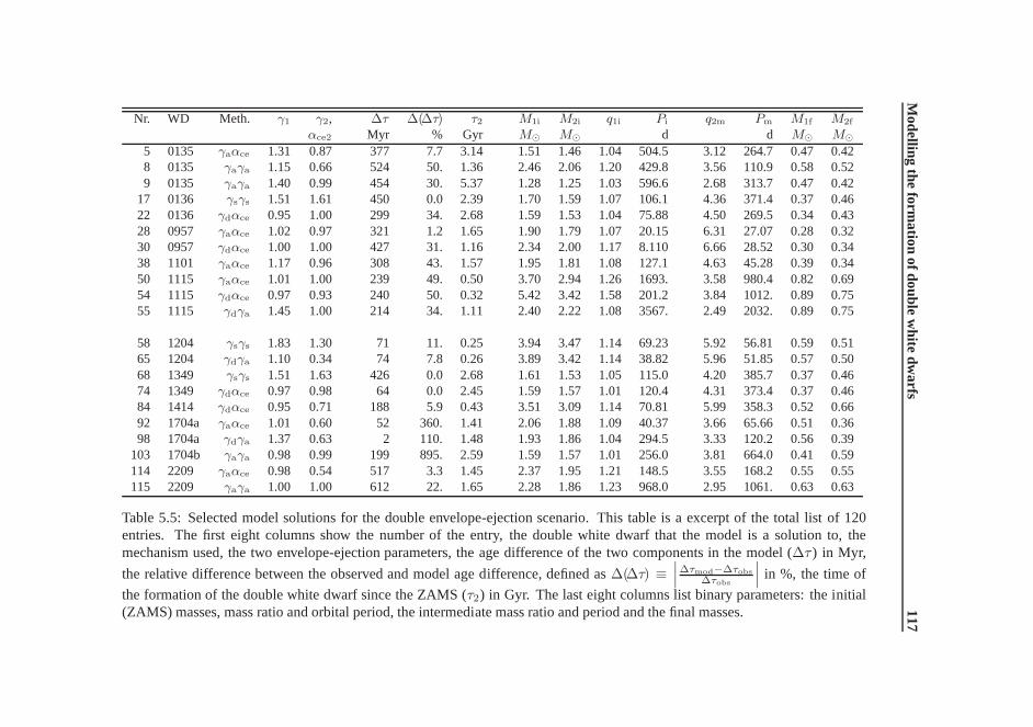
Modelling
theform
ationofdouble
white
dwarfs
117Nr. WD Meth. γ1 γ2, ∆τ ∆(∆τ) τ2 M1i M2i q1i Pi q2m Pm M1f M2f
αce2 Myr % Gyr M⊙ M⊙ d d M⊙ M⊙
5 0135 γaαce 1.31 0.87 377 7.7 3.14 1.51 1.46 1.04 504.5 3.12 264.7 0.47 0.428 0135 γaγa 1.15 0.66 524 50. 1.36 2.46 2.06 1.20 429.8 3.56 110.9 0.58 0.529 0135 γaγa 1.40 0.99 454 30. 5.37 1.28 1.25 1.03 596.6 2.68 313.7 0.47 0.42
17 0136 γsγs 1.51 1.61 450 0.0 2.39 1.70 1.59 1.07 106.1 4.36 371.4 0.37 0.4622 0136 γdαce 0.95 1.00 299 34. 2.68 1.59 1.53 1.04 75.88 4.50 269.5 0.34 0.4328 0957 γaαce 1.02 0.97 321 1.2 1.65 1.90 1.79 1.07 20.15 6.31 27.07 0.28 0.3230 0957 γdαce 1.00 1.00 427 31. 1.16 2.34 2.00 1.17 8.110 6.66 28.52 0.30 0.3438 1101 γaαce 1.17 0.96 308 43. 1.57 1.95 1.81 1.08 127.1 4.63 45.28 0.39 0.3450 1115 γaαce 1.01 1.00 239 49. 0.50 3.70 2.94 1.26 1693. 3.58 980.4 0.82 0.6954 1115 γdαce 0.97 0.93 240 50. 0.32 5.42 3.42 1.58 201.2 3.84 1012. 0.89 0.7555 1115 γdγa 1.45 1.00 214 34. 1.11 2.40 2.22 1.08 3567. 2.49 2032. 0.89 0.75
58 1204 γsγs 1.83 1.30 71 11. 0.25 3.94 3.47 1.14 69.23 5.92 56.81 0.59 0.5165 1204 γdγa 1.10 0.34 74 7.8 0.26 3.89 3.42 1.14 38.82 5.96 51.85 0.57 0.5068 1349 γsγs 1.51 1.63 426 0.0 2.68 1.61 1.53 1.05 115.0 4.20 385.7 0.37 0.4674 1349 γdαce 0.97 0.98 64 0.0 2.45 1.59 1.57 1.01 120.4 4.31 373.4 0.37 0.4684 1414 γdαce 0.95 0.71 188 5.9 0.43 3.51 3.09 1.14 70.81 5.99 358.3 0.52 0.6692 1704a γaαce 1.01 0.60 52 360. 1.41 2.06 1.88 1.09 40.37 3.66 65.66 0.51 0.3698 1704a γdγa 1.37 0.63 2 110. 1.48 1.93 1.86 1.04 294.5 3.33 120.2 0.56 0.39
103 1704b γaγa 0.98 0.99 199 895. 2.59 1.59 1.57 1.01 256.0 3.81 664.0 0.41 0.59114 2209 γaαce 0.98 0.54 517 3.3 1.45 2.37 1.95 1.21 148.5 3.55 168.2 0.55 0.55115 2209 γaγa 1.00 1.00 612 22. 1.65 2.28 1.86 1.23 968.0 2.95 1061. 0.63 0.63
Table 5.5: Selected model solutions for the double envelope-ejection scenario. This table is a excerpt of the total listof 120entries. The first eight columns show the number of the entry,the double white dwarf that the model is a solution to, themechanism used, the two envelope-ejection parameters, theage difference of the two components in the model (∆τ ) in Myr,
the relative difference between the observed and model age difference, defined as∆(∆τ) ≡∣
∣
∣
∆τmod−∆τobs
∆τobs
∣
∣
∣in %, the time of
the formation of the double white dwarf since the ZAMS (τ2) in Gyr. The last eight columns list binary parameters: the initial(ZAMS) masses, mass ratio and orbital period, the intermediate mass ratio and period and the final masses.
118 Chapter 5
acceptable age differences. The solutions 17 and 22 for WD 0136+768 and 28 and 30 forWD 0957–666 have values close to desired for both envelope-ejection parameters and the∆τ . Solution 38 is by far the best solution for WD 1101+364, thoughγa1 is not very closeto unity. Solutions 50 and 54 for PG 1115+116 have envelope-ejection parameters closeto the desired values and acceptable∆τ ’s, though the initial masses are high. This is inaccordance with the fact that these stars are required to form white dwarfs with masses ashigh as 0.7M⊙. Solution 55 shows that one has to accept a large value forγd1 in order tofind a solution with significantly smaller initial masses.
Solutions 58 and 65 are the only two for WD 1204+450 from the complete table thathave age differences within 50% of the observed value, and still the envelope-ejection pa-rameters are far from the desired values. There seems to be noconvincing solution for thissystem in our models. For WD 1349+144 the cooling ages are notknown, although thesimilar Balmer spectra of the two components (Karl et al. 2003a) seem to suggest that∆τis small. Solution 74 (which is the same as solutions 66, 69 and 70 in the complete table butwith a different definition ofγ) has a small age difference of 64 Myr but also a disturbinglysmall initial mass ratio of 1.01. Since the orbital period issupposed to increase with morethan 200% during the first dynamical mass-loss episode, it isuncertain how this initial sys-tem would evolve. Solution 68 has a larger initial mass ratio, but also a larger age difference.The complete table shows solutions for WD 1349+144 with values for∆τ of about 64, 140,230, 370 and 450 Myr, so that they span a large range within which the actual age differenceis likely to lie. For HE 1414–0848 we find an acceptable solution for almost all mechanismsand 4 out of the 8 solutions listed in the complete table referto the same solution withdifferent values for the envelope-ejection parameters forthe different mechanisms. Sincethe observed age difference of WD 1704+481a is−20Myr, we have introduced a systemwith the reversed mass ratio (WD 1704+481b) and hence an age difference of+20Myr.Interestingly enough, the solutions with closest age difference for WD 1704+481b have∆τ ∼>180Myr, a factor of nine or more than observed, as is the case for solution 103. How-ever, for WD 1704+481a we find solutions with good envelope-ejection parameters and anage difference of around 50 Myr, like solution 92, and with parameters that are more off, butwith an age difference of only 2 Myr as in solution 98. The system WD 1704+481a seemstherefore better explained by our models than the system with the reverse mass ratio. Be-cause the observed cooling-age difference is only in the order of a few per cent of the totalage of the system (see Table5.1), a change of 10% in the determined cooling age of one ofthe two components is sufficient to alter the age difference from−20 Myr to +50Myr. ForHE 2209–1444, we present solutions 114 and 115, that have envelope-ejection parametersclose to the desired values and an age difference that agreesvery well with the observedcooling-age difference.
Summarising, we find that for the ten observed systems, two can only be explainedwith values forγ that differ appreciably from the desired values (WD 0135–052 (31%) andWD 1204+450 (20%)). For two systems the values of the envelope-ejection parametersand age difference may not be too convincing, partially due to uncertainties in the observa-tions (WD 1101+364 (γ = 1.17) and WD 1704+481(a) (∆τ = 52 Myr)) and the other six
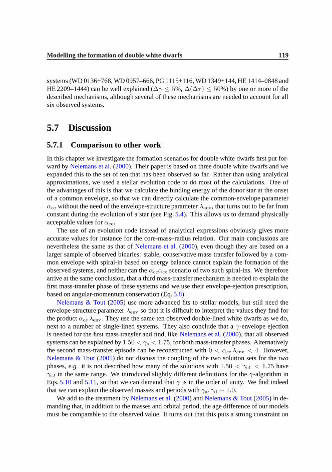
Modelling the formation of double white dwarfs 119
systems (WD 0136+768, WD 0957–666, PG 1115+116, WD 1349+144, HE 1414–0848 andHE 2209–1444) can be well explained (∆γ ≤ 5%, ∆(∆τ) ≤ 50%) by one or more of thedescribed mechanisms, although several of these mechanisms are needed to account for allsix observed systems.
5.7 Discussion
5.7.1 Comparison to other work
In this chapter we investigate the formation scenarios for double white dwarfs first put for-ward byNelemans et al.(2000). Their paper is based on three double white dwarfs and weexpanded this to the set of ten that has been observed so far. Rather than using analyticalapproximations, we used a stellar evolution code to do most of the calculations. One ofthe advantages of this is that we calculate the binding energy of the donor star at the onsetof a common envelope, so that we can directly calculate the common-envelope parameterαce without the need of the envelope-structure parameterλenv, that turns out to be far fromconstant during the evolution of a star (see Fig.5.4). This allows us to demand physicallyacceptable values forαce.
The use of an evolution code instead of analytical expressions obviously gives moreaccurate values for instance for the core-mass–radius relation. Our main conclusions arenevertheless the same as that ofNelemans et al.(2000), even though they are based on alarger sample of observed binaries: stable, conservative mass transfer followed by a com-mon envelope with spiral-in based on energy balance cannot explain the formation of theobserved systems, and neither can theαceαce scenario of two such spiral-ins. We thereforearrive at the same conclusion, that a third mass-transfer mechanism is needed to explain thefirst mass-transfer phase of these systems and we use their envelope-ejection prescription,based on angular-momentum conservation (Eq.5.8).
Nelemans & Tout(2005) use more advanced fits to stellar models, but still need theenvelope-structure parameterλenv so that it is difficult to interpret the values they find forthe productαce λenv. They use the same ten observed double-lined white dwarfs aswe do,next to a number of single-lined systems. They also concludethat aγ-envelope ejectionis needed for the first mass transfer and find, likeNelemans et al.(2000), that all observedsystems can be explained by1.50 < γs < 1.75, for both mass-transfer phases. Alternativelythe second mass-transfer episode can be reconstructed with0 < αce λenv < 4. However,Nelemans & Tout(2005) do not discuss the coupling of the two solution sets for the twophases,e.g. it is not described how many of the solutions with1.50 < γs1 < 1.75 haveγs2 in the same range. We introduced slightly different definitions for theγ-algorithm inEqs.5.10and5.11, so that we can demand thatγ is in the order of unity. We find indeedthat we can explain the observed masses and periods withγa, γd ∼ 1.0.
We add to the treatment byNelemans et al.(2000) andNelemans & Tout(2005) in de-manding that, in addition to the masses and orbital period, the age difference of our modelsmust be comparable to the observed value. It turns out that this puts a strong constraint on
120 Chapter 5
the selection of model solutions for all three definitions ofγ. However, we can still explainmost systems, although we need mass loss described by bothγa andγd to do so.
The description for dynamical mass loss with the specific angular momentum of thedonor star (Eq.5.11) is similar to the scenario of a tidally-enhanced stellar wind (Tout &Eggleton 1988b,a). In this scenario the mass loss from a (sub)giant due to stellar windincreases up to a factor of 150 with respect to Reimers’ empirical law (Reimers 1975) whenthe star is close to filling its Roche lobe.Tout & Eggleton(1988b) postulate the enhancedwind to explain for instance observed pre-Algol systems such as Z Her. In this binary themore evolved star is less massive than its main-sequence companion by 10%, while onlyfilling about half of its Roche lobe.
Han(1998) uses this tidally-enhanced stellar wind in his research onthe formation ofdouble degenerates and concludes, among others, that his models that include this enhancedstellar wind give a better explanation of the observed double-degenerate binaries than mod-els that do not include it. The enhanced mass loss makes subsequent mass transfer due toRoche-lobe overflow dynamically more stable. Envelope ejection due to dynamical massloss is then more often prevented and binaries evolve to longer orbital periods before thesecond mass transfer, which is then more likely to produce a CO white dwarf. Thus, theenhanced-wind scenario increases the ratio of CO-helium double white dwarfs to helium-helium binaries.
Envelope ejection described by Eq.5.11is essentially the same as the limiting case inwhich most or all of the envelope is lost due to an enhanced wind. Tout & Eggleton(1988b)show that the tidally-enhanced wind can indeed prevent Roche-lobe overflow altogetherbecause the envelope is completely lost by the wind and the core becomes exposed. Withoutan enhanced wind, this happens for binaries with an initial mass ratio of 2 or less only if theyhave initial periods of more than 1000 days. When the tidally-enhanced wind is included,core exposure without Roche-lobe overflow occurs for these binaries with initial periods asshort as 10–30days.
5.7.2 Alternative formation scenario for massive white dwarfs
In the present research we have assumed that after envelope ejection occurs, the core ofthe Roche-lobe filling giant becomes a helium or CO white dwarf with no further evolutionother than cooling. However, helium cores that are more massive than0.33 M⊙ are notdegenerate and those more massive than about0.5 M⊙ will burn most of the helium in theircores and produce a CO core. If exposed, they are in effect helium stars. For helium starsless massive than about0.75 M⊙ the radius hardly changes during the helium (shell) burn-ing, but stars more massive than that experience a giant phase. This is shown in Fig.5.16a,where the radius of a selection of helium-star models is plotted as a function of the CO-coremass. For the more massive models in the Figure, the stars expand from the order of a fewtenths of a solar radius to a few hundred solar radii. Thus, helium stars with a core massMCO ∼> 0.7 M⊙ may and those withMCO ∼> 0.8 M⊙ must become giants and could filltheir Roche lobes as a consequence. The black dots in Fig.5.16a indicate the maximum
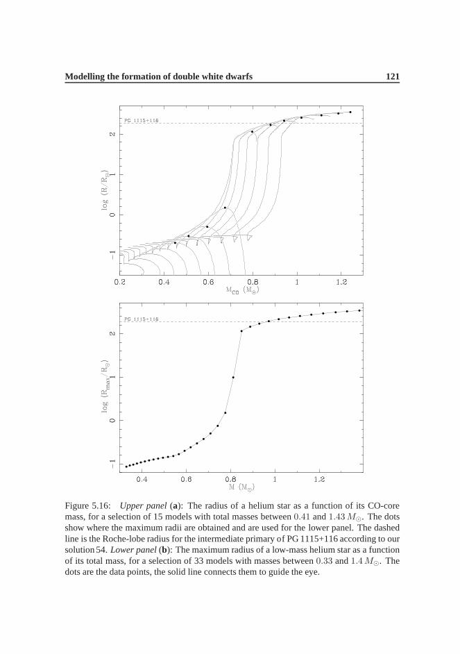
Modelling the formation of double white dwarfs 121
Figure 5.16: Upper panel(a): The radius of a helium star as a function of its CO-coremass, for a selection of 15 models with total masses between0.41 and1.43 M⊙. The dotsshow where the maximum radii are obtained and are used for thelower panel. The dashedline is the Roche-lobe radius for the intermediate primary of PG 1115+116 according to oursolution 54.Lower panel(b): The maximum radius of a low-mass helium star as a functionof its total mass, for a selection of 33 models with masses between0.33 and1.4 M⊙. Thedots are the data points, the solid line connects them to guide the eye.
122 Chapter 5
radius for a certain helium-star model and if we plot the maximum radii of these and othermodels as a function of the total mass of the star, we obtain Fig.5.16b. This Figure showsthat a helium star more massive than about0.83 M⊙ must evolve through a giant phase (seee.g. Paczynski 1971; Habets 1986).
There are two double white dwarfs in the observed sample thathaveM2 > 0.6 M⊙,PG 1115+116 (both components) and HE 1414–0848 (the secondary). The evolutionaryscenarios in Table5.5suggest that all these stars emerge from the envelope ejection with aCO core, except solution 54 for PG 1115+116, where the 5.42M⊙ primary progenitor pro-duces a 0.89M⊙ helium core before helium ignites. The Roche-lobe radius ofthe 0.89M⊙
helium star in the intermediate binary is 187R⊙ according to this solution and shown as thedashed line in Fig.5.16.
The Figure shows that the mass and Roche-lobe radius of this star are in the properrange to fit the helium-giant scenario. We show a small numerical example to illustrate thisscenario. The dot in Fig.5.16a atMCO=0.88M⊙ andR = 171 R⊙, just below the dashedline, is the point where the model of 0.93M⊙ from our grid of helium-star models reachesits largest radius. The star thus has an envelope mass of only0.05M⊙ and with a mass ratioof almost 4, mass transfer would be stable (Eq. 57 ofHurley et al.(2002)). If we assumethat this star would be the primary of solution 54 in Table5.5 and that 0.04M⊙ would betransferred conservatively, the orbital period after the mass transfer would be 1115d, so thatthe period would not change drastically and the ensuing second envelope ejection would besimilar to the one found in solution 54. If the mass were lost in a wind, which could betriggered by the fact that the star expands, but for which theRoche lobe need not be filled,the orbital period would change less than 2% to 1031 d. It seems that a complete, detailedmodel could be found to explain this system along these lines.
Both components in HE 1414–0848 are DA white dwarfs (Napiwotzki et al. 2002), asis the secondary of PG 1115+116. The hydrogen in the spectra of these stars suggests thatthe surface layer that formed after the envelope was ejectedis still present. However, theprimary in PG 1115+116 is a DB white dwarf. AsMaxted et al.(2002a) point out, the giantphase of a helium star could be the explanation for this and the scenario sketched abovemight indeed describe the formation of this system.
5.8 Conclusions
We investigated several formation scenarios for the observed ten double white dwarfs listedin Table5.1and present the best models in Table5.5. We draw four main conclusions:
• The scenario where the first mass-transfer phase is stable and conservative, followedby a common envelope with spiral-in based on energy conservation (see Eq.5.4) can-not explain the observed masses and periods of all double white dwarfs.
• The scenario with envelope ejection based on angular-momentum conservation fol-lowed by ejection of the second envelope with either energy or angular-momentumbalance can explain the observed masses and orbital periodsvery well.
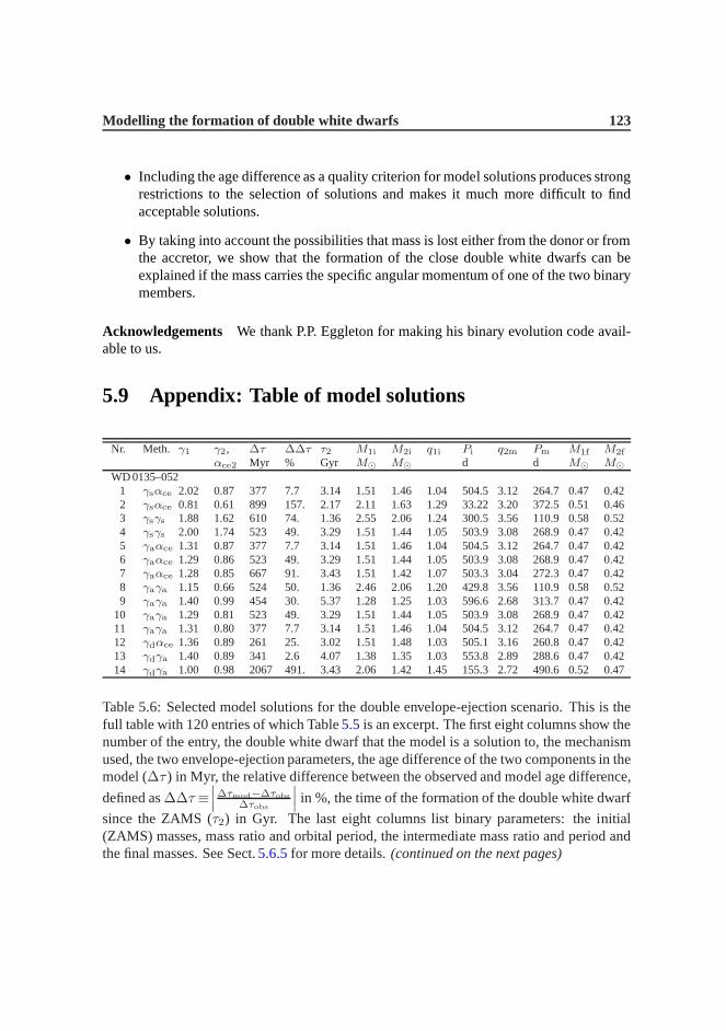
Modelling the formation of double white dwarfs 123
• Including the age difference as a quality criterion for model solutions produces strongrestrictions to the selection of solutions and makes it muchmore difficult to findacceptable solutions.
• By taking into account the possibilities that mass is lost either from the donor or fromthe accretor, we show that the formation of the close double white dwarfs can beexplained if the mass carries the specific angular momentum of one of the two binarymembers.
Acknowledgements We thank P.P. Eggleton for making his binary evolution code avail-able to us.
5.9 Appendix: Table of model solutions
Nr. Meth. γ1 γ2, ∆τ ∆∆τ τ2 M1i M2i q1i Pi q2m Pm M1f M2f
αce2 Myr % Gyr M⊙ M⊙ d d M⊙ M⊙
WD 0135–0521 γsαce 2.02 0.87 377 7.7 3.14 1.51 1.46 1.04 504.5 3.12 264.7 0.47 0.422 γsαce 0.81 0.61 899 157. 2.17 2.11 1.63 1.29 33.22 3.20 372.5 0.51 0.463 γsγs 1.88 1.62 610 74. 1.36 2.55 2.06 1.24 300.5 3.56 110.9 0.58 0.524 γsγs 2.00 1.74 523 49. 3.29 1.51 1.44 1.05 503.9 3.08 268.9 0.47 0.425 γaαce 1.31 0.87 377 7.7 3.14 1.51 1.46 1.04 504.5 3.12 264.7 0.47 0.426 γaαce 1.29 0.86 523 49. 3.29 1.51 1.44 1.05 503.9 3.08 268.9 0.47 0.427 γaαce 1.28 0.85 667 91. 3.43 1.51 1.42 1.07 503.3 3.04 272.3 0.47 0.428 γaγa 1.15 0.66 524 50. 1.36 2.46 2.06 1.20 429.8 3.56 110.9 0.58 0.529 γaγa 1.40 0.99 454 30. 5.37 1.28 1.25 1.03 596.6 2.68 313.7 0.47 0.42
10 γaγa 1.29 0.81 523 49. 3.29 1.51 1.44 1.05 503.9 3.08 268.9 0.47 0.4211 γaγa 1.31 0.80 377 7.7 3.14 1.51 1.46 1.04 504.5 3.12 264.7 0.47 0.4212 γdαce 1.36 0.89 261 25. 3.02 1.51 1.48 1.03 505.1 3.16 260.8 0.47 0.4213 γdγa 1.40 0.89 341 2.6 4.07 1.38 1.35 1.03 553.8 2.89 288.6 0.47 0.4214 γdγa 1.00 0.98 2067 491. 3.43 2.06 1.42 1.45 155.3 2.72 490.6 0.52 0.47
Table 5.6: Selected model solutions for the double envelope-ejection scenario. This is thefull table with 120 entries of which Table5.5is an excerpt. The first eight columns show thenumber of the entry, the double white dwarf that the model is asolution to, the mechanismused, the two envelope-ejection parameters, the age difference of the two components in themodel (∆τ ) in Myr, the relative difference between the observed and model age difference,
defined as∆∆τ ≡∣
∣
∣
∆τmod−∆τobs
∆τobs
∣
∣
∣in %, the time of the formation of the double white dwarf
since the ZAMS (τ2) in Gyr. The last eight columns list binary parameters: the initial(ZAMS) masses, mass ratio and orbital period, the intermediate mass ratio and period andthe final masses. See Sect.5.6.5for more details.(continued on the next pages)
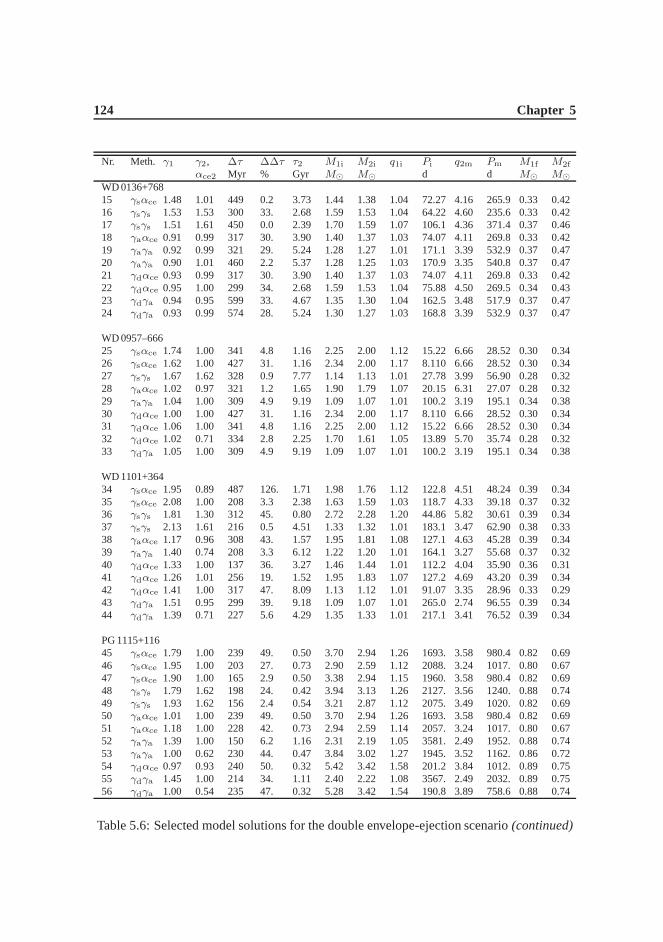
124 Chapter 5
Nr. Meth. γ1 γ2, ∆τ ∆∆τ τ2 M1i M2i q1i Pi q2m Pm M1f M2f
αce2 Myr % Gyr M⊙ M⊙ d d M⊙ M⊙
WD 0136+76815 γsαce 1.48 1.01 449 0.2 3.73 1.44 1.38 1.04 72.27 4.16 265.9 0.33 0.4216 γsγs 1.53 1.53 300 33. 2.68 1.59 1.53 1.04 64.22 4.60 235.6 0.33 0.4217 γsγs 1.51 1.61 450 0.0 2.39 1.70 1.59 1.07 106.1 4.36 371.4 0.37 0.4618 γaαce 0.91 0.99 317 30. 3.90 1.40 1.37 1.03 74.07 4.11 269.8 0.33 0.4219 γaγa 0.92 0.99 321 29. 5.24 1.28 1.27 1.01 171.1 3.39 532.9 0.37 0.4720 γaγa 0.90 1.01 460 2.2 5.37 1.28 1.25 1.03 170.9 3.35 540.8 0.37 0.4721 γdαce 0.93 0.99 317 30. 3.90 1.40 1.37 1.03 74.07 4.11 269.8 0.33 0.4222 γdαce 0.95 1.00 299 34. 2.68 1.59 1.53 1.04 75.88 4.50 269.5 0.34 0.4323 γdγa 0.94 0.95 599 33. 4.67 1.35 1.30 1.04 162.5 3.48 517.9 0.37 0.4724 γdγa 0.93 0.99 574 28. 5.24 1.30 1.27 1.03 168.8 3.39 532.9 0.37 0.47
WD 0957–66625 γsαce 1.74 1.00 341 4.8 1.16 2.25 2.00 1.12 15.22 6.66 28.52 0.30 0.3426 γsαce 1.62 1.00 427 31. 1.16 2.34 2.00 1.17 8.110 6.66 28.52 0.30 0.3427 γsγs 1.67 1.62 328 0.9 7.77 1.14 1.13 1.01 27.78 3.99 56.90 0.28 0.3228 γaαce 1.02 0.97 321 1.2 1.65 1.90 1.79 1.07 20.15 6.31 27.07 0.28 0.3229 γaγa 1.04 1.00 309 4.9 9.19 1.09 1.07 1.01 100.2 3.19 195.1 0.34 0.3830 γdαce 1.00 1.00 427 31. 1.16 2.34 2.00 1.17 8.110 6.66 28.52 0.30 0.3431 γdαce 1.06 1.00 341 4.8 1.16 2.25 2.00 1.12 15.22 6.66 28.52 0.30 0.3432 γdαce 1.02 0.71 334 2.8 2.25 1.70 1.61 1.05 13.89 5.70 35.74 0.28 0.3233 γdγa 1.05 1.00 309 4.9 9.19 1.09 1.07 1.01 100.2 3.19 195.1 0.34 0.38
WD 1101+36434 γsαce 1.95 0.89 487 126. 1.71 1.98 1.76 1.12 122.8 4.51 48.24 0.39 0.3435 γsαce 2.08 1.00 208 3.3 2.38 1.63 1.59 1.03 118.7 4.33 39.18 0.37 0.3236 γsγs 1.81 1.30 312 45. 0.80 2.72 2.28 1.20 44.86 5.82 30.61 0.39 0.3437 γsγs 2.13 1.61 216 0.5 4.51 1.33 1.32 1.01 183.1 3.47 62.90 0.38 0.3338 γaαce 1.17 0.96 308 43. 1.57 1.95 1.81 1.08 127.1 4.63 45.28 0.39 0.3439 γaγa 1.40 0.74 208 3.3 6.12 1.22 1.20 1.01 164.1 3.27 55.68 0.37 0.3240 γdαce 1.33 1.00 137 36. 3.27 1.46 1.44 1.01 112.2 4.04 35.90 0.36 0.3141 γdαce 1.26 1.01 256 19. 1.52 1.95 1.83 1.07 127.2 4.69 43.20 0.39 0.3442 γdαce 1.41 1.00 317 47. 8.09 1.13 1.12 1.01 91.07 3.35 28.96 0.33 0.2943 γdγa 1.51 0.95 299 39. 9.18 1.09 1.07 1.01 265.0 2.74 96.55 0.39 0.3444 γdγa 1.39 0.71 227 5.6 4.29 1.35 1.33 1.01 217.1 3.41 76.52 0.39 0.34
PG 1115+11645 γsαce 1.79 1.00 239 49. 0.50 3.70 2.94 1.26 1693. 3.58 980.4 0.82 0.6946 γsαce 1.95 1.00 203 27. 0.73 2.90 2.59 1.12 2088. 3.24 1017. 0.80 0.6747 γsαce 1.90 1.00 165 2.9 0.50 3.38 2.94 1.15 1960. 3.58 980.4 0.82 0.6948 γsγs 1.79 1.62 198 24. 0.42 3.94 3.13 1.26 2127. 3.56 1240. 0.88 0.7449 γsγs 1.93 1.62 156 2.4 0.54 3.21 2.87 1.12 2075. 3.49 1020. 0.82 0.6950 γaαce 1.01 1.00 239 49. 0.50 3.70 2.94 1.26 1693. 3.58 980.4 0.82 0.6951 γaαce 1.18 1.00 228 42. 0.73 2.94 2.59 1.14 2057. 3.24 1017. 0.80 0.6752 γaγa 1.39 1.00 150 6.2 1.16 2.31 2.19 1.05 3581. 2.49 1952. 0.88 0.7453 γaγa 1.00 0.62 230 44. 0.47 3.84 3.02 1.27 1945. 3.52 1162. 0.86 0.7254 γdαce 0.97 0.93 240 50. 0.32 5.42 3.42 1.58 201.2 3.84 1012. 0.89 0.7555 γdγa 1.45 1.00 214 34. 1.11 2.40 2.22 1.08 3567. 2.49 2032. 0.89 0.7556 γdγa 1.00 0.54 235 47. 0.32 5.28 3.42 1.54 190.8 3.89 758.6 0.88 0.74
Table 5.6: Selected model solutions for the double envelope-ejection scenario(continued)
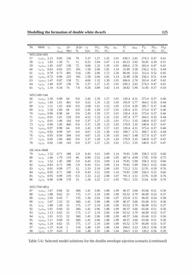
Modelling the formation of double white dwarfs 125
Nr. Meth. γ1 γ2, ∆τ ∆∆τ τ2 M1i M2i q1i Pi q2m Pm M1f M2f
αce2 Myr % Gyr M⊙ M⊙ d d M⊙ M⊙
WD 1204+45057 γsαce 2.15 0.83 136 70. 5.37 1.27 1.25 1.01 630.3 2.65 274.3 0.47 0.4158 γsγs 1.83 1.30 71 11. 0.25 3.94 3.47 1.14 69.23 5.92 56.81 0.59 0.5159 γaαce 1.45 0.87 138 72. 4.66 1.32 1.30 1.01 606.6 2.76 263.4 0.47 0.4160 γaγa 0.63 0.65 225 181. 1.58 2.06 1.81 1.14 32.89 3.58 256.2 0.51 0.4461 γaγa 0.78 0.72 491 514. 1.85 2.06 1.72 1.20 86.06 3.33 312.4 0.52 0.4562 γdαce 0.72 0.96 225 181. 1.58 2.06 1.81 1.14 32.89 3.58 256.2 0.51 0.4463 γdαce 1.47 0.87 138 72. 4.66 1.32 1.30 1.01 606.6 2.76 263.4 0.47 0.4164 γdγa 1.49 0.97 136 70. 5.37 1.27 1.25 1.01 630.3 2.65 274.3 0.47 0.4165 γdγa 1.10 0.34 74 7.8 0.26 3.89 3.42 1.14 38.82 5.96 51.85 0.57 0.50
WD 1349+14466 γsαce 1.56 0.98 64 0.0 2.45 1.59 1.57 1.01 120.4 4.31 373.4 0.37 0.4667 γsαce 1.45 1.01 461 0.0 4.52 1.35 1.32 1.03 105.9 3.77 364.5 0.35 0.4468 γsγs 1.51 1.63 426 0.0 2.68 1.61 1.53 1.05 115.0 4.20 385.7 0.37 0.4669 γsγs 1.56 1.60 64 0.0 2.45 1.59 1.57 1.01 120.4 4.31 373.4 0.37 0.4670 γaαce 0.96 0.98 64 0.0 2.45 1.59 1.57 1.01 120.4 4.31 373.4 0.37 0.4671 γaαce 0.91 1.01 229 0.0 4.52 1.33 1.32 1.01 107.4 3.77 364.5 0.35 0.4472 γaγa 0.91 1.00 143 0.0 5.37 1.27 1.25 1.01 173.1 3.35 540.8 0.37 0.4773 γaγa 0.90 1.00 460 0.0 5.37 1.28 1.25 1.03 170.9 3.35 540.8 0.37 0.4774 γdαce 0.97 0.98 64 0.0 2.45 1.59 1.57 1.01 120.4 4.31 373.4 0.37 0.4675 γdαce 0.92 0.99 147 0.0 4.67 1.32 1.30 1.01 108.7 3.72 369.7 0.35 0.4476 γdγa 0.93 0.94 368 0.0 4.67 1.33 1.30 1.03 164.7 3.48 517.9 0.37 0.4777 γdγa 0.92 1.00 460 0.0 5.37 1.28 1.25 1.03 170.9 3.35 540.8 0.37 0.4778 γdγa 0.92 1.00 143 0.0 5.37 1.27 1.25 1.01 173.1 3.35 540.8 0.37 0.47
HE 1414–084879 γsαce 1.52 0.71 188 5.9 0.43 3.51 3.09 1.14 70.81 5.99 358.3 0.52 0.6680 γsγs 1.46 1.79 119 40. 0.90 2.52 2.40 1.05 467.4 4.09 1720. 0.59 0.7581 γsγs 1.52 1.45 188 5.9 0.43 3.51 3.09 1.14 70.81 5.99 358.3 0.52 0.6682 γaαce 0.83 0.71 188 5.9 0.43 3.51 3.09 1.14 70.81 5.99 358.3 0.52 0.6683 γaγa 0.91 0.99 177 12. 1.33 2.19 2.08 1.05 712.2 3.51 2170. 0.59 0.7684 γdαce 0.95 0.71 188 5.9 0.43 3.51 3.09 1.14 70.81 5.99 358.3 0.52 0.6685 γdγa 0.95 0.99 219 9.5 1.33 2.22 2.08 1.07 701.3 3.51 2170. 0.59 0.7686 γdγa 0.96 0.98 170 15. 1.28 2.22 2.11 1.05 702.1 3.55 2134. 0.59 0.76
WD 1704+481a87 γsαce 1.67 0.60 52 360. 1.41 2.06 1.88 1.09 40.37 3.66 65.66 0.51 0.3688 γsαce 1.88 0.62 15 175. 1.17 2.19 2.00 1.09 93.52 3.79 66.89 0.53 0.3789 γsαce 2.05 0.43 7 135. 1.36 2.03 1.90 1.07 252.8 3.51 96.02 0.54 0.3890 γsγs 1.67 1.52 52 360. 1.41 2.06 1.88 1.09 40.37 3.66 65.66 0.51 0.3691 γsγs 1.88 1.50 15 175. 1.17 2.19 2.00 1.09 93.52 3.79 66.89 0.53 0.3792 γaαce 1.01 0.60 52 360. 1.41 2.06 1.88 1.09 40.37 3.66 65.66 0.51 0.3693 γaαce 1.13 0.62 15 175. 1.17 2.19 2.00 1.09 93.52 3.79 66.89 0.53 0.3794 γaγa 1.01 0.55 52 360. 1.41 2.06 1.88 1.09 40.37 3.66 65.66 0.51 0.3695 γdαce 1.11 0.60 52 360. 1.41 2.06 1.88 1.09 40.37 3.66 65.66 0.51 0.3696 γdαce 1.24 0.62 15 175. 1.17 2.19 2.00 1.09 93.52 3.79 66.89 0.53 0.3797 γdαce 1.37 0.34 2 110. 1.48 1.93 1.86 1.04 294.5 3.33 120.2 0.56 0.3998 γdγa 1.37 0.63 2 110. 1.48 1.93 1.86 1.04 294.5 3.33 120.2 0.56 0.39
Table 5.6: Selected model solutions for the double envelope-ejection scenario(continued)

126 Chapter 5
Nr. Meth. γ1 γ2, ∆τ ∆∆τ τ2 M1i M2i q1i Pi q2m Pm M1f M2f
αce2 Myr % Gyr M⊙ M⊙ d d M⊙ M⊙
WD 1704+481b99 γsαce 1.65 0.53 292 1360. 0.73 2.83 2.59 1.09 47.21 6.37 161.8 0.41 0.58100 γsαce 1.74 0.76 285 1326. 0.75 2.76 2.55 1.08 49.12 6.40 107.3 0.40 0.57101 γsγs 1.64 1.87 182 810. 2.23 1.68 1.65 1.01 212.1 4.08 478.6 0.41 0.58102 γaαce 0.96 1.05 465 2223. 1.00 2.62 2.31 1.14 44.02 6.10 63.28 0.38 0.54103 γaγa 0.98 0.99 199 895. 2.59 1.59 1.57 1.01 256.0 3.81 664.0 0.41 0.59104 γaγa 0.94 0.97 181 805. 2.23 1.68 1.65 1.01 284.0 3.88 892.6 0.43 0.61105 γdαce 1.03 0.15 182 810. 2.23 1.68 1.65 1.01 212.1 4.08 478.6 0.41 0.58106 γdαce 1.00 0.76 332 1562. 0.75 2.87 2.55 1.12 33.29 6.40 107.3 0.40 0.57107 γdγa 0.95 0.97 181 805. 2.23 1.68 1.65 1.01 284.0 3.88 892.6 0.43 0.61108 γdγa 1.00 0.99 199 895. 2.59 1.59 1.57 1.01 256.0 3.81 664.0 0.41 0.59
HE 2209–1444109 γsαce 1.69 0.54 517 3.3 1.45 2.37 1.95 1.21 148.5 3.55 168.2 0.55 0.55110 γsαce 1.56 0.88 552 10. 0.75 3.79 2.55 1.49 87.01 4.48 113.8 0.57 0.57111 γsγs 1.62 1.64 262 48. 1.20 2.37 2.16 1.09 150.0 3.93 304.6 0.55 0.55112 γsγs 1.63 1.73 510 2.1 1.24 2.59 2.14 1.21 403.6 3.62 596.1 0.59 0.59113 γaαce 1.19 0.90 42 92. 1.20 2.19 2.16 1.01 121.7 4.08 97.10 0.53 0.53114 γaαce 0.98 0.54 517 3.3 1.45 2.37 1.95 1.21 148.5 3.55 168.2 0.55 0.55115 γaγa 1.00 1.00 612 22. 1.65 2.28 1.86 1.23 968.0 2.95 1061. 0.63 0.63116 γaγa 1.08 1.00 499 0.2 1.87 2.06 1.76 1.17 809.5 2.94 777.6 0.60 0.60117 γdαce 1.06 0.53 347 31. 1.35 2.31 2.03 1.14 80.61 3.76 169.5 0.54 0.54118 γdαce 1.12 0.88 559 12. 0.75 3.84 2.55 1.50 71.51 4.48 113.8 0.57 0.57119 γdγa 1.15 0.86 744 49. 1.35 2.76 2.03 1.36 556.8 3.27 881.7 0.62 0.62120 γdγa 1.00 0.81 731 46. 1.48 2.55 1.93 1.32 135.6 3.38 437.5 0.57 0.57
Table 5.6: Selected model solutions for the double envelope-ejection scenario(continued)


![ON MODELLING OF MICROSTRUCTURE FORMATION, LOCAL …2]_JH.pdf1(8) ON MODELLING OF MICROSTRUCTURE FORMATION, LOCAL MECHANICAL PROPERTIES AND STRESS – STRAIN DEVELOPMENT IN ALUMINIUM](https://img.pdfslide.net/doc/110x75/5e4a839e60f849345a4bd5ca/on-modelling-of-microstructure-formation-local-2jhpdf-18-on-modelling-of-microstructure.jpg)